
Submitted:
14 January 2026
Posted:
15 January 2026
You are already at the latest version
Abstract
The robotic arm of the Wentian module can complete tasks such as supporting astronauts' extravehicular activities, installing and maintaining payloads, and inspecting the space station. The 7-joint SSRMS manipulator is critical for space missions. This study aims to build its kinematic model via screw theory. It simplifies SSRMS to right-angle rods, defines joint screw axes, twist coordinates, and initial pose matrix. Using PoE formula, the 7-DOF forward kinematics equation is derived. Besides, it derives fixed joint angle for inverse kinematics, including analytical solutions and numerical solutions. It elaborates analytical solutions for fixing joints 1/7 and 2/6 and numerical solutions for fixing joints 3/4/5,solves all joint angles via kinematic decoupling, and addresses special cases. Experiments with China’s space station small arm parameters show The probability of meeting the accuracy threshold of 10−4 is 99.79%,verifying model effectiveness, while noting singularity-related weak solving areas. This provides a reliable basis for subsequent inverse kinematics optimization.
Keywords:
SSRMS manipulator
; screw theory
; kinematic modeling
; fixed joint angle method
; analytical solution
; numerical solutions
; inverse kinematics
1. Introduction
The full completion and stable operation of China's space station marks a new stage of "space station application and development" for China's manned space program. As a core scientific research platform in low Earth orbit, its 400-450km orbit deployment, 10-year design life and three-module T-shaped configuration enable the long-term stay of three astronauts, highlighting the leap of China's aerospace industry from "following" to "taking the lead", and laying the foundation for deep space exploration [1].
The space station's robotic arm system adopts a "dual-arm coordination" architecture, consisting of the core module and the robotic arm of the Wentian module [1]. The core module's robotic arm focuses on heavy-load tasks, while the Wentian module's robotic arm has a higher end positioning accuracy. It is responsible for assisting astronauts during extravehicular activities,conducting meticulous maintenance of payloads, and inspecting equipment. Its performance directly affects the operational efficiency of the space station [1,2].
Inverse kinematics is the foundation of path planning and reachability analysis for robotic arms [3]. The mechanical arm of the Wentian module is a 7-degree-of-freedom redundant mechanical arm in the SSRMS configuration (with 3 rotating joints each for the shoulder and wrist and 1 for the elbow) [1]. The redundant degrees of freedom enhance operational flexibility, but the shoulder and wrist offset and redundancy characteristics lead to multiple solutions in inverse kinematics, increasing the difficulty of solving [4,5,6]. Scholars pointed out that the offset pose of the SSRMS configuration would intensify the instability of the solutions provided by traditional methods [5].
Scholars at home and abroad have conducted research on the inverse solution of SSRMS: Pieper proposed a 6-degree-of-freedom closed inverse solution criterion [7]; Siciliano classified the methods into geometric analytical methods and numerical iterative methods. Zhao Zhiyuan et al. in China proposed the DH parameter method model [8], and the team from Journal of Mechanical Engineering proposed the CCDJAP-IK method to improve the accuracy of the solution [9]. International Faria et al. proposed the position-based method [10], Ma Boyu et al. proposed the optimization idea of minimizing speed-acceleration for obstacle avoidance [11], and Luo Shuangbao et al. proposed the differential evolution algorithm [12].
The existing methods have shortcomings: the DH parameter method is difficult to characterize the shoulder and wrist offset [8]; The convergence of near-singularities in numerical methods is unstable [1]; The analytical method has poor universality [7]; The offset pose problem has not been fully solved [5].The traditional inverse kinematics control strategy of the kinematic model of redundant robotic arms has shortcomings such as the lack of intuitive workspace modeling[13],non-unique inverse solutions[14], high computational overhead[15], limited adaptability to special configurations and complex working scenarios[16], and is prone to insufficient solution stability in singular regions.For this popose,improved inverse kinematics analysis involves substituting the joint angles obtained based on the spiral theory and inverse kinematics solution into the forward kinematics model of the robotic arm to determine the pose of the end effector at the current moment[17].It can achieve smooth[18] and stable[19] control of the mechanical arm.Based on the spiral theory modeling, combined with the parameter optimization idea of the CCDJAP-IK method and the optimization strategy[5,9,11], through the fixed joint Angle method and decoupling solution, the accuracy and stability of the inverse solution are improved [20,21], and the experimental verification accuracy rate reaches 99.79%.
2. Forward Kinematics
2.1. Mechanical Arm Model
The forward kinematics model of the robotic arm as shown in the following figure was established by using the spinor method.
Figure 1.
Spinometric model.
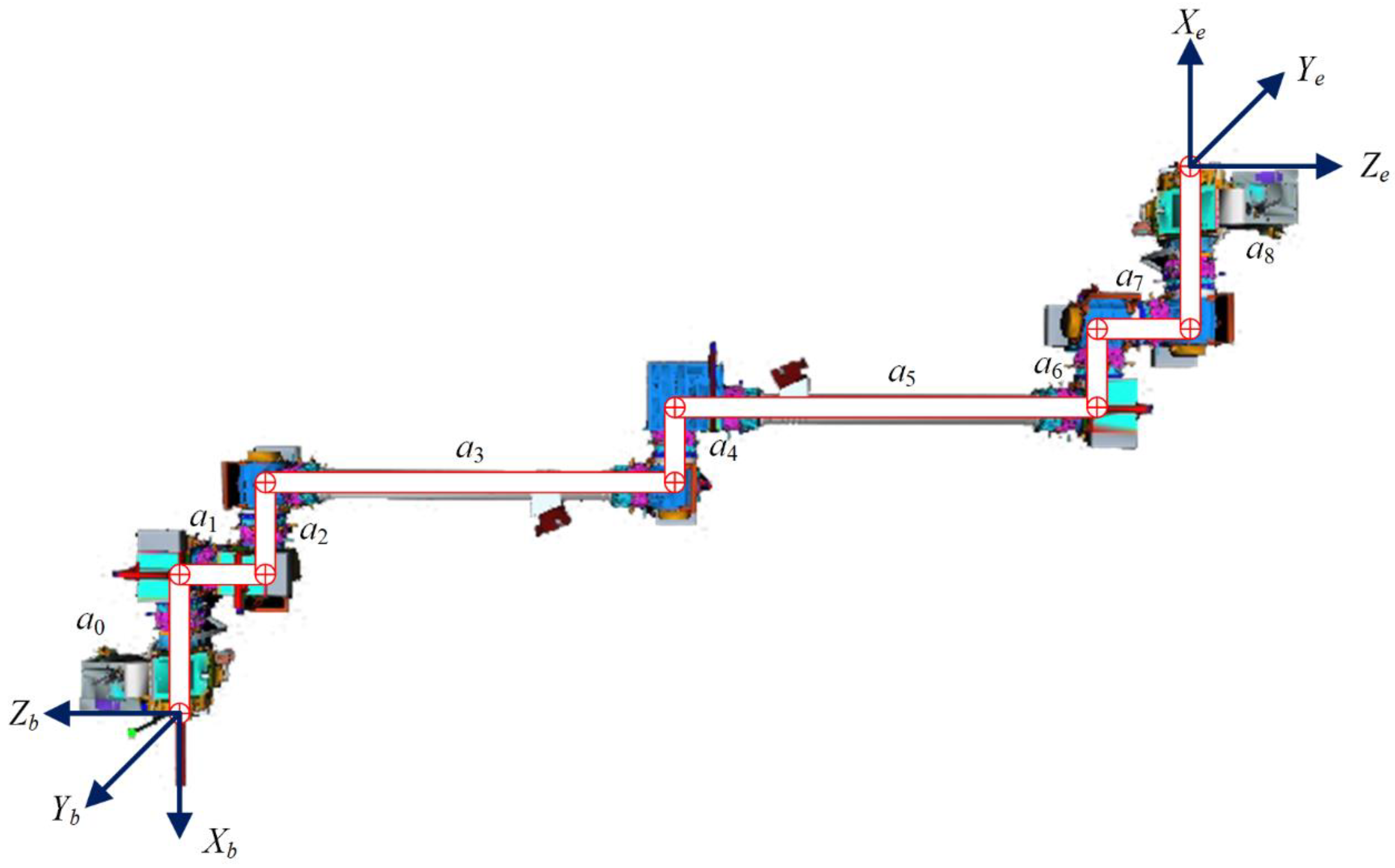

Table 1.
Member Parameters (mm).
| 716.1 | 430 | 430 | 2080 | 387 | 2080 | 430 | 430 | 716.1 |
The corresponding member parameter information is as follows:
In the initial state, the pose matrix of the terminal system relative to the base coordinate system is as follows:
2.2. Definition of the Spiral Shaft
Taking the base coordinate system as the reference coordinate system, the helical axes of each joint are described as follows, where represents the representation of the unit vector along the positive direction of the joint axis in the reference coordinate system; represents the measurement of the coordinate values of any point on the joint axis in the reference coordinate.
The spinor coordinates corresponding to the helical axis are shown in the following table. Note that represents the angular velocity of the object coordinate system relative to the reference coordinate system;represents the instantaneous linear velocity at the point where the rigid body coincides with the origin of the reference coordinate system, rather than the absolute linear velocity at the origin of the object's coordinate system.
2.3. Forward Kinematics Equations
The corresponding Lie algebraic form of each spiral axis motion screw is given below:
Note: [] is the cross-product matrix corresponding to.
The calculation of the matrix exponential of is as follows:
According to the PoE(Product of Exponentials) formula, the forward kinematics expression for the SSRMS configuration 7-DOF robotic arm is derived as follows:
3. Inverse Kinematics
3.1. Pieper Criteria
When one of the following conditions is met, a 6-degree-of-freedom kinematic structure has a closed kinematic inverse solution:
- The axes of three consecutive rotating joints intersect at the same point.
- three consecutive parallel to the axis of the rotation of the joint.[10]
Meanwhile, during the process of solving inverse kinematics, the following three fundamental principles need to be followed:
- Position invariance: For pure rotational motion spirals, the position of any point P on the axis remains unchanged.
- Constant distance: For the scalar of pure rotational motion, the distance from any point P not on the rotating shaft to the fixed point R on the rotating shaft remains constant.
- Invariant attitude: For pure moving motion spirals, the attitude of any point P in space remains unchanged before and after the transformation.[21]
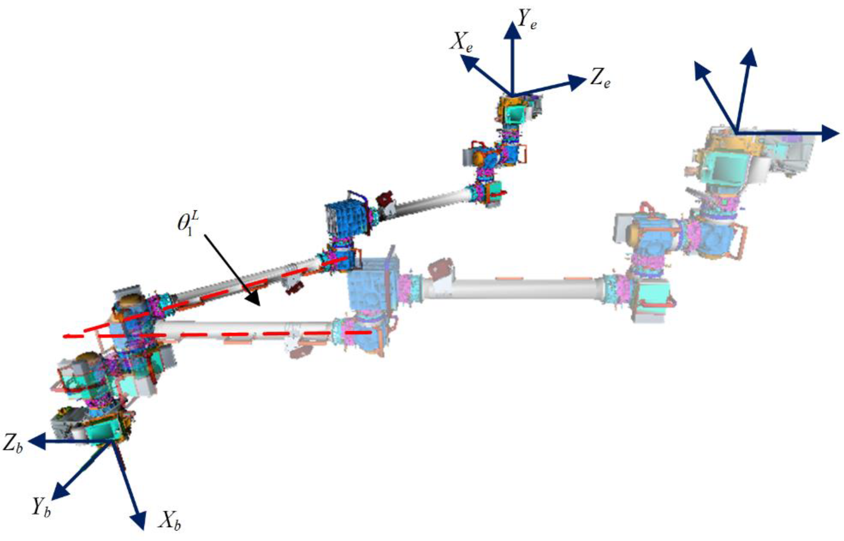
For the SSRMS configuration robotic arm, the axes of the three consecutive joints, namely joint 3, joint 4, and joint 5, are parallel. Assuming that one of the joints, namely joint 1, joint 2, joint 6, and joint 7, has a fixed Angle, there exists an analytical solution for the remaining six joints. Considering the symmetrical characteristics of the robotic arm configuration design, it is only necessary to study the analytical solution methods under the conditions of fixed joint 1 or fixed joint 2, as well as the numerical solution methods under the conditions of fixed joint 3 or fixed joint 4.
3.2. Analytical Solution of the Fixed Joint Angle Method
3.2.1. Fix the Joint 1/7
Considering the symmetry of the SSMRS configuration manipulator, the solution methods for fixing angle 1 and fixing angle 7 are consistent. Here, only the position-level inverse solution algorithm for fixing joint 1 is discussed.
Assuming the angle of joint 1 is , the transformation process is as follows:
Figure 2.
The Transformation of Joint 1 Angle.
With the base coordinate system as the reference coordinate system, the initial pose matrix of the equivalent 6-DOF manipulator can be expressed as:
Based on the principle of coordinate transformation for motion screws, the motion screw corresponding to the new screw axis is as follows:
Further derive the forward kinematics equations for the equivalent 6-DOF manipulator:
Reorganizing the known terms, we have:
Assuming the intersection point of joint 6 and joint 7 is represented as Pa in the base coordinate system, according to the principle of position invariance, we have:
Based on the definition of the zero-position coordinate system, it can be concluded that:
Substituting into equation(9), can obtain:
The above equation can be interpreted as the spatial point first rotating around by to point, then rotating around by to point , next rotating around by to point , and finally rotating around by to point , as shown in Figure 3:
Let the transformed coordinates of be , then we have:
It can be observed that both before transformation and after transformation are known quantities.
Based on the geometric relationships in the figure and the principle of distance invariance, it can be concluded that:
where, is the intersection point of the axes of joint 1 and joint 2.
According to equation(7), we can obtain:
Assuming , based on equation (14-1), we can obtain:
The specific physical meaning is shown in Figure 4. Point lies on a sphere with center at and on the plane , with their intersection forming a spatial circle. Additionally, point lies within a sectional plane related to , represented in point-normal form as a plane passing through with a normal vector .
Further analyzing the cutting plane , it can be concluded that point has two solutions, and , corresponding to the results of rotating and around the spiral axis of joint 1, as shown in Figure 5.
Let:
Conditions for the existence of solutions:
Then the solution is as follows:
Further derived solutions for are as follows:
On this basis, consider the following constraint relationships:
Based on Paden-Kahan Subproblem 1, the angle of joint 2 can be determined. The forward kinematics equations can be further simplified into:
Regarding the above equation, further solution will be provided in Section 3.2.3.
3.2.2. Fix the Joint 2/6
Considering the symmetry of the SSMRS configuration manipulator, the solution methods for fixing angle 2 and fixing angle 6 are consistent. Here, only the position-level inverse solution algorithm for fixing joint 2 is discussed.
Assuming the angle of joint 2 is , the transformation process is shown in Figure 6:
With the base coordinate system as the reference, the initial pose matrix of the equivalent 6-DOF manipulator can be expressed as:
Based on the principle of coordinate transformation for motion screws, the motion screw corresponding to the new screw axis is as follows:
Further derive the forward kinematics equations for the equivalent 6-DOF manipulator:
Reorganizing the known terms, we have:
Assuming the intersection point of joint 6 and joint 7 is represented as Pa in the base coordinate system, according to the principle of position invariance, we have::
Based on the definition of the zero-position coordinate system, it can be concluded that:
Substituting into Equation (28), can obtain:
The above equation can be interpreted as the spatial point first rotating around by to point , then rotating around by to point , next rotating around by to point , and finally rotating around by to point , as shown in Figure 7:
Let the transformed coordinates of be , then we have:
It can be observed that both before transformation and after transformation are known quantities.
Based on the geometric relationships in the figure and the principle of distance invariance, it can be concluded that:
where, is the origin of the base coordinate system, and is the intersection point of the axes of joint 1 and joint 2.
According to equation (27):
Assuming , based on equations (34-1) and (34-2), we can derive:
Substituting equation (36) into equation (34-3), we can obtain:
Let:
Conditions for the existence of solutions:
Then the solution is as follows:
Further derived solutions for are as follows:
On this basis, consider the following constraint relationships:
Based on Paden-Kahan Subproblem 1, the angle of joint 1 can be determined. The forward kinematics equations can be further simplified into:
Regarding the above equation, further solution will be provided in Section 3.2.3.
3.2.3. Kinematic Decoupling
Considering the following transformation relationships:
Constraints in the form of the following equation can be rewritten as follows:
Substituting into the equation to be solved, we can obtain:
Further, let:
Considering that joints 3, 4, and 5 are all rotations around the X-axis, the following constraints are analyzed:
Then, we can obtain:
Note that in the solution formulas for and , cannot be casually canceled out because its sign affects the quadrant position of the corresponding angle. Instead of dividing by , it can be changed to multiplying by . Additionally, the impact of a zero denominator should be considered. When is zero, depending on the value of , we have:
For simplicity, we can let = 0.
Once the values of and are obtained, substituting them into equation (48)and simplifying yields:
Analyze the following constraints:
Simplifying, we obtain:
Squaring and summing, we obtain:
With θ4 determined, equatio (54) can be further simplified into:
Solving equation (56) yields:
Further, we obtain:
Accordingly, all joint angle parameters can be determined. However, it is important to consider the joint limits when calculating the complete set of solutions for all joints.Avoid joint over-limit, and at the same time, all inverse solutions can be solved through .
3.3. Numerical Solution Method for Inverse Kinematics
3.3.1. Newton's Iterative Method
Newton's method, also known as the Newton-Raphson method, is a technique proposed by Newton in the 17th century for approximately solving equations in both the real number field and the complex number field. Most equations do not have a root formula, making it extremely difficult or even impossible to calculate an exact solution. Therefore, finding the approximate roots of an equation is particularly important. This method uses the first few terms of the Taylor series of the function to find the roots of the equation, and it is one of the important methods for finding the roots of equations. Its greatest advantage is that it has square convergence near the single root of the equation.[22]
3.3.2. Jacobian Matrix
For any joint configuration θ, the terminal velocity vector and the joint velocity vectorare linearly correlated. The mapping relationship between the two can be established through the Jacobian matrix, that is:
The end velocity is closely related to the generalized coordinates of the end, and conversely, it also affects the form of the Jacobian matrix. In most cases,is a six-dimensional motion spinor. The i-th column of the Jacobian matrix represents the rotational vector when and the velocities of all other joints are zero.[23]
Consider an N-bar open-chain robot. The formula for the exponential product of its forward kinematics is:
The spatial velocity can be written as , where
Furthermore
From this, we can obtain:
It is rewritten in vector form through adjoint mapping as follows:
Rewrite it as the vector sum of n spatial velocities:
It is written in matrix form as follows:
A matrix is a Jacobian matrix in the form of fixed spatial coordinates, abbreviated as spatial Jacobian. Observe the structural form of the i-th column as follows: where represents the spinor coordinates of the i-th joint relative to the fixed coordinate system when the robot is at zero position. Therefore, represents the spinor coordinates of the i-th joint relative to the fixed coordinate system after the robot undergoes rigid body displacement , that is, the spinor coordinates of the previous i-1 joints from zero position to the current value . When all joint angles are 0, they are the spinor coordinates of each coordinate axis in the zero position state.
3.3.3. Solution Process
For the given expected pose and the adjacent reference configuration , according to the forward kinematic equation, the actual pose at the end of the robotic arm under the current configuration can be obtained:
Under the current terminal system, the expected pose transformation matrix is as follows:
If the unit time is followed, the corresponding motion spinor is determined by using the logarithm of the matrix:
Transforming it to the base coordinate system, we have:
The joint Angle is corrected by the following formula to obtain a new reference configuration until the error meets the requirements or reaches the upper limit of the number of iterations.
3.3.4. Fixing Joints 3/4/5
From the above analysis, it can be known that when joints 1/2/6/7 are all movable joints, the SSRMS configuration robotic arm does not meet the Pieper criterion. At this time, there is no analytical solution, and the joint configuration under the expected end pose state can be obtained through numerical solution methods.[12]
Fix any one of the joints 3/4/5, and the remaining joints form a 6-degree-of-freedom robotic arm. The above method can still be used for kinematic settlement. The difference lies in that during the joint Angle update process, the fixed joint Angle does not change until the error meets the requirements or reaches the upper limit of the number of iterations. Due to the limitation of the fixed joint Angle, it is recommended to increase the upper limit of the number of iterations appropriately to avoid the algorithm exiting prematurely.
4. Experiment: Solution Success Rate Test
All experimental tests were conducted using the geometric parameter configuration of the small robotic arm on China’s Space Station, with key link dimensions set to 716.1, 430, 430, 2080, 387, 2080, 430, 430, 716.1 (unit: mm) — these values correspond to the physical lengths of the shoulder, elbow, wrist, and end-effector components of the 7-DOF SSRMS (Special Purpose Dexterous Manipulator) configuration. The direction vectors and spatial coordinates of each joint’s screw axis (a core element of the kinematic model) were strictly defined in accordance with the specifications detailed in Table 2 and Table 3 of the reference documentation, ensuring full consistency with the actual mechanical structure of the space robotic arm.
We randomly selected 10,000 sets of joint angles. Using their corresponding pose matrices and arm angles as inputs to the inverse kinematics algorithm, we set a precision threshold of . The accuracy rate was calculated as the ratio of successfully solved cases to the total number of cases.
Inverse kinematics solutions are carried out by strategy:For fixing joints 1/2/6/7, the pure analytical method is adopted. Taking joint 1 as an example, θ₁ is fixed first.By using the pose matrix and the Angle of joint 1, the inverse kinematics is calculated to obtain 8 sets of solutions.For the fixed joint 3/4/5, a numerical iterative method is adopted.The iterative exit threshold for the numerical method is set at radians.The upper limit of iterations is 20 times. Taking the fixed joint 3 as an example, after fixing θ₃, the configuration is initialized. The current pose, error motion spiral, and Jacobian matrix pseudo-inverse are iteratively calculated and the joint Angle is updated. The solution is terminated when the exit threshold or the upper limit of the iteration is met to verify the deviation of the final solution.Finally, count the number of successful simulation experiments and calculate the success rate.The results show in the Table 4.
The second experiment results shown in Figure 8 shows that the accuracy rate has reached 99.79%. The solving capability varies at different positions within the workspace. The average number of inverse solutions per point in the workspace is shown in Figure 9. Observations show that solving capabilities are weaker in the cylindrical region near the Y-axis with a radius of approximately 1m and at the edge points of the workspace. In contrast, other positions exhibit good multi-solution capabilities.
5. Conclusions
- Based on the spinor theory, a robotic arm model was constructed, and the 7-degree-of-freedom forward kinematics equation was derived through the PoE formula.
- By taking advantage of the symmetry of the robotic arm configuration, the inverse solution analysis method for fixed joints 1/2/6/7 was derived, and the joint angles were solved through equivalent 6-degree-of-freedom modeling and geometric constraints.
- For the scenario of fixed joints 3/4/5, the Newton iterative method combined with the Jacobian matrix is adopted to establish a numerical solution scheme to obtain the joint configuration.
- 10,000 sets of experiments based on the parameters of the small robotic arm of the space station show that the success rate of the method reaches 99.79% at the accuracy threshold of 10⁻⁴. Only the 1-meter radius area near the Y-axis and the edge of the workspace have weak solution capabilities due to the influence of the singularity.
References
- Hu, C.W.; Gao, S.; Xiong, M.H.; Tang, Z.X.; Wang, Y.Y.; Liang, C.C.; Li, D.L.; Zhang, W.M.; Chen, L.; Zeng, L.; et al. Key Technologies of the China Space Station Core Module Manipulator. Zhongguo Kexue Jishu Kexue/Scientia Sin. Technol. 2022, 52, 1299–1331. [CrossRef]
- Tan Yisong, Ren Limin, Zhang Haibo. Review on the Research Progress of Large End Effectors for Space Stations [J]. China Mechanical Engineering,2014,25(13):1838-1845.
- Zhou Meiling, Liu Qiaohong. Research status and future prospects of winter jujube picking machine[J].China Fruit Industry Information,2025,42(11):27-29.
- SICILIANO B,OUSSAMA K. Springer handbook ofrobotics[M]. Berlin:Springer,2016.
- Ma Boyu, Xie Zongwu, Jiang Zainan, Liu Yang, Ji Yiming, Cao Baoshi, Wang Zhengpu, Liu Hong. Robotic Redundancy via Arm Angle Self-Adaptation through Nullspace Resolution: Offset Poses a Challenge[J]. The International Journal of Robotics Research, 2025, . [CrossRef]
- Ba Haoliang, Cheng Weipeng, Zhang Hao, et al. Journal of Huazhong University of Science and Technology(Natural Science Edition),1-8[2026-01-10]. [CrossRef]
- Pieper, D. L. (1968). The kinematics of manipulators under computer control (Doctoral dissertation, Stanford University).
- Zhao Jingdong, Zhao Liangliang, et al. Method for Solving the Inverse kinematics of SSRMS configuration Space Robotic Arm [J]. Journal of Mechanical Engineering,2022,58(03):21-35.
- Editorial Department of Journal of Mechanical Engineering SSRMS configuration manipulator inverse kinematics solution study [J]. Journal of mechanical engineering, 2022, 58 (3) : 21-35 in http://www.cjmenet.com.cn/CN/Y2022/V58/I3/21.
- Faria, C.; Ferreira, F.; Erlhagen, W.; Monteiro, S.; Bicho, E. Position-Based Kinematics for 7-DoF Serial Manipulators with Global Configuration Control, Joint Limit and Singularity Avoidance. Mech. Mach. Theory 2018, 121, 317–334. [CrossRef]
- Ma Boyu, Xie Zongwu, Zhan Bowen, Jiang Zainan, Liu Yang, Liu Hong. Actual shape-based obstacle avoidance synthesized by velocity–acceleration minimization for redundant manipulators: an optimization perspective[J]. IEEE Transactions on Systems, Man, and Cybernetics: Systems, 2023, 53(10): 6460-6474.
- Luo Shuangbao, Qin Guodong, Qiang Hua, et al. For redundant manipulator inverse kinematics solution of the differential evolutionary algorithm [J/OL]. Mechanical design and manufacturing, 1-8 [2025-12-24]. HTTP: / / . [CrossRef]
- Pan Zhenzhao. Kinematic analysis of fruit and vegetable handling robot based on MATLAB[J].Agricultural Machinery Use and Maintenance, 2025,(09):35-39. [CrossRef]
- Wang Tianguang. Dalian University of Technology,2024. [CrossRef]
- Yang Chunyu, Li Zhixin, Zhao Zhenhong, et al. Inverse kinematics solution method of robotic arm based on DT-PPO algorithm[C]//Process Control Professional Committee of Chinese Society of Automation, Chinese Society of Automation. Proceedings of the 36th China Conference on Process Control (I). School of Information and Control Engineering, China University of Mining and Technology; ,2025:685-692. [CrossRef]
- Hu Jiangyu, Ma Junjie, Li Zhan, et al. Modern Manufacturing Engineering, 2025,(09):41-52. [CrossRef]
- Fei Ling, Zheng Zecheng, Zhang Gongzheng, et al. Motion Control of Autonomous Winding Mobile Robot for Bending Pipe Busbar[J/OL].Mechanical Transmission,1-8[2026-01-10]. https://link.cnki.net/urlid/41.1129.TH.20251215.0906.002.
- Hao Jingtao, Yue Youjun, Zhao Zhuoqun, et al. Research on Rigid and Flexible Obstacle Avoidance Method of Apple Picking Robot[J/OL].Smart Agriculture (Chinese and English),1-13[2026-01-10]. https://link.cnki.net/urlid/10.1681.S.20260108.1117.006.
- Zhang Rui, Gao Xinhong, Zhong Guoyu, et al. Design and Test of Tracked Tennis Autonomous Ball Pick-up System Based on OpenMV[J].Journal of Chengdu Aviation Vocational and Technical College,2025,41(04):75-79.
- Guo Shanru. Spiral Theory and Its General Block Diagram [J]. Journal of Tianjin University of Technology,1990,(01):1-7.
- Zhang Zhenyu. Research on Motion Planning and Sliding Mold Position/Force Control for Collaborative Operations of Industrial Robots [D] Shandong university of science and technology, 2023.
- Tong Jixi, Zhou Wei Discussion on the Application of Newton's Iterative Method in a Class of Basic Elementary Functions [J]. Research in Middle School Mathematics (South China Normal University Edition),2025,(17):4-6.
- Deng Jun, Liu Yongqiu, Zhao Min, et al. Design of Automatic Material Picking Device for LCD TV Backplane Manipulator Based on Deep Learning [J]. Mechanical and Electrical Engineering Technology, 25,54(15):148-153.
Figure 3.
Transformation of Reference Points.
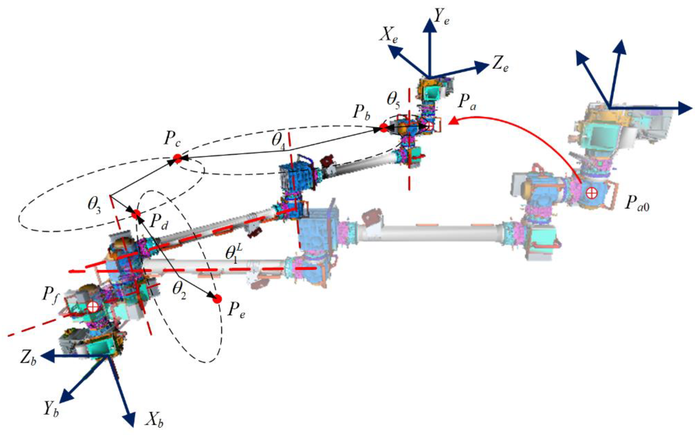
Figure 4.
The Constraint Relationship of Pd.
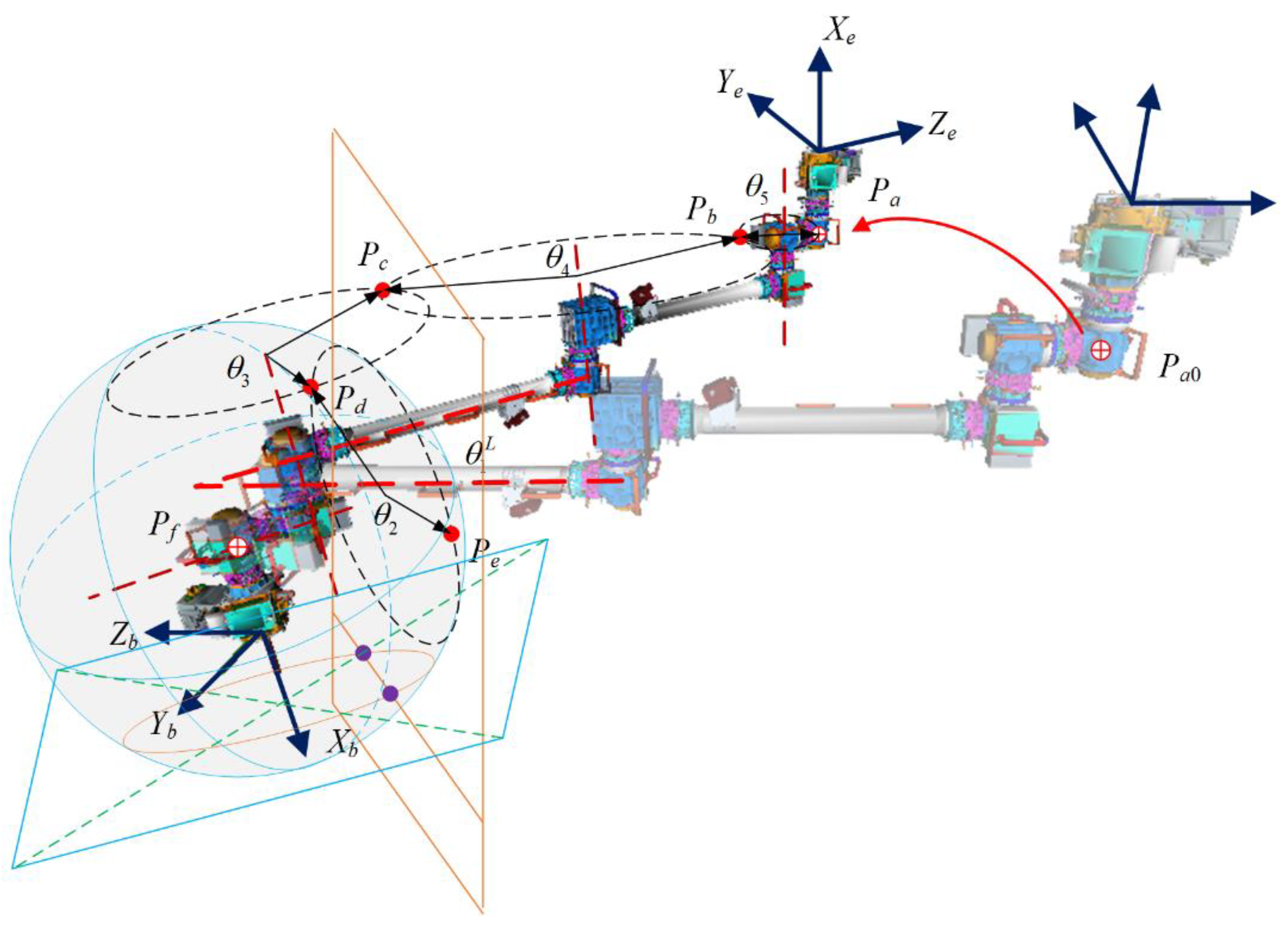
Figure 5.
Sectional View of The Cutting Plane.
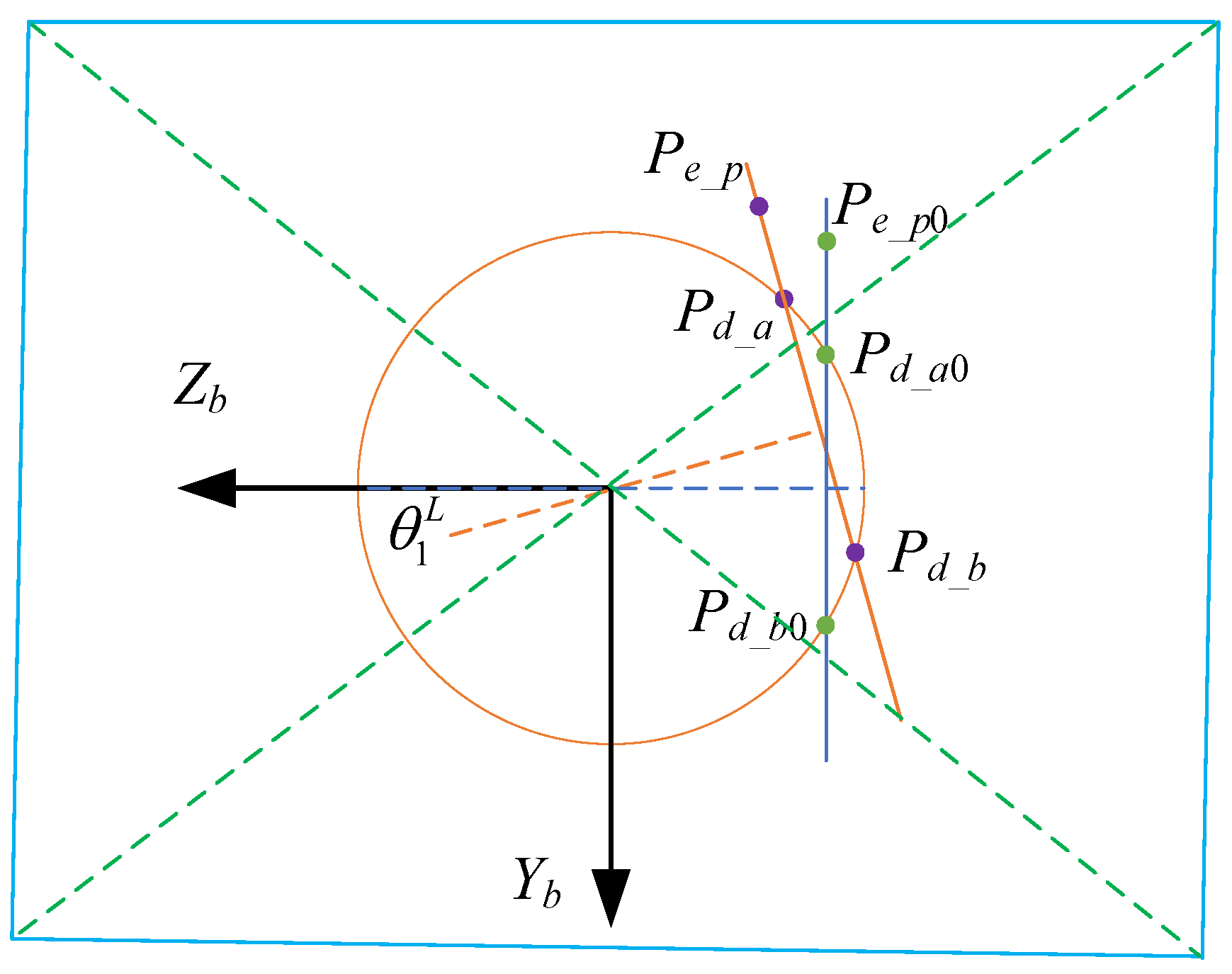
Figure 6.
Transformation of Joint 2 Angle.
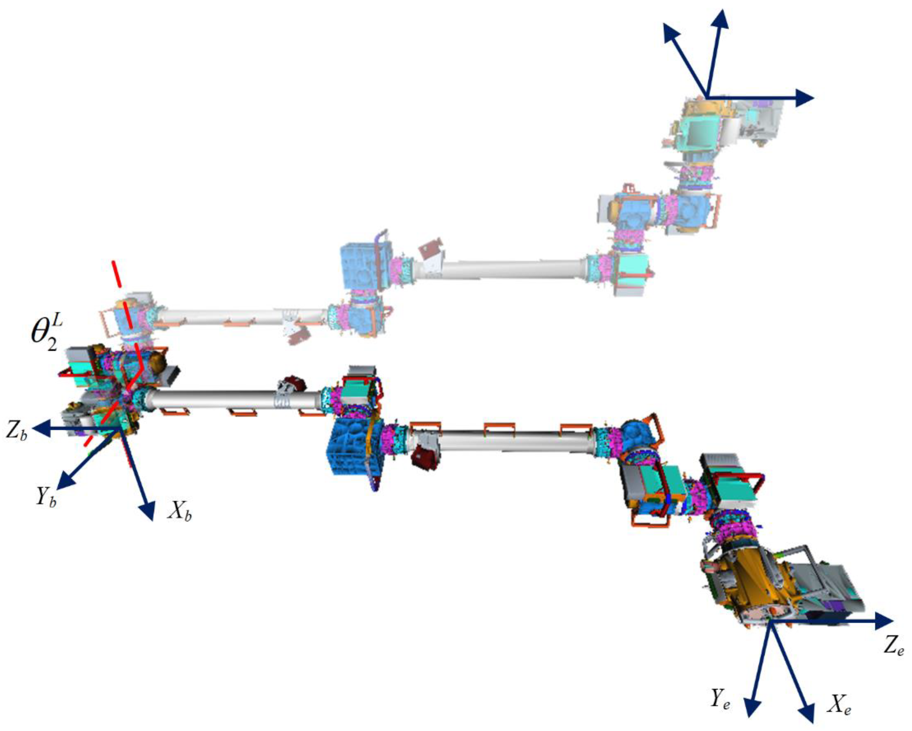
Figure 7.
Transformation of Reference Points.
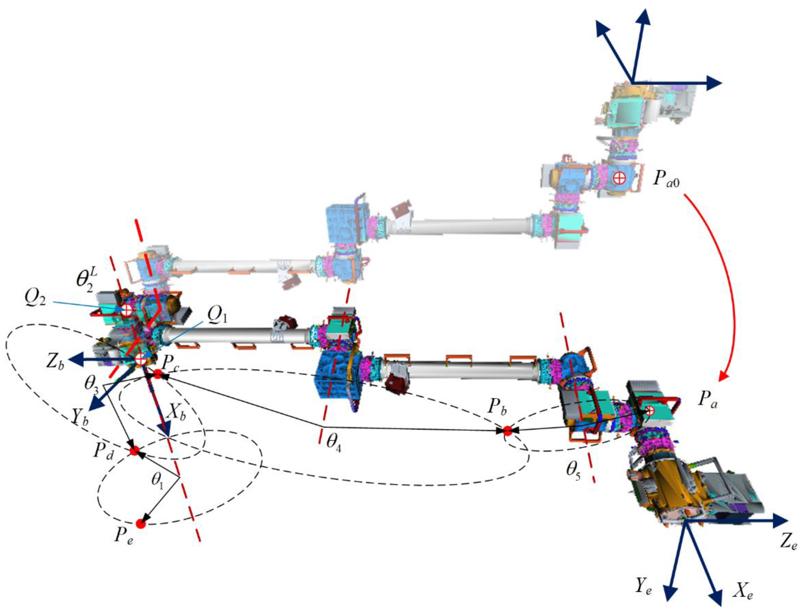
Figure 9.
Solving Capability at Different Positions.
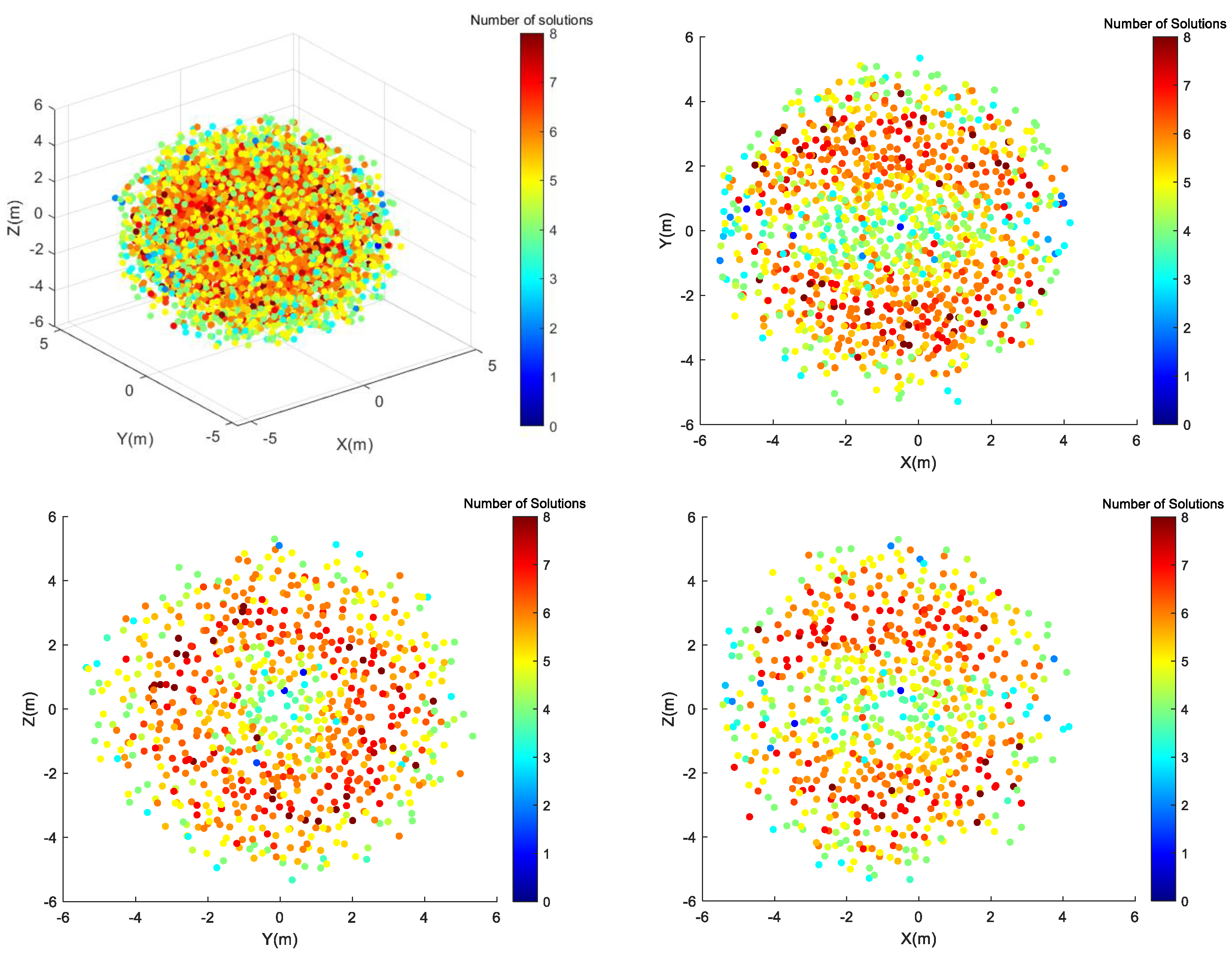
Table 2.
Definition of Joint Helical Axes.
| i | ||
| 1 | -1, 0, 0 | 0, 0, 0 |
| 2 | 0, 0, -1 | , 0, 0 |
| 3 | -1, 0, 0 | |
| 4 | -1, 0, 0 | |
| 5 | -1, 0, 0 | |
| 6 | 0, 0, -1 | , 0, 0 |
| 7 | -1, 0, 0 |
Table 3.
Coordinate of the helical Axis of the Joint.
| i | ||
| 1 | -1, 0, 0 | 0, 0, 0 |
| 2 | 0, 0, -1 | 0, , 0 |
| 3 | -1, 0, 0 | |
| 4 | -1, 0, 0 | |
| 5 | -1, 0, 0 | |
| 6 | 0, 0, -1 | 0, , 0 |
| 7 | -1, 0, 0 |
Table 4.
Statistics on the number of successful experiments and success rates.
| Joint fixation strategy | Number of successes | Success rate (%) |
| Fixed Joint 1 | 9977 | 99.77 |
| Fixed Joint 2 | 9974 | 99.74 |
| Fixed Joint 6 | 9976 | 99.76 |
| Fixed Joint 7 | 9979 | 99.79 |
| Fixed Joint 3 | 9968 | 99.68 |
| Fixed Joint 4 | 9965 | 99.65 |
| Fixed Joint 5 | 9969 | 99.69 |
Disclaimer/Publisher’s Note: The statements, opinions and data contained in all publications are solely those of the individual author(s) and contributor(s) and not of MDPI and/or the editor(s). MDPI and/or the editor(s) disclaim responsibility for any injury to people or property resulting from any ideas, methods, instructions or products referred to in the content. |
© 2026 by the authors. Licensee MDPI, Basel, Switzerland. This article is an open access article distributed under the terms and conditions of the Creative Commons Attribution (CC BY) license (http://creativecommons.org/licenses/by/4.0/).
Copyright: This open access article is published under a Creative Commons CC BY 4.0 license, which permit the free download, distribution, and reuse, provided that the author and preprint are cited in any reuse.


