
Submitted:
14 January 2026
Posted:
15 January 2026
You are already at the latest version
Abstract
This article investigates the qualification of photovoltaic micromodules intended for energy harvesting in Internet-of-Things systems, with emphasis on the degradation mechanisms induced by accelerated environmental aging typical of tropical conditions. The study employs multiple complementary characterization techniques—including pulsed I–V measurements, electroluminescence imaging, and impedance spectroscopy—combined with multivariate statistical analysis to support decision-making regarding acceptance criteria, fault prediction models, maintenance scheduling, and failure mode clustering.In addition, dimensionality-reduction methods are explored to extract the most relevant indicators from empirical datasets and to improve interpretability when dealing with highly correlated or redundant variables. The work addresses a regulatory gap affecting photovoltaic devices below 5 Wp, a class of modules whose deployment is rapidly expanding in remote, autonomous, and low-power IoT applications, yet remains largely unsupported by existing reliability and certification standards.
Keywords:
photovoltaic micro-modules
; energy harvesting
; Internet of Things (IoT)
; pulsed I–V characterization
; impedance spectroscopy
; electroluminescence imaging
; grayscale analysis
; degradation analysis
; reliability assessment
1. Introduction
Photovoltaic (PV) market has reported consistent evidence of early-stage performance losses in solar modules operating in the field, with degradation levels reaching up to 20% of the rated power under severe conditions within the first years of deployment [1]. In the context of commissioning utility-scale installations and laboratory-based quality assessment, several diagnostic techniques are widely established and routinely applied. Among them, the current–voltage (I–V) curve tracing enables the extraction of fundamental electrical parameters and the determination of peak power, whereas electroluminescence (EL) imaging is used to identify microcracks, structural degradation, and intrinsic defects in solar cells [2]. These procedures constitute consolidated methodologies for both laboratory characterization and field diagnostics of conventional PV modules.
Despite the maturity of these approaches when applied to full-scale modules, PV micromodules remain outside the scope of the current regulatory framework. Brazilian standards governing PV module qualification, the most notably INMETRO Ordinance No. 140 cover only devices with power ratings above 5 Wp. As a result, there is a technical and regulatory gap regarding the performance, reliability, and environmental behavior of low-power devices, particularly when deployed in Internet of Things (IoT) applications. This gap becomes increasingly critical considering that micromodules are frequently employed as energy-harvesting sources in systems subject to stringent size constraints, intermittent illumination, and limited power budgets. To achieve a comprehensive understanding of micromodule behavior, this work employs multiple complementary characterization techniques, including impedance spectroscopy (IS), pulsed-irradiance I–V measurements, electroluminescence imaging, and grayscale histogram analysis. Together, these techniques support robust differentiation between healthy and degraded samples and provide experimental evidence for interpreting the statistical signatures revealed by multivariate data analyses. Such interpretation contributes to advancing the current understanding of failure mechanisms in PV micromodules.
In addition, accelerated aging and reliability tests—including salt mist exposure, damp heat, and thermal cycling—were conducted to induce representative degradation modes. These environmental stress tests enable systematic evaluation of micromodule behavior under controlled stress conditions and facilitate correlating degradation mechanisms with emergent patterns identified through electrical and optical measurements. Finally, advanced statistical methods are applied to the experimental dataset, establishing an integrated data repository encompassing all characterization stages. This statistical approach enables sample classification, definition of acceptance thresholds, identification of degradation trends, and prediction of failure progression, providing an essential framework for assessing the reliability of low-power PV micromodules and can be extended to other techniques such as Transfer length method (TLM) [3,4] and reflectometria no domínio do tempo (TDR) [5,6].
2. Photovoltaic Micromodules for Energy Harvesting in IoT Systems
Advances in low-power electronic circuits and the increasing adoption of Internet of Things (IoT) devices have positioned energy harvesting as a strategic enabler for autonomous and sustainable systems. Among various ambient energy sources, solar irradiation stands out due to its high energy density and continuous availability, making it widely deployed in sensors, wireless transmitters, and embedded microcontrollers [7]. Unlike conventional photovoltaic modules, typically rated above 100 Wp and designed for centralized or distributed power generation, PV micromodules operate in much lower power ranges—from milliwatts to a few watts—and are optimized for low-irradiance operating conditions commonly encountered in indoor environments and embedded applications [8]. Energy harvesting refers to the conversion of environmental sources such as light, vibration, thermal gradients, or electromagnetic radiation into usable electrical power. Within IoT ecosystems, light energy—particularly solar—is often the most practical power source, balancing energy availability, conversion efficiency, and system-level integration simplicity [9].
2.1. Structural Differences Between Conventional Modules and PV Micromodules
Conventional photovoltaic modules incorporate bypass diodes, junction boxes, MC4 connectors, and metallic frames to ensure mechanical resilience, series current continuity, and safe operation. By contrast, PV micromodules prioritize simplicity, mass reduction, and cost efficiency, typically consisting of fragmented solar cells assembled via laminate processing but without bypass diodes, connectors, or framing. The micromodule investigated in this work consists of 10 to 12 monocrystalline fragments connected in series through a single busbar, with an active area of approximately (10.5 cm²). Under Standard Test Conditions (1000 W/m², C, AM 1.5G), nominal peak power is approximately 1.5 W. The physical dimensions of the devices are illustrated in Figure 1, and Table 1 details the sample identification and electrical parameters, as provided by the manufacturer. Both families employ bifacial Passivated Emitter and Rear Cell (PERC) technology, commonly found in compact photovoltaic devices.
Despite their advantages, micromodules exhibit higher susceptibility to partial shading and reduced thermal dissipation, owing to the absence of bypass diodes and metallic framing. However, these limitations are offset by low mass, reduced bill of materials, and straightforward integration into electronics and enclosure systems.
3. Methodology
In this work, a comprehensive experimental and analytical framework was employed to evaluate the degradation mechanisms of photovoltaic micromodules subjected to accelerated reliability stresses. Four complementary characterization techniques were applied to extract electrical and structural indicators of performance loss. Pulsed-irradiance I–V measurements were used to assess the degradation of output power and extract electrical parameters before and after environmental stress exposure. Electroluminescence (EL) imaging, combined with grayscale histogram analysis, enabled the detection of structural defects such as cracks, inactive regions, and non-uniform current flow within the devices. Electrochemical impedance spectroscopy (EIS) was implemented to extract equivalent-circuit parameters, including series resistance (), shunt resistance (), and junction capacitance (), which served as proxies for corrosion, recombination, and degradation of semiconductor interfaces. Finally, statistical and reliability tools were employed to integrate the electrical and structural measurements.
To support decision-making and interpret the large volume of data generated through these characterization steps, several multivariate and reliability techniques were applied to the combined dataset. Principal Component Analysis (PCA) enabled dimensionality reduction and visualization of degradation clustering behavior, while hierarchical clustering techniques were utilized to identify similarity groups and categorize degradation mechanisms among the tested samples. Pearson correlation analysis was conducted to quantify relationships between electrical, optical, and impedance-derived parameters. Weibull reliability modeling provided estimates of failure probabilities and characterization of degradation progression across stress levels. In addition, fuzzy logic inference was adopted to classify micromodule conditions—healthy, transitional, and degraded—accounting for measurement uncertainty and parameter variability.
Together, these procedures establish a unified methodology that integrates electrical, structural, and statistical perspectives, forming a robust analytical foundation for reliability assessment, failure precursor identification, and acceptance criteria definition for photovoltaic micromodules employed in IoT energy harvesting applications.
3.1. Sample Selection and Control Strategy
A rigorous definition of the sample population is essential for validating any qualification methodology. In this work, sample control is performed in a structured manner, covering traceability, categorization of micromodule families, separation between control and test groups, and systematic application of accelerated stress testing. This organization ensures statistical consistency and supports comparative modeling between healthy and degraded conditions. To validate the qualification methodology, a representative set of reference samples was defined. For each family (A and B), three healthy modules exhibiting nominal electrical and optical performance were selected as the control group. These units establish the baseline against which degraded samples are compared.
The remaining modules were classified as test samples and subjected to accelerated degradation procedures, including salt mist (NS), thermal cycling (CT), and damp heat (CU), each applied at controlled severity levels ranging from 1 to 4. These stressors were selected to emulate realistic degradation mechanisms affecting photovoltaic devices deployed in the field. After testing, all units—degraded and non-degraded—were re-characterized through electrical and optical methods to determine shifts in performance and defect progression relative to their initial state.
3.2. Sample Coding and Traceability
A structured coding scheme was adopted to ensure traceability, following the pattern in (1):
Where , being C = Control, M = Tested, , . Table 2 summarizes the total sample population allocated for the experiments.
4. Accelerated Degradation Testing of PV Micromodules
To evaluate the robustness and reliability of the micromodules, all samples — except those classified as controls — were subjected to accelerated environmental degradation tests in Thermotron and Vötsch climatic chambers, and in an ABMTM salt fog chamber. The objective of these tests is to induce, in a controlled manner, degradation mechanisms typically observed in fielded photovoltaic devices, particularly in tropicalized electronic systems, thus enabling direct comparison between healthy and degraded samples. All samples remained unpowered throughout the tests to ensure that observed degradation effects were caused solely by the environmental stress conditions.
4.1. Salt Mist Exposure
The neutral salt spray (NSS) test was conducted following IEC 61701 using a 5% sodium chloride (NaCl) solution in deionized water, with pH between 6.5 and 7.2, at a temperature of . Exposure times were defined per corresponding to severity levels 1 through 4, respectively. The salt mist test is designed to simulate coastal and high-salinity environments characterized by elevated humidity, suspended saline aerosols, and alternating wet–dry exposure cycles [10]. In photovoltaic modules, these environmental conditions accelerate electrochemical corrosion [11], promote ionic intrusion through the encapsulation layers [12], degrade insulation, and impair both the semiconductor/metal junction and the metallization of the cells [11].
4.2. Thermal Cycling
The thermal cycling test followed IEC 61215, Section 10.11, using a temperature range from to , with dwell times of 5 minutes at each extreme and a ramp rate of . Severity levels were defined by the number of completed cycles as corresponding to levels 1 to 4. Thermal cycling induces multiple degradation mechanisms in photovoltaic micromodules, driven by the continuous stress imposed by alternating exposure to low and high temperatures. The mismatch in thermal expansion coefficients among constituent materials leads to mechanical fatigue and progressive structural deterioration [13,14]. As stress accumulates, microcracks may form within crystalline silicon cells, increasing non-radiative carrier recombination and reducing effective charge collection [15]. Repeated contraction and expansion also induce changes at the cell–metal interface, degrading solder joints and increasing contact resistance [16]. Thermal cycling further promotes delamination and encapsulant detachment, which in turn facilitates moisture ingress and accelerates dielectric breakdown and metallization corrosion [17]. Finally, localized current crowding and hotspot formation may amplify internal heating, synchronizing thermomechanical fatigue with semiconductor degradation and compounding the overall loss of performance [18].
4.3. Damp Heat Exposure
The constant damp heat test was conducted according to IEC 61215-2, Section 10.13, at and a relative humidity of . The exposure periods are summarized in matching severity levels 1 through 4. The objective of the test is to accelerate degradation mechanisms associated with moisture ingress [19], contact corrosion [20], encapsulant delamination and material deterioration [21], as well as semiconductor junction degradation caused by ionic contamination [22], thereby simulating field conditions typical of tropical or humid environments.
4.4. Particularities and Degradation Susceptibility of PV Micromodules
PV micromodules exhibit geometrical and structural characteristics that make them inherently more susceptible to accelerated degradation when compared to conventional full-size photovoltaic modules. A primary factor is their high perimeter-to-area ratio, which results in a larger proportion of exposed edges and consequently facilitates moisture penetration and ion migration. Furthermore, these devices commonly employ thinner and less redundant encapsulation layers, meaning that EVA and backsheet structures are less robust and therefore more prone to delamination and corrosion. The compact form factor also leads to reduced spacing between solar cells and interconnects, increasing the probability of unintentional parasitic current pathways as well as elevating effective series resistance. In addition, the reduced thermal mass typical of micromodules allows temperature to rise more rapidly during operation or environmental stress, amplifying thermomechanical fatigue and accelerating degradation processes.
Approximately 50% of the evaluated micromodules exhibited measurable structural or electrical deterioration with corresponding reductions in energy generation capability. These degraded samples form the basis for the validation procedures and statistical decision models developed later in this work, enabling quantitative assessment of the methodology’s ability to reliably distinguish between healthy and degraded devices.
5. Pulsed Irradiance Characterization
The pulsed irradiance characterization was conducted before and after the accelerated degradation tests. The objective of this step is to determine the maximum power of the PV micromodules and quantify performance losses attributable to the environmental stresses applied during reliability testing [23].
5.1. Test Setup for Maximum Power Determination
The configuration comprises a class AAA solar simulator and its associated dark chamber, which provides controlled conditions for irradiance and temperature [24]. Figure 2 illustrates the experimental setup used for pulsed irradiance characterization.
The dark chamber is equipped with a calibrated reference cell and a temperature sensor, which record the effective irradiance and device temperature at the instant of the 70 ms flash pulse [27]. For the micromodules under test, fabricated using bifacial PERC (Passivated Emitter and Rear Cell) technology, no additional correction is required for parasitic capacitance, as the dynamic response of the cells is well suited to short-pulse excitation. The measurement uncertainty associated with the solar simulator is of the measured maximum power, in agreement with class AAA simulator performance requirements [28].
5.2. Failure Criterion for PV Micromodules
The adopted failure criterion establishes that a micromodule is classified as degraded when the measured maximum power, after the reliability tests, falls more than 15% below the nominal manufacturer rating. This threshold provides adequate margin to identify functionally meaningful degradation without compromising classification sensitivity. Table 3 summarizes the measured maximum power after the reliability tests, highlighting the assigned pass/fail status. After identifying the failed samples based on maximum power variation, detailed parameterization of their I–V curves was performed by comparison with the mean control response for each family. Figure 3 present normalized plots of the extracted curves.
6. Electroluminescence Imaging Inspection
Electroluminescence (EL) inspection [29] was performed for all samples before and after the accelerated degradation tests, with the objective of identifying structural defects and changes in emission that could be correlated with the electrical variations observed [30]. All measurements were performed inside a dark chamber using an infrared-sensitive camera (Canon E05) and a stabilized power supply (ITECH). Excitation conditions were kept constant throughout all experiments: bias voltage of 6 V and current of 0.25 A, values compatible with the electrical characteristics of the investigated micromodules.
Figure 4 illustrates the experimental setup implemented for EL imaging acquisition and Table 3 summarizes the parameters extracted from the EL histograms for samples after environmental stress.
6.1. Image Processing and Parameter Extraction
The analysis of electroluminescence (EL) images is a widely adopted non-destructive method employed in the characterization of photovoltaic (PV) modules. The purpose of this procedure is to extract quantitative information regarding emission intensity, spatial uniformity, and the presence of defects through grayscale conversion and subsequent statistical evaluation via grayscale histograms.
EL images are typically captured using CCD or near-infrared cameras and may be recorded in RGB format. To standardize the processing workflow, the image is converted to grayscale using the transformation defined by ITU-R BT.601 [31], as expressed in (2),
where , , and denote the pixelwise color components. The converted image assumes values within the range where 0 represents no detected emission (absolute black), and 255 corresponds to maximum recorded emission. After conversion, grayscale values are mapped into a histogram. The histogram is a function describing the frequency distribution of pixels across all gray levels, as defined in where . The histogram enables identification of regions with suppressed emission, saturation, and spatial non-uniformities in the PV micromodule.
6.2. Extraction of Statistical Parameters from the Histogram
Parameters derived from the histogram provide quantitative indicators of the emission behavior exhibited by the micromodule. The mean grayscale value provides an estimate of global emission intensity as expressed in (3),
Where M and N denote the pixel dimensions of the image. Contrast quantifies statistical variability in emission values and is given by (4),
Elevated values indicate the presence of anomalous emissive behavior such as microcracks or inactive cell regions. The maximum and minimum intensity values in the image are defined as this measurement identifies the dynamic emission range captured in the image. Using a threshold value (midpoint of the grayscale interval), the fractions of bright and dark pixels are defined in (5),
These parameters quantify the fraction of the module exhibiting meaningful emission. Global uniformity may be estimated as the ratio between dispersion and mean intensity, as shown in (6),
Values approaching unity indicate spatially uniform emission across the micromodule.
7. Complex Impedance Characterization by Impedance Spectroscopy (EIS)
The impedance spectroscopy (IS) was performed for both reference samples and those subjected to accelerated lifetime tests [32]. The objective is to track the evolution of the key parameters of the equivalent electrical circuit representing the micromodules: series resistance (), parallel resistance (), and parallel capacitance (), which serve as direct indicators of electrical and structural integrity.
7.1. EIS Measurement Setup for Photovoltaic Micromodules and Parameter Extraction from Complex Impedance
A precision Agilent E4980A LCR meter was employed, operating over a frequency range of 20 Hz to 2 MHz using a Kelvin (four-wire) connection, as shown in Figure 5. The four-wire configuration minimizes cable-related parasitic resistance, thus improving accuracy in the estimation of , particularly at low frequencies [33,34,35].
Measurements were carried out in temperature- and humidity-controlled laboratory conditions, with no DC bias applied. Unlike full-size PV modules equipped with long cabling and MC4 connectors, the micromodules tested do not exhibit inductive signatures. This absence reinforces the dominant capacitive–resistive behavior, enabling the use of a lumped-element representation for the electrical characterization [36]. Accordingly, the complex impedance of the PV module can be computed as in (7),
Where denotes the series resistance, the equivalent parallel resistance, and the equivalent parallel capacitance. This model may be simplified by grouping the electrical elements and .
The series resistance is obtained from the high-frequency limit of the impedance spectrum [37]. For , the capacitor in the parallel branch behaves as a short circuit, causing the impedance of the parallel branch to vanish, as expressed in (8),
Once is known, can be obtained from the low-frequency impedance magnitude according to (9),
Which reflects the dominance of resistive leakage and recombination-related pathways at low frequencies.
Assuming that and have already been determined. In the mid-frequency range, the impedance magnitude begins to decrease with increasing frequency due to the dominant contribution of . From this medium-frequency impedance magnitude , may be computed using (10),
This approach allows impedance parameters to be extracted solely from frequency-domain measurements without the need for illumination or external bias, enabling a fully non-destructive and contact-condition-sensitive characterization of degradation.
Physically, represents the contribution of metallic traces, ohmic resistance of internal interconnects, and the intrinsic resistive properties of the micromodule materials in the other hand the parameter is strongly related to recombination mechanisms, junction defects, and leakage current pathways within the photovoltaic device and finally this capacitance is associated with the dielectric behavior of the depletion region of the semiconductor junction.
Figure 6 show impedance curves for degraded samples contrasted against their respective reference sets. Table 3 summarize the extracted values of , , and .
Minor oscillations in the low-frequency region were attributed to instrument noise and did not significantly affect the estimation of , , and .
8. Multivariate statistical analysis
8.1. Principal Component Analysis (PCA) to Determine Covariance Between Parameters
Prior to multivariate analysis [38], all variables were standardized to eliminate scale effects, according to (11),
where is the original value of variable j for sample i, is the mean of variable j, is the standard deviation, and is the standardized value with zero mean and unit variance across the dataset. This procedure ensures equal statistical weighting of all variables, preventing those expressed in larger numerical ranges (e.g., resistance) from dominating the model.
Principal Component Analysis (PCA) is based on the spectral decomposition of the covariance matrix (or correlation matrix) derived from standardized data [39]. The covariance matrix is defined in (12),
Where is the standardized data matrix containing n samples and p variables, and is the covariance matrix describing how pairs of variables vary together. PCA requires solving the eigenvalue decomposition problem, shown in (13),
Where is the eigenvalue associated with principal component k and is the corresponding eigenvector defining the principal direction. All principal components are mutually orthogonal. Projection of the standardized data into the reduced orthogonal space is obtained from (14),
Where is the PCA scores matrix (coordinates of samples in the new basis) and contains the eigenvectors as columns. Each row of contains the PC1, PC2 and PC3 values of a given sample [40]. The variance explained by each component is computed using (15),
Meaning that PC1, PC2 and PC3 capture the three dominant directions of variation in the dataset. Their physical interpretation is summarized in Table 4.
Figure 7 a) shows the three-dimensional projection of the samples in the first three principal components (PC1=42.40%, PC2=17.72%, PC3=12.72%), collectively accounting for 72.84% of the total variance.
Thus, PCA separates samples based on their multivariate signatures, enabling discrimination between “Reference”, “Approved”, “Failed”, and “Degraded” groups for each pattern. For each group, the centroid in PCA space is calculated using (16),
Where is the number of samples in group g. The Euclidean distance between two centroids and is defined in (17),
Providing a quantitative measure of dissimilarity between classes and indicating how strongly sample groups diverge statistically. Centroids were computed in the three-dimensional PCA space, and pairwise Euclidean distances were obtained, as shown in Table 5 and Table 6.
Distances confirm a clear separation between failed samples and all other groups. Each original variable contributes to PC1, PC2 and PC3 according to its loading coefficients . The overall importance of each variable in the 3D PCA model is given in (18),
Where represents the total contribution of variable i to the variance explained by the first three principal components. This weighting indicates the relative influence of each parameter on the statistical separation of samples. Figure 7 b) highlights the ten most influential variables and Figure 7 c) illustrates the contribution of each eigenvector in euclidean space. The length of each loading vector reflects its contribution to total variance, expressed in (19),
While the angle between two vectors approximates their correlation, given in (20),
With the angle of °being strongly directly related, the angle of 0°being independent, and the angle of °being strongly inversely related. Finally, the correlation heatmap encodes the Pearson correlation coefficient r between variable pairs, defined in (21),
Figure 8 shows the heatmap summarizing linear correlations.
The plot therefore acts as a statistical x-ray of the experimental dataset, illustrating how measured quantities evolve jointly — reinforcing whether they increase together, diverge in opposite directions, or evolve independently.
8.2. Fuzzy-Logic Decision Methodology for Qualification of PV Micromodules Based on Empirical Data
The fuzzy logic system developed [41] in this work is designed to evaluate the degradation state of photovoltaic micromodules based on experimentally measured electrical and optical parameters, compared against reference (control) samples. The output of the system is a fuzzy performance index (score) ranging from 0 to 100, which is subsequently categorized into one of four decision classes: Approved, Upper Boundary Approved, Lower Boundary Failed, and Failed.
Mathematically, each fuzzy input variable x belongs to a linguistic set A according to a membership function defined in where indicates nonmembership, full membership, and intermediate values indicate partial membership. The fuzzy inputs are derived from three major groups of measurements applied to the PV micromodules, and the model employs nine primary input variables grouped by physical domain, namely: (a) Electrical Domain (Photoconversion) – Pulsed I–V curve measurements, summarized in this term represents the photovoltaic performance extracted from pulsed I–V measurements, (b) Electrical Domain (RLC Charge and Transport) from Impedance Spectroscopy, as shown in which incorporates changes in series and shunt resistance and parallel capacitance extracted from the complex impedance response and (c) Optical Domain – Electroluminescence (Image-Based Metrics), as given in where is the mean gray-level emission, the image contrast (standard deviation), and U the optical uniformity, all extracted from grayscale histograms of EL images.
For each input variable , the deviation relative to the mean of the control group within the same family (A or B) is computed according to (22),
These deviations are normalized to the interval using (23),
where is the observed value, the control mean, and avoids division by zero.
Thus, smaller normalized values indicate better performance (lower degradation). Each input variable is then mapped to three linguistic fuzzy sets defined in . Triangular membership functions are applied according to (24), (25), and (26),
Standardized values used in this study are given in . Fuzzy inference rules were derived from expert knowledge [42]. For each measurement block (IV, IS, and EL), a Mamdani system [43] was constructed using rules such as (27)–(),
The inference engine aggregates rule outputs using the min–max composition operator (30),
Each fuzzy subsystem is defuzzified using the centroid method (31),
Yielding three normalized subsystem scores . The global fuzzy score is computed via a weighted sum (32),
S ubject to . The weighting factors are determined by supervised optimization to maximize agreement with expert ground-truth decisions (“Pass” / “Fail”), according to (33),
Where T is an optimally determined decision threshold. A fuzzy tolerance region with width is then defined following (34),
The fuzzy methodology therefore correlates electrical and optical deviations ( parameter variations) with the degree of functional degradation of the micromodules, effectively modeling expert reasoning processes and enabling interpretable, physics-informed automated decision making.
Application of the Fuzzy method to the empirical database obtained in the laboratory resulted in the graphs shown in Figure 9.
This method aims to optimize the decision criterion regarding the health state of the micromodules by combining multiple parameters in a nonlinear yet interpretable manner. Fuzzy logic provides a more realistic alternative to binary decision-making, allowing the incorporation of inherent uncertainties in experimental characterization and yielding a judgment more consistent with the gradual physical behavior associated with degradation of photovoltaic devices.
9. Failure Prediction Models for Reliability Stress Testing
The proposed framework is grounded in reliability theory [44], applied statistics, and nonlinear modeling, with the goal of describing the temporal evolution of electrical degradation, quantifying prediction uncertainties, and estimating cumulative failure probabilities [45]. Consider a set of N photovoltaic devices subjected to an accelerated reliability test characterized by elevated temperature and high relative humidity. For each device i, the maximum power point value is measured at discrete instants .
The variable of interest is defined as the relative degradation of the maximum power point, expressed as a percentage according to (35),
Where represents the mean reference power obtained from non-degraded devices or initial measurements. This normalization eliminates dependence on absolute power values and enables comparison among samples with different nominal ratings.
The degradation induced by reliability testing is a cumulative process associated with physical mechanisms. These mechanisms exhibit monotonic and irreversible behavior, which can be effectively represented by asymptotic growth functions. Therefore, a two-parameter Weibull function is adopted as a phenomenological degradation model, shown in (36),
Where is the scale parameter (characteristic time), is the shape parameter, associated with the dominant failure mechanism and denotes the expected degradation value as a function of time. Values indicate rapid early degradation followed by stabilization, corresponds to exponential decay, and identifies accelerated degradation typical of cumulative damage mechanisms. The observed degradation is decomposed as in (37),
Where represents a random term capturing measurement noise, manufacturing variability, and experimental fluctuations. It is assumed that with constant variance . Parameters and are estimated by minimizing the sum of squared residuals according to (38),
The optimization problem is nonlinear and nonconvex. Thus, the Nelder–Mead simplex algorithm is employed, which does not require explicit derivative computation and is particularly suited for small datasets and highly nonlinear response surfaces [46]. Model quality is evaluated using the root-mean-square error (RMSE), defined in (39),
RMSE provides a global measure of residual dispersion and is used as an empirical estimate of the model error standard deviation . Given the limited number of samples, uncertainty is quantified using nonparametric bootstrap resampling. Let denote the original data set. A total of B bootstrap sets , , are generated via sampling with replacement. For each bootstrap set, parameters are estimated according to (40),
A functional failure threshold is defined, associated with the maximum acceptable loss of performance. The characteristic failure time is obtained from the implicit solution of when an analytical solution is not feasible, numerical interpolation over the fitted curve is used. Assuming normally distributed residuals, the cumulative probability of failure as a function of time is calculated using (43),
Where denotes the cumulative distribution function of the standard normal law. This formulation enables the transition from deterministic degradation trajectories to probabilistic reliability metrics, which is essential for risk analysis and the establishment of qualification criteria. Figure 12, Figure 10, and Figure 11 present the Weibull fitting results for the damp heat (CU), salt mist (NS), and thermal cycling (CT) experiments, respectively, including model residuals and cumulative failure probabilities.
10. Discussion of the results
This section integrates the experimental evidence obtained from I–V curves, electroluminescence (EL), impedance spectroscopy (IS), PCA and Fuzzy inference, establishing a comprehensive interpretation of the degradation effects induced by accelerated environmental aging.
10.1. Implications from Impedance Spectroscopy
The IS results reveal systematic and physically interpretable variations in the extracted lumped parameters , , and , confirming that micromodules behave as compact R–C networks whose characteristics evolve with environmental stress.
An increase in series resistance is consistently observed across all degradation routes. This parameter reflects resistive losses associated with contact corrosion, microcracks forming in metallization pathways, and partial loss of electrical continuity. Such defects degrade current conduction and lead to power loss, particularly under higher operating currents.
Conversely, reductions in parallel resistance indicate the emergence of leakage paths or shunt channels, which may arise from moisture-driven ionic transport, encapsulant breakdown or semiconductor junction degradation. The accompanying decrease in parallel capacitance suggests changes in space-charge region dynamics and dielectric properties at the p–n junction, potentially involving defect generation, recombination center formation or depletion region widening.
Because measurements are performed under zero DC bias, diffusion-related components remain nearly constant, meaning observed changes are directly attributable to structural and electrochemical degradation. This reinforces the diagnostic role of IS as a complementary method to I–V and EL.
10.2. Multivariate Interpretation via PCA
Principal Component Analysis consolidates electrical, optical and impedance metrics into a low-dimensional space that highlights natural sample separability. Reference samples cluster distinctly by family, which validates the sensitivity of the parameters to manufacturing differences such as number of cells, contact layout and lamination design.
Approved samples form a compact grouping near reference centroids, confirming mechanical and electrical stability even after stress exposure. Degraded samples, however, distribute broadly across PCA axes, evidencing multiple independent pathways of degradation that alter different subsets of variables.
Salt mist tends to shift samples along axes dominated by , pixel-level asymmetry and minimum optical intensity, where corrosion plays a central role. Damp heat more strongly influences impedance terms and , corresponding to humidity-induced junction damage. Thermal cycling drives dispersion along dimensions tied to FF and EL uniformity, consistent with microcrack growth and fatigue.
The existence of outliers — approximately 12.5% — emphasizes transitional states in which degradation mechanisms coexist or have not yet manifested fully observable consequences.
10.3. Classification Behavior Based on Fuzzy Logic
The Fuzzy inference system aggregates the multidomain dataset into a unified degradation index, ranging from 0 to 100. Unlike traditional threshold-based qualification, Fuzzy classification introduces boundary regions that acknowledge gradual material failure, measurement uncertainty, and ambiguous conditions between “healthy” and “failed” states.
The classification map exhibits high coherence with stress severity. Mild exposures (NS1, CT1, CU1) cluster in green or blue regions, indicating retained functional capability. Intermediate severities migrate into yellow zones, marking incipient degradation that is detectable but not yet critical. Severe conditions (NS4, CU4) map predominantly into red, confirming irreversible failure signatures.
Over 90% agreement with expert evaluation underscores the applicability of Fuzzy classification for automated testing pipelines and digital factory environments. The model architecture is extendable to additional characterization domains such as thermography or time-domain reflectometry.
10.4. Reliability Modeling Through Weibull Fits
Weibull degradation models fitted to from CT, CU and NS tests provide quantitative insight into failure kinetics. In all three cases, the shape parameter indicates wear-out behavior dominated by early-stage defects, followed by progressive stabilization. This pattern is consistent with initiation and propagation phases typical of photovoltaic degradation.
Thermal cycling exhibits the smallest variance (), reflecting relatively uniform mechanical stress and microcrack formation. Damp heat introduces larger dispersion () stemming from moisture diffusion, encapsulant swelling, and semiconductor surface reactions. Salt mist yields the most variable outcome (), driven by electrochemical corrosion, metallization loss and ion transport, which occur at different rates across samples.
The Weibull framework therefore captures both the nonlinearity and the saturation tendency of degradation and offers interpretable metrics that correlate with physical mechanisms. These reliability indicators provide a foundation for lifetime prediction, useful to IoT deployments where maintenance or replacement access may be impractical.
10.5. Summary of Integrated Findings
Overall, the results demonstrate that the multimodal diagnostic methodology applied in this study is capable of:
- differentiating device families and construction types,
- identifying degradation signatures at early stages,
- detecting multiple concurrent failure mechanisms,
- providing continuous rather than binary health classification,
- generating interpretable lifetime models from accelerated aging data.
The integration of electrical, optical, impedance and statistical methodologies reveals a coherent picture of degradation pathways and establishes a consistent technical basis for qualifying PV micromodules in emerging IoT applications.
11. Conclusions
This work presented the development and validation of an innovative methodology for the qualification of photovoltaic micromodules (PV) based on statistical signatures extracted through multivariate analyses, capable of emulating the expert assessment typically required in laboratory evaluation.
The samples, grouped into Families A and B, were organized into control and test subsets to ensure traceability and statistical consistency throughout the study. Initial characterization using pulsed I–V curves, electroluminescence imaging, and impedance spectroscopy established the baseline condition of the devices, enabling direct comparison with the degradation effects induced by accelerated stress tests, including salt mist, damp heat, and thermal cycling.
The results demonstrate that the proposed methodology is a promising, sensitive, and reproducible approach for diagnosing and classifying photovoltaic micromodules. The method contributes significantly to the scientific and technological advancement of photovoltaic reliability engineering and opens new perspectives for the standardization and modernization of qualification practices applicable to miniaturized PV devices used in emerging energy-harvesting and IoT applications.
References
- Equipment, V.P. International technology roadmap for photovoltaic (ITRPV). Results 2020 2021, 12. [Google Scholar]
- Köntges, M.; Kurtz, S.; Packard, C.; Jahn, U.; Berger, K.A.; Kato, K.; Friesen, T.; Liu, H.; Van Iseghem, M.; Wohlgemuth, J.; et al. Review of failures of photovoltaic modules. 2014. [Google Scholar]
- da Silveira, A.M.; Brasil, G.T.; de Melo, W.R.; Peruzzi, V.V.; Finco, S.; Manera, L.T. Characterization of Specific Contact Resistivity in Commercial Bifacial Solar Cell Contact Electrodes: TLM Measurement Approach. Proceedings of the 2025 39th Symposium on Microelectronics Technology and Devices (SBMicro). IEEE 2025, Vol. 1, 1–4. [Google Scholar]
- Silveira, A.; Neves, M.; Garcia, R.; Alvarez, H.; Villalva, M.; Marques, F.; Kretly, L. Evolution of Metallic Connection Technologies of Busbar in Silicon Solar Cells: Brief Review. In Proceedings of the 2023 15th IEEE International Conference on Industry Applications (INDUSCON), 2023; IEEE; pp. 690–695. [Google Scholar]
- Silveira, A.; Barbin, S.; Kretly, L. Using TDR-Time Domain Reflectometry Measurements to Compare Ribbon Busbar versus Wire Busbar Connections in Polycrystalline Solar Cells: The Signature Approach. In Proceedings of the 2018 IEEE-APS Topical Conference on Antennas and Propagation in Wireless Communications (APWC), 2018; IEEE; pp. 1–3. [Google Scholar]
- Silveira, A.; Neves, M.; Garcia, R.; Alvarez, H.; Villalva, M.; Marques, F.; Kretly, L. Characterization of solar cell busbar grid for different technologies by time domain reflectometry simulation: Transmission line approach. In Proceedings of the 2023 IEEE 50th Photovoltaic Specialists Conference (PVSC), 2023; IEEE; pp. 1–5. [Google Scholar]
- Rincón-Mora, G.A.; Vogt, J. Self-powered wireless sensor nodes: Among other things, a load management feat. Power Management Des. Line 2007. [Google Scholar]
- Sarker, M.R.; Riaz, A.; Lipu, M.H.; Saad, M.H.M.; Ahmad, M.N.; Kadir, R.A.; Olazagoitia, J.L. Micro energy harvesting for IoT platform: Review analysis toward future research opportunities. Heliyon 2024, 10. [Google Scholar] [CrossRef] [PubMed]
- Tsenempis, I.; Filios, G.; Katsidimas, I.; Nikoletseas, S. Energy harvesting and smart management platform for low power IoT systems. In Proceedings of the 2019 15th International Conference on Distributed Computing in Sensor Systems (DCOSS), 2019; IEEE; pp. 339–346. [Google Scholar]
- Neves, M.R.; Silveira, A.; Alvarez, H.S.; Garcia, R.M.; Marques, F.C.; Villalva, M.G. Effects of Salt Spray on c-Si Photovoltaic Modules in the Brazilian Region. In Proceedings of the 2023 IEEE 50th Photovoltaic Specialists Conference (PVSC), 2023; IEEE; pp. 1–6. [Google Scholar]
- Rana, Z.; Zamora, P.P.; Soliz, A.; Soler, D.; Reyes Cruz, V.E.; Cobos-Murcia, J.A.; Galleguillos Madrid, F.M. Solar Panel Corrosion: A Review. International Journal of Molecular Sciences 2025, 26, 5960. [Google Scholar] [CrossRef]
- Mohamed, B.; Zambou, S.; Zekeng, S.S. Influence of moisture on the operation of a mono-crystalline based silicon photovoltaic cell: A numerical study using SCAPS 1 D. arXiv 2017, arXiv:1712.08117. [Google Scholar] [CrossRef]
- Chen, X.; Karin, T.; Jain, A. Analyzing the impact of design factors on solar module thermomechanical durability using interpretable machine learning techniques. Applied Energy 2025, 377, 124462. [Google Scholar] [CrossRef]
- Aoki, Y.; Okamoto, M.; Masuda, A.; Doi, T. Module performance degradation with rapid thermal-cycling. Proceedings of Renewable Energy; 2010. [Google Scholar]
- Park, S.; Han, C. Analysis of EL images on Si solar module under thermal cycling. Journal of Mechanical Science and Technology 2022, 36, 3429–3436. [Google Scholar] [CrossRef]
- Pandey, S.; Kumar, S.; Mhatre, R.; Singh, T. Analysis of performance degradation of PV modules. Available online: https://www. powermag. com/analysis-of-performance-degradation-of-pv-modules/ (accessed on: 30.09. 2024). 2023.
- Aghaei, M.; Fairbrother, A.; Gok, A.; Ahmad, S.; Kazim, S.; Lobato, K.; Oreski, G.; Reinders, A.; Schmitz, J.; Theelen, M.; et al. Review of degradation and failure phenomena in photovoltaic modules. Renewable and Sustainable Energy Reviews 2022, 159, 112160. [Google Scholar] [CrossRef]
- Rahman, T.; Mansur, A.A.; Hossain Lipu, M.S.; Rahman, M.S.; Ashique, R.H.; Houran, M.A.; Elavarasan, R.M.; Hossain, E. Investigation of degradation of solar photovoltaics: A review of aging factors, impacts, and future directions toward sustainable energy management. Energies 2023, 16, 3706. [Google Scholar] [CrossRef]
- Irikawa, J.; Hashimoto, H.; Kanno, H.; Taguchi, M. Correlation between damp-heat test and field operation for electrode corrosion in photovoltaic modules. Solar Energy Materials and Solar Cells 2025, 284, 113375. [Google Scholar] [CrossRef]
- Park, H.; So, W.; Kim, W.K. Performance evaluation of photovoltaic modules by combined damp heat and temperature cycle test. Energies 2021, 14, 3328. [Google Scholar] [CrossRef]
- Karin, T.; Jones, C.B.; Jain, A. Photovoltaic climate zones: The global distribution of climate stressors affecting photovoltaic degradation. In Proceedings of the Proc. 36th Eur. Photovolt. Sol. Energy Conf. Exhib. (EUPVSEC) pp, 2020; pp. 825–834. [Google Scholar]
- Deibel, C.; Dyakonov, V.; Parisi, J. Spectroscopy of electronic defect states in Cu (In, Ga)(S, Se) 2-basedheterojunctions and Schottky diodes under damp-heat exposure. Europhysics Letters 2004, 66, 399. [Google Scholar] [CrossRef]
- El Amrani, A.; Mahrane, A.; Moussa, F.; Boukennous, Y. Solar module fabrication. International Journal of Photoenergy 2007, 2007, 027610. [Google Scholar] [CrossRef]
- Serreze, H.B.; Little, R.G. Large area solar simulators–critical tools for module manufacturing. Photovoltaics International 2008, 1, 108–111. [Google Scholar]
- Dingpu, L.; Limin, X.; Haifeng, M.; Yingwei, H.; Jieyu, Z. Research on Outdoor Testing of Solar Modules. Proceedings of the Proc. of SPIE Vol 2012, Vol. 8419, 84193E–1. [Google Scholar]
- Luciani, S.; Coccia, G.; Tomassetti, S.; Pierantozzi, M.; Di Nicola, G.; et al. Use of an indoor solar flash test device to evaluate production loss associated to specific defects on photovoltaic modules. International Journal of Design & Nature and Ecodynamics 2020, 15, 639–646. [Google Scholar]
- Roy, J.; Gariki, G.R.; Nagalakhsmi, V. Reference module selection criteria for accurate testing of photovoltaic (PV) panels. Solar Energy 2010, 84, 32–36. [Google Scholar] [CrossRef]
- Georgescu, A.; Damache, G.; Girtu, M. Class A small area solar simulator for dye-sensitized solar cell testing. J. Optoelectron. Adv. Mater 2008, 10, 3003–3007. [Google Scholar]
- Fuyuki, T.; Kondo, H.; Yamazaki, T.; Takahashi, Y.; Uraoka, Y. Photographic surveying of minority carrier diffusion length in polycrystalline silicon solar cells by electroluminescence. Applied Physics Letters 2005, 86. [Google Scholar] [CrossRef]
- Hofierka, J.; Kaňuk, J. Assessment of photovoltaic potential in urban areas using open-source solar radiation tools. Renewable energy 2009, 34, 2206–2214. [Google Scholar] [CrossRef]
- International Telecommunication Union. Recommendation ITU-R BT.601-7; Studio encoding parameters of digital television for standard 4:3 and wide-screen 16:9 aspect ratios. 2011.
- Lazanas, A.C.; Prodromidis, M.I. Electrochemical impedance spectroscopy—a tutorial. ACS Measurement Science Au 2023, 3, 162–193. [Google Scholar] [CrossRef] [PubMed]
- Kumar, R.A.; Suresh, M.; Nagaraju, J. Measurement of AC parameters of gallium arsenide (GaAs/Ge) solar cell by impedance spectroscopy. IEEE Transactions on Electron Devices 2001, 48, 2177–2179. [Google Scholar] [CrossRef]
- Mueller, R.L.; Wallace, M.T.; Iles, P. Scaling nominal solar cell impedances for array design. Proceedings of the Proceedings of 1994 IEEE 1st World Conference on Photovoltaic Energy Conversion-WCPEC (A Joint Conference of PVSC, PVSEC and PSEC) 1994, Vol. 2, 2034–2037. [Google Scholar]
- Pierret, R.F. Semiconductor Device Fundamentals; Addison-Wesley Publishing Company, 1996. [Google Scholar]
- Chenvidhya, D.; Kirtikara, K.; Jivacate, C. PV module dynamic impedance and its voltage and frequency dependencies. Solar Energy Materials and Solar Cells 2005, 86, 243–251. [Google Scholar] [CrossRef]
- Kim, K.A.; Xu, C.; Jin, L.; Krein, P.T. A dynamic photovoltaic model incorporating capacitive and reverse-bias characteristics. IEEE Journal of photovoltaics 2013, 3, 1334–1341. [Google Scholar] [CrossRef]
- Jolliffe, I.T.; Cadima, J. Principal component analysis: a review and recent developments. Philosophical transactions of the royal society A: Mathematical, Physical and Engineering Sciences 2016, 374, 20150202. [Google Scholar] [CrossRef]
- Jackson, J.E. A user’s guide to principal components; John Wiley & Sons, 2005. [Google Scholar]
- Williams, L.; et al. Principal component analysis; Wiley Interdisciplinary Reviews: Computational Statistics, 2010. [Google Scholar]
- Zadeh, L.A. Fuzzy sets. Information and control 1965, 8, 338–353. [Google Scholar] [CrossRef]
- Ross, T.J. Fuzzy logic with engineering applications; John Wiley & Sons, 2005. [Google Scholar]
- Mamdani, E.H. Application of fuzzy algorithms for control of simple dynamic plant. Proceedings of the Proceedings of the institution of electrical engineers. IET 1974, Vol. 121, 1585–1588. [Google Scholar] [CrossRef]
- Weibull, W. A statistical distribution function of wide applicability. Journal of applied mechanics 1951. [Google Scholar] [CrossRef]
- Lawless, J.F. Statistical models and methods for lifetime data; John Wiley & Sons, 2011. [Google Scholar]
- Fisher, R.A.; Tippett, L.H.C. Limiting forms of the frequency distribution of the largest or smallest member of a sample. In Proceedings of the Mathematical proceedings of the Cambridge philosophical society; Cambridge University Press, 1928; Vol. 24, pp. 180–190. [Google Scholar]
Figure 1.
a) Physical dimensions of the micromodules (from datasheet); b) perspective view; c) rear view; d) EL image of a healthy Family A unit; e) EL image of a healthy Family B unit.
Figure 1.
a) Physical dimensions of the micromodules (from datasheet); b) perspective view; c) rear view; d) EL image of a healthy Family A unit; e) EL image of a healthy Family B unit.
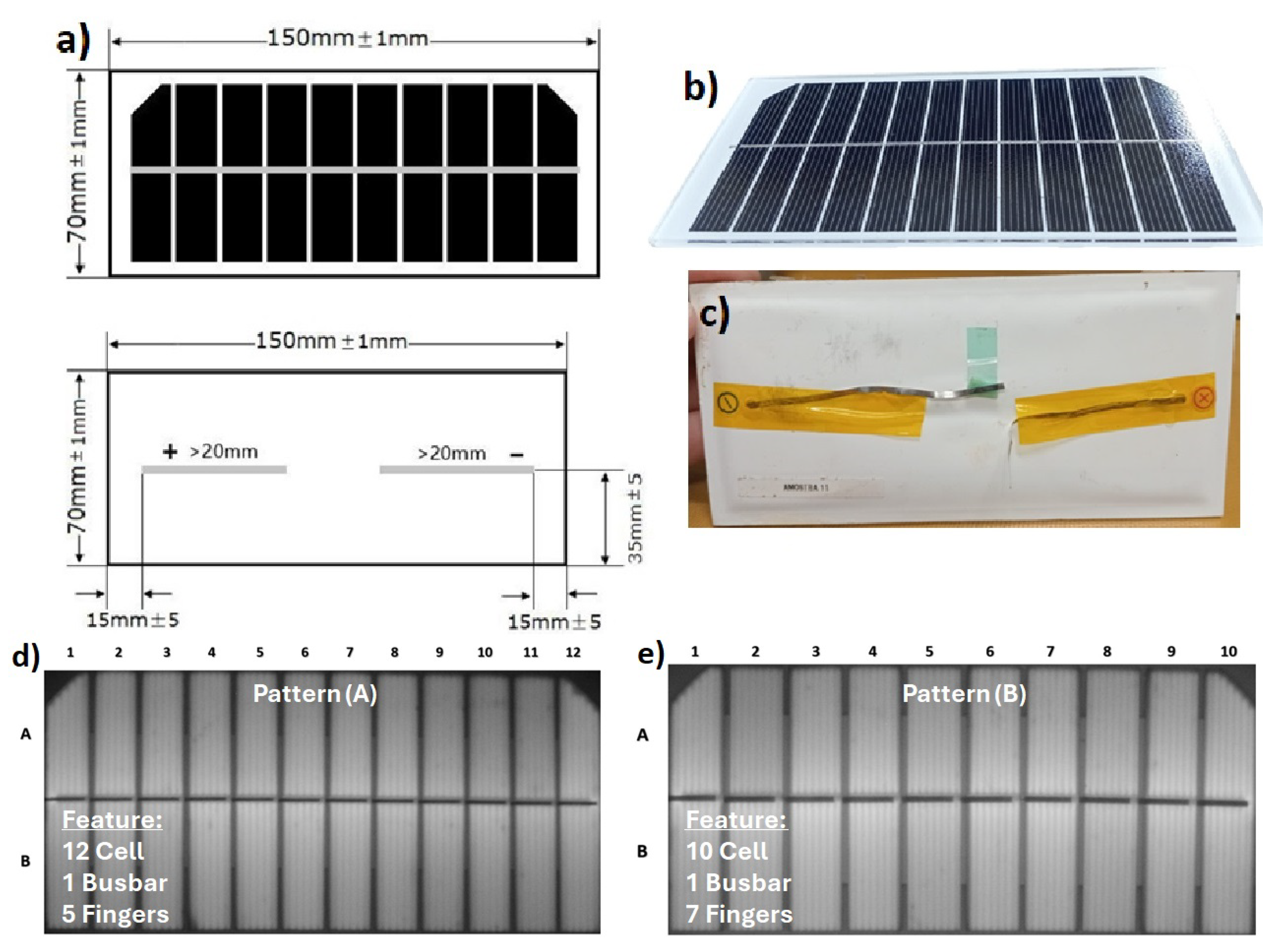
Figure 2.
a) Test setup for pulsed-irradiance measurements applied to PV micromodules; b) dark chamber of the class AAA solar simulator (Gsola model); c) schematic representation of the standard solar simulator used for I–V analysis; d) standard dark chamber configuration for assessing the spatial irradiance uniformity over the sample surface [Adapted from [25,26].
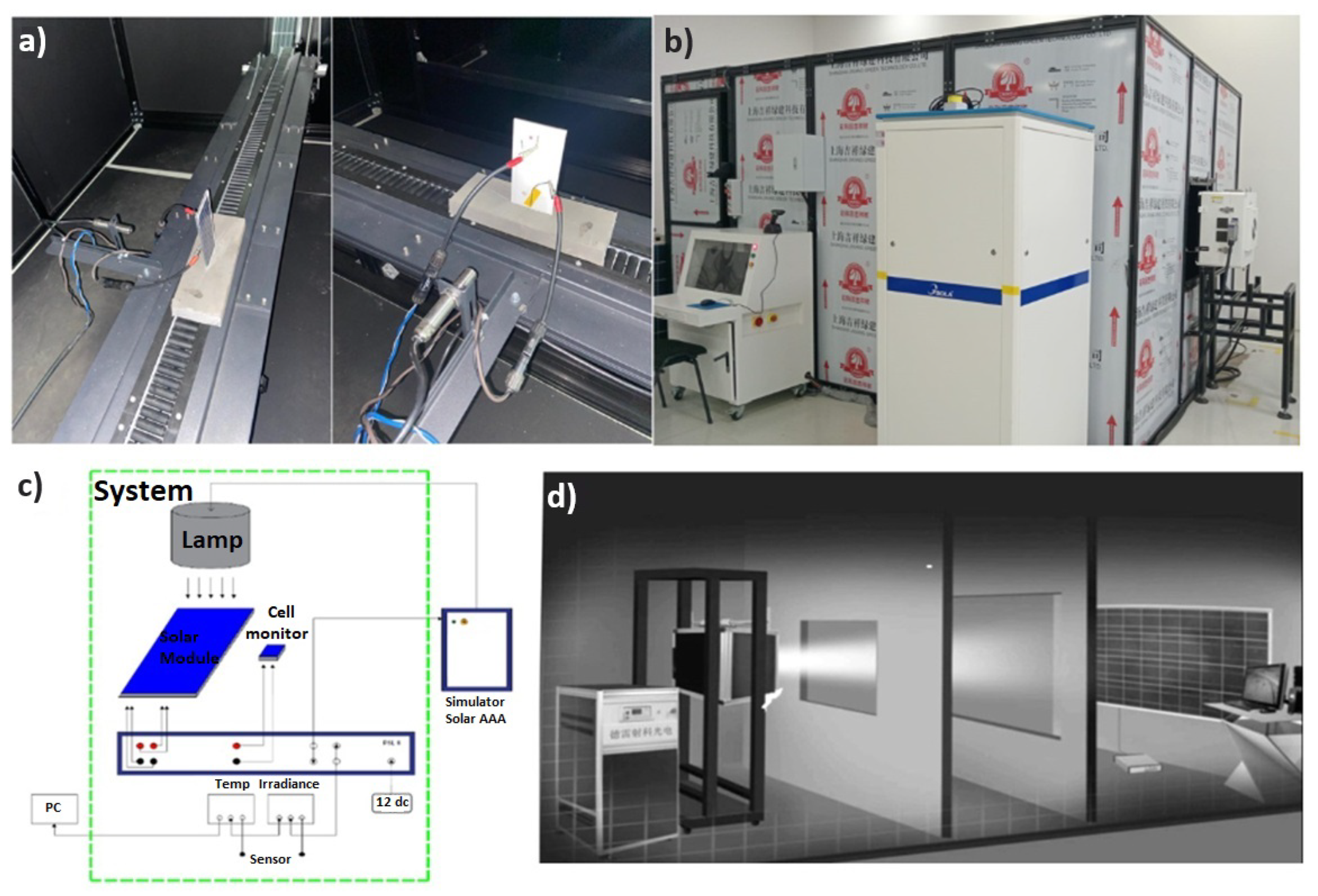
Figure 3.
Normalized parametrized I–V curves of failed samples from a) family A and b) family B compared against the average of control samples.
Figure 3.
Normalized parametrized I–V curves of failed samples from a) family A and b) family B compared against the average of control samples.
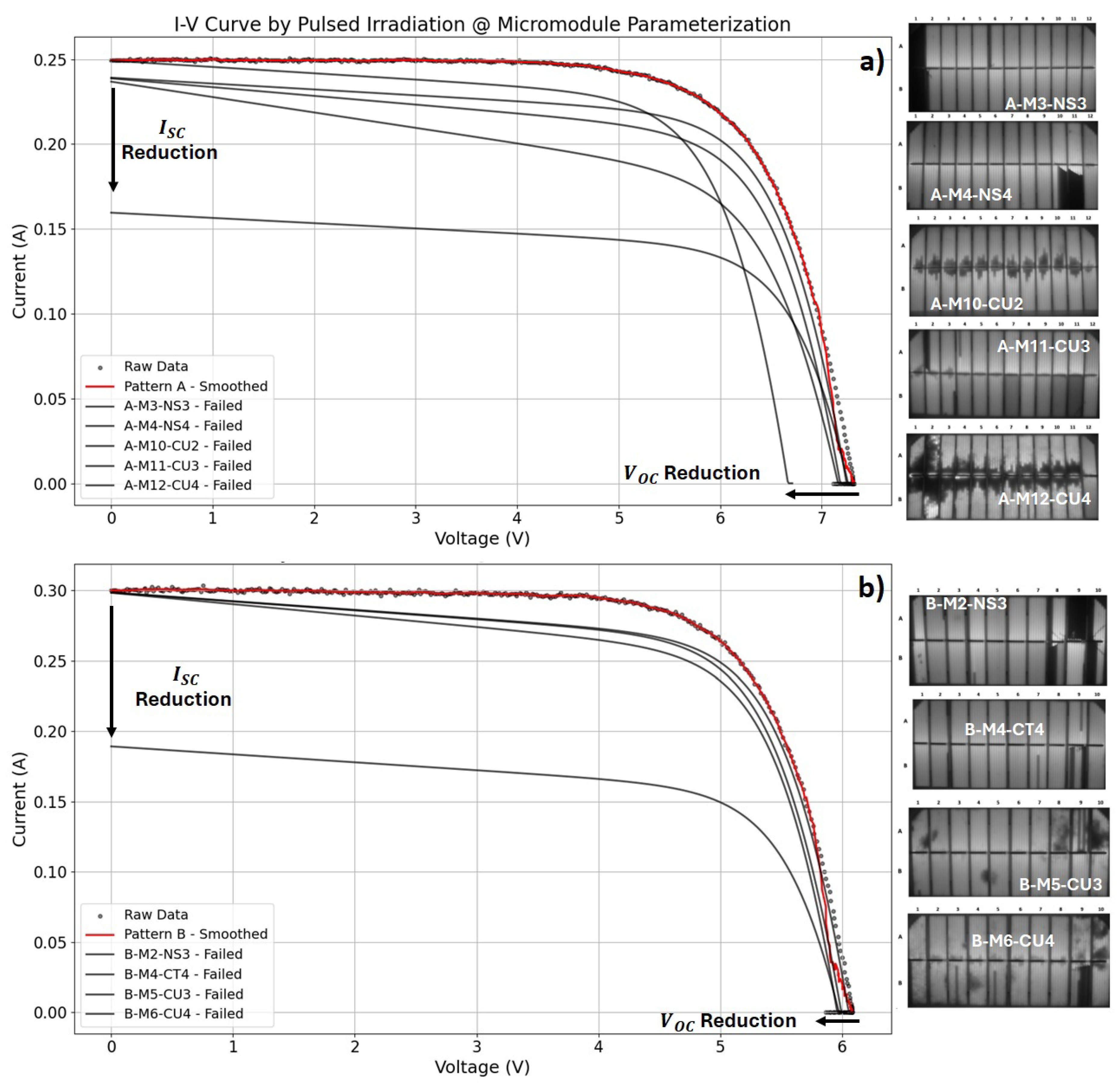
Figure 4.
a) Test setup for electroluminescence inspection; b) EL image acquisition during device excitation; c) Illustration of the test setup for obtaining the EL image [adapted from [2] and d) Illustration of the electroluminescence image inspection and its grayscale histogram performed for all micromodule samples
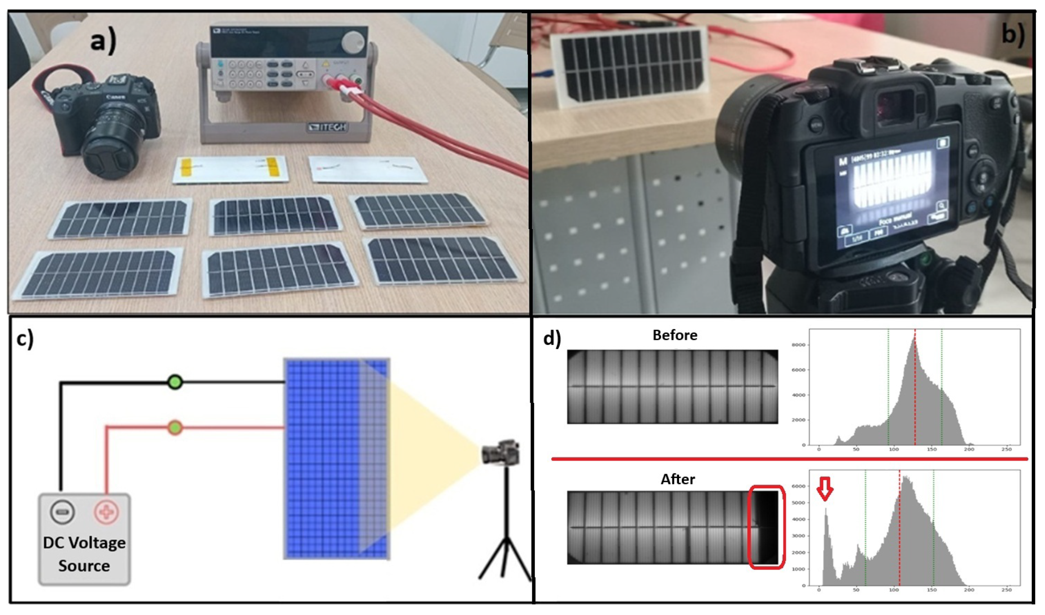
Figure 5.
a) Impedance spectroscopy setup for PV micromodules. b) Equivalent PV model under dark conditions used for frequency-domain interpretation.
Figure 5.
a) Impedance spectroscopy setup for PV micromodules. b) Equivalent PV model under dark conditions used for frequency-domain interpretation.

Figure 6.
Complex impedance of degraded samples of a) Family A and b) Family B compared to the reference.
Figure 6.
Complex impedance of degraded samples of a) Family A and b) Family B compared to the reference.
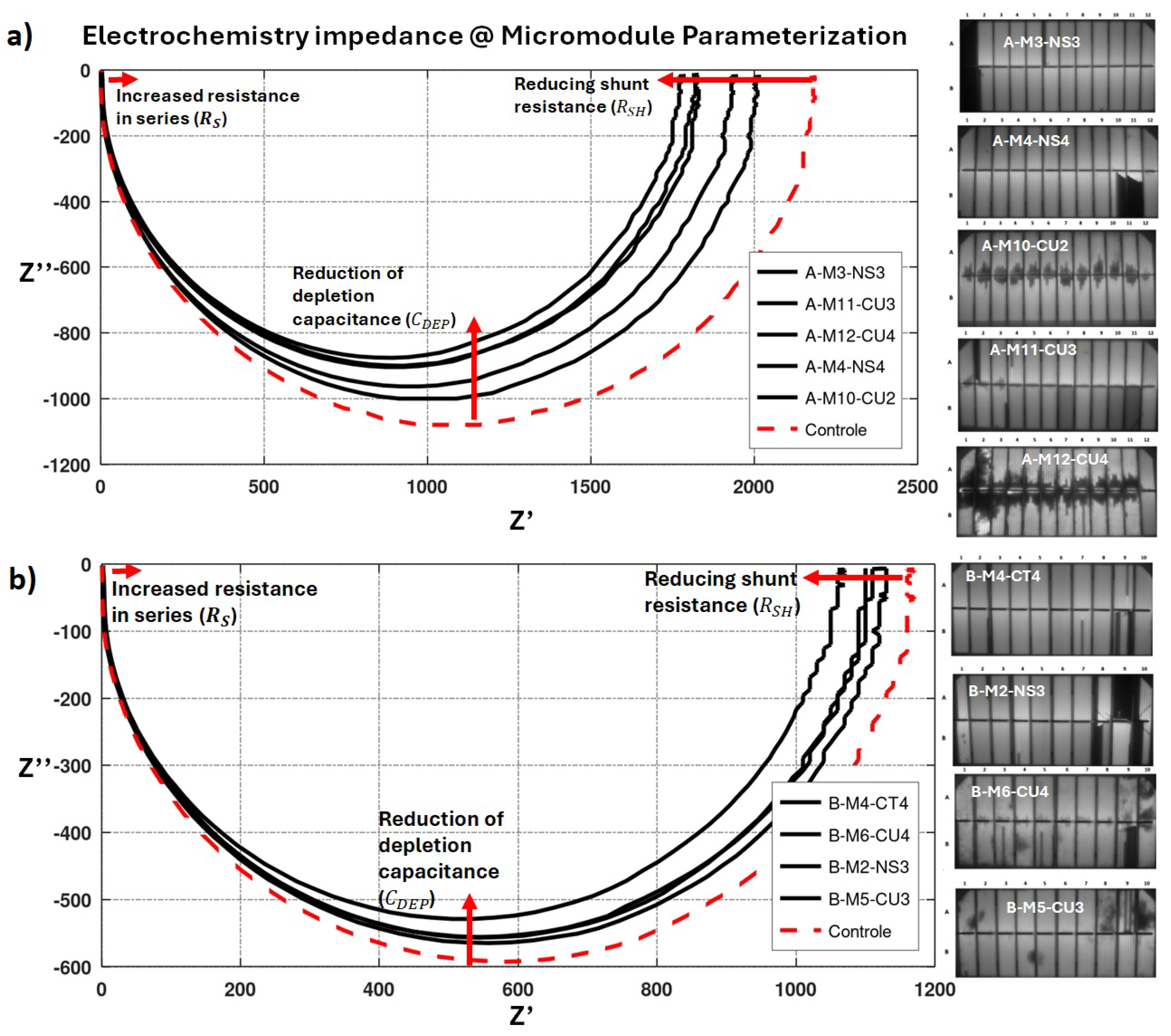
Figure 7.
a) Three-dimensional PCA projection and clustering of tested micromodules b) Magnitude of the most significant variables from the empirical database c) Contributions and direction of each variable’s vectors in 3D PCA and d) Electroluminescence image of the rejected samples and outliers
Figure 7.
a) Three-dimensional PCA projection and clustering of tested micromodules b) Magnitude of the most significant variables from the empirical database c) Contributions and direction of each variable’s vectors in 3D PCA and d) Electroluminescence image of the rejected samples and outliers
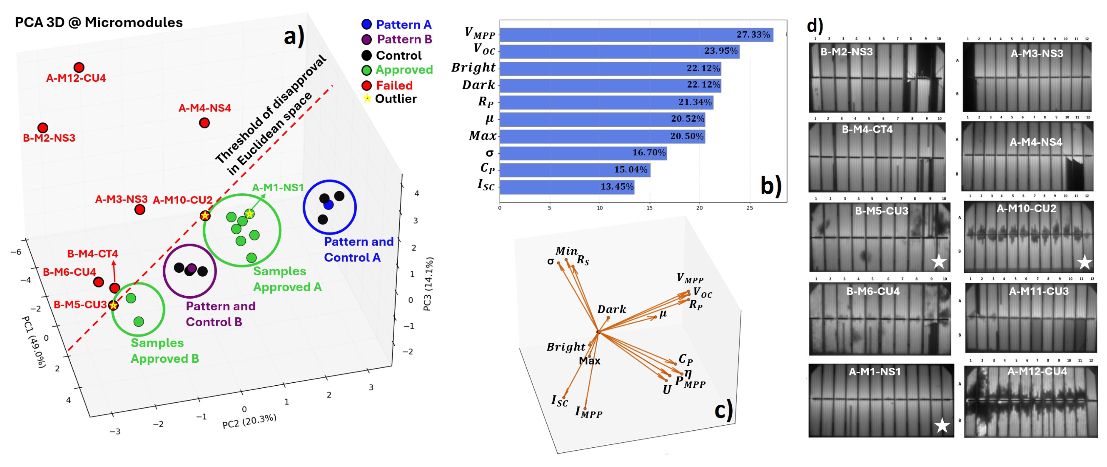
Figure 8.
Correlation heatmap between numeric variables from an empirical database
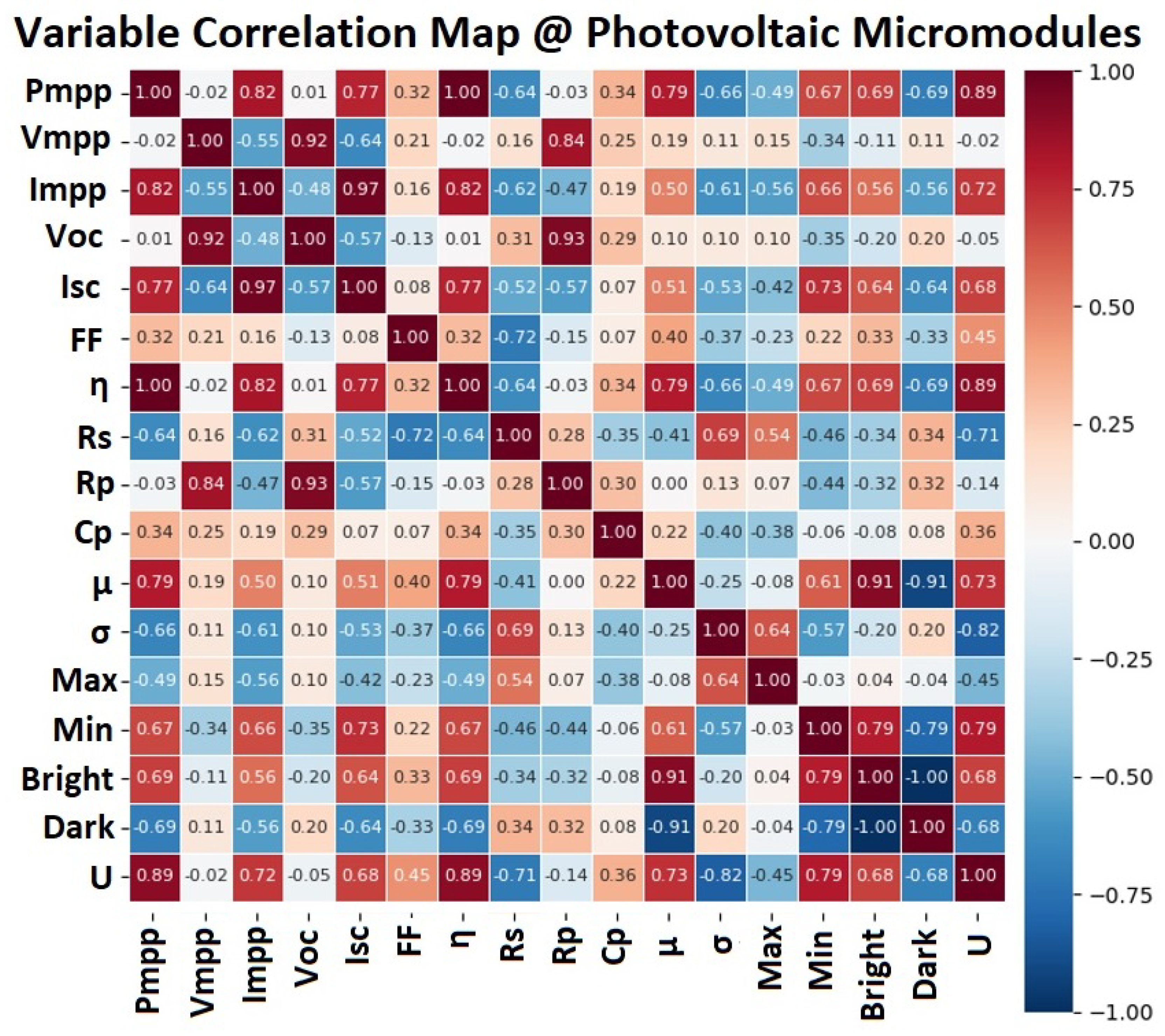
Figure 9.
Classification of samples by the Fuzzy system considering the global degradation criterion of the PV micromodules.
Figure 9.
Classification of samples by the Fuzzy system considering the global degradation criterion of the PV micromodules.
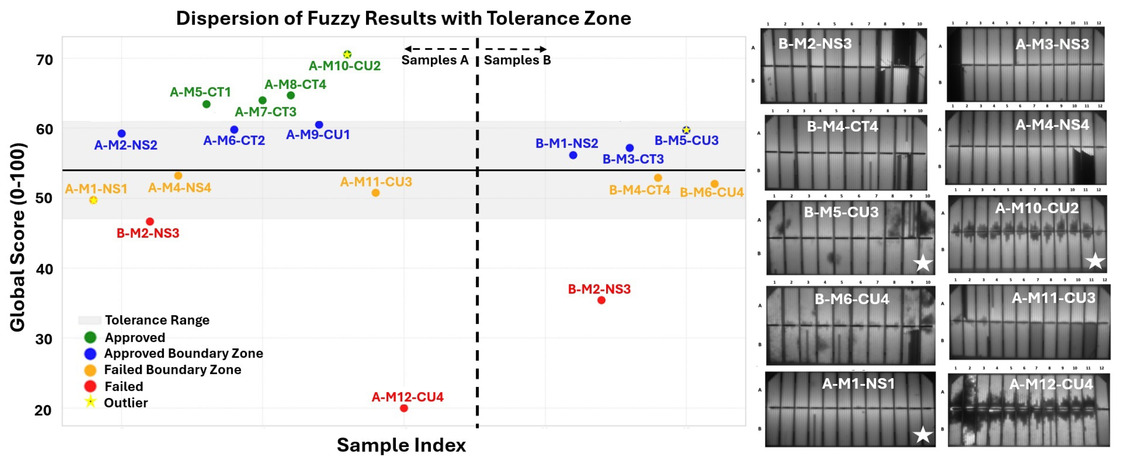
Figure 10.
Degradation analysis results for the Damp Heat test: (a) Weibull fitting; (b) Model residuals; (c) Cumulative failure probability.
Figure 10.
Degradation analysis results for the Damp Heat test: (a) Weibull fitting; (b) Model residuals; (c) Cumulative failure probability.
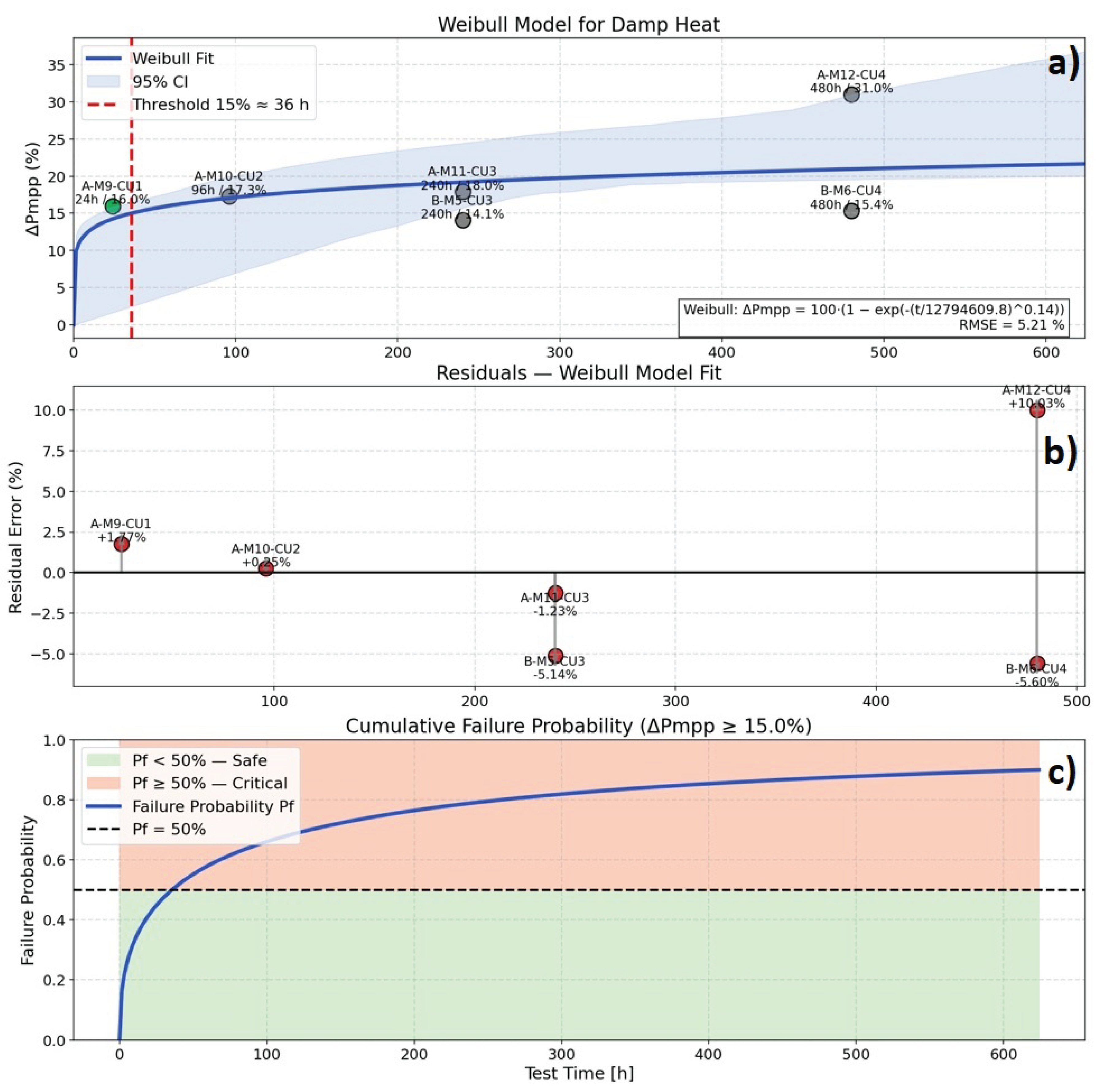
Figure 11.
Degradation analysis results for the Salt Mist test: (a) Weibull fitting; (b) Model residuals; (c) Cumulative failure probability.
Figure 11.
Degradation analysis results for the Salt Mist test: (a) Weibull fitting; (b) Model residuals; (c) Cumulative failure probability.
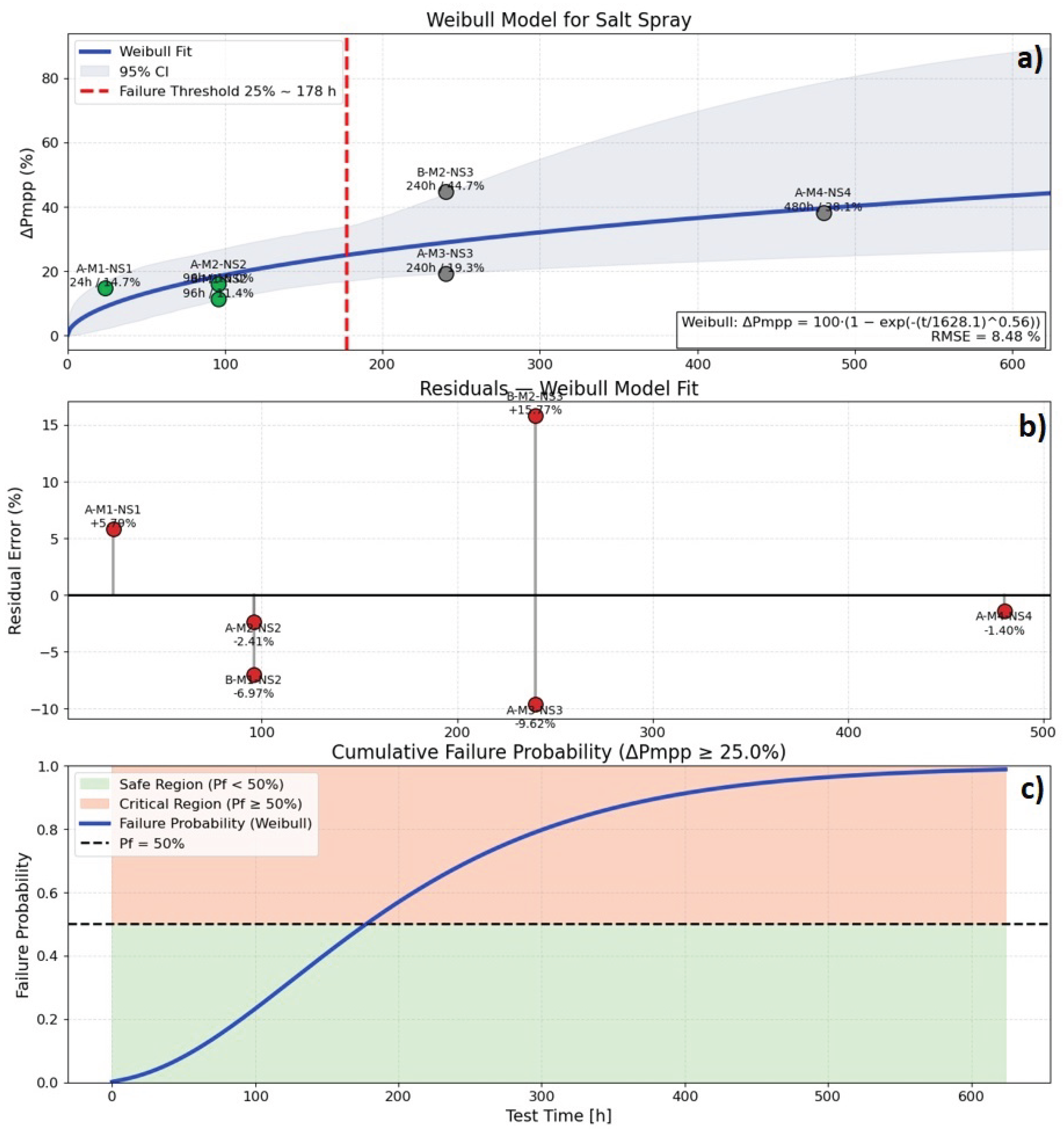
Figure 12.
Degradation analysis results for the Thermal Cycling test: (a) Weibull fitting; (b) Model residuals; (c) Cumulative failure probability.
Figure 12.
Degradation analysis results for the Thermal Cycling test: (a) Weibull fitting; (b) Model residuals; (c) Cumulative failure probability.
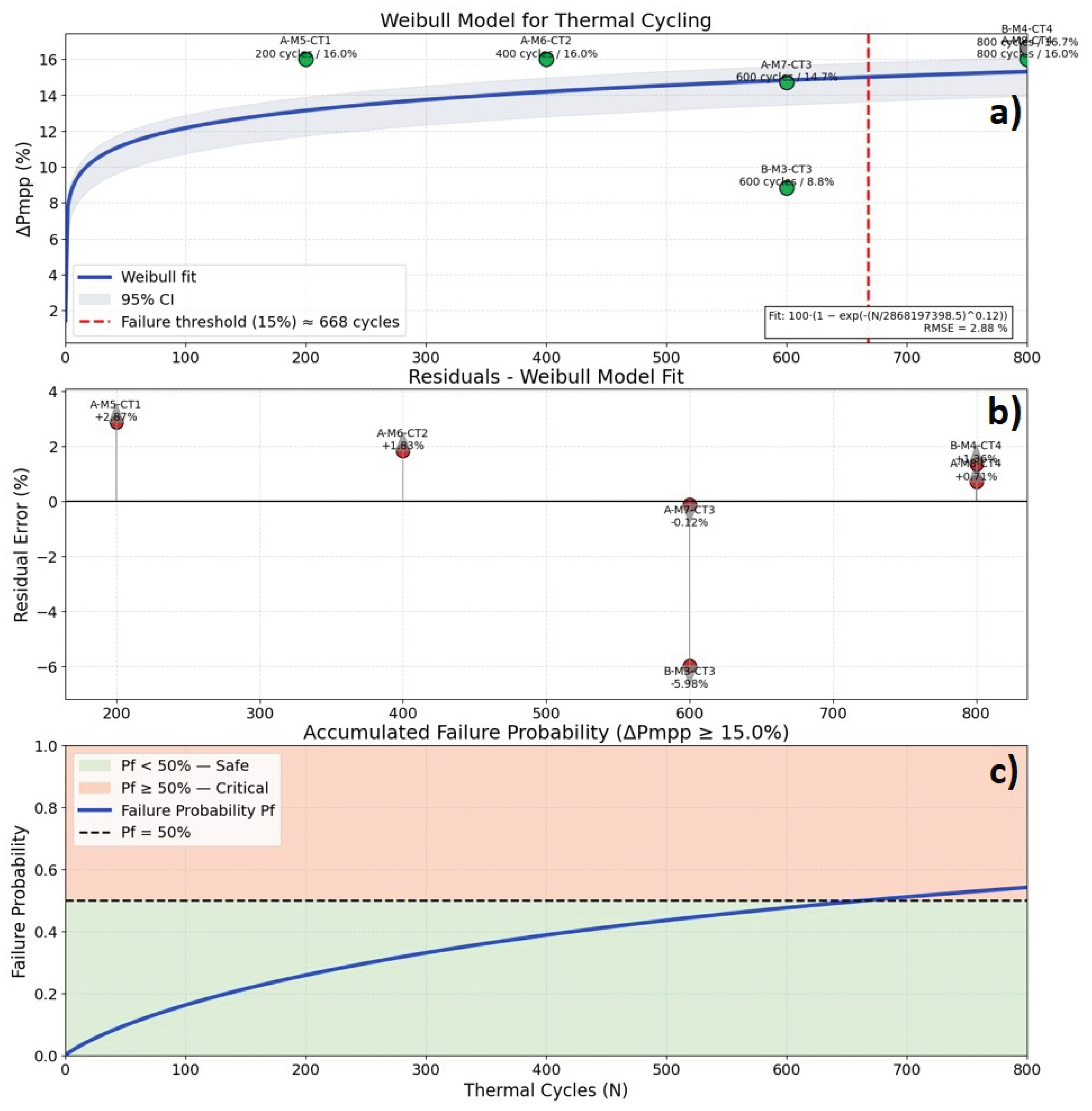

Table 1.
STC electrical parameters provided by the manufacturer for the PV micromodules.
| Family | Pmpp [W] | Vmpp [V] | Impp [A] | Voc [V] | Isc [A] |
|---|---|---|---|---|---|
| A | 1.5 | 6.6 | 0.23 | 7.2 | 0.25 |
| B | 1.5 | 5.7 | 0.27 | 6.0 | 0.30 |
Table 2.
Sample population allocated for characterization.
| Family | No. of | No. of | Total | Control | Test |
|---|---|---|---|---|---|
| cells | busbars | samples | samples | samples | |
| A | 12 | 1 | 15 | 3 | 12 |
| B | 10 | 1 | 9 | 3 | 6 |
Table 3.
Full parametrization of the micromodule population based on I–V, EIS, and EL characterization
Table 3.
Full parametrization of the micromodule population based on I–V, EIS, and EL characterization
| Code | Pulsed I–V Curve | Complex Impedance (EIS) | Electroluminescence EL and Histogram | Result | |||||||||||||
|---|---|---|---|---|---|---|---|---|---|---|---|---|---|---|---|---|---|
| Max | Min | Bright | Dark | U | |||||||||||||
| X | [W] | [V] | [A] | [V] | [A] | [%] | [] | [] | [nF] | [0–255] | [0–255] | [0–255] | [0–255] | [%] | [%] | [%] | X |
| A-C1 | 1.51 | 6.22 | 0.24 | 7.62 | 0.26 | 14.33 | 1.43 | 2484 | 56.8 | 155.20 | 40.48 | 205 | 17 | 55.7 | 44.3 | 0.70 | Control |
| A-C2 | 1.52 | 6.32 | 0.24 | 7.63 | 0.26 | 14.48 | 1.13 | 1956 | 53.1 | 145.70 | 38.06 | 202 | 16 | 54.6 | 45.4 | 0.70 | Control |
| A-C3 | 1.50 | 6.24 | 0.24 | 7.61 | 0.26 | 14.29 | 1.21 | 2143 | 55.8 | 150.30 | 42.45 | 207 | 17 | 58.1 | 41.9 | 0.70 | Control |
| Pattern A | 1.51 | 6.26 | 0.24 | 7.62 | 0.26 | 14.37 | 1.26 | 2194 | 55.2 | 150.40 | 40.33 | 205 | 17 | 56.2 | 43.9 | 0.70 | Media |
| A-M1-NS1 | 1.31 | 5.80 | 0.22 | 7.28 | 0.24 | 12.48 | 1.36 | 2325 | 53.1 | 111.36 | 36.57 | 225 | 22 | 31.90 | 68.10 | 0.67 | Pass |
| A-M2-NS2 | 1.29 | 5.84 | 0.22 | 7.33 | 0.24 | 12.29 | 1.45 | 2189 | 54.2 | 110.32 | 35.84 | 203 | 17 | 30.78 | 69.22 | 0.68 | Pass |
| A-M3-NS3 | 1.24 | 5.38 | 0.23 | 6.71 | 0.25 | 11.81 | 1.41 | 1947 | 39.8 | 107.11 | 45.32 | 197 | 4 | 34.27 | 65.73 | 0.58 | Fail |
| A-M4-NS4 | 0.95 | 6.49 | 0.14 | 7.32 | 0.16 | 9.05 | 1.74 | 1786 | 43.6 | 108.31 | 42.59 | 228 | 9 | 32.77 | 67.23 | 0.61 | Fail |
| A-M5-CT1 | 1.29 | 5.81 | 0.22 | 7.30 | 0.24 | 12.29 | 1.28 | 1963 | 53.7 | 109.63 | 36.73 | 201 | 17 | 30.35 | 69.65 | 0.67 | Pass |
| A-M6-CT2 | 1.29 | 5.82 | 0.22 | 7.31 | 0.24 | 12.29 | 1.42 | 1896 | 54.5 | 112.12 | 35.26 | 184 | 16 | 31.56 | 68.44 | 0.69 | Pass |
| A-M7-CT3 | 1.31 | 5.83 | 0.22 | 7.28 | 0.24 | 12.48 | 1.51 | 1987 | 54.8 | 113.29 | 37.99 | 211 | 18 | 34.15 | 65.85 | 0.66 | Pass |
| A-M8-CT4 | 1.29 | 5.81 | 0.22 | 7.37 | 0.24 | 12.29 | 1.32 | 1893 | 53.6 | 112.91 | 38.17 | 204 | 18 | 33.76 | 66.24 | 0.66 | Pass |
| A-M9-CU1 | 1.29 | 5.87 | 0.22 | 7.33 | 0.24 | 12.29 | 1.47 | 1954 | 54.2 | 107.62 | 39.17 | 215 | 17 | 29.04 | 70.96 | 0.64 | Pass |
| A-M10-CU2 | 1.27 | 5.78 | 0.22 | 7.29 | 0.24 | 12.10 | 1.83 | 1831 | 44.9 | 111.96 | 37.59 | 194 | 17 | 37.79 | 62.21 | 0.66 | Fail |
| A-M11-CU3 | 1.26 | 5.81 | 0.21 | 7.25 | 0.24 | 12.00 | 2.17 | 2017 | 38.8 | 107.31 | 40.10 | 220 | 22 | 31.83 | 68.17 | 0.63 | Fail |
| A-M12-CU4 | 1.06 | 5.44 | 0.19 | 7.29 | 0.24 | 10.10 | 3.17 | 1830 | 39.6 | 111.49 | 50.28 | 247 | 15 | 44.53 | 55.47 | 0.55 | Fail |
| —————– | —– | —– | —– | —– | —– | —– | —– | —– | —– | —– | —– | —– | —– | —– | —– | —– | ———- |
| B-C1 | 1.56 | 5.23 | 0.26 | 6.37 | 0.32 | 14.86 | 0.99 | 1195 | 48.8 | 150.99 | 34.42 | 208 | 43 | 76.77 | 23.23 | 0.77 | Control |
| B-C2 | 1.57 | 5.26 | 0.29 | 6.32 | 0.32 | 14.95 | 1.01 | 1240 | 45.4 | 149.02 | 35.40 | 210 | 43 | 75.98 | 24.02 | 0.76 | Control |
| B-C3 | 1.56 | 5.24 | 0.29 | 6.39 | 0.32 | 14.85 | 0.95 | 1075 | 45.8 | 148.65 | 36.69 | 212 | 40 | 75.03 | 24.97 | 0.75 | Control |
| Pattern B | 1.56 | 5.24 | 0.28 | 6.36 | 0.32 | 14.89 | 0.98 | 1170 | 46.7 | 149.55 | 35.50 | 210 | 42 | 75.90 | 24.10 | 0.80 | Media |
| B-M1-NS2 | 1.36 | 5.02 | 0.27 | 6.08 | 0.29 | 12.95 | 1.01 | 1158 | 48.10 | 112.63 | 35.64 | 180 | 18 | 36.37 | 63.63 | 0.68 | Pass |
| B-M2-NS3 | 0.85 | 5.29 | 0.16 | 6.04 | 0.19 | 8.10 | 1.64 | 1115 | 45.30 | 105.96 | 50.06 | 244 | 9 | 38.14 | 61.86 | 0.53 | Fail |
| B-M3-CT3 | 1.40 | 5.03 | 0.27 | 6.07 | 0.30 | 13.33 | 1.09 | 1142 | 47.40 | 113.84 | 36.34 | 204 | 19 | 37.98 | 62.02 | 0.68 | Pass |
| B-M4-CT4 | 1.28 | 4.71 | 0.27 | 6.04 | 0.30 | 12.19 | 1.10 | 1071 | 45.60 | 113.09 | 37.43 | 203 | 21 | 36.47 | 63.53 | 0.67 | Fail |
| B-M5-CU3 | 1.32 | 4.91 | 0.26 | 6.02 | 0.30 | 12.57 | 1.29 | 1134 | 41.10 | 112.84 | 39.35 | 198 | 19 | 39.23 | 60.77 | 0.65 | Fail |
| B-M6-CU4 | 1.30 | 4.83 | 0.27 | 6.10 | 0.30 | 12.38 | 1.57 | 1103 | 40.90 | 109.72 | 40.06 | 195 | 18 | 40.04 | 59.96 | 0.63 | Fail |
Table 4.
Dominant Physical Meaning of Principal Components
| Component | Dominant physical interpretation |
|---|---|
| PC1 | Optoelectronic variations — , , , , |
| PC2 | Optical variations — , , U, Max, Min, pixel metrics |
| PC3 | Electrical and thermal effects — , , , C |
Table 5.
Centroid coordinates for each class in the PCA space.
| Reference | PC1 | PC2 | PC3 |
|---|---|---|---|
| Standard A | 1.287735 | 2.681381 | 1.266439 |
| Standard B | 5.108676 | -1.122172 | 1.613466 |
| Passed | -0.553305 | 0.747796 | -1.451915 |
| Failed | -2.289544 | -1.440778 | 0.171957 |
Table 6.
Euclidean distances between centroids.
| Reference | Standard A | Standard B | Passed | Failed |
|---|---|---|---|---|
| Standard A | 0.000000 | 5.402503 | 3.810200 | 5.566597 |
| Standard B | 5.402503 | 0.000000 | 6.704578 | 7.544079 |
| Passed | 3.810200 | 6.704578 | 0.000000 | 3.231306 |
| Failed | 5.566597 | 7.544079 | 3.231306 | 0.000000 |
Disclaimer/Publisher’s Note: The statements, opinions and data contained in all publications are solely those of the individual author(s) and contributor(s) and not of MDPI and/or the editor(s). MDPI and/or the editor(s) disclaim responsibility for any injury to people or property resulting from any ideas, methods, instructions or products referred to in the content. |
© 2026 by the authors. Licensee MDPI, Basel, Switzerland. This article is an open access article distributed under the terms and conditions of the Creative Commons Attribution (CC BY) license.
Copyright: This open access article is published under a Creative Commons CC BY 4.0 license, which permit the free download, distribution, and reuse, provided that the author and preprint are cited in any reuse.


