
Submitted:
13 January 2026
Posted:
15 January 2026
You are already at the latest version
Abstract
Considered the possible assembly malfunction in control loop, this paper researches the sliding mode observer(SMO) design for a linearized physical system with environmental disturbances and sensor faults in some constrained conditions on system structure, to set up the fault detection and isolation(FDI) scheme for system in the loop. On one hand, by utilizing the features of fault distribution, the coefficients of fault and disturbance in unobserved subsystem are canceled by state transform under the presumed conditions. Then SMO served in FDI for observable subsystem is constructed, where the convergence of observed error is verified by analysis on Lyapunov functions. On the other hand, for the general situation when fault and disturbance are distributed randomly, the coefficients of fault corresponding to unobserved states are canceled by imposing some similarity transforms on system matrix, such that a reconfigured SMO is designed to counteract and detect the fault in observable subsystem. Furthermore, using inequality transform, the convergence of observed error is shown to be bounded with oscillation, which is proved for the existence of disturbance. Finally, FDI scheme is applied and tested in a fixed-wing airplane system to validate the stability of SMO.
Keywords:
sliding mode observer
; fault isolation
; observable subsystem
; stability transformation
1. Introduction
Fault is appeared possibly in the airplane system due to the aging phenomenon, environmental erosion and assembly damage. Generally, the malfunction in an airplane system is categorized into actuator fault and sensor fault by the different location on the control loop[1,2,3]. Compared with other faults, the sensor is more vulnerable to fault as automation system generally relies on the precise readings of sorts of transducers to acquire state information, thus the detection of sensor faults plays an assisting role in the control loop[4,5,6]. To refine the healthy level of aerial system, the research on the faults detection and isolation(FDI) tends to be crucial that the accessibility of performance index of system is satisfied.
By using some transformation technique on system matrix or maintaining the health conditions by index functions, the FDI research of sensors in the modeled system has been broadly studied, including the sliding mode observer(SMO) which helps cancel faults in model system. By exploiting the structure of uncertainty, the estimation and reconstruction of fault is accomplished by SMO in [7]. [8] addressed the FDI design by regrouping the inputs of system into a suitable structure, with the fault isolation index proposed for FDI design. [9] emphasized the numerical tractability of SMO in the structure and analysis to diagnose faults in system. Moreover, [10,11] researched the fault signal reconstruction by equivalent output error injection based on the detected faults.
Similarly, by joining filter structures in auxiliary system design, the FDI of system is derived and solved by obtaining the state estimate. In [12], a fault detection filter is designed to surmount the residual error of observable subsystem by reconstructing the disturbance inputs. [1] studied the reconstruction of the sensor fault by a simple filter, and transformed the sensor fault into a pseudo-actuator fault to wipe out the fault effect. Besides, [13] designed the parameters of observer for fault detection issue using LMI and line filter techniques such that generated residuals of SMO are robust to uncertainties.
In the application of SMO to physical systems, the FDI with regards to the system characteristics is addressed, especially in improving system performance. For example, [14] proposed a model based FDI scheme and a second-order SMO for rigid manipulators. [15] designed SMO for a modular multi-level converter with half-bridge structure to assume and verify the location of the fault. [5,16] researched the FDI for power electronics and VTOL aircraft, respectively, by the designed performance index, the stability of system is judged. [4,17,18] improved the fault detection, reconstruction and control scheme for a motor system, and SMO & SMC are combined to find the sensorless control strategy. Moreover, [19] applied the fault detection and tolerant control scheme on a flight simulator, with the system trajectories attained along the sliding surface in finite time. However, the influence of pattern in the distribution of system faults has not been thoroughly researched in terms of the stability of SMO.
In this paper, FDI scheme with sensor malfunction and environmental disturbance is discussed by addressing the distribution of the faults in system equations, in the configured system structures. On one hand, under the assumptions on coefficients of fault states, the faulty terms for unobserved subsystem are canceled by state transform, and the SMO is designed to detect and isolate the fault effect at observed port with the stability of observer verified using Lyapunov function. On the other hand, in the general situation of fault distribution, the faults are confined in observed subsystem by similarity transform on system matrix, and SMO is designed to detect the faults in model system by employing inequality transformation. However, the existence of disturbance causes stable oscillation of unobserved state error around zero. Finally, the designed SMO is applied on a fixed-wing airplane system to validate its effect, and show the fitness of proposed SMO to be applied to system in-the-loop with suitable structure. The substantial innovation in this paper can be summarized into the following terms:
- 1.
- As the coefficients of system faults and disturbances meet the counteraction assumption, SMO with compensating terms allocated in output states is designed, such that observed error of system states is convergent, and model system is stable via feedback control;
- 2.
- In the general situation when perturbations are randomly distributed, the similarity transform on system matrices is designed to retain the faults at observed port in the transformed system, and the observed error by SMO is stabilized to the neighborhood of origin, which is verified by Lyapunov function and Inequality transform.
- 3.
- The designed FDI method is applied on an airplane model with different disturbance conditions, and the effect of fault based control is validated in simulation results, including the convergence of observed error, the boundedness of state trajectory under fault and disturbance condition, and the fault detection responses.
Notation.
In this paper, the capitalized bold font denotes a matrix variable, the lowercase denotes a vector, the vector denotes the estimating variable by observer, denotes any matrix norm, denotes real numbered matrices domain with n rows and m columns, denotes the superior bound of function f with respect to variable , denotes a vector where each entry is 1.
2. Preliminary Results
2.1. Airplane Model
Consider the fixed-wing airplane model shown in Figure 1 in lateral motion, the relevant coordinates include ground reference frame , wind reference frame and body reference frame , where directs forward along longitudinal axis, directs to right normal to longitudinal plane, and is obtained via right-hand triad. The lateral motion in consideration is comprised by side-slip angle , rolling angle , rolling velocity p yaw velocity r, as well as washed out filter state of r[20] which is associated to slewing rate. The control input of flight dynamics is constituted by the deflection angles of aileron and rudder, respectively. Then the lateral dynamic equation at zero thrust is formulated in by
where denote the angular velocity transformed from , Y denotes lateral aerodynamic force, denote aerodynamic moment at roll and yaw channel, denote attack angle and track bank angle, are filtered coefficients, and , are coefficients of moment of inertial. Moreover, to analyze the motion at the instant, the small-perturbed linearization is conducted on lateral dynamics on the reference state, say , such that the linearized equation appending disturbance and fault effect is obtained as[20]
where
denote Jacobian matrix at linearized point comprised by aerodynamic derivatives, denotes coefficient matrix of malfunction and disturbance, respectively, denotes the output, and perturbed values
comprise state and control vectors.
2.2. Structural Decomposition of System
Consider the possible environmental disturbance and the malfunction in the sensors, which may cause instability of state response. In order to constrain the effect of malfunctions, appropriate structural transform and analysis are implemented as basic preparation in FDI design. Since coefficient is nonsingular, we can rewrite the linearized equation (1) in the general form as follows
where denotes state vector, denotes control input, and denote sensor malfunction and environmental disturbance on system, respectively, and ,,, denote the coefficient matrix. To facilitate the FDI research of system (2), the following assumption on the magnitude of fault and disturbance is proposed.
Assumption 1.
The perturbation terms caused by malfunction of sensors and environmental disturbance are restricted with , for some real numbers .
To estimate the states of system under the malfunction of sensor, the following observer system is formulated
where is designed to cancel the divergence caused by in (2), denotes output coefficient matrix, and is the feedback coefficient of output error in observer. By subtracting (2) from (3), the equation of observed error is obtained as follows
By designing , the error tends to be stabilized as the perturbations are constricted by compensating term , hence the following assumption is required[21].
Assumption 2.
The system (2) is output observable, namely, forms an observable pair.
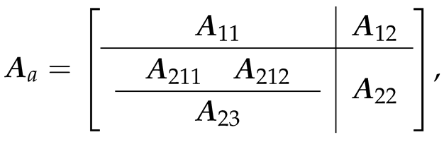
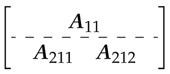
If the state vector is split into , where corresponds to observable part in (2), the system (2) is rewritten as
corresponding to two states. Then state transform is enforced to unobserved part as
where is positive definite, and is suitably configured such that
is a Hurwitz matrix[21], which is important in the convergence of observer system.
Moreover, the controllability of pair is needed to design control law to assure the stability of system. By control law of linear system, the linear feedback control can be derived such that is Hurwitz, and the state is stabilized without the effect of perturbation.
3. Main Results
In this section, the observer to deal with sensor faults is designed via state transformation. Specifically, for perturbations satisfying the proposed assumptions, the state transform (6) is used in the derivation of observer. As for the general case, further coordinate transform is proposed and applied to constitute the observer.
3.1. Fault Isolation by Perturbation Counteracting
Consider the model system (2) which is split into the form of (5), and the coefficient matrix satisfying Assumption 3, the system equation after state transform
is rewritten as
where
To be continued, the following assumption is needed to extend the system transform.
Assumption 3.
The coefficients of malfunction and disturbance can be transformed such that and .
The condition in the assumption corresponds to the situation when perturbations are contained in sensor channels, which can be similarly transformed on the coefficient matrix as fault signals.
By Assumption 3 the perturbations are disappeared in the equation of , and the observer for (7) is designed as
in which denotes output error, and an amending term is added with , where
and
On the other hand, the linear feedback control
is designed such that is Hurwitz. The fault detection and isolation of (7) is discussed as follows.
Theorem 1.
Consider the linear block-partitioned system (7) with perturbations , with SMO proposed in (8) for the FDI scheme of sensors, the observed error is convergent to zero if the following conditions are met
- 1.
- is Hurwitz;
- 2.
- is Hurwitz;
- 3.
- .
Proof.
By subtracting (7) from (8), the equation of observed error is obtained as
by constructing a Lyapunov function , where
is positive definite, we have
where Young’s Inequality[22] is applied in the first inequality with some positive real number , and
as well as Condition 3) is used in the second inequality. By Conditions 1),2), the matrix , is kept negative definite for the appropriately configured eigenvalues on the left hand plane of complex number coordinates, therefore, we have as the Conditions 1)-3) are satisfied. Namely, the observed errors are gradually stabilized in the presence of perturbations.
Besides, for the faulty output channel, the corresponding entry in is switched on its sign, while the entries keep at zero for normal outputs. This means that we can distinguish the fault channel by the response of . Furthermore, by taking control (9) into (8), we have
where
because is convergent, the term is bounded, such that the state by control is solved as
where is used. By the Hurwitz matrix property of , the response is bounded as follows
where , identically, the state of model system are also bounded and stable. □
Remark 1.
In observer system (8) the output feedback is designed as
where , and the Hurwitz stability of and guarantees the stability of overall system matrix since the resulting matrix is in block-partitioned lower triangular form. Furthermore, the state feedback control is taken on the following transformed input matrix
and general form is constructed by firstly extracting the coefficients of eigen-polynomial of as
then by constructing the controllability matrix
and the lower triangular matrix
where is the arbitrary column of such that is full-column rank, the feedback coefficient is configured as follows
Remark 2.
The compensating term in SMO (8) can be directly imposed on fault channel as follows
then
where is nonsingular for some positive definite matrix , and satisfies the relation
such that similar stability criterion can be derived as in (8).
According to the separation principle of control and observer (8), the convergence of state and observed error is obtained, respectively, in a concurrent manner. On the other hand, in a more general situation when the Assumption 3 is not satisfied on malfunction and disturbance , the fault isolation can be accomplished with limited fault distribution via further state transform.
3.2. Fault Isolation with State Transform
For system equation (5), the fault effect appeared in unobserved subsystem is canceled by state transform, such that the fault of sensor is detected and isolated in the observed port. Moreover, the system matrix over unobserved state is adjusted by another state under the detectability condition.
Firstly, by splitting the state into two segments
we assume that the fault phenomena mainly distribute in and the fault-output port satisfies , then is irrelevant to malfunction. Furthermore, the coefficient matrix is full column rank.
The following transformation matrix is proposed
where is designed such that
where is non-singular. By multiplying with , we have
The system matrix multiplied by is partitioned and denoted as follows
 where , , and . In order to stabilize the observed error in unobservable subsystem of , let , the following assumption is applied on system[21].
Assumption 4.
For partitioned system matrix , forms a detectable pair.
Remark 3.
By using Assumption 4, the disturbance and fault are not required in coincident distribution on their coefficients. The amended assumption hints the detectability of in the following equation
which can be met in most situations as
is full column rank.
By Assumption 4, can be stabilized by output feedback. Then another row-transform is imposed on both sides of (5), where the transform matrix is
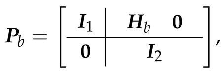 where , and , are identity matrix, and the multiplication of and results in
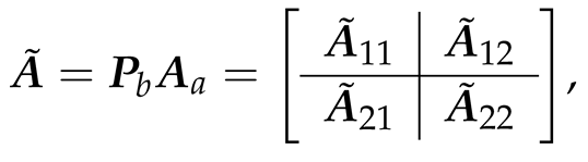 where and
By constructing state transform
system (5) is rewritten as follows
accordingly, the observer is formulated as
in which
where , and denotes coefficient of output feedback. Besides, the feedback control
is designed such that is Hurwitz. The convergence of observed error as well as state is discussed as follows.
Theorem 2.
Consider the model system (5) with malfunction and disturbance , which is transformed to (22) by state transform (21). The sensor fault is detected and isolated by SMO (23) if the following conditions are met:
- 1.
- is Hurwitz matrix;
- 2.
- is Hurwitz matrix;
- 3.
- there exists positive definite matrix such that
- 4.
- the positive real number coefficient in (24) satisfies
Proof.
By subtracting (22) from (23), the equation of observed error is obtained as
namely, is decoupled with , with the solution as follows
since is Hurwitz by condition 1), the first term in (27) is gradually convergent to zero as t approaches to infinity. Therefore, the steady state satisfies the relation
For error , we set up the Lyapunov function with as shown in Condition 3), then its time derivative is
where conditions 2), 3) are used in the first inequality with
satisfied, condition 4) and Young’s Inequality are employed in the third inequality, to counteract the terms of perturbation and the coupled term of and . Consequently, as shown in (28), is bounded to the scale of , then as the eigenvalue of determined by is adjusted such that
the observed error will be stabilized to bounded region
where
as is effective. Namely, the influence of on the system is isolated by observer (23). Specially, by the switch phenomena of , the possible fault element in can be detected.
On the other hand, with the designed control (25), the solution is solved as follows
where
is bounded since and are stable, respectively, as shown in (24),(30). Therefore, as system matrix is configured to be Hurwitz, the observed state is convergent to to be stable, so as to the model state and . □
In the proof, the malfunction is transformed to output channel, and counteracted by designed switch function if specific stability conditions are met. Besides, the disturbance is considered in the stability discussion, which causes observed error evolved in the region around zero.
In summary, the FDI scheme is resolved by SMO according to the structure configuration of system, and both designs are capable of stabilizing the observed error and state trajectory by the Hurwitz stability of feedback coefficient matrix. The structure diagram of the SMO based FDI design is shown in Figure 2, where the transform on the system matrix is sorted in different conditions, whereas the SMO design is concatenated to both situations to detect and isolate fault in the control loop.
4. Simulation Results
In this section, the designed FDI method is tested on the airplane system (1). The aerodynamic parameters of (1) is shown in Table 1, the other parameters are chosen as ,,, , and the initial states are chosen as
Moreover, the perturbations are chosen as
with positive real numbers .
4.1. Perturbations Counteraction
In this case, the transform matrix is chosen as
coefficient matrix of perturbations and faults are
that meet the Assumption 3. The observer is constructed as in (8) where observer gain and the coefficient of feedback control designed as per (12),(13) are given as follows
moreover, fault estimator is constructed as
in which
with as discussed in (15). In Figure 3 the plot of fault estimator show some obvious oscillations after , and the two components nearly coincide with each other. Then in Figure 3, it is shown that observed errors are bounded in range . Moreover, in order to indicate the ability of fault detection of (8), the fault is posed at the fourth row of and , and the responses of compensating term are shown in Figure 4, where the elements are zero, and major oscillation lies at . Namely, the fault is detected by the entries of .
4.2. State Transform
In the general case when the cancellation of and are disabled, the coordinate transform as discussed in subSection 3.2 is used to place the faults in the sensor channels except the detected counter-part shown in (17). The fault coefficient is
the transform matrix in (21) are computed as
and the coefficient matrix in (24) is calculated to be
The responses of states and the estimate states are shown in Figure 5Figure 6, where all the states are coincided with the estimate. The angle variables are confined within , and the filtered angular velocity is considerably constrained on magnitude compared with r. In Figure 7, the observed errors are stabilized within , and the responses of compensating term shows that main overshoots are distributed at terms in response to fault variation, as shown in Figure 7. This demonstrates that the proposed fault estimator is able to detect and isolate the faults via SMO and coordinate transform.
Furthermore, the distributions of in profiles (10) and (26), say , , are compared and shown by box plot in Figure 8. As shown in plot, the mean of coincides with 0, and the whiskers spread to ; meanwhile, the mean of departs from 0, with approximating magnitude , and the magnitudes whiskers reach to are ranged in . Besides, the statistics of and are listed in Table 2, which is congruent to the trend in box plot. Namely, we can find that the observed precision by matrix transform in (23) is more advanced than (8) by state organization. By the FDI scheme with regards to specific system configuration, the application in reliable control of physical systems is possibly pushed forward.
5. Conclusion
In this paper, the FDI scheme with sensor malfunctions and environmental disturbances is researched to detect the location of malfunctions in sensor and guarantee the convergence of observer by isolating the faults. According to the distribution of faults, on one hand, the coefficients of faults and disturbances in unobserved subsystem are canceled by state transform, then the stability of the observed error is discussed with regards to the proposed sliding surface. Based on the state estimate provided by SMO, the stability of model system is obtained by feedback control. On the other hand, for the more general distribution of sensor faults and disturbances, the faults are retained at observed subsystem by similarity transform of system matrix, together with SMO to detect and isolate the faults. By using Lyapunov function and inequality transform, the boundedness of system states is proved, with the induced oscillation by disturbances. Finally, the researched methods are applied on a fixed-wing airplane system to validate the theoretical derivation. In the future, the performance of SMO including response time and observed precision will be further evaluated and compared.
Author Contributions
Conceptualization, Xiaoping Chen and Xiaobo Ma; methodology, Bowen Su; validation, Yuehong Dai; formal analysis, Bowen Su; writing—original draft preparation, Bowen Su; project administration, Xiaobo Ma; funding acquisition, Yuehong Dai. All authors have read and agreed to the published version of the manuscript.
Funding
This research was funded by Advanced Fund of Equipment Development Department of Central Military Commission, CN on grant number 30103090201 and Pioneer Fund of System & Artificial Intelligence Key Laboratory, Sichuan on grant number SSAI202503.
Data Availability Statement
The original data presented in the study are openly available in [Fault-diagnosis-program] at [https://github.com/BowenSususu/Fault-diagnosis-program/tree/main].
Acknowledgments
During the preparation of this manuscript/study, the author(s) used [MATLAB] for the purposes of [data analysis, model solving].
Conflicts of Interest
The authors declare no conflicts of interest.
References
- Yan, X.G.; Edwards, C. Sensor fault detection and isolation for nonlinear systems based on a sliding mode observer. International Journal of Adaptive Control and Signal Processing 2007, 21, 657–673. [Google Scholar] [CrossRef]
- Falcón, R.; Rios, H.; Dzul, A. A robust fault diagnosis for quad-rotors: A sliding-mode observer approach. IEEE/ASME Transactions on Mechatronics 2022, 27, 4487–4496. [Google Scholar] [CrossRef]
- Isermann, R. Fault-diagnosis systems: an introduction from fault detection to fault tolerance; Springer Science & Business Media: Berlin, 2005. [Google Scholar]
- Mekki, H.; Benzineb, O.; Boukhetala, D.; Tadjine, M.; Benbouzid, M. Sliding mode based fault detection, reconstruction and fault tolerant control scheme for motor systems. ISA Transactions 2015, 57, 340–351. [Google Scholar] [CrossRef] [PubMed]
- Li, J.; Pan, K.; Su, Q. Sensor fault detection and estimation for switched power electronics systems based on sliding mode observer. Applied Mathematics and Computation 2019, 353, 282–294. [Google Scholar] [CrossRef]
- Shahzad, E.; Khan, A.U.; Iqbal, M.; Saeed, A.; Hafeez, G.; Waseem, A.; Albogamy, F.R.; Ullah, Z. Sensor fault-tolerant control of microgrid using robust sliding-mode observer. Sensors 2022, 22, 2524. [Google Scholar] [CrossRef] [PubMed]
- Yan, X.G.; Edwards, C. Robust decentralized actuator fault detection and estimation for large-scale systems using a sliding mode observer. International Journal of Control 2008, 81, 591–606. [Google Scholar] [CrossRef]
- Chen, W.; Saif, M. A sliding mode observer-based strategy for fault detection, isolation, and estimation in a class of Lipschitz nonlinear systems. International Journal of Systems Science 2007, 38, 943–955. [Google Scholar] [CrossRef]
- Edwards, C.; Spurgeon, S.K. On the development of discontinuous observers. International Journal of Control 1994, 59, 1211–1229. [Google Scholar] [CrossRef]
- Edwards, C.; Spurgeon, S.K.; Patton, R.J. Sliding mode observers for fault detection and isolation. Automatica 2000, 36, 541–553. [Google Scholar] [CrossRef]
- Yan, X.; Edwards, C. Robust sliding mode observer-based actuator fault detection and isolation for a class of nonlinear systems. International Journal of Systems Science 2008, 39, 349–359. [Google Scholar] [CrossRef]
- Floquet, T.; Barbot, J.P.; Perruquetti, W.; Djemai, M. On the robust fault detection via a sliding mode disturbance observer. International Journal of Control 2004, 77, 622–629. [Google Scholar] [CrossRef]
- Zhang, K.; Jiang, B.; Yan, X.G.; Mao, Z. Sliding mode observer based incipient sensor fault detection with application to high-speed railway traction device. ISA transactions 2016, 63, 49–59. [Google Scholar] [CrossRef] [PubMed]
- Brambilla, D.; Capisani, L.M.; Ferrara, A.; Pisu, P. Fault Detection for Robot Manipulators via Second-Order Sliding Modes. IEEE Transactions on Industrial Electronics 2008, 55, 3954–3963. [Google Scholar] [CrossRef]
- Shao, S.; Wheeler, P.W.; Clare, J.C.; Watson, A.J. Open-circuit fault detection and isolation for modular multilevel converter based on sliding mode observer. In Proceedings of the 2013 15th European Conference on Power Electronics and Applications (EPE), 2013; pp. 1–9. [Google Scholar]
- Tan, C.P.; Edwards, C. Sliding mode observers for robust detection and reconstruction of actuator and sensor faults. International Journal of Robust and Nonlinear Control: IFAC-Affiliated Journal 2003, 13, 443–463. [Google Scholar] [CrossRef]
- Zuo, Y.; Lai, C.; Iyer, K.L.V. A review of sliding mode observer based sensorless control methods for PMSM drive. IEEE Transactions on Power Electronics 2023, 38, 11352–11367. [Google Scholar] [CrossRef]
- Ding, H.; Zou, X.; Li, J. Sensorless control strategy of permanent magnet synchronous motor based on fuzzy sliding mode observer. IEEE Access 2022, 10, 36743–36752. [Google Scholar] [CrossRef]
- Edwards, C.; Alwi, H.; Tan, C.P. Sliding mode methods for fault detection and fault tolerant control with application to aerospace systems. International Journal of Applied Mathematics and Computor Science 2012, 22, 109–124. [Google Scholar] [CrossRef]
- Roger, P. Flight control systems: practical issues in design and implementation; Iet: London, UK, 2000. [Google Scholar]
- Callier, F.M.; Desoer, C.A. Linear system theory; Springer Science & Business Media: Berlin, Germany, 2012. [Google Scholar]
- Yin, J.; Khoo, S. Continuous finite-time state feedback stabilizers for some nonlinear stochastic systems. International Journal of Robust and Nonlinear Control 2015, 25, 1581–1600. [Google Scholar] [CrossRef]
Figure 1.
Plot of a fixed-wing airplane in coordinates frame
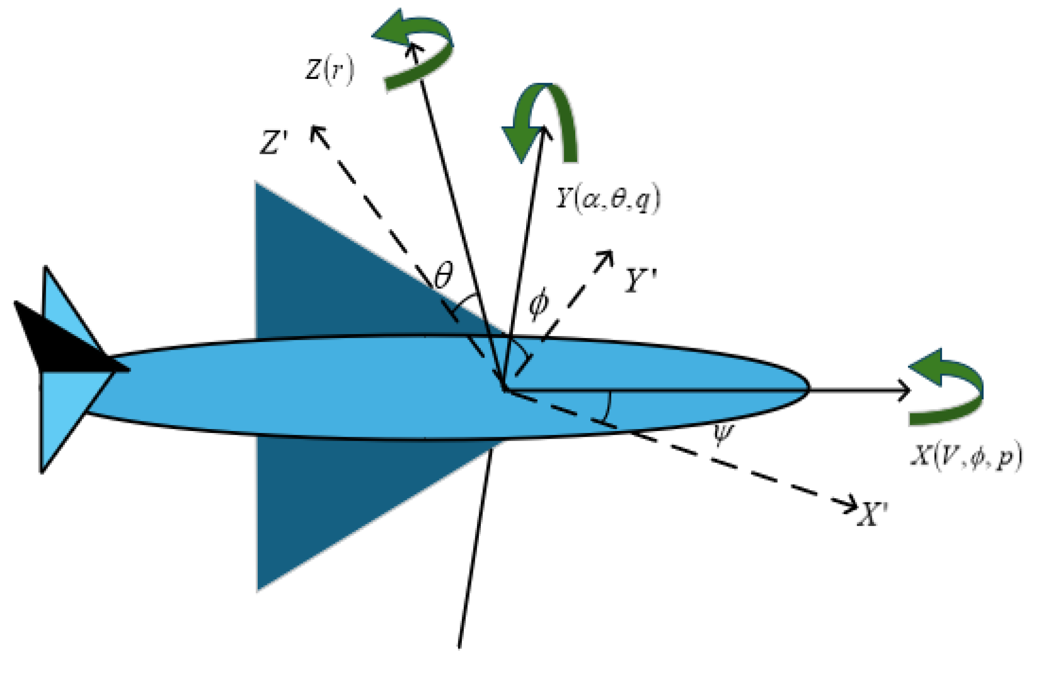
Figure 2.
Structural diagram showing the links on SMO design for FDI scenario in the control loop.
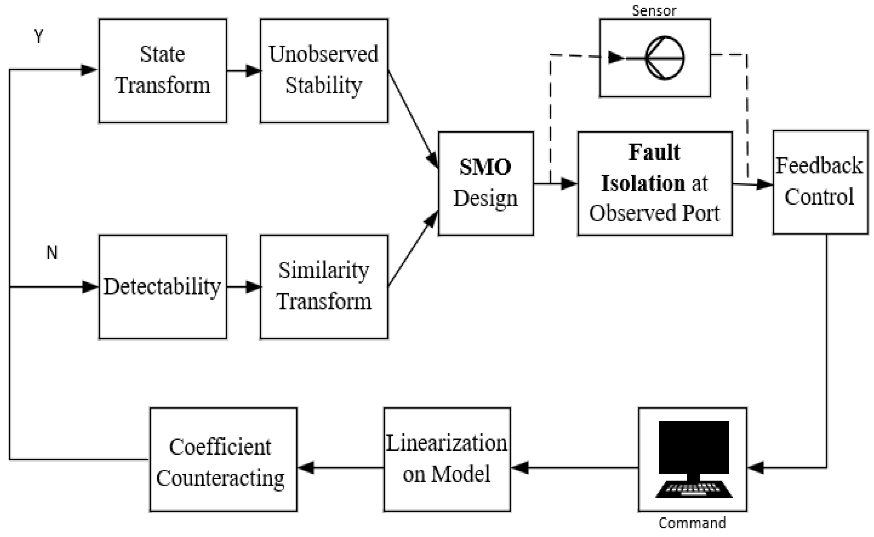
Figure 3.
Responses of fault detection with counteraction by observer (8). (Figure 3): plot of compensating variable ; (Figure 3): plot of observed error .
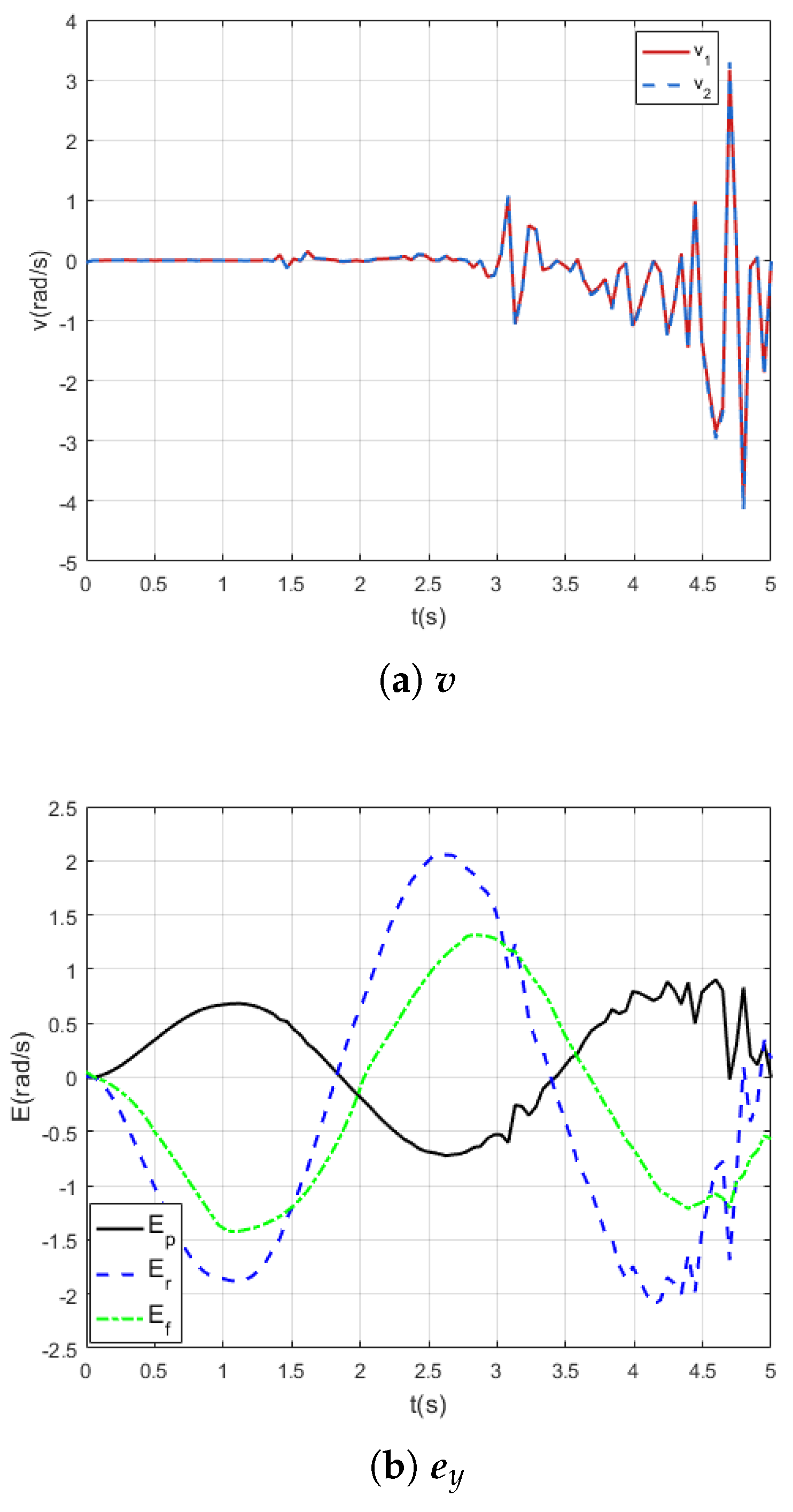
Figure 4.
Responses of fault detection signals in distinguishing certain fault.
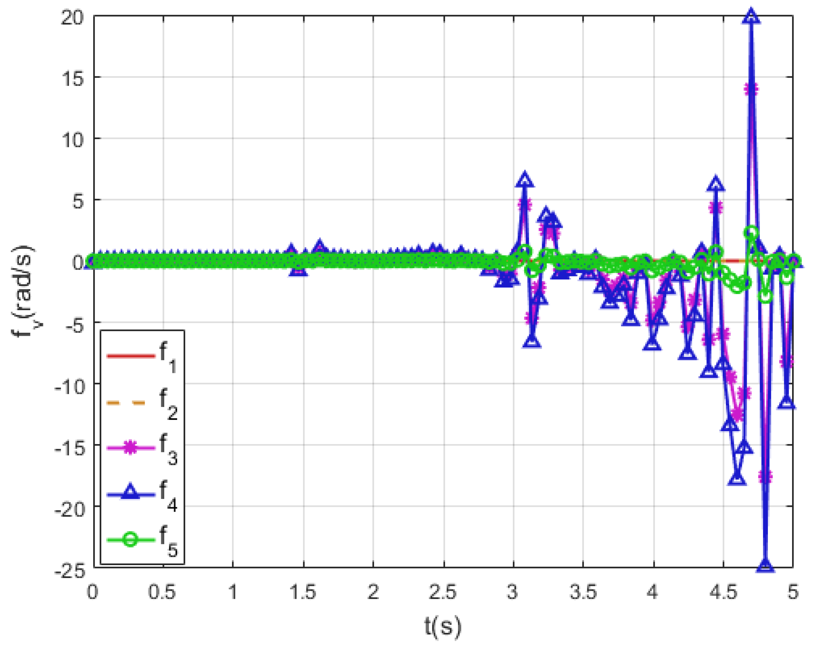
Figure 5.
Responses of states and the estimate with state-transform fault detection by observer (23). (Figure 5): plot of ; (Figure 5): plot of .
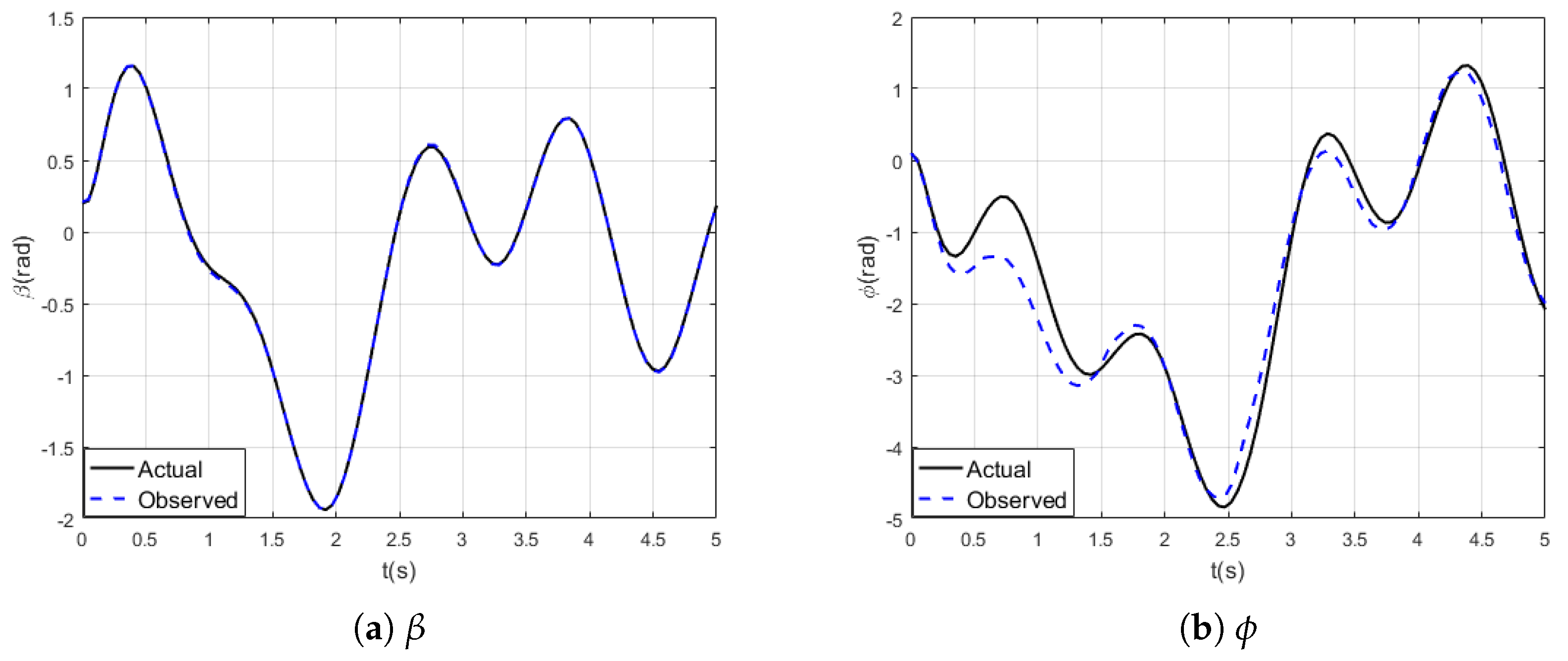
Figure 6.
Responses of states and the estimate with state-transform fault detection by observer (23). (Figure 6): plot of r; (Figure 6): plot of .
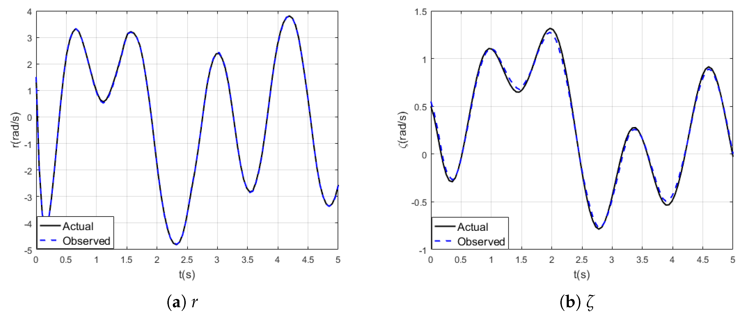
Figure 7.
Responses of fault detection with state transform by observer (23). (Figure 7): plot of observed errors ; (Figure 7): plot of indicating function .
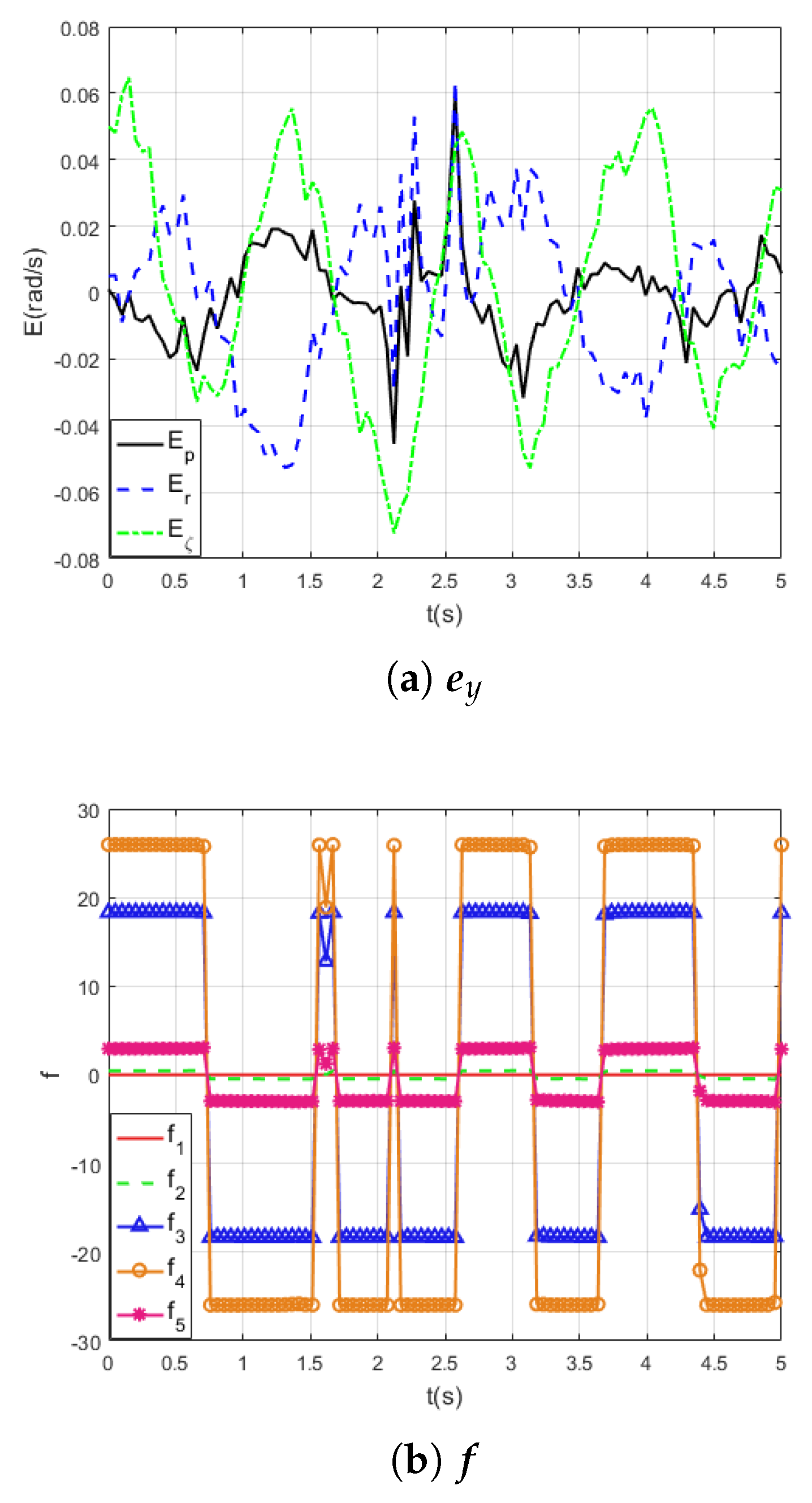
Figure 8.
Box plot of output error in two profiles. The upper plot corresponds to error in (26), and the lower plot corresponds to error in (10).
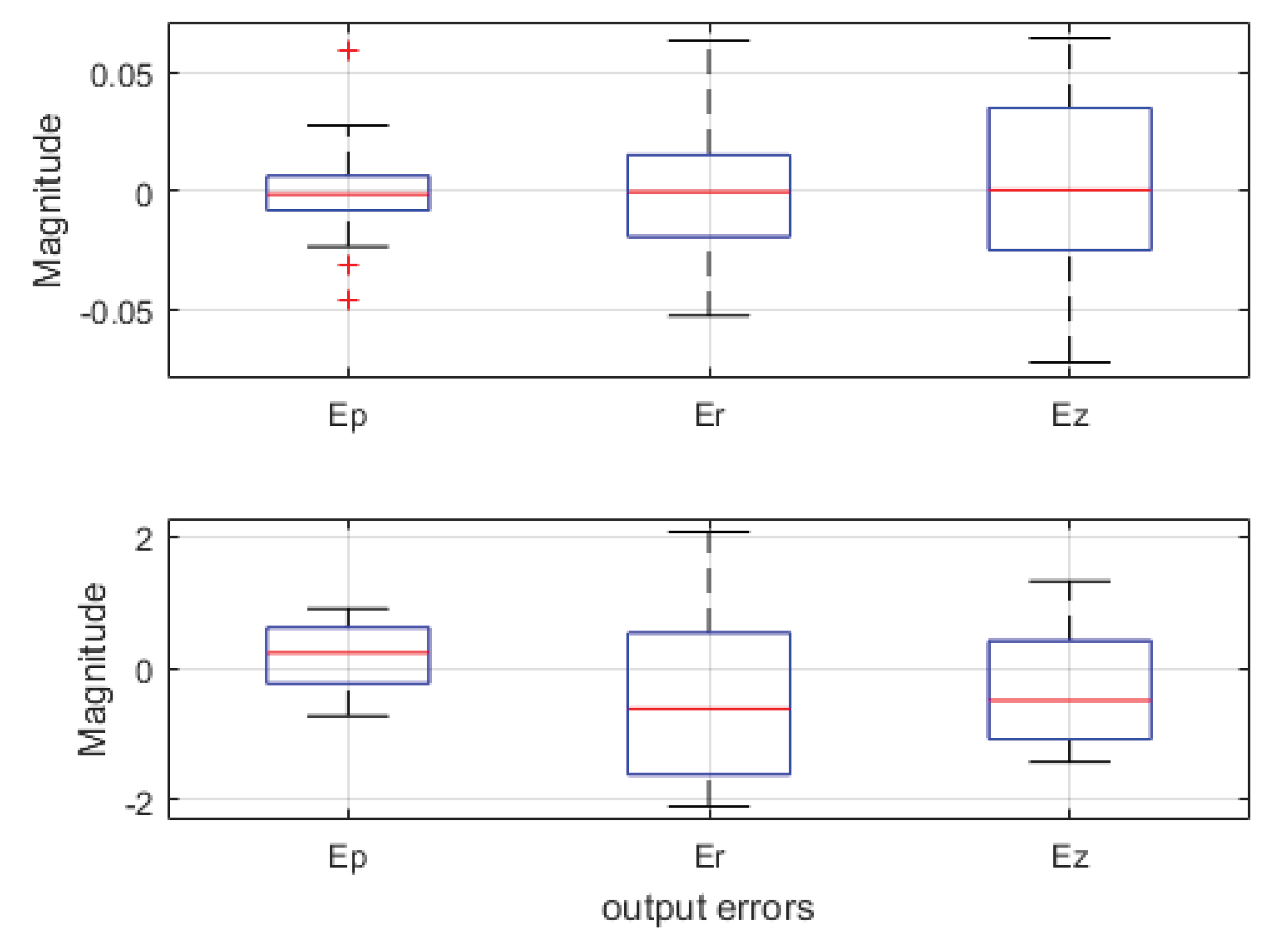

Table 1.
Aerodynamic parameters used in equation (1)
Table 1.
Aerodynamic parameters used in equation (1)
| 0.3 | 2.3 | ||||
|---|---|---|---|---|---|
| 1.2 | |||||
| 2.24 | |||||
| -0.4 | 2.59 | ||||
| 0.5 | 2.67 |
Table 2.
The statistics of in two designed profiles of SMO
| mean | 0.1722 | -0.3769 | -0.2750 | -0.0007 | -0.0023 | 0.0024 |
| max | 0.9014 | 2.0628 | 1.3159 | 0.0595 | 0.0635 | 0.0647 |
| min | -0.7230 | -2.0954 | -1.4219 | -0.0454 | -0.0526 | -0.0723 |
Disclaimer/Publisher’s Note: The statements, opinions and data contained in all publications are solely those of the individual author(s) and contributor(s) and not of MDPI and/or the editor(s). MDPI and/or the editor(s) disclaim responsibility for any injury to people or property resulting from any ideas, methods, instructions or products referred to in the content. |
© 2026 by the authors. Licensee MDPI, Basel, Switzerland. This article is an open access article distributed under the terms and conditions of the Creative Commons Attribution (CC BY) license (http://creativecommons.org/licenses/by/4.0/).
Copyright: This open access article is published under a Creative Commons CC BY 4.0 license, which permit the free download, distribution, and reuse, provided that the author and preprint are cited in any reuse.


