
Submitted:
13 January 2026
Posted:
15 January 2026
You are already at the latest version
Abstract
The Normalized Difference Vegetation Index (NDVI) derived from polar-orbiting satellites is widely used for vegetation monitoring; however, its temporal continuity is often limited by cloud contamination and fixed revisit cycles. This study investigates the feasibility of using geostationary satellite observations to support NDVI gap filling applications and continuous regional monitoring. Geostationary Ocean Color Imager II (GOCI-II) data were used as input, while Sentinel-2 Multispectral Instrument (MSI) NDVI served as the primary reference dataset. Landsat Operational Land Imager NDVI was additionally employed for independent cross-sensor comparison. A data-driven transformation framework was developed and applied to convert GOCI-II NDVI into MSI-equivalent NDVI while maintaining physically interpretable NDVI values. The transformed NDVI was evaluated through spatial comparisons and pixel-level statistical metrics, including correlation coefficient, mean absolute error, root mean square error, and structural similarity index measure. The results indicate that NDVI transformed from geostationary observations can capture broad spatial patterns and relative variability observed in MSI NDVI, particularly at the field scale. At the same time, reduced contrast and NDVI underestimation are observed, mainly due to spatial resolution differences and sub-pixel heterogeneity. This study emphasizes the potential role of geostationary satellite data as a complementary source for polar-orbiting NDVI products. The findings suggest that integrating geostationary and polar-orbiting satellite observations may contribute to improving NDVI continuity and supporting sustained vegetation monitoring over fixed regions where high temporal resolution is required.
Keywords:
NDVI gap filling
; geostationary satellite observations
; polar-orbiting satellite
; reginal vegetation monitoring
; cross-orbit data fusion
1. Introduction
The Normalized Difference Vegetation Index (NDVI) is a widely used indicator in remote sensing for quantifying vegetation condition and has been extensively applied in agricultural monitoring, crop yield estimation, and vegetation change detection[1,2,3]. NDVI analysis based on optical satellite imagery is particularly effective for capturing periodic vegetation dynamics at regional scales[4], and freely available medium-resolution polar-orbiting satellites such as Sentinel-2 and Landsat are commonly utilized for this purpose. However, polar-orbiting satellite–based monitoring inherently suffers from data gaps caused by cloud contamination, as observations are acquired at fixed revisit intervals[5,6]. These cloud-induced missing pixels often degrade the temporal continuity of NDVI time series, making continuous monitoring of a fixed region difficult and consequently reducing the reliability of time-series–based vegetation analysis and change detection.
To address these limitations, previous studies have proposed various gap-handling strategies, including temporal interpolation, multi-temporal data fusion, and cloud-gap reconstruction using synthetic aperture radar observations[7,8,9,10,11,12,13,14,15]. While these approaches can partially mitigate missing data, they remain fundamentally constrained by the revisit cycles of polar-orbiting satellites and therefore cannot fully support continuous or quasi-real-time monitoring of a fixed area. From this perspective, geostationary satellites, which continuously observe the same region at short temporal intervals, offer a promising complementary solution to overcome the inherent limitations of polar-orbiting satellite observations.
Geostationary satellites acquire repeated observations of the same area within short time intervals, and because cloud positions change over time, pixels obscured by clouds at one observation time may be visible at another. In East Asia, the GEO-KOMPSAT-2B (GK-2B) satellite, launched in 2020 and carrying the Geostationary Ocean Color Imager II (GOCI-II), provides multispectral observations in the visible and near-infrared bands over regions including China, the Korean Peninsula, and Japan. GOCI-II acquires imagery at hourly intervals, enabling the capture of dense temporal observations that are difficult to obtain using polar-orbiting sensors alone[16]. Despite this advantage, the integration of GOCI-II with polar-orbiting satellite data for terrestrial vegetation monitoring has been limited, primarily due to its relatively coarse spatial resolution of approximately 250 m. This resolution differs substantially from that of Sentinel-2 Multispectral Instrument (MSI) (10 m) and Landsat Operational Land Imager (OLI) (30 m), imposing significant constraints on direct comparison and gap filling applications.
Recent advances in deep learning–based spatial downscaling techniques have demonstrated strong potential for transforming coarse-resolution satellite imagery into higher-resolution products. Convolutional neural network–based models, including U-Net architectures, have shown effective performance in enhancing spatial detail while preserving large-scale patterns[17,18]. However, most existing studies focus primarily on improving the performance of downscaling algorithms themselves, with limited attention given to the practical role of geostationary satellites as reference monitoring data for continuous NDVI observation. In particular, the potential of high-resolution geostationary NDVI products as auxiliary inputs for polar-orbiting satellite NDVI gap filling has not been sufficiently explored.
This study aims to address this research gap by evaluating the feasibility and effectiveness of high-resolution GOCI-II NDVI for continuous vegetation monitoring over a fixed region. The study area is defined as agricultural regions in Anhui Province, China, where frequent cloud cover poses significant challenges for optical remote sensing–based vegetation monitoring. MSI NDVI is employed as the primary polar-orbiting satellite dataset, while GOCI-II NDVI is used as the geostationary auxiliary dataset. Rather than focusing on gap filling algorithms themselves, this study concentrates on assessing the validity of high-resolution GOCI-II NDVI as a potential input for future gap reconstruction.
2. Data and Study Area
In this study, GK-2B GOCI-II data and Sentinel-2A/B MSI data were used to train and test the AI model. Independent validation was performed using Landsat-8/9 OLI data.
GOCI-II data onboard the GK-2B satellite were used as the input data for model generation. The GK-2B satellite was launched on 18 February 2020 (UTC), and routine operations of the GOCI-II sensor began in October 2020. GOCI-II observes 12 spectral bands spanning the visible to near-infrared wavelengths from 380 to 865 nm, with an hourly temporal resolution and a spatial resolution of 250 m. In this study, Level-2 (L2) Land Surface Reflectance (SRL) data from Slot 10 of the Local Area coverage around the Korean Peninsula were used. NDVI was derived from Band 8 at 660 nm and Band 12 at 865 nm. GOCI-II L2 SRL data are provided by the National Ocean Satellite Center under the Korea Hydrographic and Oceanographic Agency and are publicly available through the official data portal, with data accessible from October 2020 to the present.
Sentinel-2 MSI data were used as the target output for model generation. Sentinel-2A was launched on 23 June 2015 (UTC), and Sentinel-2B was launched on 7 March 2017 (UTC). Data from both satellites were jointly used in this study. Each satellite has a nominal revisit cycle of 10 days, and the combined use of Sentinel-2A and Sentinel-2B enables a revisit interval of approximately 5 days. The MSI sensor consists of 13 spectral bands covering the visible to shortwave infrared wavelengths from 443 to 2190 nm, with spatial resolutions of 10, 20, and 60 m depending on the band. In this study, Level-2A (L2A) bottom-of-atmosphere (BOA) surface reflectance (SR) data from the T51SLC tile were used. NDVI was derived from Band 4 at 665 nm and Band 8 at 842 nm, both with a spatial resolution of 10 m. Sentinel-2 MSI L2A BOA SR data are publicly available through the Copernicus Data Space Ecosystem operated by the European Space Agency on behalf of the European Union’s Copernicus Programme, with data accessible from December 2018 to the present.
Landsat OLI data were used as additional independent datasets for comparative validation of the model results. Landsat-8 was launched on 11 February 2013 (UTC), and Landsat-9 was launched on 27 September 2021 (UTC). Observations from both satellites were jointly used for the analysis. Each satellite has a nominal revisit cycle of 16 days, and the combined use of Landsat-8 and Landsat-9 enables an effective revisit interval of approximately 8 days. The OLI sensor acquires 11 spectral bands covering wavelengths from 443 to 1200 nm, with spatial resolutions of 15, 30, and 100 m depending on the band. In this study, United States Geological Survey (USGS) Landsat Collection 2 L2 SR Science Products were used. NDVI was derived from Band 4 at 655 nm and Band 5 at 865 nm, both with a spatial resolution of 30 m. Landsat OLI SR data are publicly available through the USGS EarthExplorer platform, with data accessible from December 2020 to the present.
Table 1 summarizes the spectral bands, central wavelengths, and spatial resolutions of the satellite sensors used for NDVI computation in this study. Sentinel-2 refers to Sentinel-2A/B, and Landsat refers to Landsat-8/9.
The NDVI data used in this study were calculated from the sensor-specific observations described above. NDVI was derived using a combination of a red band in the visible wavelength range around 600 nm and a near-infrared band around 800 nm. The NDVI was computed using the following equation [19]:
where denotes the surface reflectance provided by each sensor, and and represent the near-infrared and red spectral bands, respectively. Table 2 summarizes representative NDVI values associated with major land cover categories [20], as commonly reported in previous remote sensing studies. Negative or near-zero NDVI values are typically linked to water bodies, while low positive values correspond to bare soil or sparsely vegetated surfaces. As NDVI increases, vegetation cover becomes progressively denser, with higher values indicating moderate to dense vegetation conditions. These NDVI ranges are not intended as strict classification thresholds, but rather as indicative reference values to support the interpretation of NDVI distributions in this study.
The study area was selected over part of Anhui Province, a major agricultural region in central China characterized by extensive cropland coverage and pronounced seasonal vegetation dynamics. These characteristics provide favorable conditions for analyzing NDVI variability and for comparing geostationary satellite–derived NDVI with polar-orbiting satellite observations within a consistent observational domain. Figure 1 illustrates the geographical location of the study area.
3. Methods
This study employed a data-driven NDVI transformation framework to convert GOCI-II NDVI into MSI–equivalent NDVI for evaluating geostationary satellite-based approaches for NDVI gap filling purposes. The framework was designed to address the spatial inconsistencies between geostationary and polar-orbiting satellite observations while preserving physically interpretable NDVI values. Figure 2 illustrates the overall workflow employed in this study, including NDVI normalization, transformation of GOCI-II NDVI into MSI–equivalent NDVI, and comparative evaluation among the transformed NDVI, reference MSI NDVI, and independent OLI NDVI.
The datasets used in this study cover the period from January 2023 to December 2025. Paired NDVI cases were selected when the observation times of GOCI-II and MSI overlapped, and scenes with cloud coverage of 15% or less were retained for NDVI transformation. Cloud coverage was estimated based on the quality flags provided in the MSI products. A total of 57 paired NDVI cases were prepared. Among these, 49 cases were used for model development, with 45 cases assigned for training and 4 cases reserved for internal validation, while the remaining 8 cases were used exclusively for independent testing. For each selected case, GOCI-II and MSI NDVI data were organized into two-dimensional arrays with a spatial size of 1020 × 1020 pixels, which were used as input–target pairs for the transformation framework.
Prior to the transformation, all NDVI datasets were spatially resampled to a common resolution of 10 m to match the MSI grid, ensuring pixel-level consistency across datasets. NDVI values were then normalized to ensure numerical consistency and stable processing. A min–max normalization was applied based on the physical NDVI range, expressed as:
where denotes the original NDVI value of the th pixel for a given sensor, and and represent the minimum and maximum NDVI values, respectively, derived from the entire NDVI dataset of that sensor. This normalization constrained NDVI values to a range between 0 and 1 while preserving their relative distribution.
The normalized GOCI-II NDVI was transformed into MSI–equivalent NDVI through a conditional mapping process designed to account for differences in spatial resolution between geostationary and polar-orbiting satellites. This mapping was implemented using a U-Net based conditional generative adversarial network. The same transformation model configuration as that employed in a previous study [21] was adopted in this work to ensure methodological consistency and to focus the analysis on the feasibility of NDVI transformation using geostationary satellite observations rather than on model architecture optimization. The mapping process focused on maintaining spatial coherence and NDVI magnitude consistency relative to the reference MSI NDVI.
Following the transformation, the MSI–equivalent NDVI was converted back to physically interpretable NDVI values through NDVI rescaling. The rescaling process was performed using the following equation:
where represents the rescaled NDVI value on the original physical scale, and denotes the normalized NDVI value transformed into MSI–equivalent NDVI.
The transformed NDVI was first compared with the reference MSI NDVI used as the target dataset. Subsequently, for independent cross-sensor validation, the transformed NDVI was compared with both MSI NDVI and OLI NDVI after all datasets were resampled to a common spatial resolution of 30 m corresponding to the native resolution of OLI.
To quantitatively evaluate the performance of the NDVI transformation framework, pixel-level statistical validation was performed by comparing the transformed NDVI with the reference MSI NDVI and, where applicable, OLI NDVI. Four evaluation metrics were employed, including the Pearson correlation coefficient (R), mean absolute error (MAE), root mean square error (RMSE), and structural similarity index measure (SSIM). R was used to assess the linear correlation between the reference and the transformed NDVI. MAE and RMSE were used to quantify the magnitude of NDVI transformation errors, with RMSE being more sensitive to large deviations due to error squaring. SSIM was employed to evaluate structural similarity by accounting for luminance, contrast, and spatial structure, thereby assessing the preservation of spatial patterns in NDVI fields. SSIM was computed using a sliding window approach, with the final SSIM value obtained by averaging across all windows. Optimal performance is characterized by R and SSIM values approaching 1, while MAE and RMSE values approach 0. The equations of the four statistical metrics are provided below:
where denotes the transformed NDVI value of the th pixel, denotes the corresponding reference NDVI value (MSI NDVI or OLI NDVI depending on the comparison), and is the total number of pixels used for evaluation. and represent the mean and variance of each NDVI dataset, respectively, denotes the covariance between transformed and reference NDVI, and and are small constants introduced to stabilize the SSIM computation, following the standard SSIM formulation.
4. Results
4.1. Comparison Between Transformed GOCI-II NDVI and MSI NDVI
This section evaluates the performance of the proposed NDVI transformation by comparing transformed NDVI derived from GOCI-II with reference MSI NDVI at 10m spatial resolution. The comparison focuses on both spatial consistency and quantitative agreement to assess whether geostationary satellite–derived NDVI can reliably reproduce the spatial characteristics observed by polar-orbiting sensors.
Figure 3 presents a spatial comparison of NDVI derived from different sensors and the transformed result for a representative case acquired on 13 January 2025 over the study area. Figure 3a shows the original GOCI-II NDVI, which exhibits relatively smooth spatial patterns due to the coarse spatial resolution of the geostationary observation. Fine-scale land parcel boundaries and linear features are unresolved, reflecting the inherent limitation of GOCI-II NDVI for detailed spatial analysis. In contrast, the transformed NDVI shown in Figure 3b reveals substantially enhanced spatial detail. Field-scale patterns, road networks, and riverine structures become distinguishable and show spatial consistency with those observed in reference MSI NDVI (Figure 3c). The transformed NDVI preserves the spatial heterogeneity and sharp transitions associated with agricultural land parcels, indicating effective recovery of fine-scale NDVI variability from the coarse-resolution GOCI-II input. The difference map between the transformed NDVI and MSI NDVI (Figure 3d) reveals spatially structured deviations distributed across the study area. Both positive and negative differences are observed at the field scale, indicating that transformation errors are not confined solely to field boundaries but also occur within agricultural parcels. These deviations likely reflect residual effects of spatial resolution mismatch, sub-pixel heterogeneity, and differences in sensor viewing geometry. Despite the widespread presence of moderate differences, extreme deviations are limited, and no pronounced large-scale systematic bias is observed. The spatial coherence of the difference pattern suggests that the transformation preserves the overall NDVI structure while introducing localized variations rather than random noise.
For the case acquired on 13 January 2025, the statistical comparison between the transformed NDVI and the reference MSI NDVI yielded an R value of 0.589, indicating a moderate positive correlation in pixel-level NDVI variability. The MAE and RMSE values were 0.108 and 0.142, respectively, reflecting moderate transformation errors that are consistent with the expected uncertainty arising from the substantial spatial resolution difference between GOCI-II and MSI observations. The SSIM value of 0.494 suggests that, while fine-scale structural differences remain, the transformed NDVI preserves a considerable degree of spatial organization relative to the reference NDVI. Taken together, these metrics suggest that the transformation reproduces the broad spatial variability and general NDVI magnitude patterns, while localized discrepancies remain particularly at the field scale. These results are consistent with the spatial difference patterns observed in Figure 3 and highlight the influence of sub-pixel heterogeneity and resolution mismatch on transformation performance for this individual case.
Figure 4 shows the spatial comparison of NDVI for the case acquired on 19 March 2025. The transformed NDVI (Figure 4b) exhibits enhanced spatial detail relative to the original GOCI-II NDVI (Figure 4a) and resembles the reference MSI NDVI shown in Figure 4c. Field-scale variability and major linear landscape features are discernible, suggesting that the transformation reproduces broad NDVI patterns associated with agricultural parcels. The difference map between the transformed NDVI and the reference MSI NDVI (Figure 4d) reveals spatially structured deviations distributed across the scene. Positive and negative differences occur in spatially clustered patches at the field scale, indicating that the discrepancies follow organized spatial patterns rather than random pixel-level noise. These patterns are consistent with residual resolution mismatch and sub-pixel heterogeneity, while extreme deviations remain limited. Overall, the results demonstrate that the transformation reproduces broad spatial variability and general NDVI magnitude patterns observed in MSI NDVI, with localized discrepancies persisting at finer spatial scales.
For the case acquired on 19 March 2025, the statistical comparison between the transformed NDVI and the reference MSI NDVI yielded an R value of 0.647, indicating a moderate to relatively strong correlation in pixel-level NDVI variability. The MAE and RMSE values were 0.116 and 0.157, respectively, indicating case-dependent transformation discrepancies that reflect the combined effects of spatial resolution mismatch and local surface heterogeneity. The SSIM value of 0.515 indicates that the transformed NDVI retains a meaningful degree of spatial structure relative to the reference MSI NDVI, while fine-scale differences persist at the field level. These quantitative results are consistent with the spatial comparison shown in Figure 4, where broad NDVI patterns are well reproduced while localized deviations appear in a spatially organized manner. Overall, the statistical metrics for this case highlight that the transformation reproduces broad NDVI variability patterns observed in MSI NDVI, while case-specific differences remain influenced by local surface heterogeneity and spatial resolution mismatch.
Table 3 summarizes the statistical evaluation results for the eight independent test cases used to assess the performance of the NDVI transformation framework. The average R was 0.511, while the MAE and RMSE were 0.108 and 0.139, respectively. The SSIM yielded a mean value of 0.514.
These results indicate that the transformed NDVI captures a moderate level of spatial correspondence with the reference MSI NDVI across the test cases. While pixel-level agreement remains limited, the observed performance reflects the inherent challenge of directly transforming NDVI between datasets with substantially different native spatial resolutions using a single-stage framework. The implications of these limitations and their relevance to NDVI gap filling applications are further discussed in Section 4.
These results indicate that the transformed NDVI shows a moderate level of spatial agreement with the reference MSI NDVI across the test cases. Although pixel-level consistency is limited, this performance is largely attributable to the substantial difference in native spatial resolution between the two datasets and the use of a single-stage transformation approach. The limitations associated with applying a single-stage transformation across a large spatial resolution gap are further discussed in Section 5.
4.2. Cross-Sensor Comparison Between Transformed GOCI-II NDVI, MSI NDVI, and OLI NDVI
In this section, the transformed NDVI derived from GOCI-II is compared with MSI NDVI and OLI NDVI at 30 m resolution to evaluate cross-sensor consistency. This analysis focuses on examining the spatial characteristics and relative agreement among the three NDVI products.
Figure 5 presents a cross-sensor comparison of the transformed NDVI derived from GOCI-II, MSI NDVI, and OLI NDVI for the case on 19 March 2025. This comparison aims to evaluate the consistency of the transformed NDVI relative to NDVI products from polar-orbiting sensors under a unified spatial scale. As shown in Figure 5a, the transformed NDVI derived from GOCI-II exhibits spatial patterns that are broadly consistent with those observed in MSI NDVI (Figure 5b) and OLI NDVI (Figure 5c). Major landscape features, including river channels, road networks, and field-scale agricultural structures, are generally consistent across the three NDVI products. The overall spatial organization of cropland parcels is preserved, indicating spatial compatibility with the reference MSI NDVI and OLI NDVI. Despite the general agreement, noticeable differences remain among the NDVI products. MSI NDVI exhibits relatively higher spatial contrast within agricultural fields, reflecting its finer native resolution prior to resampling. In contrast, OLI NDVI shows smoother transitions between adjacent fields, consistent with its acquisition geometry and spectral characteristics. The transformed NDVI generally exhibits intermediate spatial variability between MSI and OLI NDVI, reflecting characteristics consistent with the reference MSI NDVI while remaining comparable to OLI NDVI for cross-sensor comparison.
Figure 6 presents a cross-sensor comparison for the case acquired on 28 April 2025, illustrating the spatial characteristics of NDVI across the transformed NDVI, MSI NDVI, and OLI NDVI products. As shown in Figure 6a–c, the transformed NDVI derived from GOCI-II exhibits spatial patterns that are broadly consistent with those observed in both MSI NDVI and OLI NDVI, in terms of the spatial arrangement and continuity of NDVI variations across the scene. The spatial distribution of NDVI values remains heterogeneous across the study area, with moderate NDVI levels interspersed with lower-value patches within agricultural fields. MSI NDVI displays relatively higher local contrast, characterized by sharper variations within and between adjacent parcels, whereas OLI NDVI exhibits smoother spatial transitions and more spatially averaged NDVI patterns. The transformed NDVI reproduces the overall spatial patterns observed in both MSI NDVI and OLI NDVI; however, it shows comparatively reduced contrast and a tendency toward lower NDVI magnitudes across the scene.
In addition, MSI NDVI itself exhibits generally lower NDVI values compared with OLI NDVI, indicating a systematic difference in NDVI magnitude between the two polar-orbiting sensors. The transformed NDVI follows this relative ordering, with NDVI values that are overall lower than those of OLI NDVI and aligned with the magnitude range of MSI NDVI. These characteristics suggest that, while the transformation effectively captures the dominant spatial organization of NDVI, it tends to underestimate NDVI magnitude and suppress fine-scale contrast. Overall, this case demonstrates that the transformed NDVI preserves meaningful spatial patterns consistent with the reference MSI NDVI, while exhibiting reduced contrast and an overall underestimation in NDVI magnitude relative to OLI NDVI.
4.3. Application of Transformed GOCI-II NDVI for Cloud Gap Filling in MSI NDVI
To examine the potential applicability of the transformed geostationary satellite NDVI for polar-orbiting satellite cloud gap filling, the transformed NDVI was applied to MSI NDVI scenes affected by cloud contamination, as identified using the cloud quality information provided in the MSI products[22]. Figure 7 illustrates an example case acquired on 28 May 2025 at 02:55 UTC, in which substantial cloud-induced data gaps are present in the MSI NDVI (Figure 7a).
As a first step, the missing regions were filled using the temporally closest transformed NDVI acquired at 03:15 UTC, after excluding cloud-contaminated pixels based on the GOCI-II cloud flag information[23], and the resulting gap-filled MSI NDVI is shown in Figure 7b. While a large portion of the cloud-affected areas was successfully filled, some gaps remained due to incomplete spatial coverage. To further reduce the remaining gaps, an additional gap-filling step was performed using the transformed NDVI acquired at 02:15 UTC, resulting in the composite gap-filled NDVI shown in Figure 7c. The filled regions exhibit smooth spatial transitions without visually abrupt boundaries at the edges of the original cloud masks, indicating that the transformed NDVI provides spatially consistent information for gap filling. This sequential application of transformed NDVI from temporally adjacent observations suggests that cloud-induced gaps in polar-orbiting NDVI can be progressively reduced by incorporating multiple nearby geostationary observations. Figure 7d–7f present the corresponding cloud-masked MSI NDVI at 02:55 UTC and the cloud-masked transformed NDVI at 03:15 and 02:15 UTC, respectively. The red lines in Figure 7e and Figure 7f indicate regions affected by cloud-induced data gaps in the MSI observation. By comparing the transformed NDVI at 03:15 and 02:15 UTC along these regions, the temporal consistency of the transformed NDVI can be qualitatively assessed, supporting its applicability as an auxiliary source for filling cloud-related gaps in MSI NDVI.
Because the objective of this study is not to reproduce absolute pixel-level NDVI values but to capture overall variation patterns, the transformed NDVI was compared after applying z-score normalization. Figure 8 presents a comparison of the transformed NDVI trends at 02:15 and 03:15 UTC within a region affected by cloud-induced data gaps. The blue and orange curves represent the transformed NDVI at 02:15 and 03:15 UTC, respectively. Despite differences in acquisition time, the two transformed NDVI profiles exhibit broadly similar variation patterns across the selected pixel sequence, indicating temporal consistency in the transformed NDVI. Although discontinuities are observed in the 03:15 UTC profile due to cloud contamination, the corresponding transformed NDVI at 02:15 UTC shows comparable trend behavior and partially complements the missing segments. This pattern-level agreement suggests that transformed NDVI derived from geostationary satellite observations preserves consistent temporal variation characteristics, even in the presence of cloud-induced gaps. Such consistency supports the potential use of transformed NDVI as an auxiliary source for compensating cloud-related missing data in polar-orbiting satellite NDVI, particularly when absolute pixel-level accuracy is not the primary requirement.
5. Discussion
This study investigated the feasibility of reconstructing polar-orbiting satellite NDVI using geostationary satellite observations, with a particular focus on the potential and limitations of such an approach. The results demonstrate that NDVI transformed from GOCI-II observations can reproduce broad spatial patterns observed in MSI NDVI, indicating that geostationary satellite data contain meaningful information for complementing polar-orbiting NDVI products. The transformation results show that spatial organization and relative variability of NDVI are preserved to a certain extent, particularly at the field scale. This suggests that the proposed framework can reconstruct dominant spatial patterns observed in polar-orbiting NDVI using geostationary satellite observations. However, pixel-level discrepancies remain evident, and the transformed NDVI tends to exhibit reduced contrast and underestimation in NDVI magnitude. These limitations are primarily attributed to the substantial difference in native spatial resolution between GOCI-II and MSI, as well as to sub-pixel heterogeneity within agricultural landscapes.
To further investigate the pixel-level discrepancies identified in the transformation results, an additional analysis was conducted by separating vegetated and non-vegetated areas and examining their respective NDVI distributions. For this purpose, temporally aggregated MSI NDVI data from 2025 were used to classify regions with mean NDVI values ≤ 0.25 as non-vegetated, based on the bare soil threshold defined in Table 2. This classification was applied to the case presented on Figure 4 (19 March 2025) and the resulting comparison is shown in Figure 9. Figure 9a and Figure 9b present the transformed NDVI and MSI NDVI over vegetated areas only, while Figure 9c illustrates the difference between the two datasets after excluding non-vegetated regions. Compared with the unmasked results, the previously observed overestimation tendency is notably reduced when non-vegetated areas are removed. This finding indicates that pixel-level overestimation in the transformed NDVI is more pronounced over non-vegetated surfaces. In contrast, vegetated areas exhibit more consistent behavior between transformed and MSI NDVI, suggesting that the transformation framework performs more robustly where vegetation signals dominate.
Figure 10 illustrates the distributional relationship between the transformed NDVI and the reference MSI NDVI using density scatter plots. Figure 10a shows the distribution over the entire study area, while Figure 10b presents the distribution restricted to non-vegetated regions. As shown in Figure 10a, the transformed NDVI exhibits a systematic bias depending on NDVI magnitude, with a tendency toward overestimation at low NDVI values and underestimation at high NDVI values. The distribution characteristics observed over non-vegetated areas (Figure 10b) indicate that the tendency toward overestimation at low NDVI values predominantly occurs in non-vegetated regions, where NDVI signals are inherently low and more susceptible to mixed-pixel effects. In contrast, the underestimation observed at higher NDVI values persists even after excluding non-vegetated regions, indicating that this limitation is not solely attributable to land-cover type. Instead, it likely reflects the inherent constraints of directly transforming NDVI across a large spatial resolution gap, where fine-scale vegetation variability captured by MSI cannot be fully represented by the coarse GOCI-II observations.
While the results demonstrate the potential of the proposed approach, several limitations remain to be addressed. The large spatial resolution gap between geostationary and polar-orbiting sensors constrains the achievable transformation accuracy, particularly for fine-scale NDVI variations within heterogeneous agricultural fields. The current framework applies a direct transformation across this resolution gap, which inherently limits the representation of fine-scale spatial variability that cannot be resolved by the original geostationary observations. To mitigate this limitation, an alternative strategy involving transformation to an intermediate spatial resolution was additionally explored. Building on a previous study [24], in which transformation was explored across an approximately threefold spatial resolution difference, an additional experiment was conducted at an intermediate spatial resolution. Specifically, MSI NDVI was degraded to an intermediate resolution of approximately 80 m, and GOCI-II NDVI was resampled to the same 80 m grid prior to model construction.
To decrease the spatial resolution of the training data, the analysis domain was expanded to the broader study area indicated by the orange outline in Figure 1b. In addition, the number of training samples was augmented by applying a sliding-window approach with one-third overlap, generating image patches of 300 × 300 pixels.
Figure 11 presents the transformation results for the same acquisition date (19 March 2025) used in Figure 4 and Figure 5, focusing on the first patch overlapping the original study area. A visual comparison of the transformed NDVI (Figure 11a) and the MSI NDVI (Figure 11b) shows that the intermediate-resolution transformation preserves overall spatial patterns, while producing smoother transitions compared with the 10 m results. The difference map (Figure 11c) suggests that spatially structured discrepancies remain, but their magnitude appears reduced compared to the direct high-resolution transformation. The density scatter plot in Figure 11d further illustrates the effect of adopting an intermediate spatial resolution. Although overestimation at low NDVI values persists, a noticeable reduction in underestimation at higher NDVI ranges is observed compared with the direct 10 m transformation. This shift indicates that constraining the transformation to a more moderate resolution alleviates part of the mismatch arising from the large native spatial resolution difference between GOCI-II and MSI. By limiting the transformation to spatial scales more consistent with the information content of the geostationary observations, the framework better preserves NDVI magnitude in vegetated areas.
Taken together, these results suggest that directly transforming NDVI across a large spatial resolution gap can amplify reconstruction biases, particularly at higher NDVI levels. In contrast, adopting an intermediate spatial resolution partially mitigates these effects by balancing spatial detail and radiometric consistency. Although the 80 m transformation does not fully eliminate pixel-level discrepancies, it exhibits improved behavior in NDVI magnitude representation compared with the direct 10 m transformation. These findings indicate that a sequential or multi-stage transformation strategy, in which NDVI is progressively refined through intermediate spatial resolutions rather than transformed directly across a large resolution gap, may provide a more robust pathway for integrating geostationary and polar-orbiting NDVI products. Such an approach has the potential to reduce resolution-induced biases while improving the representation of spatial variability and warrants further investigation in the context of future NDVI gap-filling and operational monitoring applications.
Compared with conventional NDVI gap-filling approaches that rely solely on temporal interpolation of polar-orbiting satellite observations [25,26], this study explores an alternative strategy that integrates geostationary satellite information. By leveraging the high-frequency observations provided by geostationary sensors, the proposed approach incorporates complementary spatiotemporal information that is not available from polar-orbiting satellites alone, particularly under persistently cloudy conditions. Rather than pursuing precise pixel-level transformation, this study demonstrates the feasibility of combining geostationary and polar-orbiting observations to support NDVI gap filling and continuous regional monitoring. Although the analysis focuses on GOCI-II observations over East Asia, the proposed framework is not sensor-specific and can be extended to other geostationary satellite platforms, such as Himawari and Geostationary Operational Environmental Satellites, suggesting broader applicability subject to regional coverage and operational constraints.
Overall, this study confirms both the potential and the challenges of reconstructing polar-orbiting satellite NDVI using geostationary satellite observations. While the transformed NDVI does not fully recover fine-scale pixel-level information, it preserves meaningful spatial patterns and temporal consistency, highlighting the value of geostationary data for mitigating revisit limitations of polar-orbiting satellites. These findings suggest that geostationary–polar orbit data fusion represents a promising direction for enhancing NDVI continuity, particularly in applications requiring high temporal resolution.
6. Conclusions
This study explored the feasibility of using geostationary satellite observations to support NDVI transformation for polar-orbiting satellite data and to enhance temporal continuity in vegetation monitoring. By integrating GK-2B GOCI-II observations with Sentinel-2 MSI NDVI as the primary reference, the results demonstrate that geostationary data can be effectively utilized to reproduce broad spatial NDVI patterns over fixed regions, despite inherent spatial resolution differences. Rather than focusing on precise pixel-level transformation, this work emphasizes a monitoring concept in which high-resolution polar-orbiting satellite data provide spatial detail, while geostationary satellite observations serve as a complementary source for gap filling and continuous observation. In particular, the high temporal sampling capability of geostationary satellites offers additional temporal information that may assist NDVI transformation under cloud-contaminated conditions, complementing polar-orbiting satellite observations. While the transformation results reveal remaining limitations related to spatial resolution mismatch, including reduced contrast and magnitude biases, they also highlight the potential of geostationary observations to preserve dominant NDVI patterns relevant for reginal-scale monitoring. Overall, this study suggests that combining polar-orbiting and geostationary satellite observations offers a practical pathway toward more effective and sustained vegetation monitoring over specific regions. The proposed concept provides a basis for future development of geostationary–polar orbit integrated NDVI transformation and operational monitoring systems, particularly in applications where high temporal resolution and observation continuity are critical.
Author Contributions
Conceptualization, T.-H. Kim; methodology, H.-S. Ryu and S.-J. Yoon; validation, H.-S. Ryu and S.-J. Yoon; formal analysis, H.-S. Ryu, S.-J. Yoon and T.-H. Kim; investigation, S.-J. Yoon and J. Kim; resources, H.-S. Ryu and J. Kim; data curation, J. Kim; writing—original draft preparation, H.-S. Ryu; writing—review and editing, S.-J. Yoon and T.-H. Kim; visualization, H.-S. Ryu and J. Kim; supervision, T.-H. Kim; project administration, T.-H. Kim and S.-J. Yoon; funding acquisition, T.-H. Kim. All authors have read and agreed to the published version of the manuscript.
Funding
This research was funded by the Rural Development Administration, Republic of Korea, grant number RS-2021-RD009991. The APC was funded by RS-2021-RD009991.
Data Availability Statement
The data that support the findings of this study are available from the corresponding author upon reasonable request.
Acknowledgments
During the preparation of this manuscript, the authors used ChatGPT (version 5.2) to assist with language refinement, sentence restructuring, and the identification of redundant expressions. The authors have reviewed and edited the output and take full responsibility for the content of this publication.
Conflicts of Interest
The authors declare no conflicts of interest. The funders had no role in the design of the study; in the collection, analyses, or interpretation of data; in the writing of the manuscript; or in the decision to publish the results.
Abbreviations
The following abbreviations are used in this manuscript:
| NDVI | Normalized Difference Vegetation Index |
| GOCI-II | Geostationary Ocean Color Imager-II |
| MSI | Multispectral Instrument |
| GK-2B | GEO-KOMPSAT-2B |
| OLI | Operational Land Imager |
| L2 | Level-2 |
| SRL | Land Surface Reflectance |
| L2A | Level-2A |
| BOA | bottom-of-atmosphere |
| SR | surface reflectance |
| USGS | United States Geological Survey |
| R | Pearson correlation coefficient |
| MAE | mean absolute error |
| RMSE | root mean square error |
| SSIM | structural similarity index measure |
References
- Carreño-Conde, F.; Sipols, A.E.; de Blas, C.S.; Mostaza-Colado, D. A forecast model applied to monitor crops dynamics using vegetation indices (Ndvi). Appl. Sci. 2021, 11, 1859. [Google Scholar] [CrossRef]
- Ji, Z.; Pan, Y.; Zhu, X.; Wang, J.; Li, Q. Prediction of crop yield using phenological information extracted from remote sensing vegetation index. Sensors 2021, 21, 1406. [Google Scholar] [CrossRef]
- Gandhi, G.M.; Parthiban, S.; Thummalu, N.; Christy, A. Ndvi: Vegetation change detection using remote sensing and gis–A case study of Vellore District. Procedia Comput. Sci. 2015, 57, 1199–1210. [Google Scholar] [CrossRef]
- Son, M.B.; Chung, J.H.; Lee, Y.G.; Kim, S.J. A comparative analysis of vegetation and agricultural monitoring of Terra MODIS and Sentinel-2 NDVIs. J. Korean Soc. Agric. Eng. 2021, 63, 101–115. [Google Scholar]
- Wang, J.; Yang, D.; Chen, S.; Zhu, X.; Wu, S.; Bogonovich, M.; Wu, J. Automatic cloud and cloud shadow detection in tropical areas for Planet Scope satellite images. Remote Sens. Environ. 2021, 264, 112604. [Google Scholar] [CrossRef]
- Singh, R.; Pal, M.; Biswas, M. Cloud Detection Methods for Optical Satellite Imagery: A Comprehensive Review. Geomatics 2025, 5, 27. [Google Scholar] [CrossRef]
- Efremova, N.; Seddik, M.E.A.; Erten, E. Soil moisture estimation using Sentinel-1/-2 imagery coupled with cycleGAN for time-series gap filing. IEEE Trans. Geosci. Remote Sens. 2021, 60, 1–11. [Google Scholar] [CrossRef]
- Wang, Q.; Wang, L.; Wei, C.; Jin, Y.; Li, Z.; Tong, X.; Atkinson, P.M. Filling gaps in Landsat ETM+ SLC-off images with Sentinel-2 MSI images. Int. J. Appl. Earth Obs. Geoinf. 2021, 101, 102365. [Google Scholar] [CrossRef]
- Lasko, K. Gap filling cloudy Sentinel-2 NDVI and NDWI pixels with multi-frequency denoised C-band and L-band Synthetic Aperture Radar (SAR), texture, and shallow learning techniques. Remote Sens. 2022, 14, 4221. [Google Scholar] [CrossRef]
- Eun, J.; Kim, S.H.; Kim, T. Analysis of the cloud removal effect of Sentinel-2A/B NDVI monthly composite images for rice paddy and high-altitude cabbage fields. Korean J. Remote Sens. 2021, 37, 1545–1557. [Google Scholar]
- Kim, S.H.; Eun, J. Development of score-based vegetation index composite algorithm for crop monitoring. Korean J. Remote Sens. 2022, 38, 1343–1356. [Google Scholar]
- Eun, J.; Kim, S.H.; Min, J.E. Comparison of NDVI in rice paddy according to the resolution of optical satellite images. Korean J. Remote Sens. 2023, 39, 1321–1330. [Google Scholar]
- Kim, S.H.; Eun, J.; Kim, T.H. Development of Spatio-Temporal Gap-Filling Technique for NDVI Images. Korean J. Remote Sens. 2024, 40, 957–963. [Google Scholar] [CrossRef]
- Kim, S.H.; Eun, J.; Baek, I.; Kim, T.H. Generation of High-Resolution Time-Series NDVI Images for Monitoring Heterogeneous Crop Fields. Sensors 2025, 25, 5183. [Google Scholar] [CrossRef]
- Kim, J.; Kim, S.; Eun, J.; Yoon, S.; Ryu, H.; Kim, T. A Multi-Stage Framework for Cloud-Free NDVI Generation in Agricultural Monitoring Using Sentinel-2 Imagery. Korean Journal of Remote Sensing 2025, 41, 1077–1090. [Google Scholar] [CrossRef]
- Faure, F.; Coste, P.; Kang, G. The GOCI instrument on COMS mission-The first geostationary ocean color imager. In Proceedings of the International Conference on Space Optics (ICSO), 2008, October; Vol. 6. [Google Scholar]
- Sdraka, M.; Papoutsis, I.; Psomas, B.; Vlachos, K.; Ioannidis, K.; Karantzalos, K.; Vrochidis, S. Deep learning for downscaling remote sensing images: Fusion and super-resolution. IEEE Geosci. Remote Sens. Mag. 2022, 10, 202–255. [Google Scholar] [CrossRef]
- Oriani, F.; McCabe, M.F.; Mariethoz, G. Downscaling multispectral satellite images without colocated high-resolution data: A stochastic approach based on training images. IEEE Trans. Geosci. Remote Sens. 2020, 59, 3209–3225. [Google Scholar] [CrossRef]
- Akbar, T.A.; Hassan, Q.K.; Ishaq, S.; Batool, M.; Butt, H.J.; Jabbar, H. Investigative spatial distribution and modelling of existing and future urban land changes and its impact on urbanization and economy. Remote Sens. 2019, 11, 105. [Google Scholar] [CrossRef]
- Mehta, A.; Shukla, S.; Rakholia, S. Vegetation change analysis using normalized difference vegetation index and land surface temperature in greater Gir landscape. J. Sci. Res. 2021, 65, 1–6. [Google Scholar] [CrossRef]
- Ryu, H.S.; Jo, S.; Hong, S. Generation of Synthetic Advanced Microwave Scanning Radiometer-2 23.8 GHz Dual-Polarization Measurements from Global Precipitation Measurement Microwave Imager Observations. IEEE Trans. Geosci. Remote Sens. 2025, 63, 1–17. [Google Scholar] [CrossRef]
- Kim, S.H.; Eun, J. Development of Cloud and Shadow Detection Algorithm for Periodic Composite of Sentinel-2A/B Satellite Images. Korean J. Remote Sens. 2021, 37, 989–998. [Google Scholar]
- Shin, H.K.; Kwon, J.Y.; Kim, P.J.; Kim, T.H. Introduction and Evaluation of the Production Method for Chlorophyll-a Using Merging of GOCI-II and Polar Orbit Satellite Data. Korean Journal of Remote Sensing 2023, 39, 1255–1272. [Google Scholar]
- Ryu, H.S.; Park, J.E.; Jeong, J.; Hong, S. Generation of hypothetical radiances for missing green and red bands in geo-stationary environment monitoring spectrometer. IEEE J. Sel. Top. Appl. Earth Obs. Remote Sens. 2023, 16, 9025–9037. [Google Scholar] [CrossRef]
- Yu, W.; Li, J.; Liu, Q.; Zhao, J.; Dong, Y.; Zhu, X.; Zhang, Z. Gap filling for historical Landsat NDVI time series by integrating climate data. Remote Sens. 2021, 13, 484. [Google Scholar] [CrossRef]
- Lee, M.H.; Lee, S.B.; Eo, Y.D.; Kim, S.W.; Woo, J.H.; Han, S.H. A comparative study on generating simulated Landsat NDVI images using data fusion and regression method—The case of the Korean Peninsula. Environ. Monit. Assess. 2017, 189, 333. [Google Scholar] [CrossRef]
Figure 1.
Overview of the study area: (a) Location of the study area within East Asia, (b) enlarged view showing the core analysis region (yellow) and extended discussion region (orange). The background imagery is provided by Esri World Imagery.
Figure 1.
Overview of the study area: (a) Location of the study area within East Asia, (b) enlarged view showing the core analysis region (yellow) and extended discussion region (orange). The background imagery is provided by Esri World Imagery.
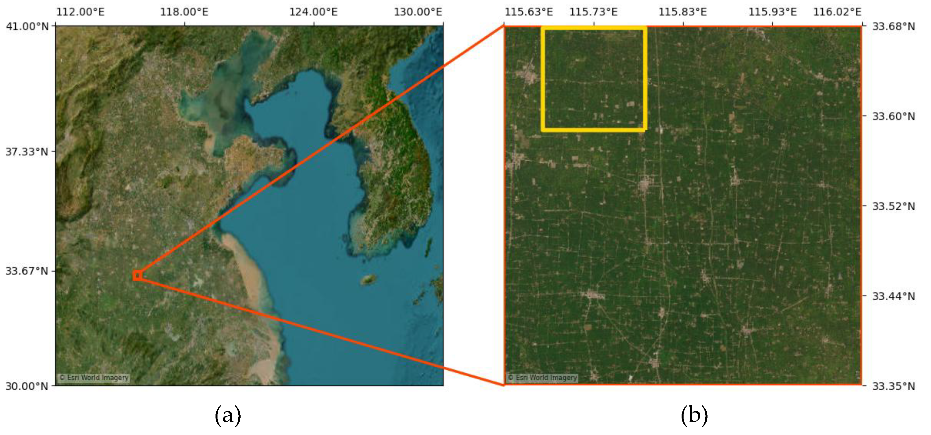
Figure 2.
Flowchart of the NDVI transformation framework used in this study for converting GOCI-II NDVI into MSI–equivalent NDVI.
Figure 2.
Flowchart of the NDVI transformation framework used in this study for converting GOCI-II NDVI into MSI–equivalent NDVI.
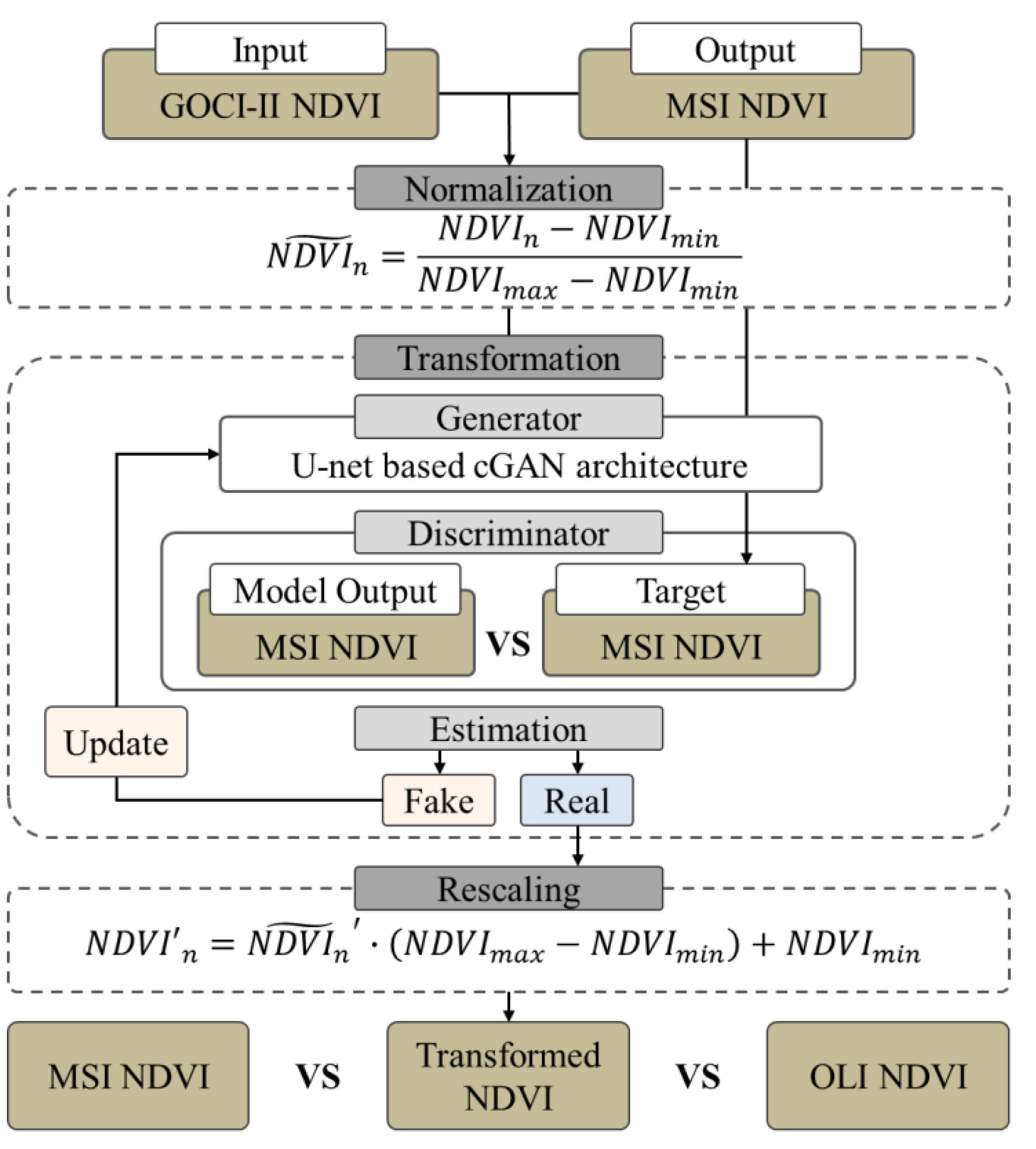
Figure 3.
Spatial comparison of NDVI for the case acquired on 13 January 2025: (a) GOCI-II NDVI, (b) transformed NDVI, (c) reference MSI NDVI, and (d) difference between transformed NDVI and reference MSI NDVI.
Figure 3.
Spatial comparison of NDVI for the case acquired on 13 January 2025: (a) GOCI-II NDVI, (b) transformed NDVI, (c) reference MSI NDVI, and (d) difference between transformed NDVI and reference MSI NDVI.
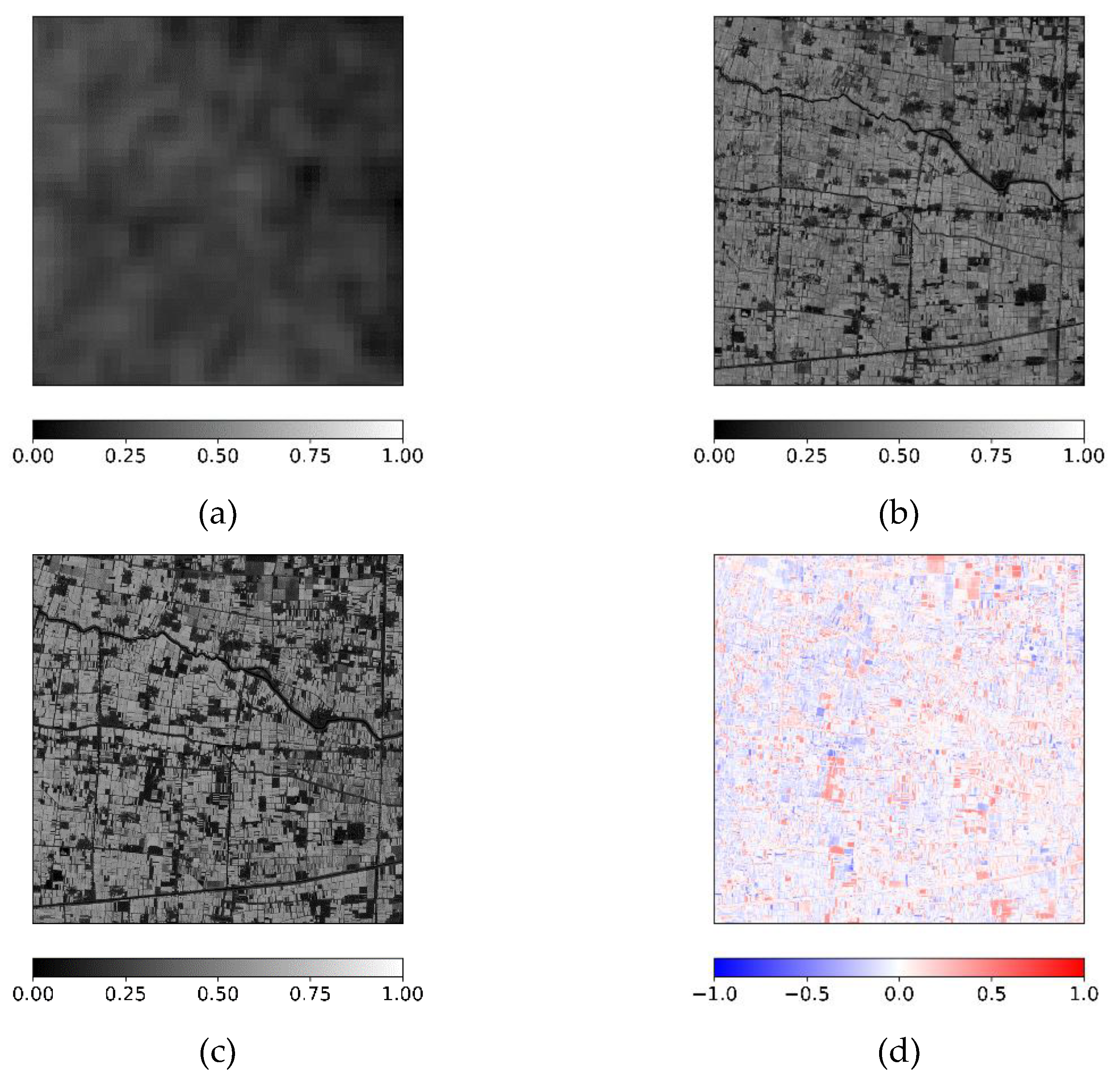
Figure 4.
Spatial comparison of NDVI for the case acquired on 19 March 2025: (a) GOCI-II NDVI, (b) transformed NDVI, (c) reference MSI NDVI, and (d) difference between transformed NDVI and reference MSI NDVI.
Figure 4.
Spatial comparison of NDVI for the case acquired on 19 March 2025: (a) GOCI-II NDVI, (b) transformed NDVI, (c) reference MSI NDVI, and (d) difference between transformed NDVI and reference MSI NDVI.
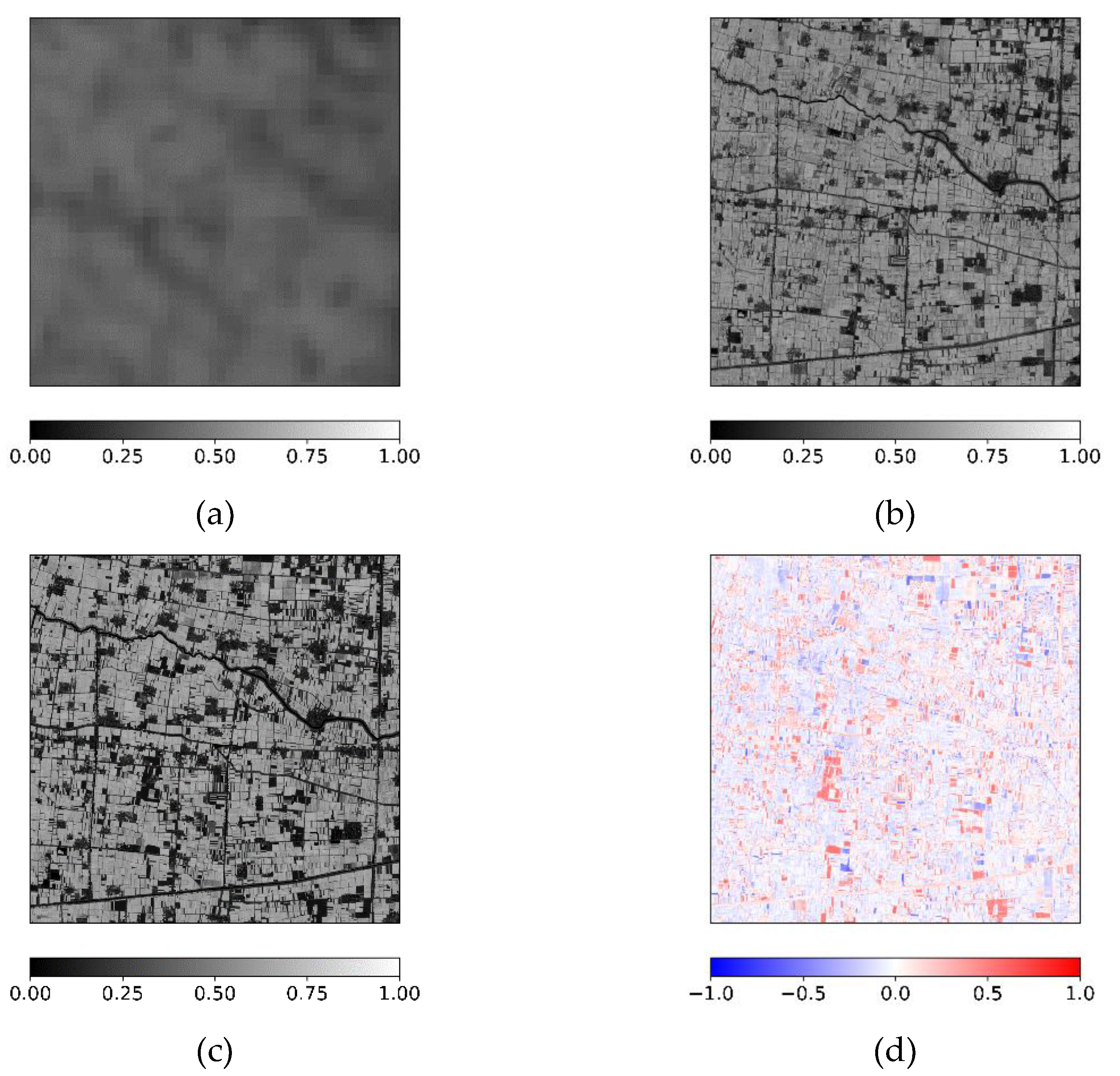
Figure 5.
Cross-sensor comparison of NDVI at 30m resolution for the case acquired on 19 March 2025: (a) NDVI transformed from GOCI-II, (b) MSI NDVI, and (c) OLI NDVI.
Figure 5.
Cross-sensor comparison of NDVI at 30m resolution for the case acquired on 19 March 2025: (a) NDVI transformed from GOCI-II, (b) MSI NDVI, and (c) OLI NDVI.
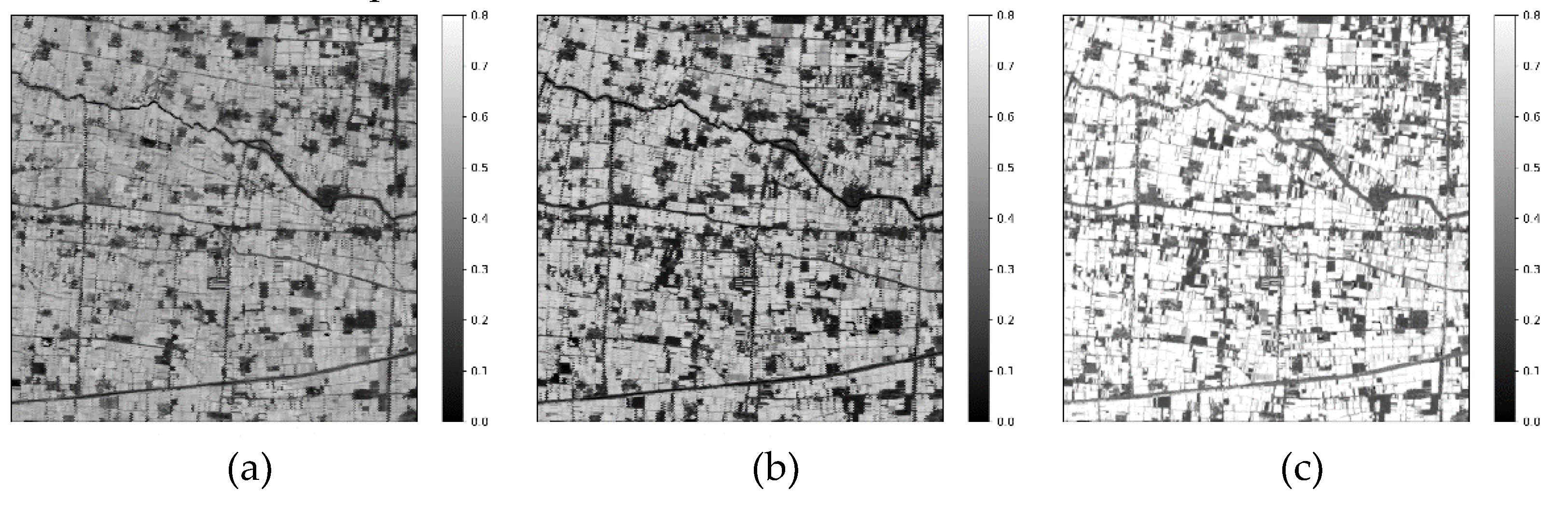
Figure 6.
Cross-sensor comparison of NDVI at 30m resolution for the case acquired on 28 April 2025: (a) NDVI transformed from GOCI-II, (b) MSI NDVI, and (c) OLI NDVI.
Figure 6.
Cross-sensor comparison of NDVI at 30m resolution for the case acquired on 28 April 2025: (a) NDVI transformed from GOCI-II, (b) MSI NDVI, and (c) OLI NDVI.
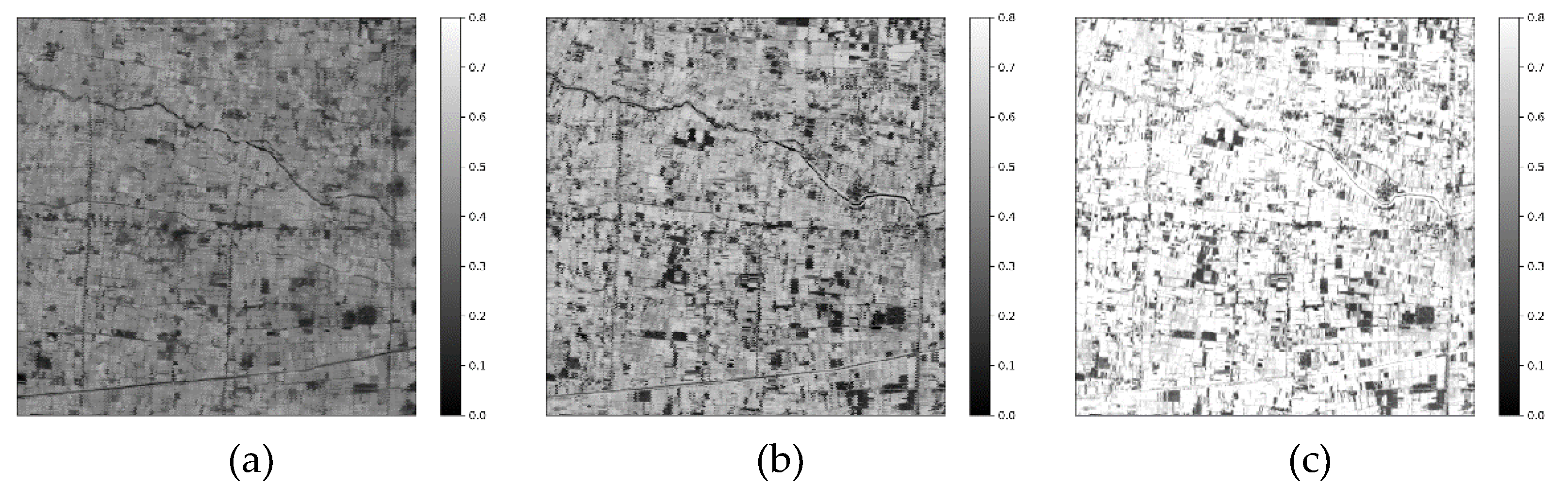
Figure 7.
Example of NDVI gap filling on 28 May 2025. (a) MSI NDVI at 02:55 UTC; (b) gap-filled MSI NDVI using transformed NDVI at 03:15 UTC; (c) gap-filled MSI NDVI using transformed NDVI at 03:15 and 02:15 UTC; (d) cloud-masked MSI NDVI; (e) cloud-masked transformed NDVI at 03:15 UTC; (f) cloud-masked transformed NDVI at 02:15 UTC.
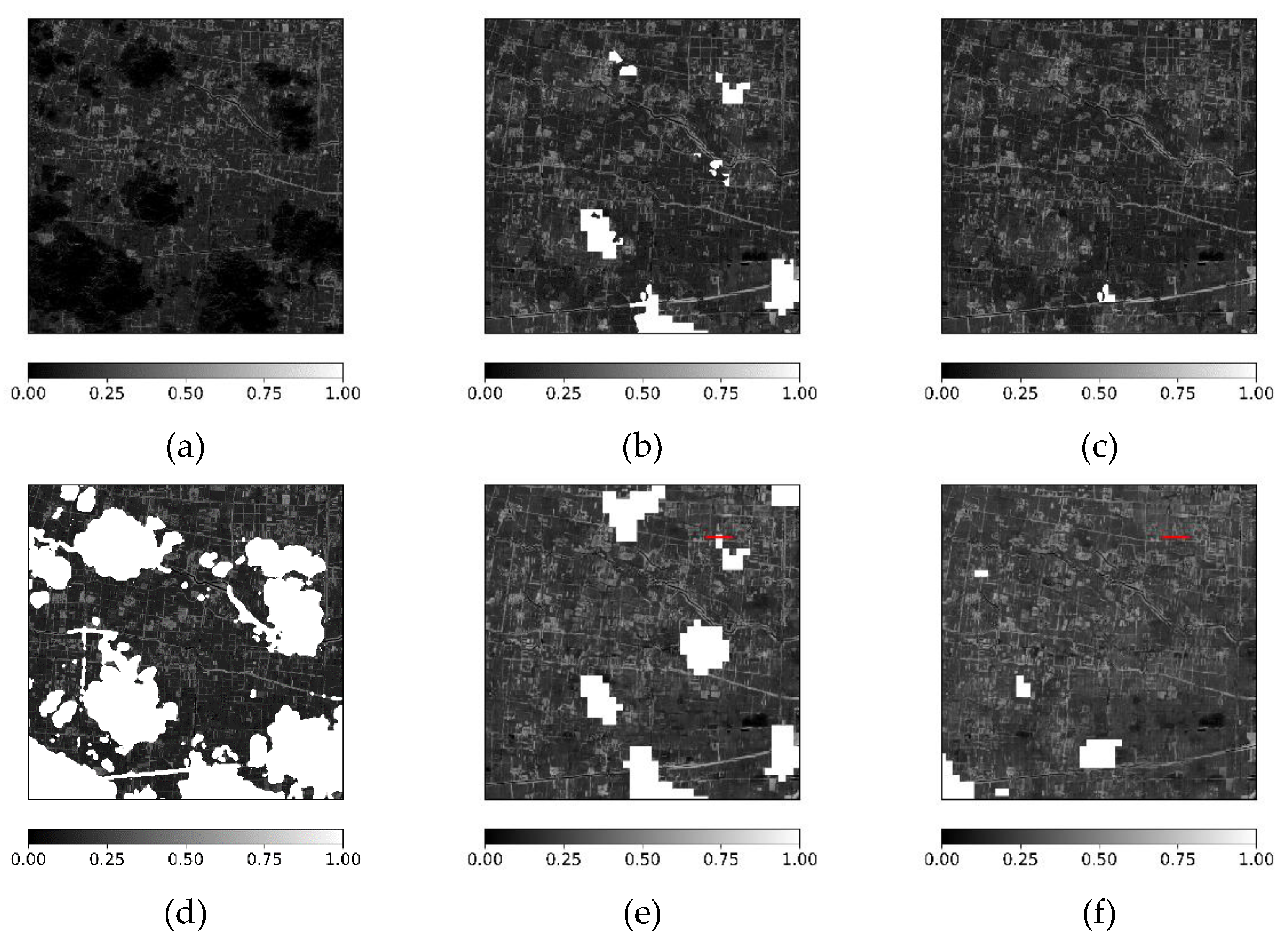
Figure 8.
Trend analysis of transformed NDVI at 02:15 and 03:15 UTC over regions affected by cloud-induced gaps.
Figure 8.
Trend analysis of transformed NDVI at 02:15 and 03:15 UTC over regions affected by cloud-induced gaps.
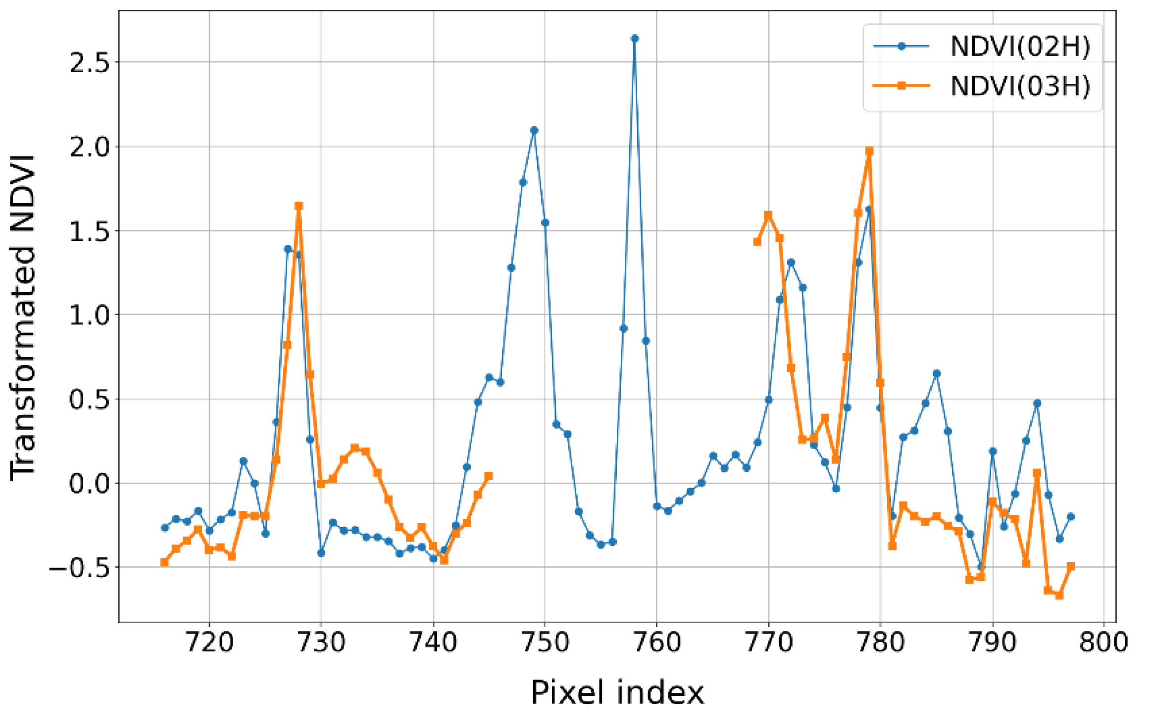
Figure 9.
NDVI comparison over vegetated areas for the case on 19 March 2025, showing (a) transformed NDVI, (b) MSI NDVI, and (c) their difference after removing non-vegetated regions.
Figure 9.
NDVI comparison over vegetated areas for the case on 19 March 2025, showing (a) transformed NDVI, (b) MSI NDVI, and (c) their difference after removing non-vegetated regions.
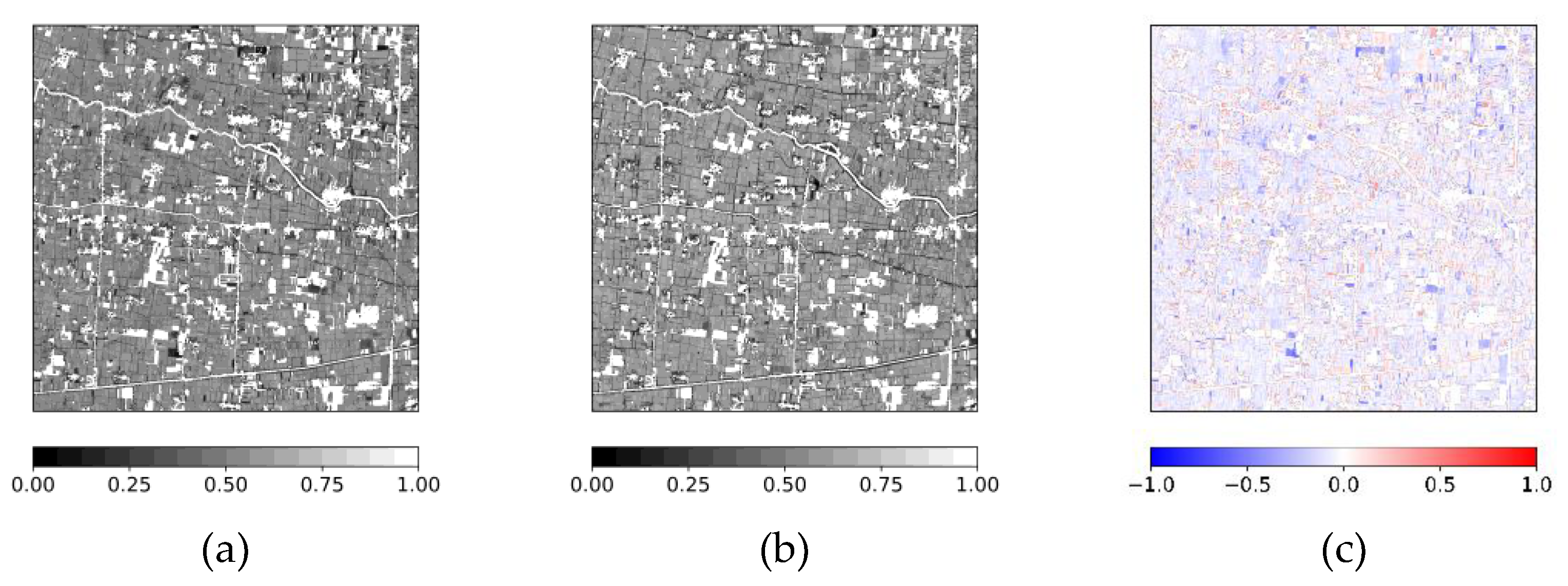
Figure 10.
Density scatter plots comparing transformed NDVI and MSI NDVI for (a) the full study area and (b) non-vegetated regions on 19 March 2025.
Figure 10.
Density scatter plots comparing transformed NDVI and MSI NDVI for (a) the full study area and (b) non-vegetated regions on 19 March 2025.
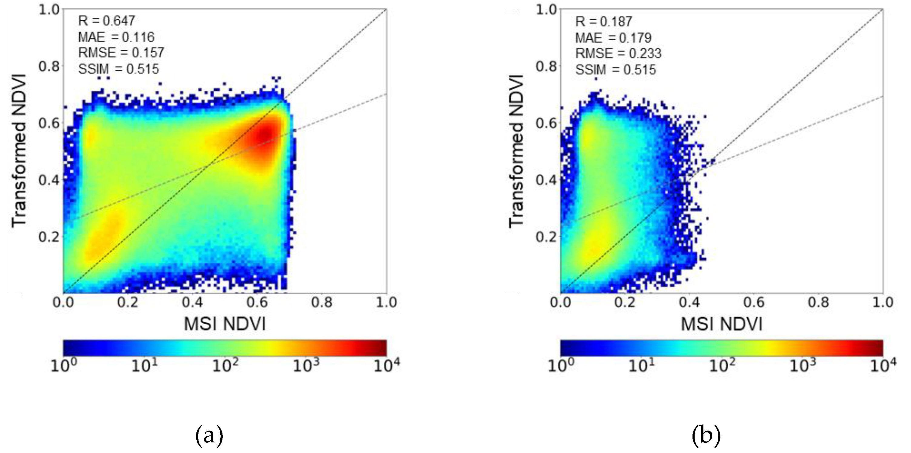
Figure 11.
Comparison of NDVI transformation at an intermediate spatial resolution (80 m) for the 19 March 2025 case, showing (a) transformed NDVI from GOCI-II, (b) MSI NDVI, (c) difference between transformed NDVI and MSI NDVI, and (d) the corresponding density scatter plot.
Figure 11.
Comparison of NDVI transformation at an intermediate spatial resolution (80 m) for the 19 March 2025 case, showing (a) transformed NDVI from GOCI-II, (b) MSI NDVI, (c) difference between transformed NDVI and MSI NDVI, and (d) the corresponding density scatter plot.
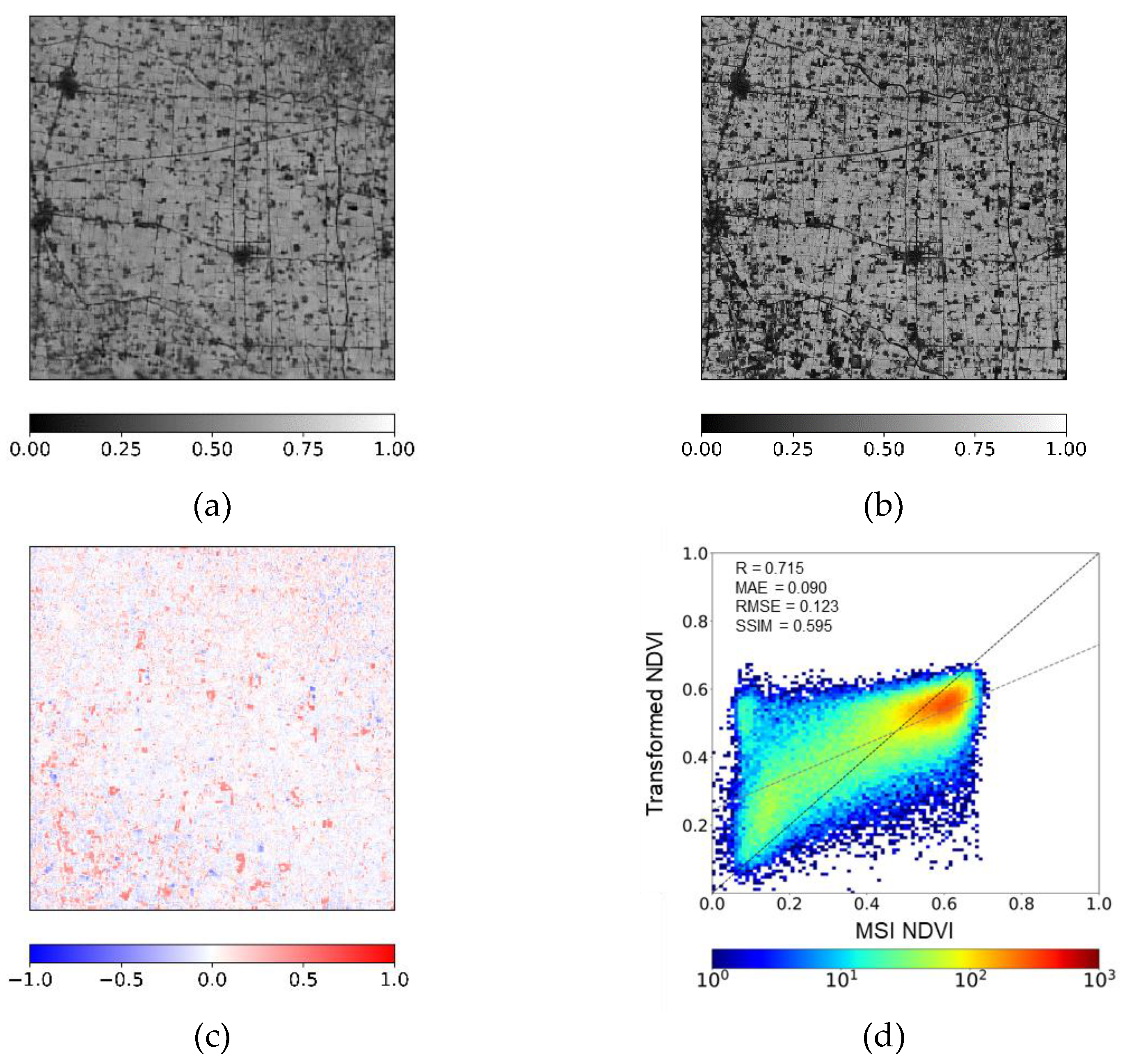

Table 1.
Spectral band characteristics of the GK-2B GOCI-II, Sentinel-2 MSI, and Landsat OLI sensors used in this study.
Table 1.
Spectral band characteristics of the GK-2B GOCI-II, Sentinel-2 MSI, and Landsat OLI sensors used in this study.
| Sensor | Band |
Central Wavelength(nm) |
Resolution(m) |
| GK-2B GOCI-II | Band 8 | 660 | 250 |
| Band 12 | 865 | ||
| Sentinel-2 MSI | Band 4 | 665 | 10 |
| Band 8 | 842 | ||
| Landsat OLI | Band 4 | 655 | 30 |
| Band 5 | 865 |
Table 2.
Representative NDVI values used to characterize different land cover types.
| Land Cover Types | NDVI Threshold |
| Water | -0.046 |
| Bare soil | 0.25 |
| Sparse vegetation | 0.35 |
| Moderate vegetation | 0.5 |
| Dense vegetation | 1.0 |
Table 3.
Statistical metrics for quantitative comparison between transformed NDVI and MSI NDVI.
| Metric | R | MAE | RMSE | SSIM |
| Value | 0.511 | 0.108 | 0.139 | 0.514 |
Disclaimer/Publisher’s Note: The statements, opinions and data contained in all publications are solely those of the individual author(s) and contributor(s) and not of MDPI and/or the editor(s). MDPI and/or the editor(s) disclaim responsibility for any injury to people or property resulting from any ideas, methods, instructions or products referred to in the content. |
© 2026 by the authors. Licensee MDPI, Basel, Switzerland. This article is an open access article distributed under the terms and conditions of the Creative Commons Attribution (CC BY) license (http://creativecommons.org/licenses/by/4.0/).
Copyright: This open access article is published under a Creative Commons CC BY 4.0 license, which permit the free download, distribution, and reuse, provided that the author and preprint are cited in any reuse.


