
Submitted:
25 July 2025
Posted:
28 July 2025
You are already at the latest version
Abstract
Various fusion methods of optical satellite images were proposed for monitoring heterogeneous farmlands requiring high spatial and temporal resolution. In this study, 3m normalized difference vegetation index (NDVI) was generated by applying spatiotemporal fusion method to simultaneously generate full-length normalized difference vegetation index time series (SSFIT) and enhanced spatial and temporal adaptive reflectance fusion method (ESTARFM), to NDVI of Sentinel-2 (S2) and PlanetScope (PS) from 2019 to 2021 for rice paddy and heterogeneous cabbage fields. Before fusion, S2 was applied with the maximum NDVI composite (MNC) and the spatio-temporal gap-filling technique to minimize the cloud effects. The fused NDVI image had a spatial resolution similar to PS, enabling more accurate monitoring of small and heterogeneous fields. In particular, the SSFIT technique showed higher accuracy than ESTARFM with a root mean square error of less than 0.16 and correlation of more than 0.8 compared to PS NDVI, and was processed faster than the ESTARFM code. In some images where ESTARFM was applied, outliers originating from the S2 were still present and heterogeneous NDVI distributions were also shown. This spatio-temporal fusion (STF) technique can be used to produce high-resolution NDVI images for any date during the rainy season required for time-series analysis.
Keywords:
spatio-temporal fusion
; SSFIT
; ESTARFM
; PlanetScope
; Sentinel-2
; NDVI
; rice paddy
; cabbage fields
1. Introduction
As of 2023, the total agricultural area in Korea was reported to be 1,505 thousand ha, of which rice paddies account for 761 thousand ha and fields account for 744 thousand ha [1]. Looking at the growing stages of rice in Korea, the preparation of seedbeds and transplanting of rice seedlings takes place from mid-April to early June, full-scale growth takes place from June to August, and harvesting takes place from mid-September to early October. Rice is an annual crop, and it takes 3 to 6 months from germination to growth, heading, and maturation [2]. In particular, the crops grown in Korean fields are very diverse, and the cultivated area for each crop is very small, less than 1 ha per farm household, and various items are grown scattered throughout the country [3]. In order to remotely monitor Korea’s small-scale and diverse farmland, an optical satellite with high spatial and temporal resolution is required. Accordingly, the Compact Advanced Satellite 500-4 (CAS500-4), an agricultural and forestry satellite, scheduled to be launched in 2026, is designed to monitor the Korean Peninsula with a spatial resolution of 5 m and a three-day cycle.
More accurate monitoring of crops is needed during the summer season when most crops grow rapidly, but this period overlaps with the rainy season, limiting the use of optical satellite images for crop monitoring [4,5,6]. As a solution to this problem, a cloud-free composite algorithm was proposed that collects low- and medium-resolution satellite images over a certain period of time to create a single representative image with minimal cloud influence [7]. Cloud-free composite algorithm can be divided into a method for selecting pixels with minimal cloud influence over a certain period and a method for generating new representative pixel values. However, in the case of crop monitoring, a method for selecting optimal pixels is more useful in that the spectral information of the original image is maintained [6]. In particular, among various optimal pixel selection methods, the MNC algorithm is most widely applied in many optical satellite images, including NOAA-AVHRR and Terra/Aqua MODIS, because the processing process is simple and the cloud removal effect is high [7,8,9].
When cloud removal is not complete due to the large amount of cloud cover during the long rainy season, or when monitoring time-series changes in crops, algorithm for restoring missing data is applied. This type of algorithm is referred to as the gap-filling method, and can be divided into temporal interpolation (or smoothing techniques) and spatial filling [10]. In the case of MODIS, it provides the Gap-Filled, Smoothed (GFS) product that applies these two gap-filling techniques, and in the case of S2, it provides various temporal missing correction techniques through a missing correction program called Decomposition and Analysis of Time Series (DATimeS) software [10,11]. In a previous study, spatial and temporal gap-filling software for NDVI images from S2 satellites was developed for the Korean rice paddy area, and this software presented an RMSE of less than 0.15 [12]. Recently, high-resolution satellite constellation such as PS have been utilized for crop monitoring [13,14,15,16], and although they can be taken at short intervals using multiple satellites, there are limitations such as the difficulty in generating time series data due to the cost [17]. In addition, differences occur between satellite constellation, and additional normalization may be required for wide-area monitoring or time series analysis [18,19].
Satellite sensors with various resolutions are provided, and various fusion techniques between multiple satellite images have been proposed to resolve the trade-off between resolutions [20,21]. For example, the STF algorithm was applied to Landsat series and MODIS data to produce high spatial resolution reflectance data for a desired date to monitor crop growth [21,22]. STF algorithms can be broadly divided into pair-based fusion methods such as Spatial and Temporal Adaptive Reflectance Fusion Method (STARFM) [20], Enhanced STARFM (ESTARFM) [23], and regression model Fitting, spatial Filtering and residual Compression (Fit-FC) [24], and time-series-based fusion methods such as SSFIT [21,22]. The pair-based method is a technique that generates fusion data with dates similar to those of input data based on the statistical relationship between input pair data. It is simple to apply, but its accuracy varies depending on the number or distribution of input data, and it has the disadvantage of not considering temporal pattern characteristics [21]. On the other hand, SSFIT can generate high-resolution images of a desired date without high-resolution satellite images that are not affected by clouds, and requires a time series pattern to be input [22]. These fusion methods were developed based on reflectance and have recently been applied to MODIS and Landsat NDVI, suggesting their potential for use [22]. Recently, there has been an increase in the number of cases of fusing PS and S2 for crop monitoring, but most of them have been applied using spatio-spectral fusion methods, and there have been no cases where a fusion method for time series analysis has been applied [25,26,27].
This study applied the spatio-temporal gap-filling method to the S2 images acquired from 2019 to 2021, which showed various precipitation amounts over relatively wide and homogeneous rice fields and narrow and heterogeneous cabbage fields, to generate S2 NDVI with fewer missing values and improved temporal consistency, and then apply two representative fusion methods (SSFIT and ESTARFM) to these data and the PS data, respectively. Through this, we produce 3m NDVI on a desired date, and compare the fusion results of the two methods to suggest a fusion method suitable for small and heterogeneous farmland.
2. Materials and Methods
2.1. Study Area and Data Used
The study area was selected as the main agricultural land in Korea, which is rice paddies and dry fields. In the case of fields, the type of crop often changes every year, so a highland cabbage field that grows the same crop every year was selected for time series analysis. The rice paddy area was selected as Waemok Village, Dangjin, Chungcheong Province (Figure 1 (a)), and rice planting began in May and harvesting began in October. As shown in Figure 1, the rice paddy area shows a relatively homogeneous distribution compared to the fields. Another study area is the highland cabbage field in Maebongsan, Taebaek, Gangwon-do (Figure 1 (b)). Because it is a high-altitude area, only cabbage is cultivated, and the planting and cultivation periods differ depending on the owner of each plot. Cabbage is planted in May to June and harvested in August to September. Recently, the region has been suffering from soft rot due to the effects of global warming, which has led to a decrease in harvest.
S2, a medium-resolution satellite with high periodic resolution, and PS, a high-resolution satellite, were used to collect images in the two study areas. S2 Level 2A images provide a spatial resolution of 10 m, and are taken by two satellites intersecting each other, providing images of the same area every five days. This is an atmospheric-corrected L2A reflectance image using Sen2Cor software, provided by the Copernicus Open Access Hub (https://scihub.Copernicus.eu/dhus/). The red band (650-680 nm) and near-infrared band (785-899 nm) of S2 are used to derive time-series NDVI patterns. Another data to be used for fusion is PS L3B, a satellite constellation image data that provides a spatial resolution of 3m and can be taken on any desired date, but requires a fee. PS reflectance data is data that has undergone 6SV-based atmospheric correction, and NDVI was created using the reflectance of the red band (650-680 nm) and the near-infrared band (845-885 nm). PS NDVI images are divided into training data input to the STF model and test data to verify the accuracy of the fusion result.
The target period was selected as May to October according to the growing cycle of the rice paddy, and May to September for the fields. In addition, data from 2019 and 2021 showing average precipitation and data from 2020 showing about 200 mm higher precipitation than the average from July to October were used as shown in Table 1 for time series analysis [5].
2.2. Methods
In order to fuse S2 time series NDVI data with PS data providing 3m NDVI, this study applied representative STF methods, SSFIT and ESTARFM, respectively. As shown in Figure 2, preprocessing is performed to input each STF method. Verification was performed using the data fused by the two methods and the PS test data. The following contents described in detail the preprocessing process (2.2.1) and two STF methods (2.2.2 and 2.2.3) of the two satellite images, and the verification method (2.2.4) of the two results.
2.2.1. Preprocessing
After generating NDVI using the red and near-infrared bands of the S2 L2A data, data is acquired every 15 days, and a MNC process is performed to create a representative image with pixels showing the maximum NDVI per pixel to minimize the influence of clouds. To minimize missingness due to remaining cloud areas, a spatial gap-filling process is performed to replace missing pixels with the average NDVI of nearby pixels in small missing areas of 5 pixels or less. Next, Gaussian Process Regression (GPR), the most commonly used technique for temporal gap-filling, was performed, which requires two images taken before the missing date and one image taken after it [11]. This spatio-temporal gap-filling technique has been modularized and used in Python, showing an RMSE of 0.173 and taking 5 minutes of processing time per scene [12]. Through this, S2 time series NDVI data from 2019 to 2021 with minimal cloud impact were generated, and S2 data to be used for two STF methods were prepared. The S2 time series NDVI data from 2019 to 2021, when the cloud impact was minimized, were resampled to 3 m to match the PS data and inputted into two STF models. The PS2 L3B data was also used to generate NDVI image using two bands, and was divided into training data used as input data for two fusion models and test data used to verify the fusion methods. The following 2.2.2 and 2.2.3 describe two types of STF methods.
2.2.2. SSFIT Method
The SSFIT is a fusion algorithm developed based on time series MODIS and Landsat EVI data, and presents relatively higher accuracy than other STF methods in crop monitoring [21,22]. First, SVD (Singular Value Decomposition) transformation is applied to derive base (bi) representing the pattern of time series NDVI from time series S2 data. Through SVD transformation, an orthogonal matrix providing spatial information of S2, a diagonal matrix composed of singular values, and bases, which are right-singular row vectors providing time series information, are derived. In this study, bi was derived by year. Next, by inputting PS NDVI (f) and the base (bi) of S2 into Equation 1, base coefficients (ai) are calculated using the least squares method.
where f(x, y, t) is the PS NDVI value of the pixel located at (x, y) observed on date t, bi(x, y, t) is the ith base obtained from S2, ai(x, y) is base coefficients of the ith base, nb is the number of the bases, and ε is the model residual [22].
The coefficients are calculated for each pixel, and the 3m NDVI image for a desired date are generated using these coefficients, which are implemented in Python.
2.2.3. ESTARFM Method
ESTARFM is an algorithm that combines spectral mixing analysis with STARFM, a representative weight-based fusion algorithm, to achieve higher accuracy in heterogeneous regions [23,28]. A search window is set to search for spatially adjacent neighboring pixels at the predicted location, and the spatial, spectral, and temporal similarities between the input S2 and PS pair data and the PS data of the predicted date are calculated as weights. When the search window size is w, the 3m high-resolution NDVI value at the center pixel (xw/2, yw/2) of the search window on the prediction date tp is predicted as the sum of the weighted input data as in Equation 2.
where k is the number of pairs of S2 and PS data acquired on the same date tk, f is S2 NDVI, c is PS NDVI image, and Tk is the temporal weight for the intensity of change in the time series NDVI. W is the weight for spatial and spectral information, and a high weight is assigned to data that exhibits similar spectral characteristics and are spatially close within the search window. v is a coefficient that converts S2 to PS, and considers the difference in spatial resolution.
In this study, the Python implementation code of ESTARFM provided on the webpage (https://xiaolinzhu.weebly.com/open-source-code.html) was used.
2.2.4. Validation Method
In this study, two STF fusion results corresponding to the dates of independent PS test data are predicted and compared with the predicted data and PS NDVI test data. To verify whether the actual high-resolution NDVI was generated, a qualitative comparison is performed visually on 10m S2, 3m PS, and fused 3m NDVI. In addition, for quantitative analysis, correlation and RMSE values are calculated based on the PS test data, and time series analysis of S2 time series NDVI, PS, and fused NDVI image is performed. In these qualitative and quantitative validations, this study has various comparative perspectives. First, we analyze which STF method is efficient in heterogeneous areas by comparing the two representative STF results in homogenous rice paddy and heterogeneous fields. In addition, we compare the STF results between 2019 and 2021, which showed normal precipitation, and 2020, which showed high precipitation (high cloud cover).
3. Results
3.1. Qualitative Evaluation of Time-Series Fused NDVI Data
To evaluate the qualitative quality of the NDVI images synthesized by the two techniques, S2, PS, and fused NDVI images were visually compared for rice fields and cabbage fields (Figure 3, Figure 4 and Figure 5). The S2 NDVI image is a composite of data from a 15-day period, and is different from the PS image taken on that date. Looking at the NDVI of the rice paddy area in 2019 (Figure 3), May and June showed very low NDVI due to the rice planting season, then increased until September and decreased after harvest in October. In addition, differences in harvest times by plot were observed. In the highland cabbage fields, NDVI increases significantly between June and July, and NDVI decreases from mid-August when harvest is made. The NDVI difference in cabbage fields by year was large compared to that in rice paddy. The PS and fusion results on both sites mostly showed similar NDVI distributions, but there were differences in NDVI between the images of the paddy field area on July 9, 2019 and September 18, 2019 and the images of the cabbage field area on June 16, 2020 and June 18, 2021. Most of these data were acquired during a period when the rate of vegetation change was rapid. Looking at the time-series NDVI pattern (Figure 6), this difference is caused by a large difference in NDVI of the test data taken at a similar time (<10 days) as the PS training data used for prediction. In addition, for the cabbage fields in 2020 and 2021, where the number of PS training images was small, the differences between the fused and the PS test NDVI images increased (Figure 5 and 6).
In addition, when examining the partial images (Figure 3, Figure 4 and Figure 5), improved spatial resolution was confirmed in the 3m fused NDVI image compared to the 10m S2 NDVI image, and more detailed boundaries were shown, especially in the cabbage field. Comparing the results of the two fusion methods, we can see that the influence of the remaining clouds in S2 on September 18, 2019 was also observed in ESTARFM. In addition, ESTARFM showed areas that were not predicted or had an inhomogeneous NDVI distribution compared to SSFIT results on specific dates. This is a phenomenon that occurs because ESTARFM estimates only using NDVI near the forecast date, unlike SSFIT, which utilizes time series pattern information, and thus the quality information of the data used is directly reflected.
Looking at the time-series average NDVI pattern (Figure 6), the year 2020, when rainfall was high in both rice paddies and dry fields, shows a different time-series S2 NDVI pattern compared to other normal years (2019 and 2021). In comparison, PS NDVI, which is captured only on days with good weather, shows a similar NDVI pattern every year, and time-series NDVI monitoring of crops in rice paddies and cabbage fields is possible even during the rainy season through a fusion technique that can generate NDVI image of a desired period.
3.2. Quantitative Evaluation of Two STF Results Using PS Test Images
To quantitatively evaluate the fused NDVI image, the one-to-one correspondence distribution, correlation, and RMSE with the PS test NDVI image were calculated. As shown in Table 2 and Table 3, the STF results in the rice paddy area showed an RMSE of 0.02 to 0.16 and a correlation of 0.80 or higher based on the PS test NDVI image, while in the cabbage fields, the RMSE was lower than 0.1 and a high correlation of 0.87 or higher was shown.
Although accuracy differences are small, the scatter plot shows that SSFIT is distributed closer to a one-to-one line than ESTARFM, is more coherent, and has a lower RMSE (Figure 7).
For SSFIT, it took 4 seconds to process based on NDVI image in the rice paddy, and ESTARFM took 5 minutes to process. The tested PC specifications are AMD Ryzen 9 5900X 12-Core Processor 3.70 GHz, RAM DDR5 PC5-44800 128GB and GPU NVIDIA GeForce RTX 3060 Ti. The ESTARFM code took a certain amount of processing time because it was a process of calculating similarity between input images through a search window.
4. Discussion
This study attempted STF with S2 by utilizing more PS data compared to other studies, and was able to present effective fusion results. However, due to practical limitations such as cost issues, questions are raised about the applicability of the STF technique when less PS data is obtained. In theory, if two or more PS data are used, prediction is possible, but the accuracy may be relatively low. In addition, if a large number of PS images can be observed, a method can be proposed to use them directly for time series monitoring without additional fusion. However, as shown in this time series NDVI pattern, PS NDVI shows a large variability in NDVI values with a difference of several days, which causes problems in analyzing a stable time series NDVI pattern compared to S2 NDVI. Therefore, it can be said that predicting NDVI on a desired date by a STF technique such as SSFIT is more useful. In addition, 2019, which had a small amount of data, showed slightly lower accuracy than 2020, which had a large amount of data, and 2021, which had a similar amount of data to 2019, showed relatively higher accuracy than 2019 because the data was concentrated until August. In this way, the number and distribution of many data affect the prediction accuracy of the STF result. Accordingly, additional analysis is needed on how the distribution and number of training data used for STF method quantitatively affect the prediction accuracy of the fusion data. In addition, in terms of processing speed, SSFIT processes in a very short time, but considering the time required to construct time series data, it requires a lot of manpower and time, so this needs to be taken into consideration.
5. Conclusions
Two representative STF methods, SSFIT and ESTARFM, were applied to S2 and PS NDVI to produce 3m NDVI image for the desired date. The results of applying both techniques showed similar spatial resolution and NDVI distribution to PS data. The fused data provided more detailed NDVI information in the heterogeneous field with improved spatial resolution. Compared with the ESTARFM method, the SSFIT method provided more accurate and homogeneous NDVI information by reflecting the time series NDVI information throughout the year, which was less affected by errors or inaccuracies in the input data. In addition, SSFIT’s processing speed is fast, so it can be used more efficiently. While it is difficult to obtain clear images during the rainy season with S2 acquired periodically, NDVI on a desired day can be estimated through fusion with PS images acquired on clear days, making time-series NDVI analysis easier. In the future, quantitative analysis will be conducted on how the number and distribution of input data affect the STF results.
Author Contributions
Methodology, S.-H.K.; Software, I.B.; Analysis, J.E. and S.-H.K.; data curation, J.E.; Manuscript preparation J.E. and S.-H.K.; Manuscript review and editing, T.-H. K. and S.-H.K.; visualization, I.B.; project administration, T.-H. K.; funding acquisition, T.-H. K. All authors have read and agreed to the published version of the manuscript.
Funding
This paper was supported by the Rural Development Administration Joint Research Project (Project No. PJ0162342025) and is gratefully acknowledged.
Institutional Review Board Statement
Not applicable.
Informed Consent Statement
Not applicable.
Data Availability Statement
The data presented in this study are available on request from the corresponding author. (please specify the reason for restriction, e.g., the data are not publicly available due to privacy or ethical restrictions.)
Acknowledgments
The authors would like to thank the Polyu Remote sensing Intelligence for Dynamic Earth (PRIDE) Laboratory (Dr. Xiaolin Zhu) for providing the ESTARFM code.
Conflicts of Interest
The authors declare no conflicts of interest.
Abbreviations
The following abbreviations are used in this manuscript:
| NDVI | Normalized Difference Vegetation Index |
| STF | Spatio-Temporal Fusion |
| SSFIT | Spatiotemporal fusion method to Simultaneously generate Full-length normalized difference vegetation Index Time series |
| ESTARFM | Enhanced Spatial and Temporal Adaptive Reflectance Fusion Method |
| S2 | Sentinel-2A/B |
| PS | PlanetScope |
| MNC | Maximum NDVI Composite |
| RMSE | Root Mean Square Error |
References
- Korean Statistical Information Service. Available online: https://kosis.kr (accessed on 25 June 2025).
- Rural Development Administration. Available online: https://www.rda.go.kr/board/board.do?mode=view&prgId=day_farmprmninfoEntry&dataNo=100000749546 (accessed on 25 June 2025).
- newsFM. Available online: https://www.newsfm.kr/mobile/article.html?no=7021 (accessed on 25 June 2025).
- Griffiths, P.; Nendel, C.; Hostert, P. Intra-annual reflectance composites from Sentinel-2 and Landsat for national-scale crop and land cover mapping. Remote Sensing of Environment 2019, 220, 131–151. [Google Scholar] [CrossRef]
- Eun, J.; Kim, S.H.; Kim, T.H. Analysis of the cloud removal effect of Sentinel-2A/B NDVI monthly composite images for rice paddy and high-altitude cabbage fields. Korean Journal of Remote Sensing 2021, 37, 1545–1557. [Google Scholar] [CrossRef]
- Kim, S.H.; Eun, J. Development of score-based vegetation index composite algorithm for crop monitoring. Korean Journal of Remote Sensing 2022, 38, 1343–1356. [Google Scholar] [CrossRef]
- Wang, L.; Xiao, P.; Feng, X.; Li, H.; Zhang, W.; Lin, J. Effective compositing method to produce cloud-free AVHRR image. IEEE Geoscience and Remote Sensing Letters 2014, 11, 328–332. [Google Scholar] [CrossRef]
- Holben, B.N. Characteristics of maximum-value composite images from temporal AVHRR data. International Journal of Remote Sensing 1986, 7, 1417–1434. [Google Scholar] [CrossRef]
- Fraser, A.D.; Masson, R.A.; Michael, K.J. A method for compositing polar MODIS satellite images to remove cloud cover for landfast sea-ice detection. IEEE Transactions on Geoscience and Remote Sensing 2009, 47, 3272–3282. [Google Scholar] [CrossRef]
- Gao, F.; Morisette, J.T.; Wolfe, R.E.; Ederer, G.; Pedelty, J.; Masuoka, E.; et al. An algorithm to produce temporally and spatially continuous MODIS-LAI time series. IEEE Geoscience and Remote Sensing Letters 2008, 5, 60–64. [Google Scholar] [CrossRef]
- Belda, S.; Pipia, L. , Morcillo-Pallarés, P.; Rivera-Caicedo, J.P.; Amin, E.; De Grave, C.; Verrelst, J. DATimeS: A machine learning time series GUI toolbox for gap-filling and vegetation phenology trends detection. Environmental Modelling and Software 2020, 127, 104666. [Google Scholar] [CrossRef]
- Kim, S.H.; Eun, J.; Kim, T.H. Development of spatio-temporal gap-filling technique for NDVI images. Korean Journal of Remote Sensing 2024, 40, 957–963. [Google Scholar] [CrossRef]
- Li, F.; Miao, Y.; Chen, X.; Sun, Z.; Stueve, K.; Yuan, F. In-season prediction of corn grain yield through PlanetScope and Sentinel-2 images. Agronomy 2022, 12, 3176. [Google Scholar] [CrossRef]
- Eun, J.; Kim, S.H.; Min, J.E. Comparison of NDVI in rice paddy according to the resolution of optical satellite images. Korean Journal of Remote Sensing 2023, 39, 1321–1330. [Google Scholar] [CrossRef]
- Planet Pulse. Available online: https://www.planet.com/pulse/next-generation-agriculture-monitoring-at-scale-with-planets-crop-biomass (accessed on 2 July 2025).
- Swain, K.C.; Singha, C.; Pradhan, B. Estimating total rice biomass and crop yield at field scale using PlanetScope imagery through hybrid machine learning models. Earth Systems and Environment 2024, 8, 1713–1731. [Google Scholar] [CrossRef]
- Kumhálová, J.; Matějková, S. ; Yield variability prediction by remote sensing sensors with different spatial resolution. International Agrophysics 2017, 31, 195–202. [Google Scholar] [CrossRef]
- Frazier, A.E.; Hemingway, B.L. ; A technical review of Planet smallsat data: practical considerations for processing and using PlanetScope imagery. Remote sensing 2021, 13, 3930. [Google Scholar] [CrossRef]
- Planet Labs. Available online: https://assets.planet.com/docs/scene_level_normalization_of_planet_dove_imagery.pdf (accessed on 2 July 2025).
- Gao, F.; Masek, J.; Schwaller, M.; Hall, F. On the blending of the Landsat and MODIS surface reflectance: Predicting daily Landsat surface reflectance. IEEE Transactions on Geoscience and Remote Sensing 2006, 44, 2207–2218. [Google Scholar] [CrossRef]
- Tian, J.; Zhu, X. , Shen, M.; Chen, J.; Cao, R.; Qiu, Y.; Xu, Y.N. Effectiveness of spatiotemporal data fusion in fine-scale land surface phenology monitoring: A simulation study. Journal of Remote Sensing, 2024. [CrossRef]
- Qiu, Y.; Zhou, J.; Chen, J.; Chen, X. Spatiotemporal fusion method to simultaneously generate full-length normalized difference vegetation index time series (SSFIT). International Journal of Applied Earth Observations and Geoinformation 2021, 100, 102333. [Google Scholar] [CrossRef]
- Zhu, X.; Chen, J.; Gao, F.; Chen, X.; Masek, J.G. An enhanced spatial and temporal adaptive reflectance fusion model for complex and heterogeneous regions. Remote Sensing of Environment 2010, 114, 2610–2623. [Google Scholar] [CrossRef]
- Wang, Q.; Atkinson, P.M. Spatio-temporal fusion for daily Sentinel-2 images. Remote Sensing of Environment 2018, 204, 31–42. [Google Scholar] [CrossRef]
- Zhao, Y.; Liu, D. A robust and adaptive spatial-spectral fusion model for PlanetScope and Sentinel-2 imagery. Geoscience & Remote Sensing 2022, 59, 520–546. [Google Scholar] [CrossRef]
- Sarker, S.; Sagan, V.; Bhadra, S.; Fritschi, F.B. Spectral enhancement of PlanetScope using Sentinel-2 images to estimate soybean yield and seed composition. Scientific Reports 2024, 14, 15063. [Google Scholar] [CrossRef]
- Gašparović, M.; Medak, D.; Pilaš, I.; Jurjević, L.; Balenović, I. Fusion of Sentinel-a and PlanetScope imagery for vegetation detection and monitoring. The International Archives of the Photogrammetry Remote Sensing and Spatial Information Sciences, 2018, XLII-1, 155-160. [CrossRef]
- Kim, Y.; Park, N.W. Comparison of spatio-temporal fusion models of multiple satellite images for vegetation monitoring. Korean Journal of Remote Sensing 2019, 35, 1209–1219. [Google Scholar] [CrossRef]
Figure 1.
PS natural color composite images of two study areas: (a) Dangjin rice paddy; (b) Taeback cabbage fields.
Figure 1.
PS natural color composite images of two study areas: (a) Dangjin rice paddy; (b) Taeback cabbage fields.
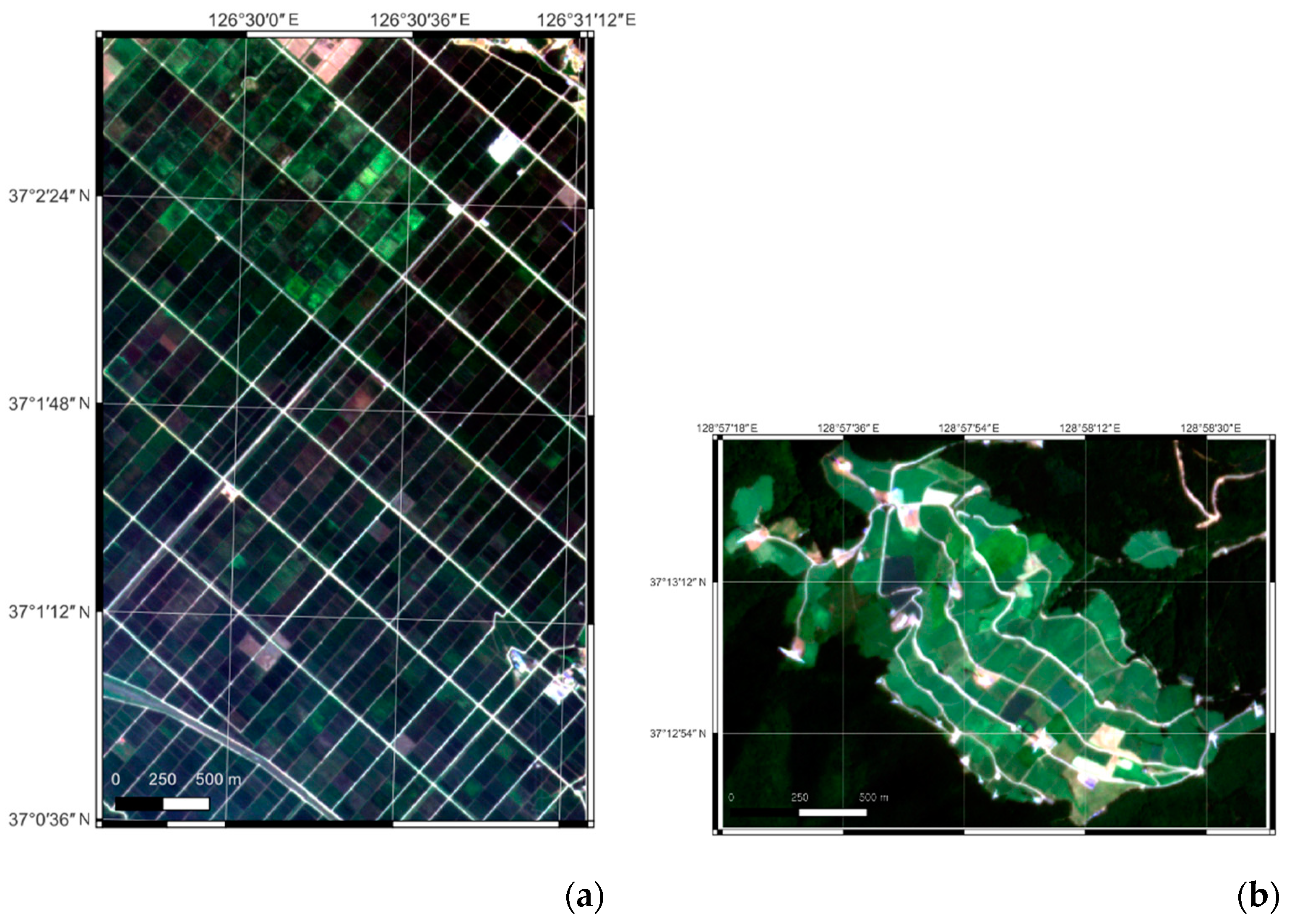
Figure 2.
Flowchart for fusion processing of S2 and PS NDVI images.
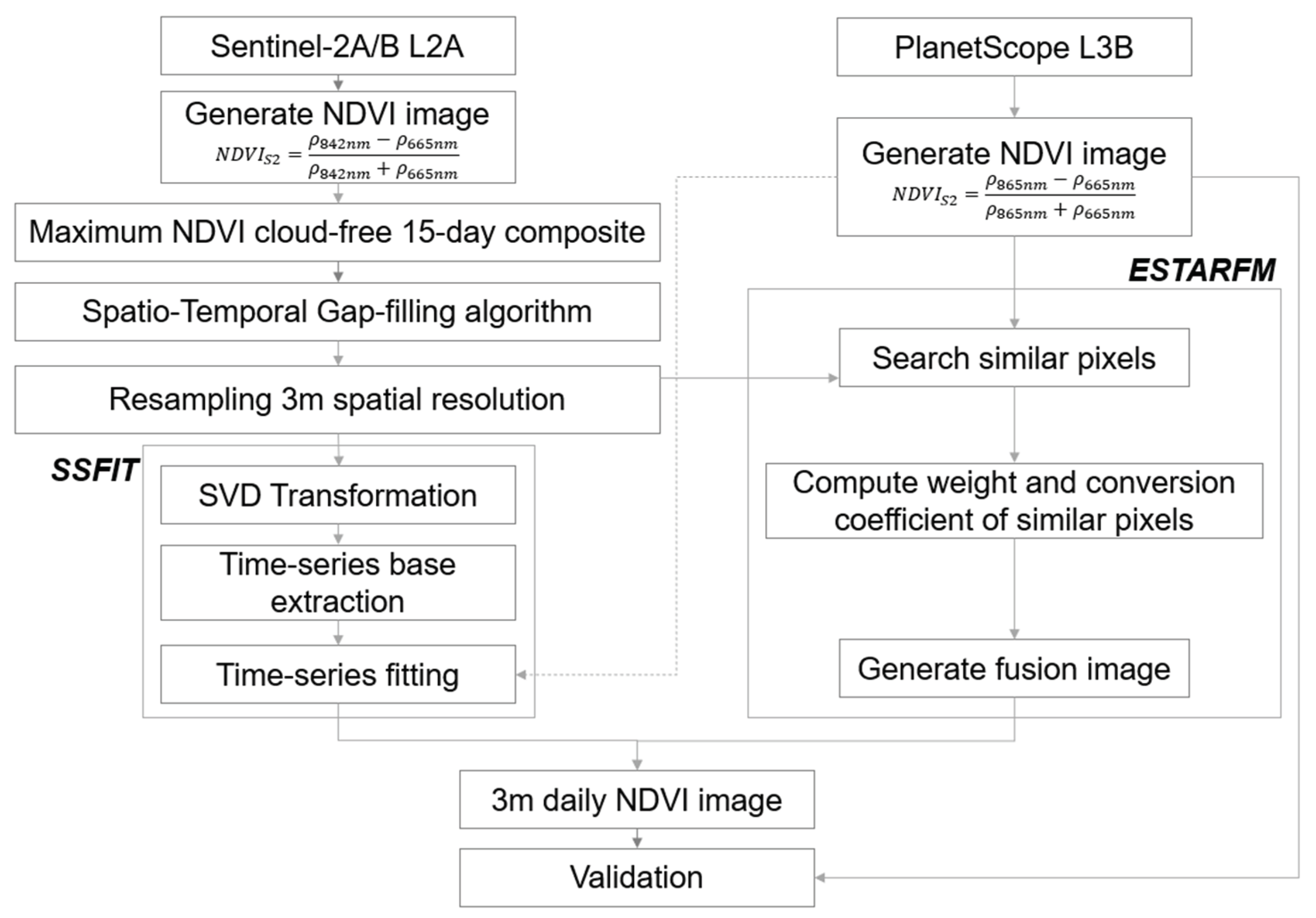
Figure 3.
NDVI images of the rice paddy area on the prediction dates in 2019.
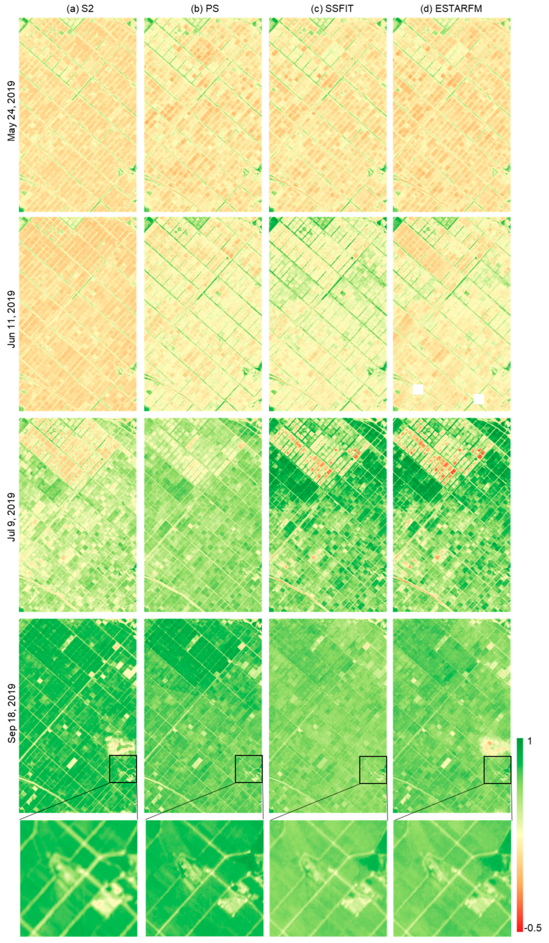
Figure 4.
NDVI images of the rice paddy area on the prediction dates from 2020 to 2021.
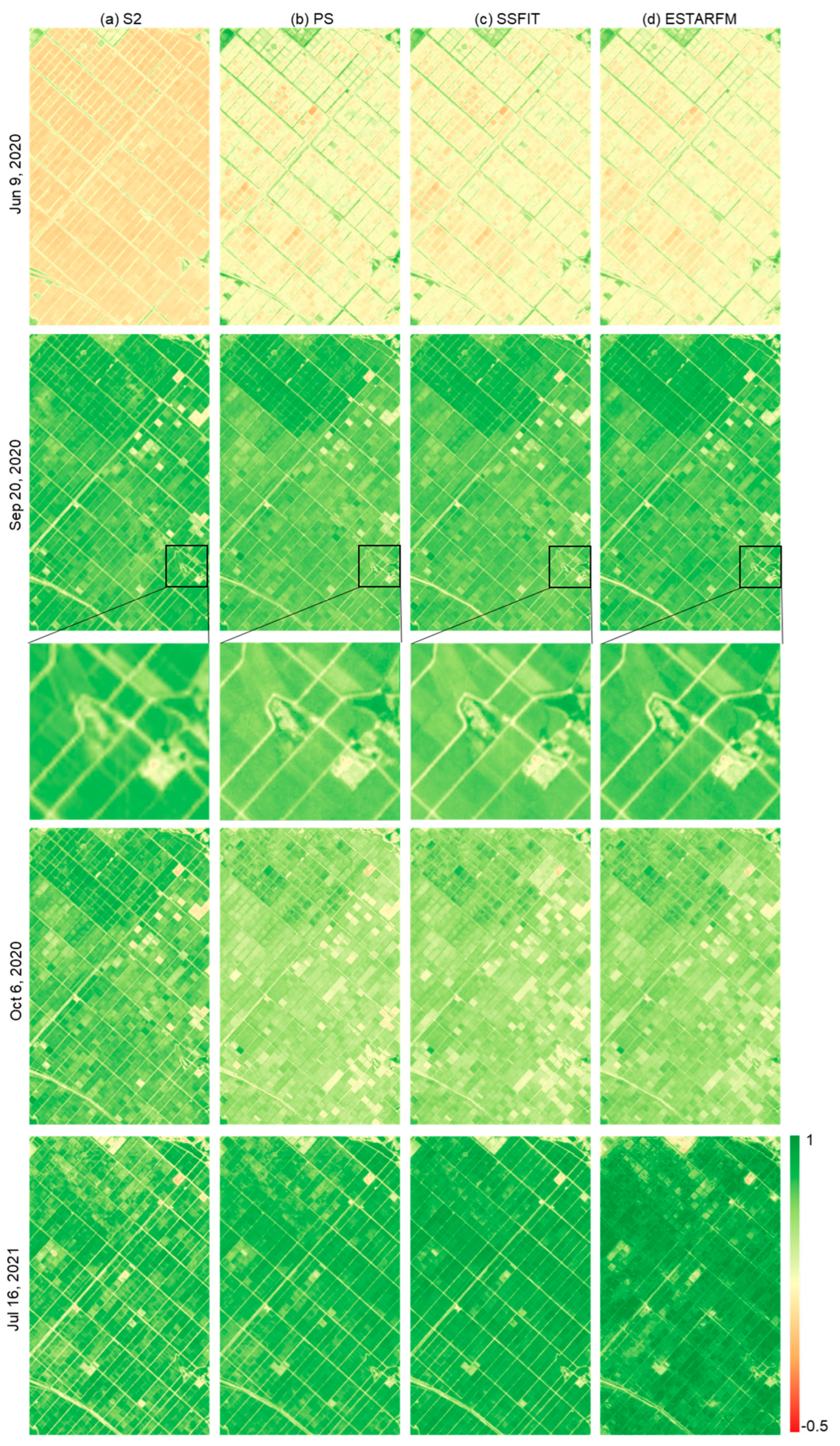
Figure 5.
NDVI images of the cabbage field area on the prediction dates from 2019 to 2021.
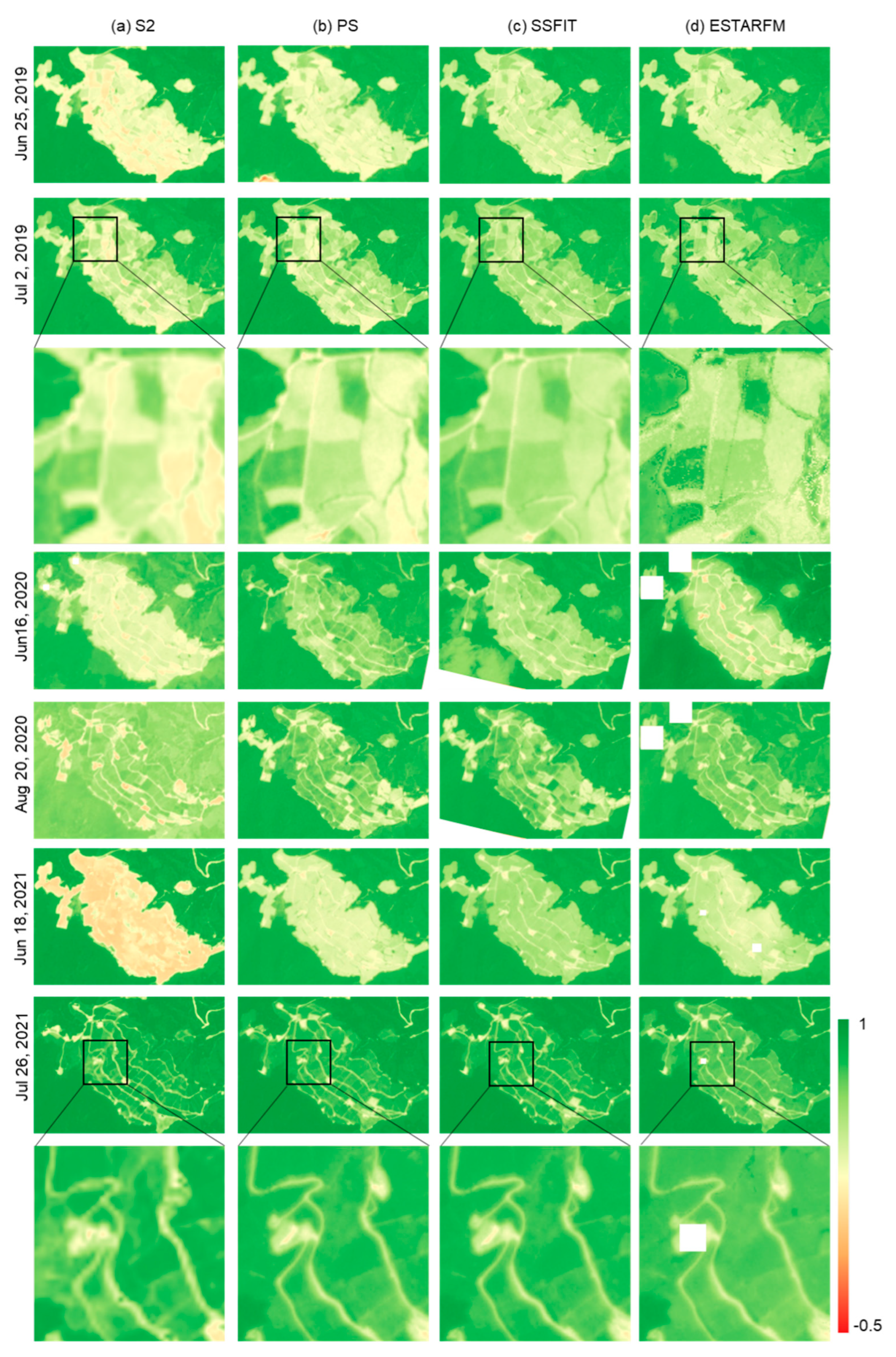
Figure 6.
Observed and predicted time-series NDVI patterns from 2019 to 2021: (a) rice paddy; (b) cabbage field.
Figure 6.
Observed and predicted time-series NDVI patterns from 2019 to 2021: (a) rice paddy; (b) cabbage field.
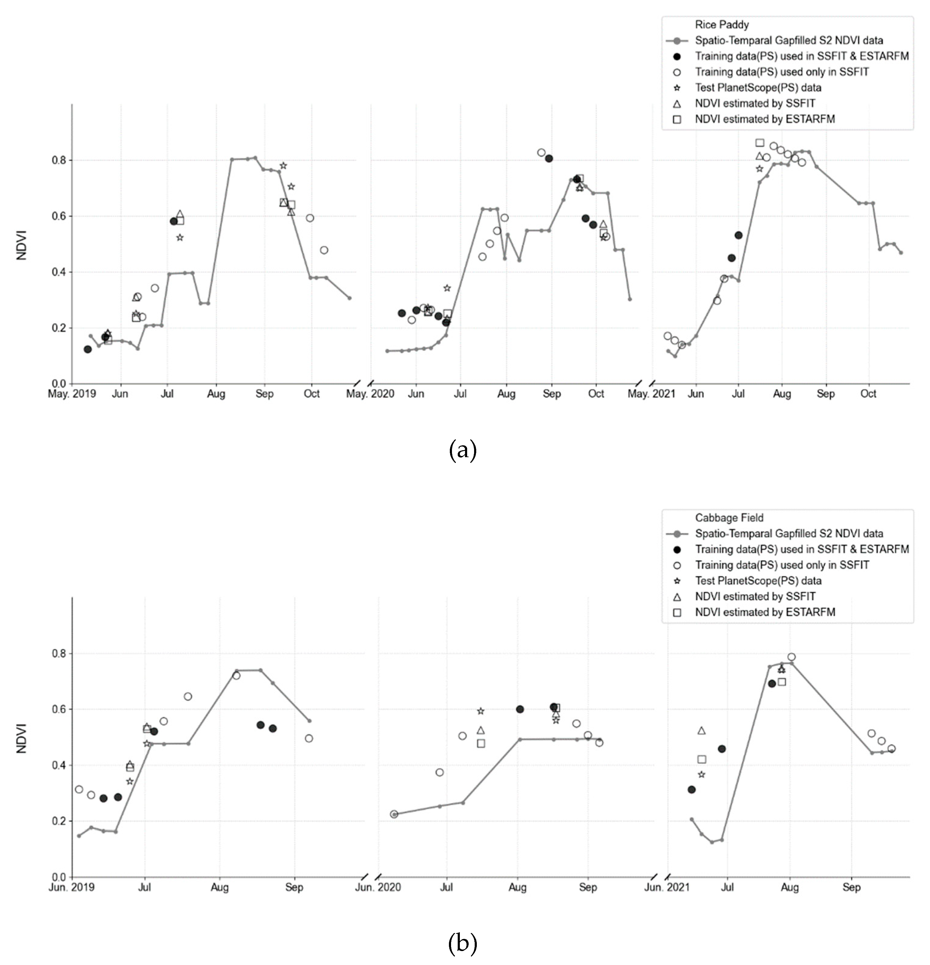
Figure 7.
Scatter plots of STF NDVI and PS test NDVI for the rice paddy on September 20, 2020: (a) SSFIT; (b) ESTARFM.
Figure 7.
Scatter plots of STF NDVI and PS test NDVI for the rice paddy on September 20, 2020: (a) SSFIT; (b) ESTARFM.
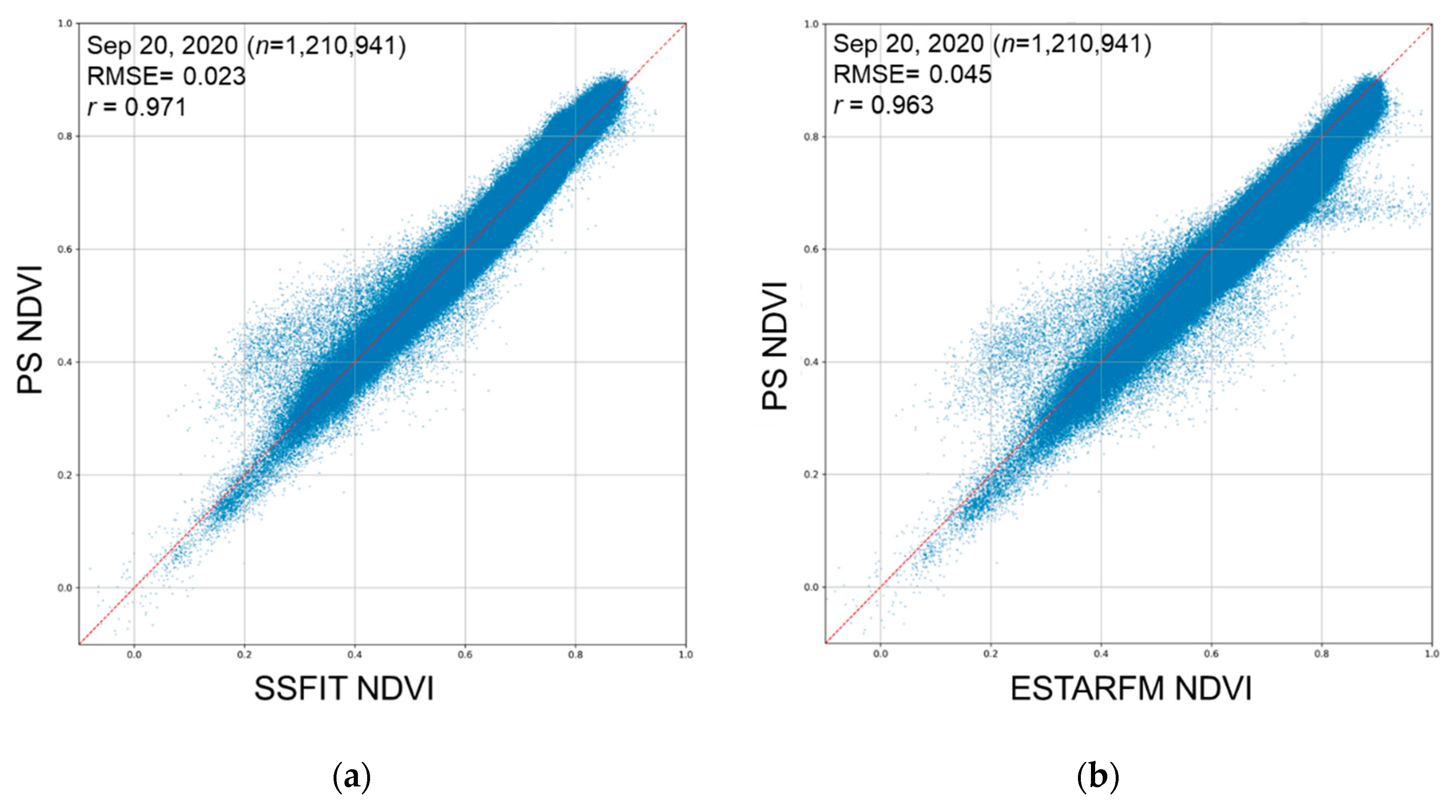

Table 1.
Specifications of two study areas and dataset used.
| Site | Rice paddy | Highland cabbage field |
|---|---|---|
| Location (Area) |
37.03071°N, 126.50696°E (1,042.5 ha) |
37.21837°N, 128.96659°E (102.6 ha) |
| Growing period of crops | The fields are filled with water in April, rice seedlings are planted in May, and harvested in October |
Sowing takes place from May to June, and harvesting takes place from August to September. The sowing period, growing status, and harvesting period vary depending on the plot |
| S2 L2A (10m, 5 days) |
From May 13~Oct 25, 2019 (24 scenes) From May 12~Oct 24, 2020 (26 scenes) From May 12~Oct 24 2021 (25 scenes) |
From Jun 4~Sep 7, 2019 (11 scenes) From Jun 8~Sep 6, 2020 (8 scenes) From Jun 13~Sep 21, 2021 (10 scenes) |
| PS Dove L3B (3m, occasional) |
From May 11~Oct 9, 2019 (13 scenes) From Apr 29~Oct 6, 2020 (21 scenes) From May 12~Aug 15, 2021 (14 scenes) |
From Jun 4~Sep 7, 2019 (14 scenes) From Jun 8~Sep 6, 2020 (10 scenes) From Jun 13~Sep 21, 2021 ( 9 scenes) |
Table 2.
Accuracy of STF NDVI image estimated based on PS test NDVI image in the rice paddy.
| Date | RMSE (r) of SSFIT | RMSE (r) of ESTARFM | |
|---|---|---|---|
| 2019 | May 24 Jun 11 Jul 9 Sep 13 Sep 18 |
0.068 (0.860) 0.096 (0.840) 0.151 (0.851) 0.139 (0.828) 0.110 (0.801) |
0.073 (0.849) 0.078 (0.837) 0.158 (0.833) 0.140 (0.793) 0.102 (0.693) |
|
2020 |
Jun 9 Jun 22 Sep 20 Oct 6 |
0.024 (0.994) 0.125 (0.893) 0.023 (0.971) 0.046 (0.914) |
0.029 (0.979) 0.107 (0.909) 0.045 (0.963) 0.062 (0.932) |
| 2021 | Jul 16 | 0.057 (0.951) | 0.131 (0.723) |
Table 3.
Accuracy of STF NDVI image estimated based on PS test NDVI image in the cabbage fields.
| Date | RMSE (r) of SSFIT | RMSE (r) of ESTARFM | |
|---|---|---|---|
| 2019 | Jun 25 Jul 2 |
0.073 (0.969) 0.056 (0.988) |
0.069 (0.966) 0.089 (0.944) |
|
2020 |
Jun 16 Aug 20 |
0.084 (0.883) 0.049 (0.971) |
0.134 (0.874) 0.064 (0.943) |
|
2021 |
Jun 18 Jul 28 |
0.104 (0.980) 0.004 (0.999) |
0.048 (0.989) 0.032 (0.984) |
Disclaimer/Publisher’s Note: The statements, opinions and data contained in all publications are solely those of the individual author(s) and contributor(s) and not of MDPI and/or the editor(s). MDPI and/or the editor(s) disclaim responsibility for any injury to people or property resulting from any ideas, methods, instructions or products referred to in the content. |
© 2025 by the authors. Licensee MDPI, Basel, Switzerland. This article is an open access article distributed under the terms and conditions of the Creative Commons Attribution (CC BY) license (http://creativecommons.org/licenses/by/4.0/).
Copyright: This open access article is published under a Creative Commons CC BY 4.0 license, which permit the free download, distribution, and reuse, provided that the author and preprint are cited in any reuse.


