Submitted:
14 January 2026
Posted:
14 January 2026
You are already at the latest version
Abstract
Rapid economic growth does not necessarily translate into better perceived urban health. Using the 2024 nationwide Urban Physical Examination (UPE) resident survey in China, this study assesses how city economic level relates to perceived urban health, proxied by city-level overall satisfaction. The survey was conducted in April–June 2024 in the main urban districts of 47 cities, yielding 692,800 responses and 499,500 valid questionnaires. We aggregate satisfaction to the city level, match it with GDP and key city characteristics, and estimate the GDP–satisfaction association using restricted cubic splines (RCS) to test for potential non-linearity. Across unadjusted and covariate-adjusted models (accounting for population scale and density, industrial structure, fiscal capacity, and regional effects), results show a robust positive association between economic level and satisfaction, while nested-model tests provide no evidence that spline terms improve fit over a linear specification within the observed GDP range. Substantial dispersion around the fitted curve indicates that GDP is an enabling capacity rather than a sufficient condition, pointing to cross-city differences in how effectively resources are converted into lived urban quality. We propose using GDP-adjusted satisfaction benchmarking within the UPE cycle to identify underperforming cities and prioritize targeted governance and renewal actions.
Keywords:
urban physical examination (UPE)
; perceived urban health
; city satisfaction
; GDP
; restricted cubic splines
; China
; benchmarking
1. Introduction
China has entered a phase of high urbanization in which rapid economic expansion coexists with persistent “urban maladies”. By the end of 2023, the urbanization rate of permanent residents reached 66.16%, indicating a predominantly urban society(Organizational Chart, 2022). Yet, high GDP does not necessarily translate into a “healthy city” in residents’daily experience: even economically advanced cities may face severe congestion, recurrent pluvial flooding, public safety concerns, and environmental degradation, while some less affluent cities may offer more affordable housing, more manageable commuting burdens, and better everyday accessibility(Connor et al., 2025). In response, China has promoted the Urban Physical Examination (UPE) as a problem-oriented governance instrument since 2018, with pilots launched in 11 cities in 2019 and subsequent expansion(Liu & Fang, 2025; Zhang et al., 2021). A distinctive feature of UPE is the institutionalization of large-scale resident surveys, where city-level satisfaction serves as a key people-centred indicator to assess perceived “urban health” alongside objective diagnostics(Pazos-García et al., 2025; Shi et al., 2021). Therefore, it is an important initiative that can effectively reflect the health of the city.
From an academic standpoint, the link between economic development and perceived urban health is theoretically non-linear and empirically debated. Subjective well-being (SWB) research generally finds that income is positively associated with evaluative measures (e.g., life satisfaction), but the marginal returns may diminish due to adaptation and social comparison(Kahneman & Deaton, 2010; Killingsworth, 2021; Roszkowska et al., 2025). Cross-country evidence, however, often reports a robust positive association between national income and average SWB, suggesting that the growth–well-being relationship can be context-dependent rather than universally plateauing. These debates imply that the GDP–satisfaction relationship may exhibit threshold, plateau, or other non-linear patterns—functional forms that are substantively important for policy interpretation(Killingsworth et al., 2023). Meanwhile, urban perceived health/quality of life (QoL) is multidimensional and shaped by demographic pressure, the built environment, public service provision, and environmental management—domains emphasized in the “healthy city” paradigm(He et al., 2024; Nicolás-Martínez et al., 2024a). In the UPE context, these domains also tend to covary with economic level; therefore, empirical models that relate GDP to resident-rated city satisfaction should, at minimum, account for key city characteristics (e.g., population, density, industrial structure, fiscal capacity) to reduce omitted-variable bias(Yu et al., 2024). Methodologically, restricted cubic splines (RCS) provide a flexible and interpretable approach to diagnosing and testing non-linearity without imposing arbitrary cut-points(Desquilbet & Mariotti, 2010).
Against this background, this study examines whether and how city economic level (GDP) is associated with city-level overall satisfaction—used as a parsimonious proxy for perceived urban health—using the 2024 nationwide UPE resident survey dataset (details reported in the Data section). We estimate both a linear benchmark model and an RCS specification, and formally test non-linearity via nested-model comparisons, in both unadjusted and covariate-adjusted settings (Figure 1). The analysis is organized around two core expectations: H1: higher GDP is associated with higher city-level satisfaction; H2: the GDP–satisfaction association is non-linear, consistent with diminishing marginal returns or threshold/plateau patterns suggested by SWB theory. By clarifying the functional form of the GDP–perceived urban health relationship under an institutionalized people-centred governance framework (UPE), the study provides evidence for differentiated policy interpretation beyond “more growth is always better”(Jebb et al., 2018).
2. Data and Methods
2.1. Data Sources
This study draws on the nationwide Urban Physical Examination (UPE) resident survey organized by the Ministry of Housing and Urban-Rural Development (MoHURD) in 2024. The questionnaire was designed to capture residents’ perceived urban conditions across four spatial scales—dwelling, neighborhood/community, block, and city—and operationalized through 45 indicators spanning eight domains (e.g., safety and durability, ecological livability, safety resilience, and jobs–housing balance). The survey was implemented between April and June 2024 within the main urban districts of the sampled cities. In total, 692,800 questionnaires were collected from 47 cities; after data cleaning, 499,500 valid responses were retained, yielding an effective response rate of 71.96%.
The target population comprised local permanent residents aged 16 years and above who had resided in the city for at least six months, excluding short-term visitors and transient workers with shorter stays. To enhance representativeness and comparability across cities, the fieldwork adopted multiple sampling and quota-control strategies, including proportional stratified sampling and cross-quota controls, to ensure broad and balanced coverage in respondents’ spatial distribution and socio-demographic structure (gender, age, occupation, and income).
The 47-city sample was selected to reflect heterogeneity in economic level, population scale, and geographical location, enabling cross-city comparison across diverse development contexts. This rationale is visualized in the national overview figure (Figure 2), which maps the sample cities and highlights between-city variation in GDP and population size. In the empirical analysis, individual responses are aggregated to the city level to construct the study outcome (overall satisfaction as a proxy for perceived urban health), while GDP and other city characteristics are matched at the same administrative level. Descriptive statistics of all study variables are reported in Table 1.
2.2. Methods and Preprocessing
- (1)
- Data preprocessing and analytic sample
The MoHURD UPE microdata were first screened according to the survey’s eligibility criteria (permanent residents aged ≥16 years with a minimum six-month residence). We then aggregated individual responses to the city level to construct the dependent variable, overall city satisfaction (Satisfaction), using the arithmetic mean of valid responses within each city. City-level socioeconomic covariates were harmonized to the same administrative level and matched to the 47 sampled cities. Given the strong right-skewness typical of macroeconomic indicators, GDP was log-transformed (log(GDP)) prior to modeling. Control variables were transformed when appropriate (e.g., logarithmic transformation for population and fiscal expenditure per capita) to reduce skewness and to improve linearity in covariate–outcome relations. In addition, to ensure model stability, we diagnosed collinearity among candidate covariates (pairwise correlations and VIF) and retained the final set of covariates used in the adjusted models.
- (2)
- Restricted cubic splines for non-linear GDP–satisfaction associations
To characterize potential non-linear associations between economic level and perceived urban health, we modeled log(GDP) using restricted cubic splines (RCS) (also referred to as natural cubic splines)(Austin, 2025; Gauthier et al., 2020). RCS offers a flexible yet parsimonious functional form: it allows curvature within the data range while constraining the relationship to be linear in the tails, reducing implausible extrapolation(Discacciati et al., 2025).
Let denote the city-level satisfaction score for city , denote , and denote a vector of city-level covariates. The RCS regression can be written as:
where is approximated by an RCS basis expansion:
with knots , and . A commonly used restricted basis is:
In practice, spline complexity can be parameterized either by the number of knots or by the degrees of freedom (df) of the spline basis. Consistent with best practices for small-to-moderate samples, we adopted an RCS specification with df = 4 for the main analysis and evaluated robustness using alternative df settings (df = 3 and df = 5) to ensure that substantive conclusions were not driven by overfitting or underfitting. The df choice reflects a standard trade-off: sufficient flexibility to capture plausible curvature while maintaining interpretability and statistical power given the city-level sample size(Arnes et al., 2023; Discacciati et al., 2025).
- (3)
- Model specification: unadjusted vs adjusted
We estimated two nested specifications, each under both linear and RCS functional forms for :
(a) Unadjusted model
where is either a linear term () or the RCS function .
(b) Adjusted model
where includes city demographic and structural characteristics (e.g., population size, population density, industrial structure, fiscal capacity) and broad regional indicators to account for spatially clustered heterogeneity.
- (4)
- Inference on non-linearity: nested-model F test
To formally assess whether the GDP–satisfaction association departs from linearity, we conducted a nested-model F test comparing the RCS model (full) against the linear model (restricted)(Schuster et al., 2022). The null hypothesis is that all spline terms beyond the linear component jointly equal zero:
Let and denote residual sums of squares from the linear and RCS models, respectively; let be the number of additional spline parameters beyond linearity; and let be the number of parameters in the full model (including the intercept). The test statistic is:
which follows an distribution under . We applied this procedure to both the unadjusted and adjusted specifications, thereby testing non-linearity conditional on covariates.
- (5)
- Reporting and visualization
For interpretability, we report model-predicted satisfaction across the observed range of log(GDP) and visualize the fitted RCS curve with 95% confidence intervals (CI). In addition to the spline plots, we present scatterplots of GDP versus satisfaction with an overlaid trend line to convey the raw association prior to functional-form modeling.
3. Results
3.1. Descriptive AssociationBbetween GDP anC ciLy-leSel Satisfaction
Figure 3 presents the bivariate relationship between GDP and city-level overall satisfaction (city-aggregated UPE score) across 47 sampled cities. The scatterplot indicates a moderate positive association: cities with higher GDP tend to report higher average satisfaction, although the dispersion is substantial, suggesting that economic level alone does not fully explain perceived urban health.
The OLS fitted trend line corroborates this pattern. Using GDP as a continuous predictor, the association is statistically positive (Pearson r = 0.41; R² = 0.17; slope p = 0.004). At the same time, the 95% CI widens toward the upper tail of GDP, consistent with fewer high-GDP observations and greater uncertainty in that range. Notably, several mid- and low-GDP cities achieve satisfaction levels comparable to (or exceeding) some higher-GDP cities, implying meaningful heterogeneity associated with non-economic city attributes (e.g., urban management, service provision, and environmental conditions).
3.2. Covariate Screening and CcollinearitD Diagnostics
To ensure that the subsequent multivariable (linear and RCS) estimates are not distorted by redundant predictors, we conducted a structured collinearity diagnosis prior to model estimation. Specifically, we examined (i) the pairwise Pearson correlation structure of candidate variables and (ii) variance inflation factors (VIFs) for the covariate set intended for inclusion in adjusted models. This step is necessary in a city-level design, where macro indicators (e.g., economic scale, population scale, fiscal capacity, and service provision) can be strongly interrelated, potentially inflating standard errors and obscuring substantive interpretation.
The correlation matrix for the broader pool of city-level indicators, including UPE domain-level indices and auxiliary socioeconomic/service indicators is shown in Figure 4. Two patterns are particularly notable. First, overall satisfaction is highly correlated with several UPE domain indices those sub-level dimensions we set in the questionnaire (e.g., ecological livability, safety resilience, jobs–housing balance), with correlations typically above 0.89 (and up to ≈0.96 in the strongest pairs). This coherence indicates that the domain indices capture closely related latent perceptions; accordingly, we do not treat these domain indices as exogenous controls in the GDP–satisfaction model to avoid mechanical overlap/over-adjustment (i.e., controlling for components of the outcome). Second, a “scale-and-capacity” cluster emerges among macro indicators—GDP, fiscal expenditure, population, and healthcare capacity measures (e.g., hospitals and beds)—with several pairs exhibiting correlations above 0.80 (e.g., GDP vs fiscal expenditure ≈ 0.93; beds vs hospitals ≈ 0.94). This pattern suggests that raw-size indicators contain substantial shared variance and should not be simultaneously included in their original forms.
Figure 5 narrows the focus to the covariate candidates intended for econometric modeling after harmonization and transformation: log(GDP), log(population), population density, tertiary-industry share, log(fiscal expenditure per capita), and three service/environment indicators (beds per 10,000 persons, wastewater treatment rate, harmless domestic waste treatment rate). Within this set, the strongest association is observed between log(GDP) and log(population) (r ≈ 0.83), followed by log(GDP) and population density (r ≈ 0.69). The remaining correlations are moderate (generally ≤ 0.52), indicating that most covariates provide non-redundant information once variables are expressed in per-capita terms or log-transformed where appropriate. Therefore, we used the 8 indicators shown in Figure 5.
To further ensure that there is no collinearity between the variables used in the end, we further use VIF diagnostics. Table 2 reports VIF and tolerance values for the model-candidate covariate set. The largest VIFs correspond to log(GDP) (VIF = 7.48) and log(population) (VIF = 6.70), consistent with the high pairwise correlation noted above. Importantly, these values remain below the conventional threshold for severe multicollinearity (VIF > 10), while other predictors exhibit low-to-moderate VIFs (1.19–2.64), suggesting limited collinearity concerns for the remaining covariates. Together, the correlation heatmaps and VIF results indicate that multicollinearity is manageable and primarily concentrated in the expected overlap between economic scale and population scale.
Final covariate choice for adjusted models. Balancing statistical stability with parsimony in a city-level sample, the baseline adjusted specification retains a core set of controls that capture demographic pressure and structural capacity: log(population), population density, tertiary-industry share, and log(fiscal expenditure per capita), along with broad regional indicators (to absorb spatially clustered heterogeneity). The three service/environment indicators are retained as analytically meaningful descriptors and can be used in extended specifications/sensitivity checks; however, the main adjusted results emphasize the parsimonious control set to preserve degrees of freedom and minimize redundancy.
This covariate-screening procedure provides a transparent foundation for the subsequent estimation of the GDP–satisfaction relationship, including formal tests of non-linearity under the RCS framework.
3.3. Non-LinearRrelationshiA Assessment
(1) Model construction
Building on the descriptive pattern reported in and the covariate screening above, we next focus on the functional form of the economic–perceived urban health association. Figure 6a plots raw GDP against city-level overall satisfaction. Two features are salient. First, GDP is highly right-skewed, with most observations concentrated at the lower end and a small number of very high-GDP cities forming a long upper tail. This uneven distribution implies that a linear fit in the raw scale may be disproportionately influenced by a few high-GDP observations. Second, the dispersion of satisfaction is sizable across the GDP range, indicating that economic scale alone is insufficient to account for perceived urban health.
To improve scale comparability and mitigate skewness, Figure 6b re-expresses the predictor as log(GDP). After transformation, observations are more evenly distributed along the x-axis, and the GDP–satisfaction gradient becomes easier to interpret. Importantly, visual inspection suggests possible departures from strict linearity, particularly at the lower end of log(GDP) where the fitted relation appears slightly curved rather than strictly monotonic. This motivates the use of a flexible functional form that can capture smooth curvature while avoiding arbitrary stratification. This phenomenon is usually considered to be a nonlinear relationship between variables.
Accordingly, we adopted restricted cubic splines (RCS) for log(GDP). A key modeling decision is the spline complexity, commonly parameterized by the degrees of freedom (df). Figure 7 compares RCS fits under df = 3, 4, and 5. The three specifications yield a consistent overall pattern—an increasing association between log(GDP) and satisfaction—while differing in smoothness. The df = 3 model produces the smoothest curve and largely approximates a near-linear trend; df = 5 introduces more local curvature (i.e., greater sensitivity to small-sample fluctuations, especially near the tails); and df = 4 provides a middle-ground specification that allows moderate curvature without overfitting. Based on this sensitivity check and the city-level sample size, df = 4 was selected as the main specification, with df = 3 and df = 5 retained as robustness alternatives.
3.3.2. RCS Estimates of the GDP–satisfactionRrelationship
Using the selected spline specification (RCS with df = 4), we estimated the GDP–satisfaction association under two nested model settings: an unadjusted model including only , and an adjusted model controlling for city characteristics (population scale and density, industrial structure, fiscal capacity, and region indicators).
(1) Unadjusted RCS
The unadjusted RCS curve indicates a positive, largely monotonic association between and city-level satisfaction (Figure 8). The fitted line rises gradually across the observed range, with slightly stronger gains toward the upper tail, while the 95% CI expands at both ends, reflecting greater uncertainty where observations are sparse. In terms of magnitude, predicted satisfaction increases from 73.19 (95% CI: 71.71–74.67) at the 10th percentile of to 77.37 (95% CI: 75.78–78.96) at the 90th percentile—an absolute difference of approximately 4.18 points (holding other terms absent in this model). Consistent with the segmented visualization, the GDP distribution can be partitioned into three ranges using the two vertical cut-points (Stage A/B/C) at and (corresponding to GDP and in the original scale), within which the curve remains smooth and upward-sloping rather than exhibiting abrupt jumps.
(2) Adjusted RCS
After adjustment for the screened covariates, the overall shape remains qualitatively unchanged: satisfaction still increases with , and the curve remains smooth without pronounced inflection (Figure 9). However, the adjusted model explains a substantially larger share of cross-city variation (R² = 0.41; Adj. R² = 0.23) than the unadjusted model (R² = 0.20; Adj. R² = 0.14), indicating that non-economic city attributes jointly account for meaningful heterogeneity in perceived urban health. Predicted satisfaction rises from 70.51 (95% CI: 66.71–74.31) at the 10th percentile of to 78.16 (95% CI: 73.33–83.00) at the 90th percentile, corresponding to an approximate increase of 7.65 points (evaluated at the covariate baseline used for prediction). The segmented cut-points are highly consistent with the unadjusted model ( and ; GDP and ), again suggesting gradual rather than discontinuous changes across the economic spectrum.
(3) Formal non-linearity tests
Despite the visual flexibility of the spline, the nested-model F tests comparing the linear specification against the RCS specification provide no statistical evidence of non-linearity in either setting (Table 3): unadjusted ; adjusted . Taken together, these results indicate that the GDP–satisfaction association is robustly positive, while any curvature implied by the fitted spline is weak and not statistically distinguishable from a linear trend given the current city-level sample.
3.3.3. Robustness and Specification Ssensitivity
To assess whether the substantive conclusions depend on modeling choices rather than the underlying data pattern, we conducted a set of specification and sensitivity checks focusing on (i) the scale of the economic indicator, (ii) spline flexibility, and (iii) potential instability at the distribution tails.
(1) Scale transformation (GDP vs. log(GDP))
Because city GDP is markedly right-skewed, modeling GDP on the raw scale may overweight a small number of high-GDP cities and obscure the central tendency in the majority of observations. The log transformation improves leverage balance and yields a more interpretable gradient across the economic spectrum. Consistent with the visual comparison in Section 3.3.1, the positive GDP–satisfaction association is preserved after transformation, while the log scale provides a more stable basis for functional-form assessment.
(2) Spline complexity (df sensitivity)
We re-estimated spline models using alternative degrees of freedom (df = 3 and df = 5) to evaluate the robustness of the inferred curve shape. Across these alternatives, the fitted RCS functions remained qualitatively consistent: the association between log(GDP) and satisfaction is generally increasing, and any curvature is modest. The df = 3 model produced a smoother, near-linear trajectory, whereas df = 5 allowed more local fluctuations, particularly near the tails where observations are sparse and uncertainty is inherently higher. These comparisons support df = 4 as a parsimonious main specification that balances flexibility and stability, while indicating that the key inference—an overall positive association with weak curvature—does not hinge on a specific df setting.
(3) Tail uncertainty and influence considerations.
Across unadjusted and adjusted RCS plots, confidence intervals widen toward both ends of the log(GDP) distribution, reflecting reduced information at the extremes. This pattern underscores that fine-grained interpretation of slope changes at the lowest or highest GDP ranges should be treated cautiously. Importantly, however, the formal nested-model tests show that introducing spline terms does not yield a statistically detectable improvement over a linear specification (Section 3.3.2), indicating that any apparent tail curvature is not sufficiently supported by the available city-level sample.
(4) Implication for subsequent reporting.
Taken together, the sensitivity checks suggest that (i) the positive GDP–satisfaction relationship is robust to reasonable transformations and spline parameterizations, and (ii) the evidence for non-linearity is weak. Accordingly, we retain the RCS specification primarily as a transparent visualization tool for the functional form, while using the linear model as the benchmark for parsimonious inference and interpretation.

Table 4.
Robustness and specification sensitivity checks.
| Robustness check | Alternative specification(s) | Purpose | Key finding | Implication |
|---|---|---|---|---|
| Scale transformation | GDP (raw) vs. log(GDP) | Reduce right-skewness and leverage of extreme GDP values; improve interpretability. | Positive association persists after log transformation; log scale yields a more even spread of cities across the x-axis. | Use log(GDP) in all regression models. |
| Spline flexibility (df) | RCS df = 3, 4, 5 | Assess sensitivity of curve shape to spline complexity (under-/over-fitting). | Overall increasing pattern is stable across df; df=5 shows more tail fluctuation; df=3 approximates near-linearity; df=4 balances flexibility and stability. | Adopt df=4 as main specification; report df=3 and df=5 as sensitivity. |
| Formal non-linearity test | Nested F-test: Linear vs RCS (df=4) | Test whether spline terms add explanatory power beyond linearity. | Unadjusted: F=0.21, p=0.811 (N=47); Adjusted: F=0.08, p=0.919 (N=45). | Non-linearity is not statistically supported; linear model remains a parsimonious benchmark. |
| Tail uncertainty | Inspect 95% CI width along log(GDP) | Evaluate stability where observations are sparse (distribution tails). | CI widens at low and high log(GDP), indicating higher uncertainty at distribution tails. | Avoid over-interpreting local curvature at extremes; emphasize overall trend. |
Note: This table summarizes the specification checks reported in Section 3.3.3. RCS main specification uses df=4. RCS model fit (df=4): unadjusted R²=0.199 (Adj. R²=0.143); adjusted R²=0.406 (Adj. R²=0.232).
4. Discussion
4.1. Main Findings and Iinterpretation oC curSe Shape
This study provides a city-level assessment of how economic capacity (GDP) is associated with perceived urban health, proxied by UPE-based overall satisfaction aggregated to the city level. Across both the descriptive bivariate evidence and the regression-based specifications, the central empirical result is consistent: cities with higher GDP tend to report higher overall satisfaction, but the relationship is far from deterministic, as indicated by substantial between-city dispersion around the fitted trend.
(1) “No plateau within the observed range”: GDP as an enabling capacity for urban health.The near-linear increasing profile can be read as evidence that, for the sampled cities, additional economic capacity continues to translate into improvements in domains that residents experience directly and evaluate positively—such as infrastructure maintenance, public service coverage, environmental management capacity, and the city’s ability to respond to risks and disruptions. Under the UPE framework, overall satisfaction is a comprehensive, people-centred outcome that plausibly reflects the cumulative performance of these systems. If economic resources are effectively converted into public goods and urban management quality, then a plateau is not inevitable; rather, “economic upgrading” may continue to yield observable gains in perceived urban health.
(2) “Diminishing returns may exist but are difficult to detect at city level”: bounded outcomes and offsetting externalities. The absence of statistically detectable curvature does not rule out diminishing marginal returns in principle. Satisfaction is a bounded, composite perception; as baseline conditions improve, incremental gains become harder to achieve and to measure. Moreover, higher-GDP cities frequently face countervailing pressures—congestion, housing cost burdens, environmental externalities, and governance complexity—that can partially offset the benefits of economic affluence. Empirically, this tension is visible in two ways: (i) the fitted curve’s confidence band expands toward the distribution tails (especially at high ), indicating greater uncertainty where observations are sparse; and (ii) cities with similar GDP can differ markedly in satisfaction, suggesting that the conversion efficiency from economic resources to lived urban quality varies widely. In short, a “plateau story” may be conceptually plausible, but the current cross-sectional city-level design—particularly with limited density in the extreme GDP ranges—may be underpowered to distinguish subtle curvature from noise.
(3) The most policy-relevant reading of these findings is therefore not “GDP matters” per se, but what GDP represents and what it does not. GDP appears to operate as a resource base that is generally associated with higher perceived urban health; however, the large dispersion around the curve indicates that GDP is necessary but not sufficient. Some cities achieve relatively high satisfaction at modest GDP levels (suggesting strengths in governance, service delivery, or urban form), while others underperform relative to their GDP (suggesting that negative externalities or misallocation may dominate residents’ daily experience). This “overperformer/underperformer” pattern is precisely why a flexible functional-form assessment is valuable: it frames GDP as an enabling condition, while directing analytical and policy attention toward the factors that shape how economic capacity is translated into resident-perceived urban health.
4.2. Comparison with Prior Lliterature
Our findings contribute to, and partially reconcile, several established but sometimes divergent strands of research on the economy–well-being nexus.
First, the direction and overall monotonicity of the GDP–satisfaction relationship aligns with the dominant “positive gradient” view in macro-level well-being research(Oishi et al., 2022; Prati, 2024). Cross-country and long-run evidence generally indicates that higher average economic development is associated with higher average subjective well-being, and some influential re-analyses argue against a clear “satiation point” at the national level(Nicolás-Martínez et al., 2024b). Consistent with this perspective, our city-level results show a robust positive association between economic capacity and residents’ overall evaluation of their city, and the flexible RCS specification does not yield statistically detectable curvature relative to a linear benchmark(Killingsworth, 2021; Killingsworth et al., 2023).
Second, our results differ in emphasis from the “income satiation / diminishing returns” literature that is largely grounded in individual-level data. Studies distinguishing evaluative well-being from experienced affect have reported plateau-like patterns for some components of well-being (e.g., emotional well-being) beyond a threshold income, while other work identifies turning points and region-specific satiation levels(Killingsworth, 2021; Killingsworth et al., 2023). In contrast, we do not observe a statistically identifiable plateau within the GDP range covered by the 47-city sample. This discrepancy is not necessarily contradictory: (i) our outcome—city-level overall satisfaction—is closer to an evaluative judgment (how residents appraise their city as a whole) than to momentary affect, and evaluative measures are commonly found to scale more linearly with economic resources; (ii) we use city GDP (scale capacity) rather than household income, and the mapping from aggregate resources to individual experience depends on how effectively cities convert fiscal and economic capacity into public goods and everyday urban functioning(Xu et al., 2024).
Third, relative to urban quality-of-life (QoL) and “unhappy cities” scholarship, our evidence underscores the non-sufficiency of economic prosperity and highlights the role of urban externalities and governance capacity in explaining cross-city heterogeneity(Carlsen & Leknes, 2022). In the cities literature, QoL is often conceptualized as multidimensional, where economic performance is only one component among services, environment, safety, housing, mobility, and social cohesion; consequently, GDP per capita tends to be positively associated with life satisfaction, but it does not fully account for the spatial distribution of well-being(Carlsen & Leknes, 2022; Nicolás-Martínez et al., 2024b; Węziak-Białowolska, 2016). Related urban-economics arguments emphasize that large, prosperous cities can simultaneously generate disamenities (e.g., congestion, high costs, stressors) that offset gains in average well-being, producing substantial dispersion even at similar levels of development(Glaeser et al., 2016). Our results mirror this core insight: the scatter around the fitted GDP–satisfaction curve is substantial, and after adjustment the model fit improves (higher R²), implying that non-economic city attributes systematically structure perceived urban health beyond GDP alone(Sørensen, 2024).
Fourth, compared with China-focused evidence, our findings are consistent with the view that urban well-being in China is jointly shaped by structural urbanization conditions and city-level governance/service performance(Guo et al., 2025; Liao et al., 2022a). Research on life satisfaction in urbanizing China highlights the importance of city context (e.g., city size and institutional conditions) for residents’ evaluations(Chen et al., 2015). Complementary applied studies in the Chinese context suggest that resilience, management, and service provision are salient correlates of subjective well-being and satisfaction, reinforcing the interpretation that “conversion efficiency” from resources to lived experience matters(Liao et al., 2022b). Importantly, this resonates with the institutional design of China’s Urban Physical Examination (UPE) practice, which explicitly treats residents’ satisfaction as a core output alongside objective performance metrics and action lists—thereby embedding subjective evaluation into urban governance cycles(Liao et al., 2022b).
4.3. Policy Implications
Differentiated strategies by GDP range remain essential because constraints and marginal returns differ by development stage, even if the overall association is monotonic. For lower-GDP cities, the highest-yield interventions typically concentrate on basic-function reliability—maintenance of aging infrastructure, drainage and flood control, neighborhood safety and lighting, last-mile accessibility, and visible micro-environment upgrades that quickly reduce daily friction. In these contexts, resident satisfaction often responds strongly to improvements that stabilize core services and reduce recurrent disruptions, and the governance priority is to build credible, measurable delivery capacity rather than pursuing broad, capital-intensive expansion.
For middle-GDP cities, the policy frontier shifts from “coverage” to system integration and quality upgrading. Rapid spatial expansion, motorization, and rising expectations mean that residents increasingly evaluate the city through time-cost and convenience: commuting reliability, congestion management, facility accessibility, and the perceived fairness of service distribution. Here, simply increasing investment is rarely sufficient; what matters is coordination across land use–transport–public services–environment, to avoid fragmented projects that raise costs without improving lived experience. In practice, UPE results can be used to identify whether dissatisfaction clusters around jobs–housing balance, mobility, ecological livability, or safety resilience, and then to implement integrated packages rather than single-sector fixes.
For higher-GDP cities, the binding constraints tend to be externalities, cost pressures, and governance complexity. High GDP can coexist with persistent dissatisfaction if congestion, housing burdens, environmental exposure hotspots, or “fine-grained” neighborhood management deficits dominate residents’ daily experience. The implication is to prioritize externality control and governance modernization: demand management and multimodal transport reliability, affordability-oriented housing and rental governance, refined environmental exposure mitigation at the neighborhood scale, and responsive, data-driven urban management that closes the “last-mile governance gap.” In these cities, satisfaction gains are often achieved less by adding more infrastructure and more by improving operational performance and equity in service access.
Regional differentiation should be layered on top of GDP staging because “the same GDP” can imply different structural pressures. In coastal and high-density regions, satisfaction is often constrained by congestion, time-cost, high living expenses, and environmental exposure concentrated in dense neighborhoods; thus, policies should emphasize demand management, exposure hotspot governance, and equitable service reallocation. In inland or lower-density regions, accessibility coverage, basic public-service catchments, and infrastructure reliability frequently dominate perceived outcomes; thus, policies should emphasize service completion, maintenance regimes, and resilience of essential systems. For shrinking or slow-growth regions, the conversion-efficiency lens is particularly important: the priority is not expansion but right-sizing services, maintaining quality under fiscal constraints, and preventing “infrastructure decay” from eroding perceived urban health.
Finally, the results reinforce a governance shift: treat resident satisfaction not as a generic “soft indicator,” but as a performance metric that reveals where economic growth is not translating into lived benefits. The GDP–satisfaction curve can be institutionalized as a diagnostic tool within UPE practice—supporting differentiated renewal strategies, more accountable action lists, and a clearer focus on conversion efficiency. Over time, repeating the same analysis across survey waves would allow policymakers to evaluate whether cities are moving upward (raising satisfaction) and toward the benchmark (improving conversion), which is arguably the most actionable interpretation of “high-quality urban development” in a people-centred governance framework.
5. Conclusions
5.1. Summary
This study examined whether and how economic development (GDP) is associated with perceived urban health, proxied by city-level overall satisfaction aggregated from the 2024 nationwide Urban Physical Examination (UPE) resident survey. Using 47 Chinese cities, we first documented a moderate positive bivariate association between GDP and satisfaction, while also observing substantial cross-city dispersion—indicating that economic prosperity does not automatically translate into uniformly higher perceived urban health.
To move beyond a linear assumption, we employed restricted cubic splines (RCS) to flexibly assess the functional form of the GDP–satisfaction relationship. After log-transforming GDP to reduce skewness and leverage effects, the RCS estimates revealed a smooth, generally increasing association between log(GDP) and city-level satisfaction. However, nested-model tests comparing linear and spline specifications provided no statistical evidence of non-linearity in either the unadjusted model or the covariate-adjusted model. Together, these results suggest that, within the observed GDP range of the sampled cities, higher economic capacity is consistently associated with higher satisfaction, but the magnitude of perceived urban health is also strongly shaped by non-economic factors reflected in the dispersion around the fitted curve.
From a governance perspective, the findings support interpreting GDP as an enabling capacity rather than a sufficient condition. The observed heterogeneity implies that cities differ in their conversion efficiency—how effectively economic resources are translated into service quality, environmental conditions, mobility reliability, safety, and other everyday experiences that residents evaluate in the UPE system.
5.2. Future Work
Several limitations point to directions for future research and policy-oriented refinement.
First, the analysis is conducted at the city level; aggregating satisfaction to a single city mean inevitably masks within-city disparities. Future work should extend the framework to finer spatial units (e.g., districts or neighborhoods) to assess whether the economy–perceived urban health association differs across urban subareas and whether “conversion efficiency” varies within cities.
Second, the study uses a cross-sectional design. While the association between GDP and satisfaction is robust, causal interpretation remains limited. Longitudinal analyses using repeated UPE waves would allow testing whether changes in economic capacity and governance performance precede changes in resident satisfaction, and whether functional form evolves over time.
Third, although we controlled for key city characteristics and screened for collinearity, the current models cannot fully capture institutional and governance processes (e.g., budgeting rules, service delivery efficiency, responsiveness to complaints, and implementation capacity) that likely explain why similarly wealthy cities diverge in perceived outcomes. Future research could integrate administrative performance metrics, digital governance indicators, or objective service accessibility measures to better operationalize the “conversion” mechanism.
Fourth, the non-linearity tests may be constrained by the sample size and tail coverage at extreme GDP levels. With a broader set of cities, or pooled multi-year data, future work could more powerfully detect subtle curvature, potential thresholds, or heterogeneous functional forms across regions and city types (e.g., shrinking vs. fast-growing cities).
Finally, perceived urban health is inherently multidimensional. Future studies could move beyond overall satisfaction to model domain-specific perceptions (e.g., resilience, ecological livability, jobs–housing balance) and to examine whether economic development relates differently to each domain—thereby producing more targeted and actionable policy insights for UPE-guided urban renewal.
References
- Arnes, J. I.; Hapfelmeier, A.; Horsch, A.; Braaten, T. Greedy knot selection algorithm for restricted cubic spline regression. Frontiers in Epidemiology 2023, 3. [Google Scholar] [CrossRef] [PubMed]
- Austin, P. C. Graphical methods to illustrate the nature of the relation between a continuous variable and the outcome when using restricted cubic splines with a Cox proportional hazards model. Statistical Methods in Medical Research 2025, 34(2), 277–285. [Google Scholar] [CrossRef]
- Carlsen, F.; Leknes, S. The paradox of the unhappy, growing city: Reconciling evidence. Cities 2022, 126, 103648. [Google Scholar] [CrossRef]
- Chen, J.; Davis, D. S.; Wu, K.; Dai, H. Life satisfaction in urbanizing China: The effect of city size and pathways to urban residency. Cities 2015, 49, 88–97. [Google Scholar] [CrossRef]
- Connor, D. S.; Xie, S.; Jang, J.; Frazier, A. E.; Kedron, P.; Jain, G.; Yu, Y.; Kemeny, T. Big cities fuel inequality within and across generations. PNAS Nexus 2025, 4(2), pgae587. [Google Scholar] [CrossRef]
- Desquilbet, L.; Mariotti, F. Dose-response analyses using restricted cubic spline functions in public health research. Statistics in Medicine 2010, 29(9), 1037–1057. [Google Scholar] [CrossRef] [PubMed]
- Discacciati, A.; Palazzolo, M. G.; Park, J.-G.; Melloni, G. E. M.; Murphy, S. A.; Bellavia, A. Estimating and presenting non-linear associations with restricted cubic splines. International Journal of Epidemiology 2025, 54(4), dyaf088. [Google Scholar] [CrossRef] [PubMed]
- Gauthier, J.; Wu, Q. V.; Gooley, T. A. Cubic splines to model relationships between continuous variables and outcomes: A guide for clinicians. Bone Marrow Transplantation 2020, 55(4), 675–680. [Google Scholar] [CrossRef]
- Glaeser, E. L.; Gottlieb, J. D.; Ziv, O. Unhappy Cities. Journal of Labor Economics 2016, 34 Suppl 2, S129–S182. [Google Scholar] [CrossRef]
- Guo, D.; Kong, S.; Li, X.; Liu, Y.; Sun, W. Urbanization and subjective well-being of native urban residents: Evidence from the “new-type urbanization pilot policy” in China. The Annals of Regional Science 2025, 74(1), 1–27. [Google Scholar] [CrossRef]
- He, X.; Zhou, Y.; Yuan, X.; Zhu, M. The coordination relationship between urban development and urban life satisfaction in Chinese cities—An empirical analysis based on multi-source data. Cities 2024, 150, 105016. [Google Scholar] [CrossRef]
- Jebb, A. T.; Tay, L.; Diener, E.; Oishi, S. Happiness, income satiation and turning points around the world. Nature Human Behaviour 2018, 2(1), 33–38. [Google Scholar] [CrossRef]
- Kahneman, D.; Deaton, A. High income improves evaluation of life but not emotional well-being. Proceedings of the National Academy of Sciences 2010, 107(38), 16489–16493. [Google Scholar] [CrossRef] [PubMed]
- Killingsworth, M. A. Experienced well-being rises with income, even above $75,000 per year. Proceedings of the National Academy of Sciences 2021, 118(4), e2016976118. [Google Scholar] [CrossRef] [PubMed]
- Killingsworth, M. A.; Kahneman, D.; Mellers, B. Income and emotional well-being: A conflict resolved. Proceedings of the National Academy of Sciences of the United States of America 2023, 120(10), e2208661120. [Google Scholar] [CrossRef]
- Liao, L.; Du, M.; Huang, J. The Effect of Urban Resilience on Residents’ Subjective Happiness: Evidence from China. Land 2022b, 11(11), 1896. [Google Scholar] [CrossRef]
- Liu, H.; Fang, C. China’s new program gives cities check-ups. Nature Cities 2025, 2(10), 910–912. [Google Scholar] [CrossRef]
- Nicolás-Martínez, C.; Pérez-Cárceles, M. C.; Riquelme-Perea, P. J.; Verde-Martín, C. M. Are Cities Decisive for Life Satisfaction? A Structural Equation Model for the European Population. Social Indicators Research 2024a, 174(3), 1025–1051. [Google Scholar] [CrossRef]
- Oishi, S.; Cha, Y.; Komiya, A.; Ono, H. Money and happiness: The income–happiness correlation is higher when income inequality is higher. PNAS Nexus 2022, 1(5), pgac224. [Google Scholar] [CrossRef]
- Organizational Chart. National Bureau of Statistics of China. 25 August 2022. Available online: https://www.stats.gov.cn/english/AI/OS/202208/t20220824_1887612.html.
- Pazos-García, M. J.; López-López, V.; Iglesias-Antelo, S.; Vila-Vázquez, G. Quality of life in cities: An outcome and a resource? European Research on Management and Business Economics 2025, 31(1), 100264. [Google Scholar] [CrossRef]
- Prati, G. The Relationship Between Rural-Urban Place of Residence and Subjective Well-Being is Nonlinear and its Substantive Significance is Questionable. International Journal of Applied Positive Psychology 2024, 9(1), 27–43. [Google Scholar] [CrossRef]
- Roszkowska, E.; Wachowicz, T.; Michalska, E. Sustainable Cities and Quality of Life: A Multi-Criteria Approach for Evaluating Perceived Satisfaction with Public Administration. Sustainability 2025, 17(22), 10106. [Google Scholar] [CrossRef]
- Schuster, N. A.; Rijnhart, J. J. M.; Twisk, J. W. R.; Heymans, M. W. Modeling non-linear relationships in epidemiological data: The application and interpretation of spline models. Frontiers in Epidemiology 2022, 2. [Google Scholar] [CrossRef] [PubMed]
- Shi, T.; Zhu, W.; Fu, S. Quality of life in Chinese cities. China Economic Review 2021, 69(C). Available online: https://ideas.repec.org//a/eee/chieco/v69y2021ics1043951x21001000.html. [CrossRef]
- Sørensen, J. F. L. Why are City Residents Less Happy than the Rest of the Population in Developed Countries? Studying the Urban-Rural Happiness Gap in Denmark Using Blinder-Oaxaca Decomposition. Applied Research in Quality of Life 2024. [Google Scholar] [CrossRef]
- Węziak-Białowolska, D. Quality of life in cities – Empirical evidence in comparative European perspective. Cities 2016, 58, 87–96. [Google Scholar] [CrossRef]
- Xu, S.; Chen, M.; Yuan, B.; Zhou, Y.; Zhang, J. Resident Satisfaction and Influencing Factors of the Renewal of Old Communities. Journal of Urban Planning and Development 2024, 150(1), 04023061. [Google Scholar] [CrossRef]
- Yu, X.; Yang, T.; Zhou, J.; Zhang, W.; Zhan, D. Commuting characteristics, perceived traffic experience and subjective well-being: Evidence from Hangzhou, China. Transportation Research Part D: Transport and Environment 2024, 127, 104043. [Google Scholar] [CrossRef]
- Zhang, W.; Cao, J.; He, J.; Chen, L. City Health Examination in China: A Methodology and Empirical Study. Chinese Geographical Science 2021, 31(6), 951–965. [Google Scholar] [CrossRef]
Figure 1.
Research framework.
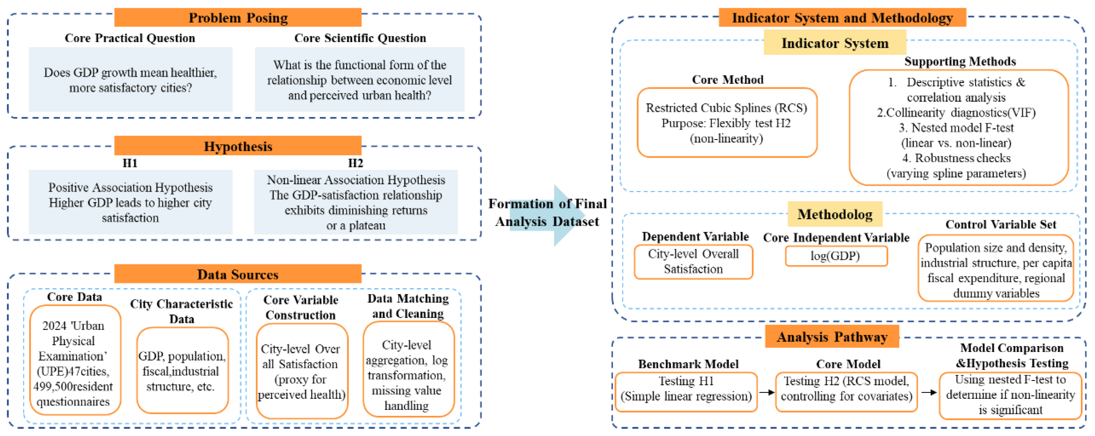
Figure 2.
GDP and spatial distribution map of sample cities.
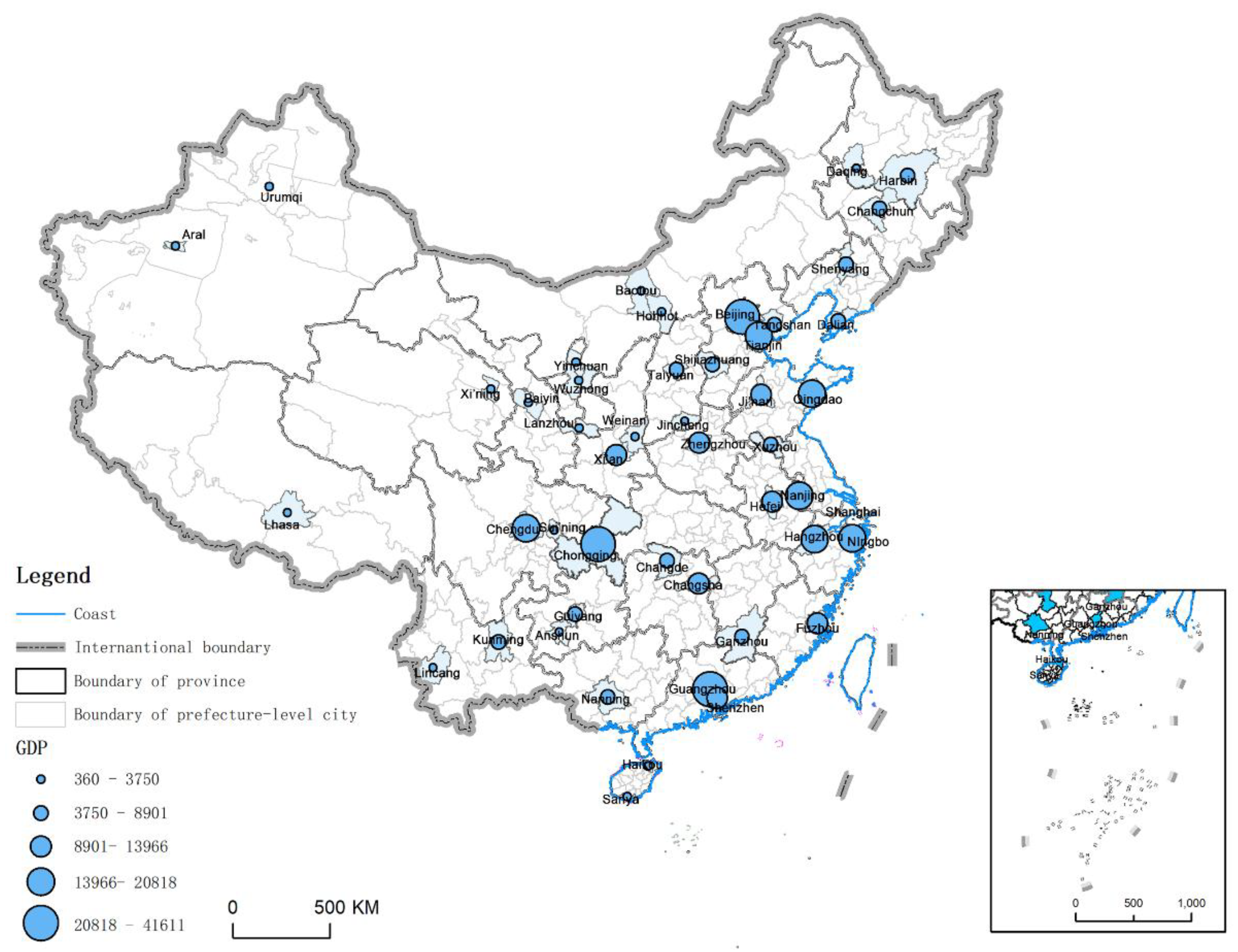
Figure 3.
Relationship between urban resident satisfaction and GDP chart and trend.

Figure 4.
Correlation matrix for the broader pool of city-level indicators.
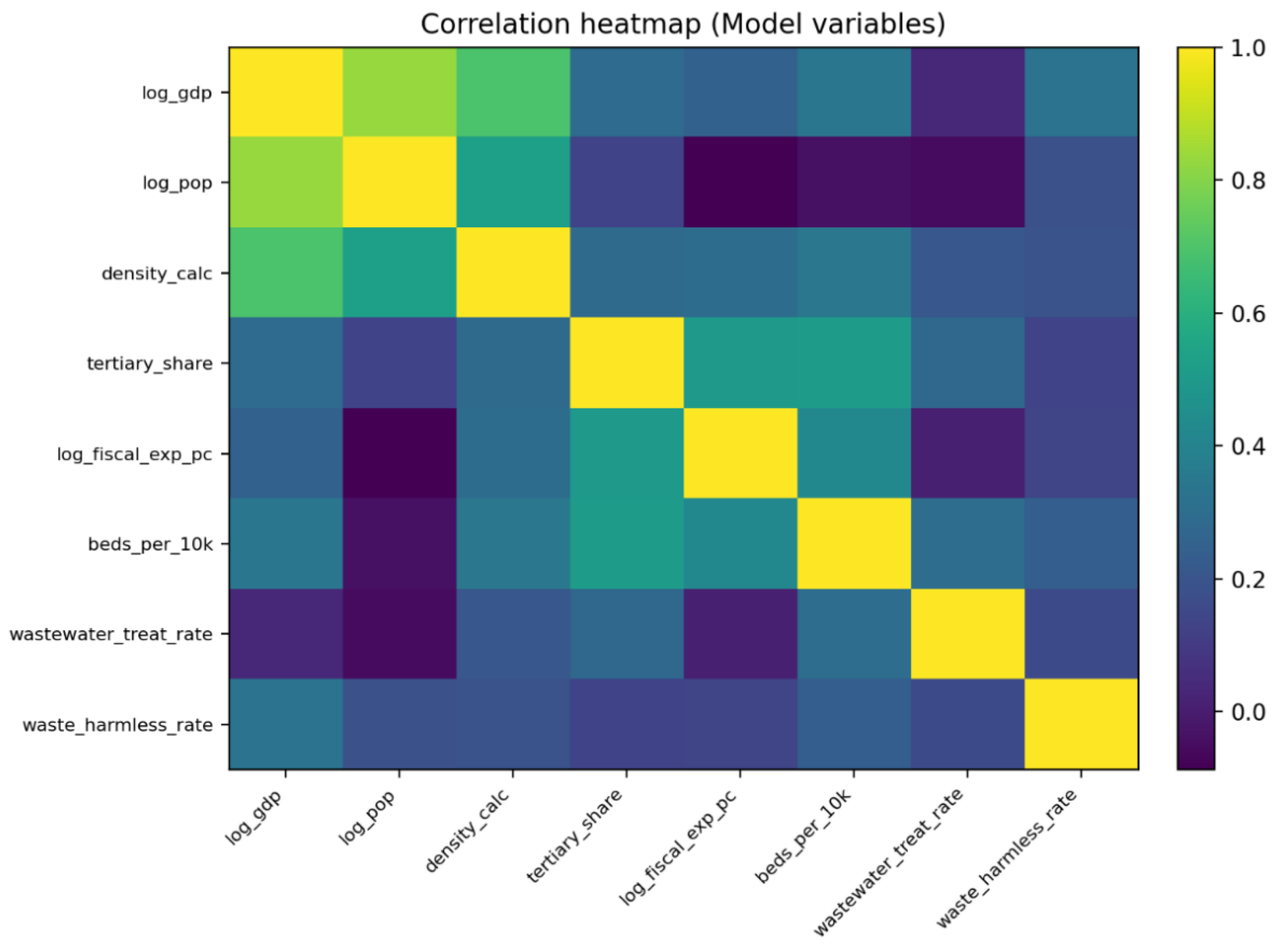
Figure 5.
The final indicators used in the econometric model.
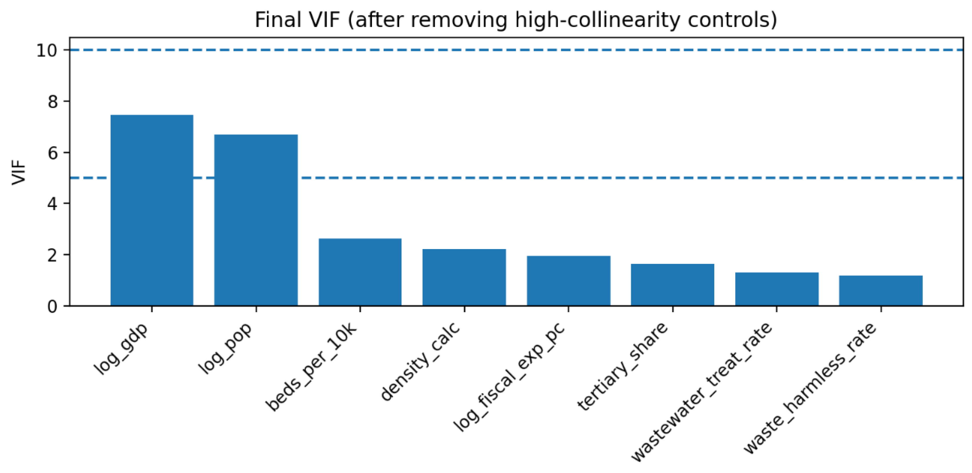
Figure 6.
Scatter plots of raw GDP vs. logGDP and overall city satisfaction.
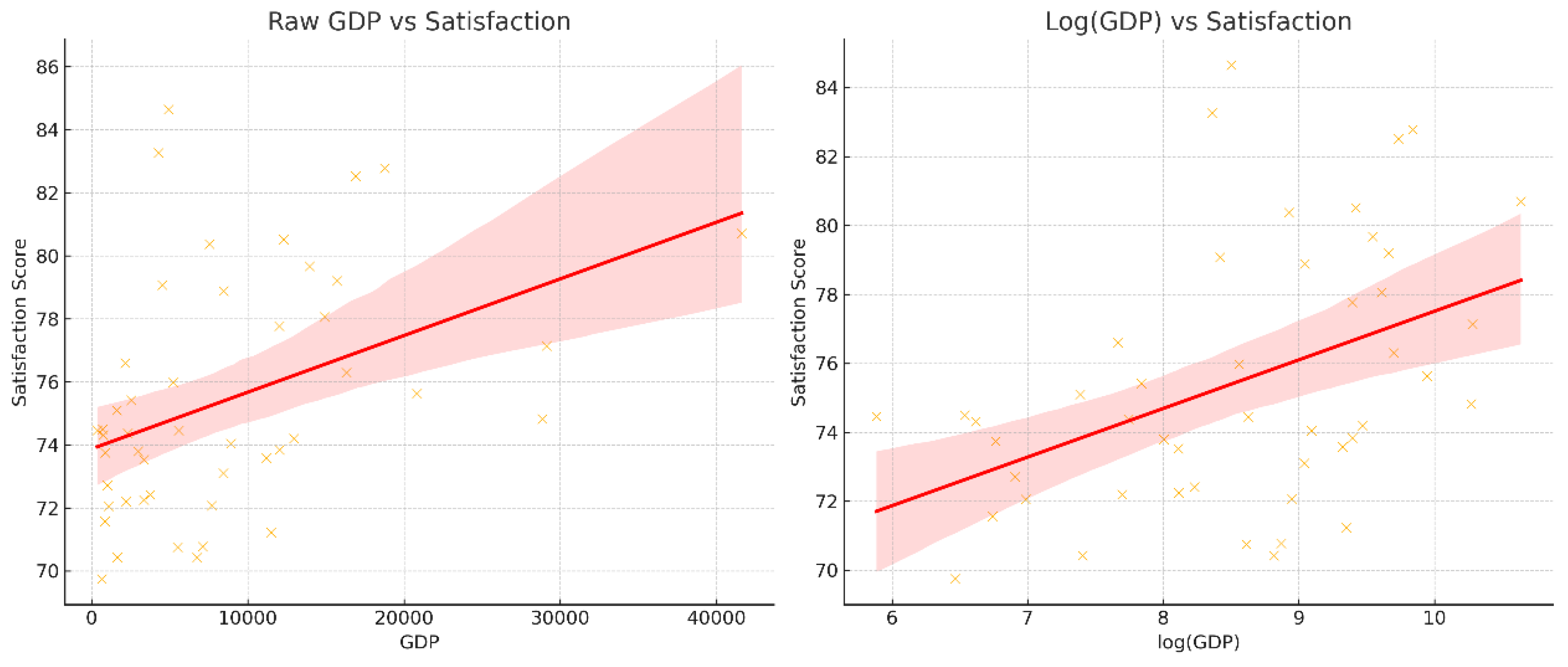
Figure 7.
RCS Models with Different Degrees of Freedom.
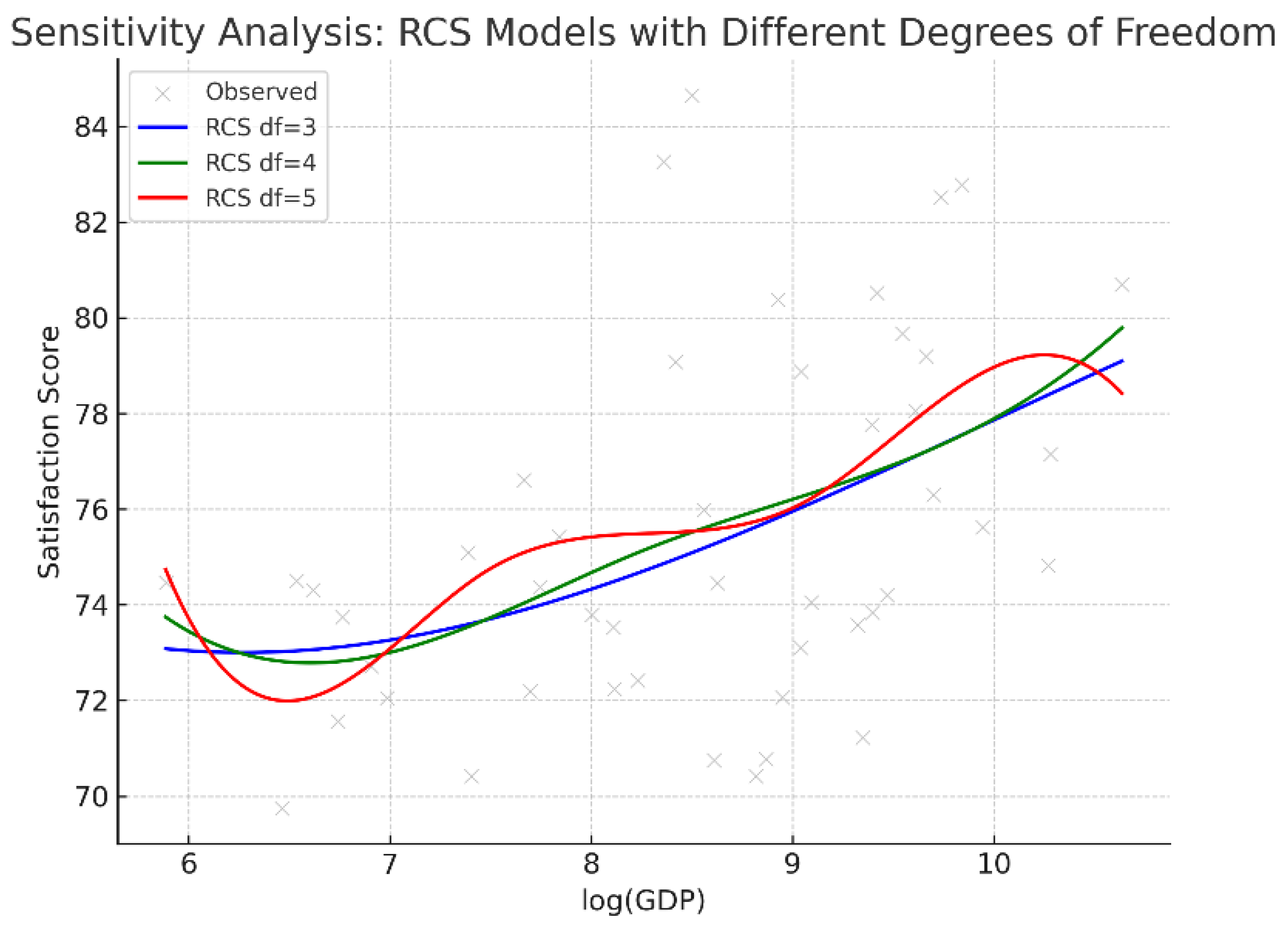
Figure 8.
RCS estimates of the GDP–satisfaction relationship (unadjusted).
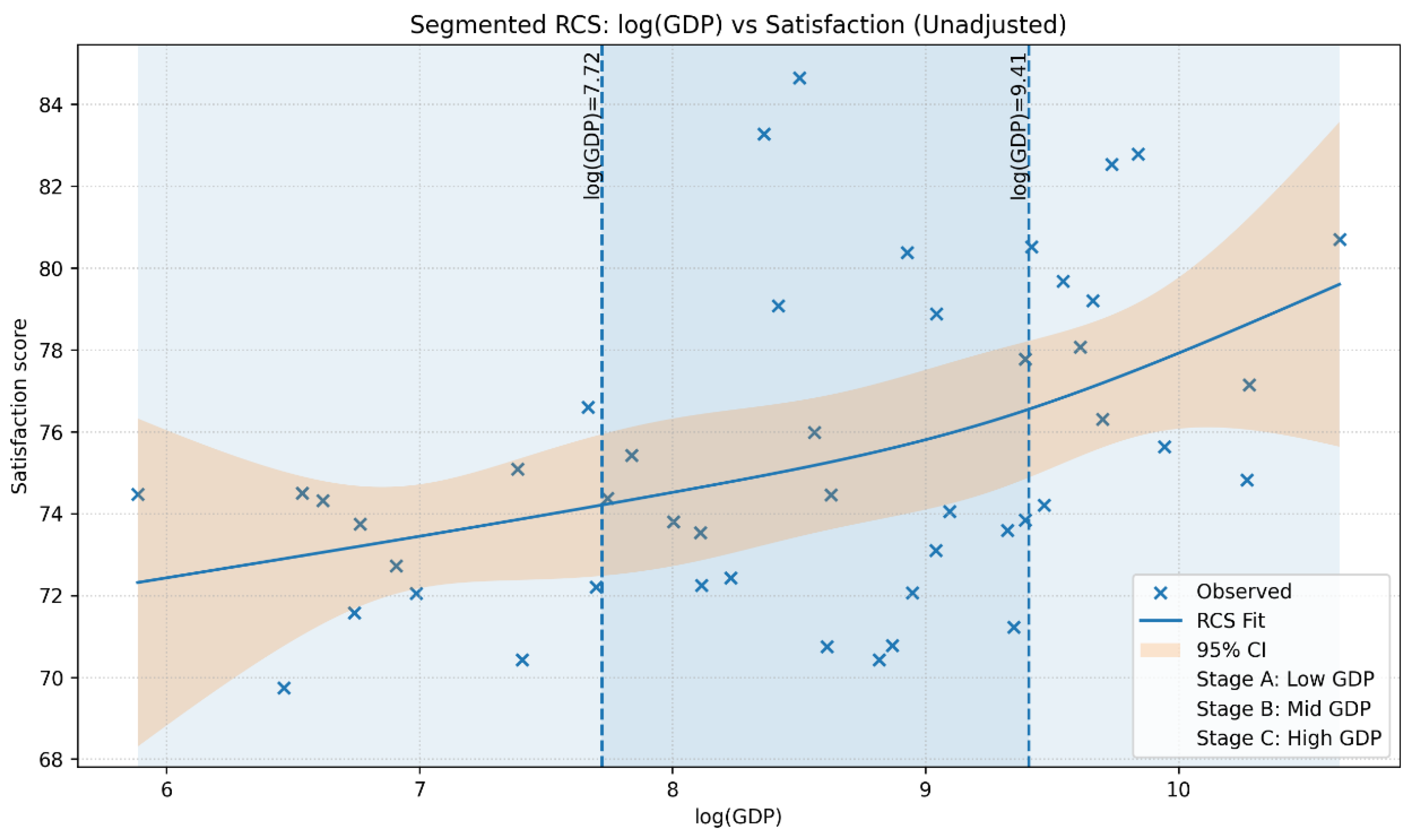
Figure 9.
RCS estimates of the GDP–satisfaction relationship (adjusted).
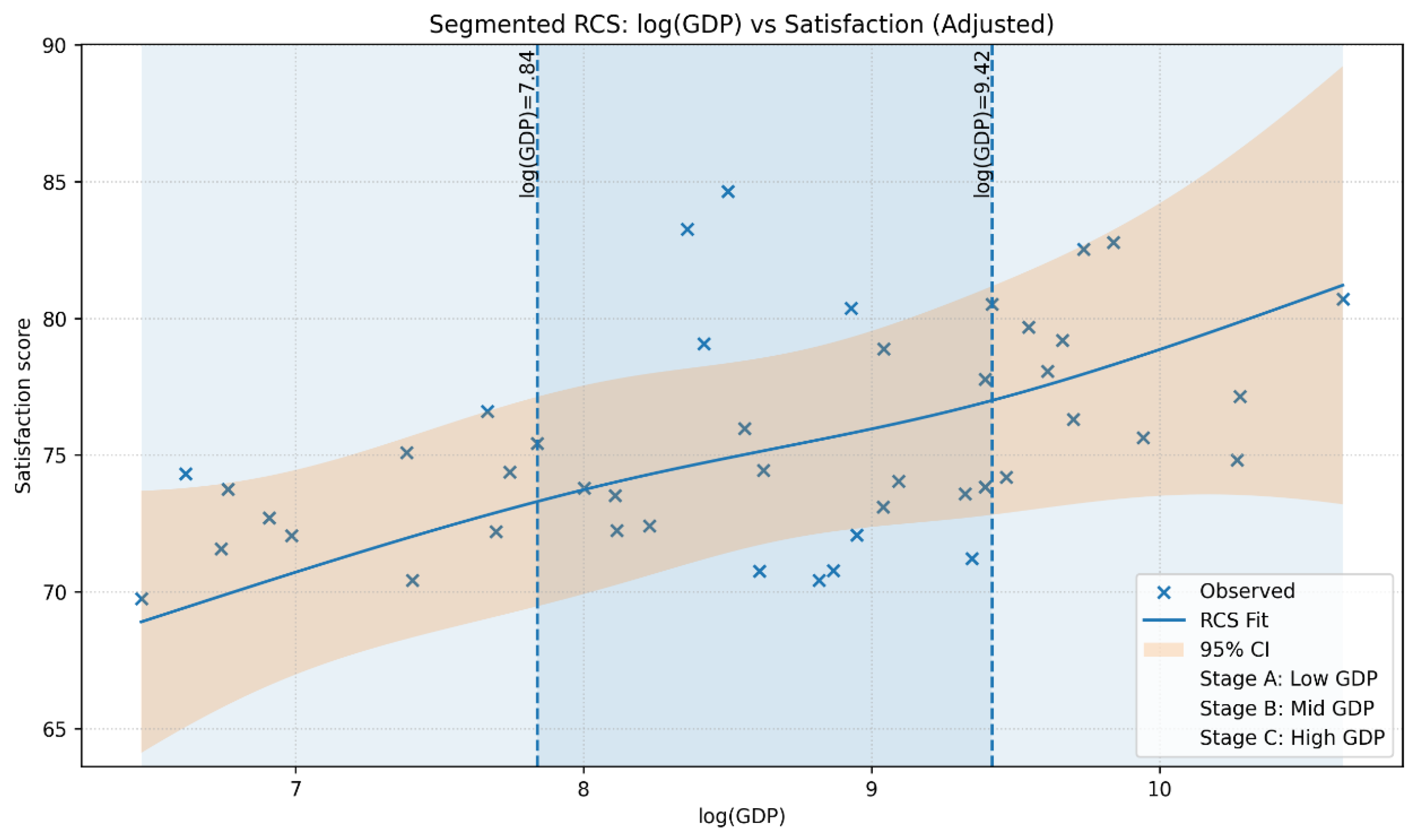
Table 1.
Descriptive statistics.
| Group | Variable | N | Mean±SD | Min–Max |
|---|---|---|---|---|
| Dependent variable | GDP (raw) | 47 | 8635.83±8641.56 | 360.00–41611.00 |
| log(GDP) | 47 | 8.52±1.17 | 5.89–10.64 | |
| Explanatory variables | Overall city satisfaction | 47 | 75.43±3.76 | 69.75–84.65 |
| Control variables | log(registered population) | 47 | 15.42±0.82 | 13.24–17.35 |
| Population density (persons/km²) | 47 | 520.47±324.64 | 18.97–1283.29 | |
| Tertiary industry share of GDP (%) | 47 | 57.58±10.17 | 38.82–83.52 | |
| log(fiscal expenditure per capita) | 47 | 9.62±0.61 | 7.06–11.09 | |
| Mechanism variables (optional) | Hospital beds (per 10,000 persons) | 47 | 68.97±22.10 | 32.17–128.21 |
| Wastewater treatment rate (%) | 47 | 96.14±3.45 | 84.19–107.29 | |
| Harmless domestic waste treatment rate (%) | 47 | 98.83±4.20 | 73.25–100.00 |
Note: Mean±SD denotes mean and standard deviation; Min–Max denotes minimum and maximum values; N is the number of valid observations.
Table 2.
Collinearity diagnostics.
| Variable | VIF | Tolerance |
|---|---|---|
| log(GDP) | 7.48 | 0.13 |
| log(registered population) | 6.7 | 0.15 |
| Hospital beds (per 10,000 persons) | 2.64 | 0.38 |
| Population density (persons/km²) | 2.23 | 0.45 |
| log(fiscal expenditure per capita) | 1.96 | 0.51 |
| Tertiary industry share of GDP (%) | 1.63 | 0.61 |
| Wastewater treatment rate (%) | 1.31 | 0.76 |
| Harmless domestic waste treatment rate (%) | 1.19 | 0.84 |
Note: VIF > 10 indicates severe collinearity; VIF > 5 warrants attention.
Table 3.
Comparison of RCS univariate model and full model parameters.
| Model | n | R2 | Adj_R2 | Nonlinearity_F | Nonlinearity_p |
|---|---|---|---|---|---|
| Model0_RCS_only | 47 | 0.1987 | 0.1427 | 0.2102 | 0.8112 |
| Model1_RCS+controls | 45 | 0.4063 | 0.2317 | 0.0848 | 0.9189 |
Disclaimer/Publisher’s Note: The statements, opinions and data contained in all publications are solely those of the individual author(s) and contributor(s) and not of MDPI and/or the editor(s). MDPI and/or the editor(s) disclaim responsibility for any injury to people or property resulting from any ideas, methods, instructions or products referred to in the content. |
© 2026 by the authors. Licensee MDPI, Basel, Switzerland. This article is an open access article distributed under the terms and conditions of the Creative Commons Attribution (CC BY) license (http://creativecommons.org/licenses/by/4.0/).
Copyright: This open access article is published under a Creative Commons CC BY 4.0 license, which permit the free download, distribution, and reuse, provided that the author and preprint are cited in any reuse.


