
Submitted:
13 January 2026
Posted:
14 January 2026
You are already at the latest version
Abstract
Small hydro power plants (HPPs) play an important role in managing fluctuating energy requirements. This article presents a real-world case study where model predictive control (MPC) utilizing lightGBM-based machine learning (ML) forecasts of energy demand and water availability is employed to optimize the scheduling of a small HPP for peak shaving. A comparative analysis is conducted between the current non-predictive control strategy, which relies on operator decisions for peak shaving, and a fully automatic controller that optimally schedules the utilization of available water resources based on ML predictions. Preliminary results show that the MPC can outperform the operator’s decisions and that this has the potential of improving peak shaving capabilities of small HPPs, emphasizing the role of predictive control methodologies for exploiting energy storage resource in the management of the distribution grid. This approach offers a pragmatic solution that small utilities can adopt with minimal effort using their own data.
Keywords:
model predictive control
; LightGBM
; energy demand forecast
; peak shaving
; hydro power plant
1. Introduction
Managing the variability of energy demand throughout the day poses a significant challenge for energy providers, potentially leading to increased electricity costs. As a result, utilities are increasingly concerned with effective storage and power generation strategies to address peak loads [1]. In the recent past, several techniques have been explored to reduce such undesired behaviour [2]. In particular, the optimal management of HPPs is considered effective for peak shaving purposes.
Most of the recent literature on the topic focuses on the optimal management of large installations. [3] proposes a composite model including multi-objective optimal peak shaving, inter grid power distribution and load fluctuation balance for the short term management of a massive system of 92 hydro power plants totalling 41GW nominal power. [4] formulated an improved daily peak shaving operation model for one-reservoir and multi-cascade hydropower stations by developing a method to represent water delay time and addressing non linear constraints for cascade hydropower stations. The main results demonstrate that the proposed Mixed-integer quadratic program (MIQP), integrating the delay time, effectively reduces peak-valley differences by 25% in the dry and 33% in the wet season. [5] proposed a decomposition and iterative search strategy (DISS) to address the challenges in short-term peak-shaving operation of complex, very large-scale hydropower installation with multiple reservoirs and cascades, which are characterized by modelling difficulties and high computational time. The DISS method involves dividing the system into independent subsystems, using mixed-integer linear programming (MILP) to find an initial feasible power output, and then iteratively refining the solution by adjusting peak-valley differences of the residual load. [6] addressed the challenge of coordinating the power dispatch of a cascade hydropower plants with pumping facilities to compensate for the increasing randomness of PV power. Authors propose a day-ahead dispatch strategy based on multi-objective stochastic optimization.
While most research focuses on large-scale hydropower installations, our work addresses the need for pragmatic, cost-effective solutions tailored to small utilities operating hydro power plants (HPPs) primarily for peak shaving. Small HPPs offer a dual advantage of environmental sustainability and operational flexibility, both essential for maintaining grid stability. These decentralized systems have the potential to contribute meaningfully to local peak load management, yet their capacity is constrained during dry periods due to the relatively low energy density of water storage. Effective management of this resource is therefore critical. In our region, we observed that such utilities often manage HPPs autonomously using non-optimized strategies, limiting their impact on grid flexibility. Similar situations have been observed in other areas [7]. Thanks to their many years of experience, operators ensure efficient utilization of resources and contribute to stable energy supply. However, their work, especially for less experienced personnel, can be supported by an optimal automatic scheduling system that suggests energy production plans aligned with the utility needs, including peak demand reduction and water preservation. Moreover, the decision-making and operational efficiency of operators can be enhanced by providing them with accurate forecasts of short-term energy demand and water availability.
To support operators in the scheduling task as well as the current trend toward semi or fully automated control in small HPPs, this study explores how automatic optimal scheduling of HPP production can meaningfully improve peak shaving efficiency. Achieving such improvement would also deliver economic benefits for utilities and end users, as power transfer prices paid by utilities increase linearly with peak demand. While this should incentivize peak reduction, adoption by small utilities is feasible only if solutions are agile, affordable, and easy to implement using existing historical data. Therefore, we propose an approach that leverages state-of-the-art ML models and MPC to smooth the load curve through optimal use of water storage during peak demand periods—without requiring complex or resource-intensive models.
1.1. Related Work
Approaches for optimal management of energy assets include Convex Optimization (CO) based control algorithms [8] and Multi-objective MILP for energy arbitrage in an energy community [9,10]. A simple Rule-Based Controller (RBC) is presented in [11] able to mitigate peak loads in the distribution grid of a Swiss utility. [12] and [13] propose more sophisticated approaches based on Genetic Algorithm and Binary Particle Swarm Optimization. Other techniques consider ML approaches such as [14] where authors propose a Decision Tree (DT) based approach for energy scheduling. Training the DT involves creating Learning Sets via Monte Carlo simulations, with short-term and long-term Firm Power Capacity provisions considered. Multi-agent Reinforcement Learning (RL) is considered in [15] where the RL controller employs Soft Actor-Critic agents to manage storage charging/discharging decisions. [16] compares MPC and RL, focusing on cost and carbon emissions. Results slightly favor MPC. Finally, [17] investigates RBCs and RL agents combining MaskPPO and a deep neural network.
We applied MPC in a previous study ([18]) to the flexible scheduling of residential energy loads for reducing the peak in the energy demand of a self-consumption community. The MPC based its decisions on estimations of the future energy demand from the flexibilities. This task was carried out by a predictive model combining a seasonal method with a simple classification model. This approach, which is used as a comparison baseline in this work, belongs to classical time-series forecasting methodologies (moving average, seasonal method with error correction, autoregressive models, etc.) that base their predictions on the most recent observations and assume specific patterns within a time series (trends and seasonal fluctuations)[19]. These approaches work well for short-term forecasting, while for medium to long-term forecasting it is important to include a set of explanatory variables or features, such as calendar effects, weather variations, and so on. Therefore, medium and long-term forecasting are more effectively treated as a regression problems [20].
In the last decade, several machine learning regression frameworks have been applied to time-series forecasts with covariates. Among them, lightGBM, a boosted tree-based algorithm, has proven very effective and popular, because, thanks to its versatility, effectiveness, and relatively simple usage, it allows obtaining models with competitive accuracy in relatively limited development times and computational resources [20,21,22]. For instance, boosted trees algorithms were one of the most used framework among those adopted by teams in the BigDEAL Challenge 2022, which was about energy load and peak forecasting [23]. They have also been successfully used in water availability forecasting [24]. Although studies on foundation models for energy forecasting are beginning to emerge and have shown promising results [25], they remain in an early stage, and their complexity and need for domain-specific adaptation place them beyond the scope of this work.
In this context, our research aims to develop an automatic MPC of the energy production of a small hydro power plant for load peak shaving and create forecasters of the energy demand and the water availability based on historical data from the utility. Such predictors serve a dual purpose: they inform the MPC’s decisions and provides valuable insights to the operator. Specifically, we focus on predicting energy demand and water availability over a two-day-ahead horizon with a 5-minute and 1-hour resolution, respectively. This requires to generate tens or hundreds of outputs (the target variable at each time steps of the two days ahead), making it a complex multi-output regression task. The forecasters are trained using LightGBM. However, lightGBM does not provide tools for multi-output regression. Traditional approaches to multi-output predictions are based on training multiple independent or chained models [26]. Some recent works, e.g. [27,28], have explored extensions of the gradient boosted trees framework to handle multiple outputs. We address the lack of native multivariate regression support by training a set of independent models for the water flow forecaster, while for the energy demand forecasts, due to the higher resolution of this time series, we designed a more efficient strategy that exploits LightGBM capability of handling missing data to learn a global model that is sufficiently accurate across the entire considered time horizon.
We demonstrate the proposed approach in the context of a small HPP managed by a local utility, the Azienda Elettrica di Massagno (AEM), and compare the operator decision to those of the MPC fed with different inputs. These experiments highlight the importance of feeding the MPC with accurate and reliable forecasts and show the potential of the MPC to support operators in their daily decision-making processes, thus enhancing energy storage management.
2. Materials and Methods
2.1. AEM Hydro Power Plant
We describe a real-word application of MPC for optimal management of water resources in the small-size HPP managed by AEM, a utility distributing energy primarily to the municipalities of Massagno, Capriasca and Isone in Ticino, Switzerland. The price of the electrical energy paid by AEM to the cantonal electricity supplier is based on both the energy volume and the power transfer price that is proportional to the peak demand reached each month. AEM exploits its HPP primarily to reduce peak demand, and thus contain the energy price.
The plant collects water from two rivers and accumulates it in a surge tank from which it can draw during peak demand periods, as described in Figure 1. The maximum production of the power plant is 4 megawatts, achieved at a water flow rate of 2.11 . The reservoir can store just over 17’000 of usable water, based on the specified minimum and maximum levels, corresponding to approximately 9 MWh of stored energy.
The production scheduling of the hydroelectric plant is a combination of real-time corrective control (that adjusts system operations in response to observed variations in demand) and operator decisions. The primary objective of the operators is to minimize the size of the monthly demand peak, which is usually observed during evenings. When the reservoir (surge tank) is full, the plant is set to reduce the monthly peak as much as possible. If the storage reservoir is not full, despite the goal of reducing peaks, the operators must also ensure that sufficient water volume in the reservoir will be available for the potential future consumption spikes. The operators determine the target value of the daily peak based on his/her expertise. They consider the current and short-term water availability, weather conditions and forecasts which influence both the demand and the future availability of water, the size of the peak already reached during the current month and the expected seasonal trends of the energy demand. A real-time corrective controller then schedules the production based on the difference between the most recently observed demand and the target peak value. Outside peak hours, production is limited by the need to fill the reservoir. If there is no need to fill the reservoir, the plant produces electricity based on the available water flow: the water entering the system is immediately utilized by the HPP to generate electricity. The operators can also intervene manually to directly schedule the production when weather conditions change.
2.2. Power Production Scheduling
The HPP we model within the MPC framework is a plant without pumping facilities, meaning that its reservoir is filled by inflow rivers only. This type of storage system has an uncontrollable inflow rate which can fill up the reservoir up to a maximum capacity (any excess water spills out when the storage is full).
The production of the HPP is managed using a MPC control strategy that models the system’s behaviour of interest over a finite time horizon, optimizes decisions for the immediate time step, and simulates future steps to anticipate the system’s trajectory. We define the duration and granularity of the horizon by an interval of time T, consisting of N steps, each of duration . In our experiments, T covers a 48-hours period starting from the current scheduling time , with granularity minutes, for a total of steps. The expected inflow rate at each future step , expressed in , as well as the energy demand are predicted at by the forecasters described in the next Section 2.3. The storage status is represented by the variable , expressed in , which denotes the estimated volume of water available at the end of step . Given these characteristics, the discharging power of the HPP at each timeslot is controlled via the continuous variable , as defined by the following set of equations.
where represents the amount by which the power requested from the grid exceeds the threshold , minimized over the 48-hours control horizon. The threshold represents the peak power recorded during previous days of the same month, since lowering the peak below that point would not improve the power transfer price. Constraints () ensure that captures the maximum amount by which the net value is expected to exceed at any time within T. Operational constraints () and () set the HPP to operate between given boundaries and without power changes larger than . Constraints () ensure that the HPP reservoir operates within a given interval. Finally, constraints () determine how the reservoir changes according to the selected power and the expected inflows of the rivers. Function is the discharge rate function that maps the power setpoint and the reservoir status to the amount of water consumed during a time slot of duration .
For the AEM HPP:
- All powers (, and ) are expressed in MW
- is set to MW
- P is set to 4MW
- is set to
- The water discharge in is obtained from the linear function , where 0.509 is the discharge rate at 1MW.
2.2.0.1. Post Optimization Settings
Based on HPP control experts, we implemented simple rule-based post-optimization decisions. When the estimated demand is “low” (i.e. below a parametrised threshold of the observed past peak) and the reservoir is “nearly full” (i.e. above a threshold, ) the HPP plant switches to self consumption mode preventing spillover while still generating some useful energy. In this mode, the plant adjusts its output to match the river inflow rate, while slowly filling the reservoir up to . The power output is computed using a convex combination:
where r weights between minimum power output and full inflow consumption. When the reservoir is just above the threshold, the plant minimizes output to allow filling; closer to full capacity, it matches self-consumption.
2.3. Energy Demand Forecasts
The goal of the energy demand predictive model is to forecast the utility’s energy demand over a 48-hours control horizon, with a resolution of 5 minutes. At the current time step , the model generates forecasts of the energy demand for each prediction time step , with . Model inputs include calendar features, past energy demand features and weather forecasts.
- Calendar features: they are both categorical (namely, day of the week, month, and a binary feature indicating holidays) and numerical (the sine and cosine of the day of the year and of the time of the day, to model circularity). These variables allow to capture the seasonal patterns.
- Past energy demand features: these include short-term lags (from 5 to 30 minutes behind with a step of 5 minutes) and medium-term lags of 1 day, 2 days, and 1 week. For medium-term lags, also the average, minimum, and maximum values over two time windows of 10 and 30 minutes are included.
- Weather forecasts: these include temperature, precipitations, and the average global horizontal irradiance (GHI), computed over 1 hour.
The features identified in this work are traditional in the context of energy forecasting [29]. We included a relatively large set of features covering a time horizon that is meaningful for this application. We did not apply explicit feature selection methods because LightGBM inherently performs feature selection during training. While different or more extensive feature sets could be explored, determining an optimal set was not the goal of this study, given the dataset’s specificity and the expectation that any improvement in predictive accuracy would be limited, being this a well explored domain, and, thus, not necessarily relevant for the control objective.
Given that LightGBM does not inherently support multi-output regression and since for this task we would need 576 outputs, we opted against constructing so many separate models. We adopted a strategy that learns only two single-output models. The first model is trained specifically for , as this forecast directly determines the only MPC decision that is actually implemented—subsequent decisions are revised as new information becomes available. The second model is used to provide forecasts for . Of the aforementioned predictor features , not all are available at for every value of h. For instance, short-term lags are not available for . The values of these unavailable inputs are left missing, exploiting the capability of the LightGBM algorithm to deal with missing values. As for the weather forecasts, the most recent forecasts available at time are used.
In the training phase, to account for all possible control horizons h, we adopt the following strategy. From each historical instance relative to some time t, we derive multiple training instances by considering different values of . For each of them, we set as missing all predictors that are not available at the sampled time . We also add h as an additional feature of the model. While in principle we could consider 576 different instances for each t, we choose to sample only 30 values of h, without replacement, for each historical instance, as keeping all of them would exceedingly increase the training dataset without adding much useful information to learn from. Sampling follows the non-uniform distribution , where is the number of hours corresponding to h, rounded up to the nearest integer. This approach weights more, during training, the shorter time horizons, for which more accurate predictions are both feasible and more valuable.
As a baseline for comparison with the LGBM-based demand forecaster, we adopt the statistical model introduced in [18], hereafter referred to as Stat. This model assumes daily periodicity in power demand and estimated values as the average demand observed at the same time of day over a sliding window including the past 10 days. For the first hour after , this 10-days average is combined with the demand at the current time by a weighted average assigning to a weight which decays with t as . To account for the weather conditions which may affect the demand, observations are classified into five categories, based on the observed temperature and irradiation conditions. For predicting the demand at a given future time t, only observations in the same weather category are averaged.
2.4. Inflow Forecasts
The goal of the inflow forecaster is to predict the reservoir inflow rate for the forecast horizons , , with hour. Since the output size is moderate, due to the lower resolution, we choose to use 48 different LightGBM models, each of which produces the forecast for h hours ahead. The forecaster is not directly trained to predict the future inflow rate, but the inflow rate variation . The models use as inputs date-time features, past inflow features and precipitation forecasts. Date-time features are the month and the sine and cosine of the day of the year and of the time of the day. Past inflow features include the last 6 observed values before time (i.e., for ) and the average, minimum, and maximum values of over a 6 and a 12 hours window before time . Precipitation forecasts include the predicted rainfall at the reservoir location, as well as the average rainfall forecasted at different positions along the rivers feeding into the reservoir. We use both the precipitation forecasts relative to 1, 2, and 3 hours before and the cumulative forecasted rain in the 2, 4, 6, 12, 18, 24 and 36 hours before .
3. Results
The analysis presented in this section are based on the data provided by the utility from December 2018 to August 2023. Due to technical problems with the utility data management system, data were lost for four long periods between December 2021 and March 2023, covering about 18 months. This affects the quality of the demand forecaster in that period. However, data from a total of 1184 days spread over 46 months are still available, which allow for training predictors that are good enough to demonstrate the merits of the proposed approach. We have selected four testing periods that are removed from the training data of the LGBM demand and flow rate forecasters: period 04/2021 (from 27.03 to 13.04.2021), period 08/2022 (from 1 to 28.08.2022), period 05/2023 (from 1 to 28.05.2023) and period 08/2023 (from 1 to 28.08.2023). The selection of test periods non-consecutive to training ones is thus motivated. We aimed to evaluate the model across diverse conditions, not only in different seasons but also in different years. This choice would be acceptable if similar energy demand patterns could be assumed before and after the testing period. In reality, however, demand patterns may evolve over time due to technological changes, such as increased PV penetration. Such changes could reduce model validity in the long term and may not necessarily improve forecast performance in the tested periods; in fact, they could even degrade it. In both cases, we expect the results to be slightly biased. The test on the last period (August 2023), taken at the end of the dataset, represents a good proxy for a realistic application scenario.
Over the four selected periods, we compare
- 1.
- the LGBM demand forecaster with the stat model from [18];
- 2.
- the LGBM water flow forecaster with the naive forecaster hereafter referred to as const, which assumes a flow rate constantly equal to the value observed at ;
- 3.
-
the MPC power production decisions in three input configurations with those historically executed by the HPP operator. The three configurations considered are:
- (a)
- the unrealistic oracle configuration, where the MPC knows the actual water flow rate or energy demand, which serves as upper bound for the MPC performance;
- (b)
- the LGBM configuration, when the MPC inputs are the demand and the water flow rate predicted by the LGBM models;
- (c)
- the stat configuration when the demand is predicted by the stat model and the flow rate by the naive cons forecaster.
The data provided by the utility include the historical energy demand time series (), the historical HPP power production (), the surge tank level and its inflow rate. The water availability at a given time t is obtained from a cubic relation with the the surge tank level derived from surge tank recovery measures provided by the utility. Weather forecast were purchased from the Swiss weather forecast provider MeteoBlue (https://content.meteoblue.com/en) and recorded by the utility only for the area supplied by the utility, while for the positions impacting the tank inflow, weather forecasts where taken from Open-meteo (https://open-meteo.com/). Unfortunately, Open-Meteo does not provide a history of past forecasts for years 2021-2023, but only the most recent forecast available for a given time. As a result, our evaluation may overestimate the performance of both the LGBM predictors and MPC, since we are partially relying on weather forecasts of higher quality than those that would have actually been available at any given time .
We observed inconsistencies between the measured inflow rate and the net inflow derived from the surge tank variation, , and the water consumed to produce , that is . Therefore, due to the higher reliability of power production and tank level records, in the following analyses, the measured inflow rate was replaced by its estimate :
The high variability of the resulting signal (see Figure 3) was attributed to measurement noise and was smoothed for training using a moving average with a 4-hours window.
Figure 2 (A) shows examples of the LGBM and (Stat) forecasts. We notice that LGBM systematically overestimates demand valleys during the 2023 period. This mismatch is mainly due to the increased penetration of photovoltaic (PV) installations, which has altered the demand patterns compared to previous years. The LGBM forecaster used for period 05/2023 and 08/2023 was trained assigning an increased weight to recent observations, but this was insufficient to solve the PV valleys issue, both because 2023 data is limited, as many entries were not properly recorded by the utility, and because total installed PV capacity is continuously increasing. In a similar situation currently under study, we found that providing the model with installed PV capacity as an input feature, when available, can improve its ability to capture PV-related patterns. However, since this issue affects only demand valleys and not the peaks, it is not critical in the context of this paper, and, to assess the model performance in the relevant peak hours, the metrics shown in Figure 2 (B) and (C) to compare the two models across different forecast horizons, are computed considering only the time steps in which the demand exceeds the median demand for that day. Such comparison highlight that, by accounting for the predicted weather conditions, LGBM achieves better accuracy starting already from a 20-minute ahead forecast. LGBM outperforms Stat also in the 5-minutes ahead forecast, since a model specifically trained for this prediction horizon is used in this case. A similar analysis is conducted for the water flow forecaster in Figure 3. The predicted signal appears significantly smoother than the observed data, and that the LGBM flow rate forecaster consistently outperforms the constant flow baseline, except in very short-term forecasts, where their performance is comparable.
Figure 4 and Table 1 analyse the MPC performance across the four simulation periods. For each day, the maximum net energy demand (daily peak) was calculated. Figure 4 compares the distribution of daily peaks, contrasting the operator’s performance with the MPC’s under the three input configurations considered. For each period, we computed the mean and the maximum values of the daily peaks and performed a paired t-test for the mean difference in the peak values achieved by the MPC and the operator. Since each analyzed period corresponds to a specific month, the maximum daily peak value directly determines the power transfer price and, consequently, the cost of the energy purchased by the utility. To further quantify the MPC ability to flatten the load curve, we computed the load fluctuation index as in eq.(8).
where is the net demand at time t, is the number of time steps in period and the average net demand over . The Load Fluctuation Index (LFI) provides a measure of how much the net energy demand deviates from its average value over a given period: the higher the LFI, the more pronounced the peaks and valleys, whereas a lower LFI indicates a flatter and more stable demand profile. This metric is computed as the average relative deviation of each time step from the period’s mean demand, as shown in Equation (8).
4. Discussion
From the boxplot and from the average and maximum peak values, we observe that the MPC peaks are smaller, on average, than those achieved by the operator and its ability to flatten the load curve, as measured by the LFI, is larger across all periods and in all input configurations, except occasionally in the Stat configuration which generally performs worse than the others. The p-values in Table 1 show that the mean MPC difference with the operator peaks is almost always significant (p-value<0.01). However, the maximum peak of the period can sometimes be higher for the MPC. This is evident, for example, in period 04/2021 for both LGBM and stats, and in period 08/2023 for all configurations. These higher peaks typically occur due to water shortages during peak times, caused by overestimated inflow, or underestimated demand. This highlights how the operator’s more conservative approach can sometimes be preferable. However, in the extremely dry period of 08/2022, such a conservative approach resulted in the operator decision to keep the facility at minimal output, thus giving up on mitigating the peaks. In contrast, the automatic MPC concentrated water use, though limited, during peak hours, significantly reducing them. Figure 5 shows an example of MPC simulation results from this period. The first two plots display the actual demand and water flow, along with the LGBM forecasts made at for the next 48 hours. The third plot compares the operator’s and MPC’s decisions, the fourth shows the resulting net energy demand requested from the grid, and the fifth illustrates the water volume available in the surge tank. It can be noticed that the MPC exploits the available water mostly during peaks, thus managing to flatten them much more than the operator doeas, since, in the scarcity of water, he operated a more conservative strategy. Even in this period, by blindly relying on forecasts, the deterministic MPC occasionally faced water shortages during peaks, leading to the two outliers in the LGBM boxplot of Figure 4. While there is still room for improvement, the MPC strategy proves overall more effective than the operator’s conservative one, and could be improved, in future work, by implementing stochastic optimization strategies that, by accounting for forecast uncertainty, would achieve more robust decisions.
According to the tariffs and remuneration rates for the transmission grid published by swissgrid.ch, which outlines the tariff structure applied to power consumption and grid services in Switzerland, we can assume a power tariff of 50 kCHF per MW. A power tariff refers to the cost charged for the maximum power capacity (or peak load) contracted or used, rather than the energy consumed over time. Based on this assumption and the difference in peak load between the operator and the scheduler, ranging from -1 MW to +2 MW, with an average of 0.3 MW over the 4 simulated periods, we can estimate an average monthly saving of approximately 16 kCHF. This amount should be considered in light of the relatively small size of the plant.
5. Conclusions
This article explores the application of Model Predictive Control to optimize the production scheduling of small hydroelectric power plants. The primary objective is to leverage the plant’s flexibility to reduce peak electricity demand from the grid, thereby lowering energy costs. The findings demonstrate that automated scheduling can enhance operator decision-making, offering a support that is particularly valuable during periods of water scarcity, when effective scheduling is most critical.
This work originated from a need observed across multiple local utilities, and likely shared by similar operators worldwide. We adopted a well-established approach to build predictive models using the relatively small datasets typically available to individual utilities, without aiming for state-of-the-art forecasting performance, the goal being to demonstrate the feasibility and effectiveness of such methods in combination with MPC in this real-world context, rather than outperforming advanced modeling techniques. Results show clear advantages over the current reactive control and operator-based decisions; however, compared to an oracle scenario with perfect knowledge of demand and inflow, forecast inaccuracies can significantly increase daily and monthly peaks and the controller may exhibit over sensitivity to prediction errors. Therefore, improving prediction models and controller robustness remains two important direction for future work.
Forecast accuracy, e.g, by expanding the training dataset through aggregation of records from similar utilities and hydroelectric reservoirs; by adapting the model to reflect emerging energy demand patterns associated to the increased photovoltaic power installed; and by exploiting when possible recent advanced on foundational model for energy forecasts [25]. Additionally, upgrading the MPC to incorporate probabilistic forecasts would enable more robust decision-making by better managing the prediction uncertainty.
Building on these findings, future research should focus on improving forecast accuracy, e.g., by expanding training datasets through aggregation of records from similar utilities and hydroelectric reservoirs and leveraging recent advances in foundational models for energy forecasting [25]; devise model updating framework able to adapt models to reflect emerging demand patterns driven by technological and social changes, such as increased photovoltaic penetration; upgrading the MPC to incorporate probabilistic forecasts would enable more robust decision-making by explicitly accounting for prediction uncertainty.
Data Availability Statement
Data and code supporting the findings of this study are available from the corresponding author upon request and subject to prior authorization from the utility.
Acknowledgments
This project has received funding in the framework of the joint programming initiative ERA-Net Smart Energy Systems’ focus initiative Digital Transformation for the Energy Transition, with support from the European Union’s Horizon 2020 research and innovation programme under grant agreement No 883973.
References
- Abdelfattah, A.I.; Shaaban, M.F.; Osman, A.H.; Ali, A. Optimal Management of Seasonal Pumped Hydro Storage System for Peak Shaving. Sustainability 2023, 15, 11973. [Google Scholar] [CrossRef]
- Chua, K.H.; Bong, H.L.; Lim, Y.S.; Wong, J.; Wang, L. The state-of-the-arts of peak shaving technologies: a review. In Proceedings of the 2020 International Conference on Smart Grid and Clean Energy Technologies (ICSGCE), 2020; IEEE; pp. 162–166. [Google Scholar]
- Wu, X.Y.; Cheng, C.T.; Shen, J.J.; Luo, B.; Liao, S.L.; Li, G. A multi-objective short term hydropower scheduling model for peak shaving. International Journal of Electrical Power & Energy Systems 2015, 68, 278–293. [Google Scholar] [CrossRef]
- Liao, S.; Liu, Z.; Liu, B.; Cheng, C.; Wu, X.; Zhao, Z. Daily peak shaving operation of cascade hydropower stations with sensitive hydraulic connections considering water delay time. Renewable Energy 2021, 169, 970–981. [Google Scholar] [CrossRef]
- Zhao, H.; Liao, S.; Fang, Z.; Liu, B.; Ma, X.; Lu, J. Short-term peak-shaving operation of “N-reservoirs and multicascade” large-scale hydropower systems based on a decomposition-iteration strategy. Energy 2024, 288, 129834. [Google Scholar] [CrossRef]
- Wang, Z.; Li, Y.; Wu, F.; Wu, J.; Shi, L.; Lin, K. Multi-objective day-ahead scheduling of cascade hydropower-photovoltaic complementary system with pumping installation. Energy 2024, 290, 130258. [Google Scholar] [CrossRef]
- Grigoras, G.; Gârbea, R.; Neagu, B.C. Toward Smart SCADA Systems in the Hydropower Plants through Integrating Data Mining-Based Knowledge Discovery Modules. Applied Sciences 2024, 14, 8228. [Google Scholar] [CrossRef]
- Babacan, O.; Ratnam, E.L.; Disfani, V.R.; Kleissl, J. Distributed energy storage system scheduling considering tariff structure, energy arbitrage and solar PV penetration. Applied Energy 2017, 205, 1384–1393. [Google Scholar] [CrossRef]
- Terlouw, T.; AlSkaif, T.; Bauer, C.; van Sark, W. Multi-objective optimization of energy arbitrage in community energy storage systems using different battery technologies. Applied Energy 2019, 239, 356–372. [Google Scholar] [CrossRef]
- Kriett, P.O.; Salani, M. Optimal control of a residential microgrid. Energy 2012, 42, 321–330. [Google Scholar] [CrossRef]
- Efkarpidis, N.A.; Imoscopi, S.; Geidl, M.; Cini, A.; Lukovic, S.; Alippi, C.; Herbst, I. Peak shaving in distribution networks using stationary energy storage systems: A Swiss case study. Sustainable Energy, Grids and Networks 2023, 34, 101018. [Google Scholar] [CrossRef]
- Zhang, S.; Tang, Y. Optimal schedule of grid-connected residential PV generation systems with battery storages under time-of-use and step tariffs. Journal of Energy Storage 2019, 23, 175–182. [Google Scholar] [CrossRef]
- Hannan, M.A.; Abdolrasol, M.G.M.; Faisal, M.; Ker, P.J.; Begum, R.A.; Hussain, A. Binary Particle Swarm Optimization for Scheduling MG Integrated Virtual Power Plant Toward Energy Saving. IEEE Access 2019, 7, 107937–107951. [Google Scholar] [CrossRef]
- Moutis, P.; Hatziargyriou, N.D. Decision trees aided scheduling for firm power capacity provision by virtual power plants. International Journal of Electrical Power and Energy Systems 2014, 63, 730–739. [Google Scholar] [CrossRef]
- Nweye, K.; Sankaranarayanan, S.; Nagy, Z. MERLIN: Multi-agent offline and transfer learning for occupant-centric operation of grid-interactive communities. Applied Energy 2023, 346, 121323. [Google Scholar] [CrossRef]
- Zhan, Sicheng.; Lei, Yue.; Chong, Adrian. Comparing model predictive control and reinforcement learning for the optimal operation of building-PV-battery systems. E3S Web of Conf. 2023, 396, 04018. [Google Scholar] [CrossRef]
- Rocchetta, R.; Nespoli, L.; Medici, V.; Basso, S.; Derboni, M.; Salani, M. Rule-based deep reinforcement learning for optimal control of electrical batteries in an energy community. In Proceedings of the Proceedings of the 33rd European Safety and Reliability Conference (ESREL 2023), 2023; pp. 639–646. [Google Scholar]
- Author(s), A. Hidden for review.
- Bontempi, G.; Ben Taieb, S.; Le Borgne, Y.A. Machine learning strategies for time series forecasting. Business Intelligence: Second European Summer School, eBISS 2012 Tutorial Lectures 2 2013, Brussels, Belgium, July 15-21, 2012; pp. 62–77. [Google Scholar]
- Rubattu, N.; Maroni, G.; Corani, G. Electricity Load and Peak Forecasting: Feature Engineering, Probabilistic LightGBM and Temporal Hierarchies. In Proceedings of the International Workshop on Advanced Analytics and Learning on Temporal Data, 2023; Springer; pp. 276–292. [Google Scholar]
- Ke, G.; Meng, Q.; Finley, T.; Wang, T.; Chen, W.; Ma, W.; Ye, Q.; Liu, T.Y. LightGBM: A Highly Efficient Gradient Boosting Decision Tree. In Proceedings of the Advances in Neural Information Processing Systems; Guyon, I., Luxburg, U.V., Bengio, S., Wallach, H., Fergus, R., Vishwanathan, S., Garnett, R., Eds.; Curran Associates, Inc., 2017; Vol. 30. [Google Scholar]
- Zhang, Y.; Ma, R.; Liu, J.; Liu, X.; Petrosian, O.; Krinkin, K. Comparison and explanation of forecasting algorithms for energy time series. Mathematics 2021, 9, 2794. [Google Scholar] [CrossRef]
- Shukla, S.; Hong, T. BigDEAL Challenge 2022: Forecasting peak timing of electricity demand. In IET Smart Grid; 2024. [Google Scholar]
- Akbarian, M.; Saghafian, B.; Golian, S. Monthly streamflow forecasting by machine learning methods using dynamic weather prediction model outputs over Iran. Journal of Hydrology 2023, 620, 129480. [Google Scholar] [CrossRef]
- Ferdaus, M.M.; Dam, T.; Sarkar, M.R.; Uddin, M.; Anavatti, S.G. Foundation models for clean energy forecasting: A comprehensive review. Renewable and Sustainable Energy Reviews 2026, 226, 116452. [Google Scholar] [CrossRef]
- Mastelini, S.M.; da Costa, V.G.T.; Santana, E.J.; Nakano, F.K.; Guido, R.C.; Cerri, R.; Barbon, S. Multi-output tree chaining: An interpretative modelling and lightweight multi-target approach. Journal of Signal Processing Systems 2019, 91, 191–215. [Google Scholar] [CrossRef]
- Nespoli, L.; Medici, V. Multivariate boosted trees and applications to forecasting and control. Journal of Machine Learning Research 2022, 23, 1–47. [Google Scholar]
- Zhang, Z.; Jung, C. GBDT-MO: gradient-boosted decision trees for multiple outputs. IEEE transactions on neural networks and learning systems 2020, 32, 3156–3167. [Google Scholar] [CrossRef]
- Wen, Q.; Liu, Y. Feature engineering and selection for prosumer electricity consumption and production forecasting: A comprehensive framework. Applied Energy 2025, 381, 125176. [Google Scholar] [CrossRef]
Figure 1.
Scheme of the AEM hydro power plant.
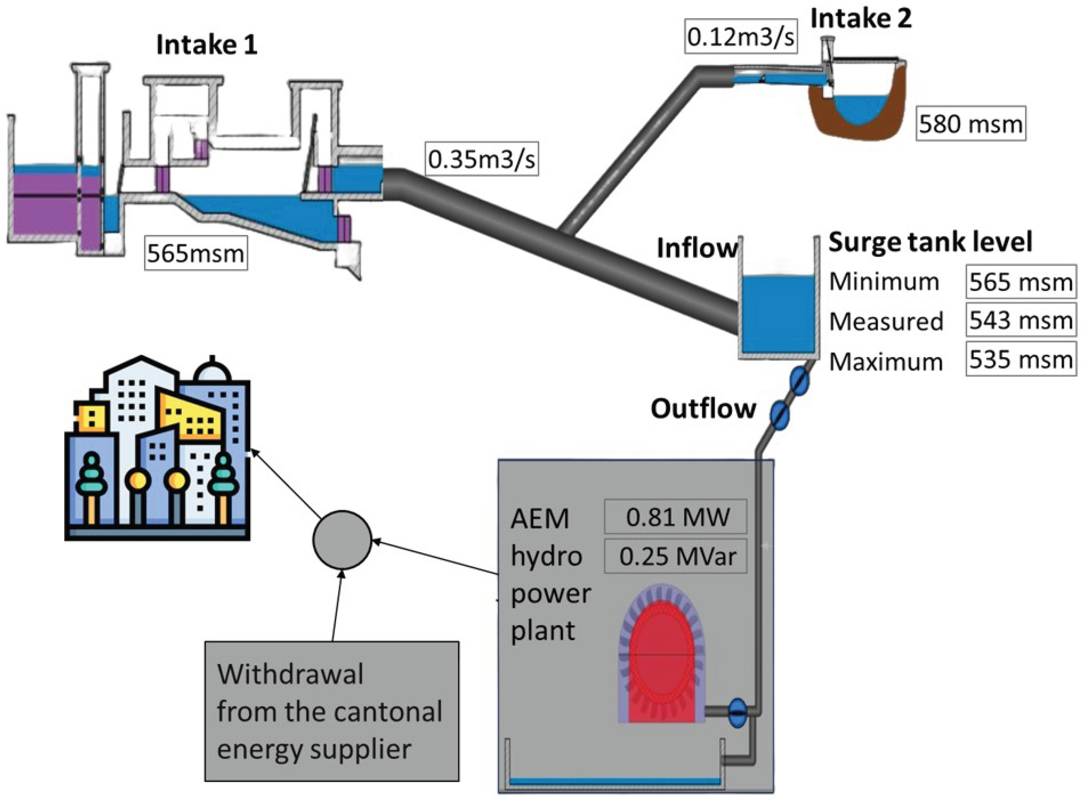
Figure 2.
(A) Example of energy demand forecasts. (B) root mean square error (RMSE) and (C) symmetric mean absolute percentage error (sMAPE) of the LGBM and stat predictors.
Figure 2.
(A) Example of energy demand forecasts. (B) root mean square error (RMSE) and (C) symmetric mean absolute percentage error (sMAPE) of the LGBM and stat predictors.
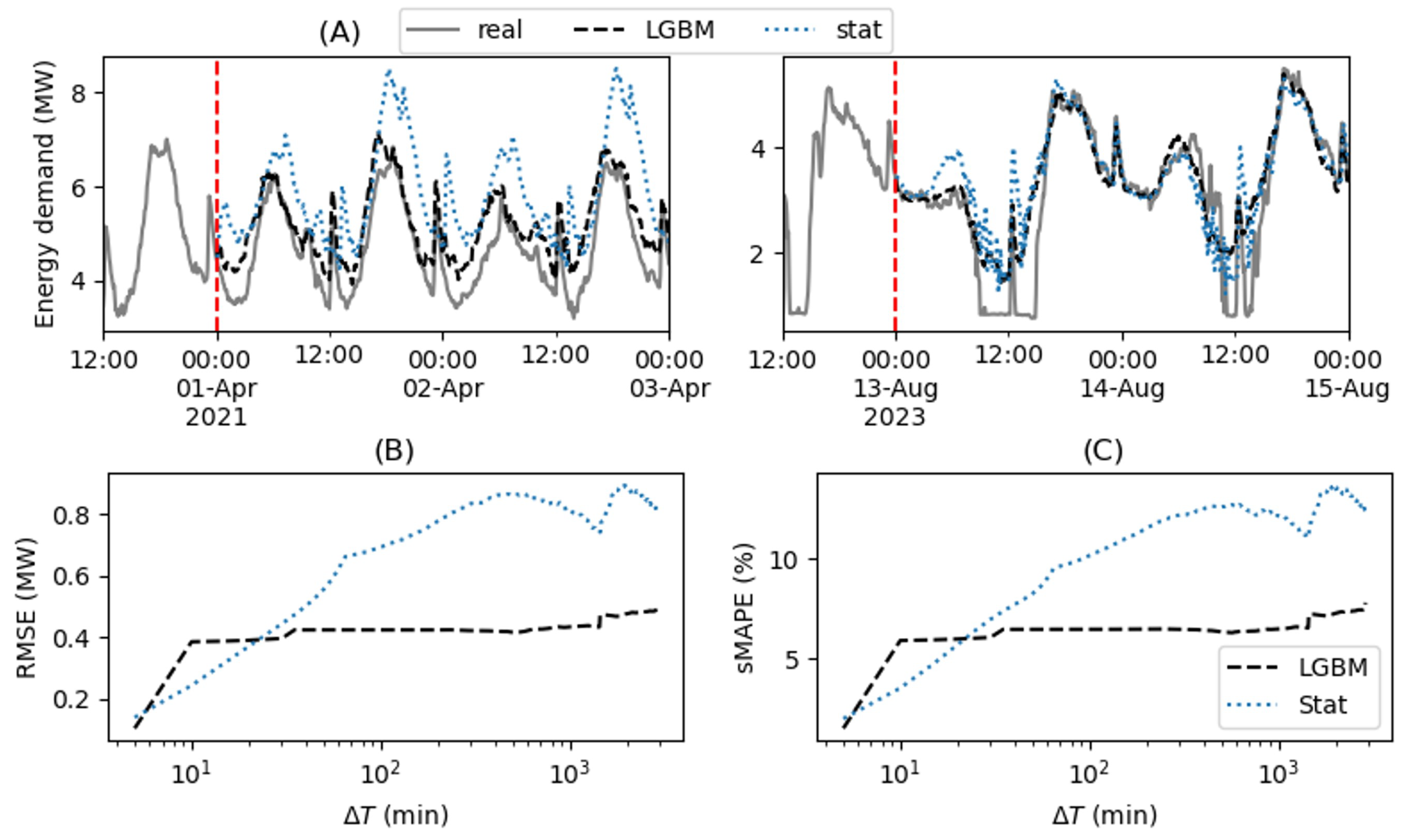
Figure 3.
(A) Example of water flow forecasts. (B) RMSE (C) sMAPE of the LGBM and constant flow predictors.
Figure 3.
(A) Example of water flow forecasts. (B) RMSE (C) sMAPE of the LGBM and constant flow predictors.
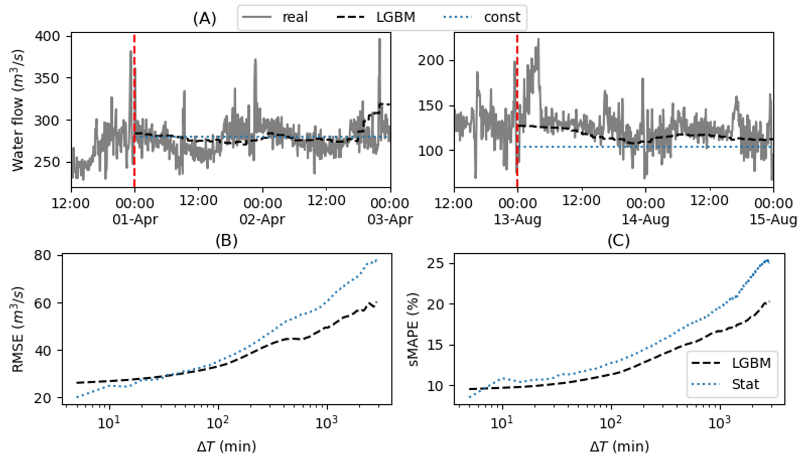
Figure 4.
Boxplots of the daily peaks distribution in the different periods and under different settings.
Figure 4.
Boxplots of the daily peaks distribution in the different periods and under different settings.

Figure 5.
Dashboard with the MPC output.
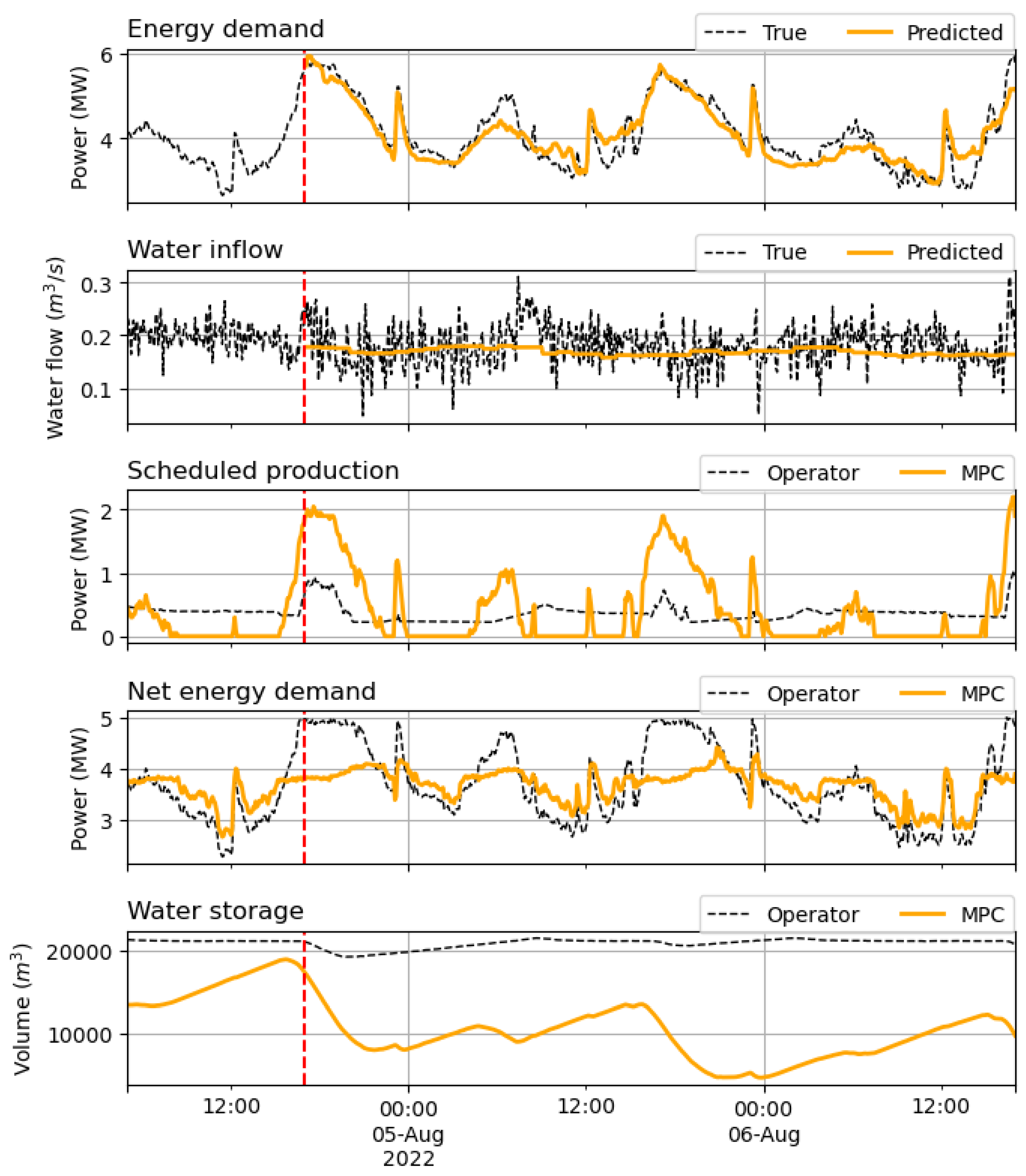

Table 1.
Peak shaving performance achieved by the operator or the MPC in the oracle and LGBM and stat configurations. LFI stands for Load Fluctuation Index; mean and max refer to the average and maximum values of daily peaks, respectively; p-val indicates the significance of the mean difference in peak values achieved by the operator and the MPC.
| LFI | max | mean | p-val | LFI | max | mean | p-val | |
|---|---|---|---|---|---|---|---|---|
| 04/2021 | 08/2022 | |||||||
| operator | 0.257 | 6.53 | 5.30 | - | 0.207 | 6.50 | 5.03 | - |
| oracle | 0.203 | 6.00 | 4.79 | 4e-3 | 0.100 | 4.61 | 4.02 | 5e-9 |
| LGBM | 0.202 | 7.45 | 5.04 | 0.11 | 0.103 | 5.76 | 4.11 | 7e-14 |
| Stat | 0.222 | 7.41 | 5.70 | 0.898 | 0.121 | 5.26 | 4.45 | 1e-6 |
| 05/2023 | 08/2023 | |||||||
| operator | 0.564 | 5.55 | 3.77 | - | 0.407 | 4.47 | 3.61 | - |
| oracle | 0.351 | 3.32 | 2.72 | 9e-10 | 0.267 | 4.51 | 3.22 | 3e-6 |
| LGBM | 0.394 | 3.55 | 2.83 | 2e-12 | 0.300 | 5.00 | 3.38 | 0.010 |
| Stat | 0.415 | 4.85 | 3.07 | 1e-7 | 0.315 | 5.21 | 3.71 | 0.863 |
Disclaimer/Publisher’s Note: The statements, opinions and data contained in all publications are solely those of the individual author(s) and contributor(s) and not of MDPI and/or the editor(s). MDPI and/or the editor(s) disclaim responsibility for any injury to people or property resulting from any ideas, methods, instructions or products referred to in the content. |
© 2026 by the authors. Licensee MDPI, Basel, Switzerland. This article is an open access article distributed under the terms and conditions of the Creative Commons Attribution (CC BY) license.
Copyright: This open access article is published under a Creative Commons CC BY 4.0 license, which permit the free download, distribution, and reuse, provided that the author and preprint are cited in any reuse.


