
Submitted:
12 January 2026
Posted:
13 January 2026
You are already at the latest version
Abstract
A composite, eighteen-year long record on in-situ surface meteorology and computed bulk air-sea fluxes of heat, freshwater, and momentum from an ocean site windward of Oahu are presented. Data were logged every minute over eighteen years. Methods and data quality are discussed. Statistics of one-minute, one-hour, and one-day times series are presented, and daily averaged time series provide an overview of this trade wind site. Mean wind was 6.8 m s−1 toward the west southwest, mean ocean heat gain was 23.2 W m−2 with freshwater loss of 1.2 m yr−1. Energetic sub-diurnal variability was found, with spectral peaks in solar insolation and sea level pressure, and transient, short-lived signals including insolation above the clear sky value, short periods of warm air, and downdrafts of dry air. Mean daily cycles are presented. Longer lasting events, including periods of ocean cooling, ocean heating, and hurricanes, are explored. Mean annual cycles are presented. The ocean loses heat from January through early May; then gains heat until late October and returns to loosing heat. Normalized by duration, the events examined have potential for significant contributions to the heat, freshwater, and mechanical energy exchanges.
Keywords:
air-sea flux
; surface meteorology
; trade wind
; long record
; rapid sampling
; heating and cooling events
; daily and annual cycles
1. Introduction
The oceanic trade wind regions cover close to 50% of the ocean surface. The trade winds originate in the mid-latitude high pressure regions and flow westward towards the equator where there is ascension in the intertropical convergence zones. During their passage across the ocean there is opportunity for exchanges of heat, freshwater, and momentum between the atmosphere and ocean. There has long been interest in better understanding this coupling between the ocean and atmosphere in the trade wind regions and the role these regions play in weather and climate.
On shorter time scales, the daily cycle of solar insolation and the modulation of incoming radiation by clouds in the trade wind regions has been of interest. The collaborative ASTEX (Atlantic Stratocumulus Transition Experiment) in 1992, for example, sought to better understand cloud dynamics and marine boundary layer processes in the eastern tropical Atlantic [1]. The VOCALS-ReX field study [2] investigated cloud dynamics, boundary layer processes, and the modulation of surface radiation by stratocumulus clouds in the trade wind region of eastern South Pacific in 2008.
Interest in air-sea coupling in the trade wind regions extends from the processes at work on daily to weather time scales to variability at interannual and decadal time scales. Studies have looked at links between the trade wind regions and climate variability and at the realism of models in representing surface meteorology and air-sea exchanges in the trade wind regions. Li et al. [3] used winds from atmospheric reanalyses over 1900 to 2010 to identify strengthening trade winds in the western equatorial Pacific and weakening trade winds in the eastern equatorial Pacific and investigate links between these trends and Pacific climate modes. Yang et al. [4] used monthly winds from the ERA5 reanalysis to look at Pacific trade wind variability between 1950 and 2020 and found strengthening winds in the 1990s with accompanying lowering of sea level pressure and sea surface temperature (SST). Simpson et al. [5] found when comparing global climate model surface wind stress in the trade wind regions to that from reanalyses which do assimilate observations that the climate models yield stronger than observed zonal-mean surface winds. Weller et al., [6] compared surface meteorology and air-sea fluxes from three reanalyses to close to 20-year long, withheld, observed surface meteorology and air-sea flux time series at three trade wind sites and found that reanalyses mean stress magnitudes were higher than observed and also that reanalysis multi-year mean net air-sea heat fluxes were between 5 and 30 W m−2 lower than observed.
Motivated by the desire to better understand the surface meteorology and air-sea exchanges of heat, freshwater, and momentum, long-term deployments of well-instrumented surface moorings have been carried out at the three trade wind sites, two in the Pacific and one in the Atlantic [6]. The intent was to build long, climate quality, withheld time series and to document the accuracies and statistics and characteristics of those time series. Because the observations are withheld, the time series provide references for comparison to models, remote sensing, and hybrid products, and the sites have been called Ocean Reference Stations. In this paper we begin to report on analysis of the time series from the Ocean Reference Station (ORS) at the Pacific site north of Oahu. Our plan is to write a series of papers to first document the observed surface meteorology and air-sea flux time series at periods up to and including one year; second, document the observed interannual variability; third, investigate the role of sub-annual processes and events in contributing to the observed interannual variability; and finally, present a more detailed comparison between the observations and atmospheric models across all time scales than that presented earlier in Weller et al. [6].
The site providing the observations presented here is an oceanic site north of Oahu, Hawaii. The record has a basic sampling rate of once per minute and spans over 20 years. Time series of surface meteorology and computed air-sea fluxes with one-minute, one-hour, and one-day sample rates are produced from the observations. This paper describes and examines the variability at periods ranging from one minute to one year. The deployments began in 2004. The duration and high temporal resolution contribute to the uniqueness of the time series. Some long records of surface meteorology from land sites exist and have been presented and discussed (e.g., [7,8]; and [9]). In the past, time series of ocean surface meteorology were collected from ships at the Ocean Weather Stations [10]. Fissel et al. [11], for example, reported on 10 years of Ocean Weather Station P data. Since the end of the Ocean Weather Ship occupations, observations and reporting of surface meteorology and collection of long oceanic time series with collocated surface meteorology and air-sea fluxes have required sequential deployments of surface moorings. The U.S. National Data Buoy Center (NDBC), for example, maintains surface buoys that provide surface meteorological and surface wave observations that are telemetered and assimilated into operational models [12]. The Upper Ocean Processes Group (UOPG) at the Woods Hole Oceanographic Institution (WHOI) and other research groups have developed well-instrumented surface moorings to observe air-sea fluxes of heat, freshwater, and momentum as well as surface meteorology and worked to maintain select observing sites. The time series discussed here is from one such site of sustained surface mooring deployments. This site north of Oahu is easy to reach for maintenance cruises sailing out of Pearl Harbor; yet, being positioned 120 km north of the island in a region of prevailing northeast trade winds, it is not in the island’s leeward wake [13] and provides information about the broader local trade wind region.
This is the first in the series of papers focused on the surface meteorological and air-sea flux of heat, freshwater, and momentum time series from the site north of Oahu. Reported here is the analysis of data from deployments 1 to 17 (August 13, 2004 to July 25, 2022) spanning 18 years with a focus on characterizing the observed variability across the span of one-minute to one-year periods. Section 2 discusses the observational methods and assessments of the quality of the observations. Section 3 overviews the 18-year records using daily-averaged time series of surface meteorology and air-sea fluxes; record-long plots and histograms based on the full record are presented. To explore variability not captured in daily averages, Section 4 starts with a table comparing statistics of the one-minute and one-hour time series with those for one-day time series. Large differences between different averaging periods in several variable’s maxima and minima motivate further discussion of sub-diurnal period variability in Section 4. First, frequency spectra of one-minute time series are discussed and then energetic but transient signals, including those responsible for one-minute minima and maxima, are examined using one-minute sampled time series. Section 5 uses the record long one-hour time series to characterize the mean daily cycle of the surface meteorological and air-sea flux variables. As in all sections after the discussion of the methods, the cumulative heat, freshwater, and mechanical energy transfer between the atmosphere and ocean are reported. Section 6 moves on to examine variability at periods of days to months with the goal of characterizing the meteorological variability and air-sea exchanges during different regimes. Five events are described, ocean heating under low winds, ocean heat loss in fall, a second period of ocean heat loss in winter, a period of summer heating including Hurricane Darby, and Hurricane Douglas. To document strong seasonal cycles in many variables, the mean annual cycles are presented in Section 7. Section 8 provides a summary and compares the cumulative heat, freshwater, and mechanical energy transfers for the events described in the paper and summarizes findings.
2. Observational Methods and Air-Sea Flux Computation
The Upper Ocean Processes Group (UOPG) at WHOI (Woods Hole Oceanographic Institution) has worked to maintain sustained observations from three ORS [6] including the site north of Oahu. The goals in maintaining the sites are to recover complete, ongoing, accurate time series of surface meteorology to support multidisciplinary studies, to contribute to the collection of oceanic surface meteorology and air-sea fluxes as part of the international OceanSITES element of the Global Ocean Observing System, and to provide an independent basis for assessing model-based and remote sensing derived ocean surface variables. To obtain the ongoing record, annual deployments of a fresh surface mooring are made, overlapping the previously deployed mooring. To maximize the likelihood of collecting a complete set of meteorological observations, redundant sensors are deployed. Work has been done to quantify the uncertainties in these surface meteorological observations and in the derived bulk formula air-sea fluxes (e.g., [14]), and the high-quality time series are available (http://uop.whoi.edu). The telemetered surface meteorology is withheld from the Global Telecommunications System (GTS) and thus from assimilation by operational models. These observations can thus serve as benchmarks or references for assessing models. We have previously noted [6] that comparisons between WHOTS observations and air-sea fluxes and those from the NCEP2 [15], ERA5 [16], and MERRA2 [17] show significant differences in long-term means and low-pass filtered time series.
2.1. The WHOTS ORS Site and the Surface Mooring
The data collection started in August 2004 using a well-instrumented surface mooring maintained at a site 120 km north of Oahu, Hawaii through cooperation between the WHOI UOP group and colleagues at the University of Hawaii at Manoa. The observations come from the sequential deployments of the WHOTS (Woods Hole Oceanographic Institution Hawaii Ocean Timeseries Station) surface mooring at Station Aloha, north of Oahu. The site is that of the long running Station ALOHA (~4700 m water depth) where ongoing oceanographic studies began in 1988 (http://aloha.manoa.hawaii.edu). The surface mooring also supports ongoing atmospheric CO2 time series observations by NOAA PMEL [18], which complement the atmospheric CO2 observations made on Mona Loa since the 1950s (https://gml.noaa.gov/obop/mlo/).
The WHOTS ORS is maintained in coordination with the ongoing Hawaii Ocean Timeseries (HOT) program. Two sites 12-14 km apart, within the ALOHA site (Figure 1) are used on an alternating basis. A fresh mooring is deployed before the prior mooring is recovered to facilitate QC (Quality Control) and quantify consistency. Cruises to the site to recover and deploy the moorings are planned annually, and all but one has been conducted as planned. The WHOTS 16 mooring was in the water for 692 days when
There was no cruise in 2020. Appendix 1 provides a table listing the deployment and recovery times and anchor location for each deployment.
2.2. The Quality of ORS Surface Meteorological Observations
Recovery of the deployed mooring is generally preceded by deployment of a new surface mooring with freshly calibrated sensors at the alternate site. On most of the mooring turn-around cruises, high quality meteorological sensors have been deployed on the ship to cross-compare buoy and ship-based measurements. These additional shipboard meteorological sensors were deployed by colleagues from the NOAA Physical Sciences Laboratory, Boulder, CO (e.g., [21]). The UOP group also routinely mounted freshly calibrated, stand-alone ASIMET modules on the vessel. For the cross-comparison between the two buoys and the ship, one to several days of meteorological data are collected with the ship near the moorings and oriented into the wind if possible. At the new buoy, comparisons with shipboard sensors provide an immediate check on the meteorological measurements. If agreement between ship and buoy meteorological sensors is poor, ASIMET modules on the buoy are replaced. At the old buoy, the shipboard observations provide an in-situ end of deployment assessment of the sensors against the chance that they are damaged on recovery and not available for post-calibration. After the in-situ intercomparison the old mooring is recovered. Recovered ASIMET modules are photographed, and data spikes induced (for example, by putting covers on the shortwave radiometers and placing SST sensors in ice water) to check the instruments’ clocks and allow for refining the time bases. Once recovered, meteorological instruments are shipped back to WHOI for post-calibration.

Table 1.
Sensors used at WHOTS in the ASIMET systems with typical heights. Actual heights are measured and recorded for each deployment. Specific humidity (SH) is computed using the observations.
Table 1.
Sensors used at WHOTS in the ASIMET systems with typical heights. Actual heights are measured and recorded for each deployment. Specific humidity (SH) is computed using the observations.
| Observable | Sensor make and model | Typical height above sea surface | Notes |
|---|---|---|---|
| Wind (WSPD) | RM Young 5103 | 3.3 m | Propeller-vane anemometer, stock propeller bearing upgraded |
| Wind (WDIR) | Gill Instruments WindObserver II Ultrasonic Anemometer | 3.3 m | Sonic anemometer, used at times to mitigate data loss due to birds |
| Air temperature/humidity (Ta/RH) |
Rotronic MP-101A | 2.95 m | Porous Teflon filter and multiplate radiation shield |
| Incoming shortwave radiation (DSWR) | Eppley Precision Spectral Pyranometer | 3.43 m | Case adapted to ASIMET module tubing |
| Incoming longwave radiation (DLWR) | Eppley Precision Infrared Radiometer | 3.43 m | Case adapted to ASIMET module tubing |
| Barometric pressure (SLP) | Heise DXD | 3.0 m | With parallel plate pressure port |
| Precipitation (P) | RM Young 50202 | 3.12 m | Self-siphoning rain gauge |
| Sea surface temperature and salinity (SST, SSS) |
SeaBird 37 MicroCAT |
-.75 to -.85 m | Mounted on buoy bridle |
One-minute time series are quality-controlled for each deployment, and successive deployments are added to a merged, long record. In the merging process, differences between simultaneous observations from the two buoys are resolved by comparing the overlapping records to the shipboard observations. When new information is available about calibration or processing procedures, the deployment-by-deployment data are reprocessed and updated merged time-series created.
There are no gaps in the surface mooring occupancy of the WHOTS ORS. Sensor issues were restricted to the wind and to rainfall. Wind direction was lost during Hurricane Darby in July 2016 and was lacking until the next deployment in 2017. A short period later wind speed observations stopped due to damage by sea birds. For the 2016-2017 deployment the missing hourly wind speed data were filled using ERA5 wind speed based on fitting overlapping WHOTS and ERA5 winds. The fit for wind speed was ERA5 WSPD = 0.97 x WHOTS WSPD -0.5 m s−1; WHOTS hourly east winds were filled using ERA5 WNDE = 1.064 x WHOTS WNDE + 0.3392 m s−1; and WHOTS north winds were filled with ERA5 WNDN = 0.9782 x WHOTS WNDN–0.2003 m s−1. The short gap later was filled in the same way. The other sensor issue was with the rain gauges. The rain gauges are self-siphoning cylinders which, at times, can be clogged by guano. The two ASIMET rain gauges are compared and for recent deployments a third, piezoelectric rain sensor has been deployed to aid in QC. Overall, with these wind sensor issues and excepting rainfall, a 99.5% complete one-minute record runs from 2004 to the present.
There was one additional post-recovery processing step taken in this analysis. Buoy-ship and buoy-buoy comparisons, confirmed with laboratory calibrations, found that the amplifiers used in the first generation DLWR ASIMET modules had small shifts in the gain and offset of the amplifier when the module was powered off and then on again. These early DLWR modules were used in the first three deployments; later deployments used DLWR modules with new, stable amplifiers. The DWLR recorded in the first three deployments was corrected to bring its mean to the mean of the fourth deployment, and the amplitude of the swing between clear sky and cloudy sky DLWR values was scaled to match that of the fourth deployment.
Over the years work has been done to assess the accuracy of the ASIMET sensors in the field. Colbo and Weller [14] analyzed the differences between the redundant, coincident one-minute samples recorded on ORS buoys and found differences occur from sensor aging, environmental impacts, and clock drift in the time bases of different sensors. They used probability distributions of the difference time series to obtain 50% and 95% confidence limits for each sensor type, as well as the standard deviation of each of the uncorrected one-minute time series, to quantify measurement accuracy in the one-minute time series. With averaging over several minutes, the accuracies improve greatly. Table 2 summarizes the uncertainty assessments for the WHOTS surface meteorological records that have been stated and used to gauge comparisons with models [6]. To provide a context for the uncertainty estimates, Table 2 also shows the record-long means. Further work on ASIMET sensor accuracies in the field can be found in Bigorre et al. [22], Weller [23], and Weller et al. [6]. Recently, Schlundt et al. [24] did a detailed intercomparison of wind observations from four UOP group surface moorings with scatterometer winds. They found a root-mean-square difference of 0.56 to 0.76 m s−1 between buoy and scatterometer winds. Part of the work included modelling flow distortion errors on the buoys. In processing ORS wind record, small differences in wind direction (~2-5°) had been noted from the redundant anemometers on the buoy (Figure 2). The modelling of flow distortion around the buoy hull and tower by Schlundt et al. [24] showed, depending on the angle of the wind relative to the buoy, the anemometers were affected by the distortion, with error up to 5% of the wind speed in the most affected sensor. The results from Schlundt et al. [24] allow the identification of the anemometer with the least error, but we have not yet incorporated doing so in the QC processing. In their analysis of the ORS in the North Atlantic Bigorre and Plueddemann [25] added consideration of the flow distortion errors (4%) and buoy tilt error (4%) to estimate WSPD error of 8% or 0.4 m s−1. Other sensor errors in Bigorre and Plueddemann [25] were close to those in Table 2.
2.3. Air-Sea Flux Computation and Quality Assessment
The quality-controlled surface meteorological time series are used together with the COARE 3.0 bulk formulae (Fairall et al. [26,27]) to compute heat, freshwater, andmomentum fluxes. Colbo and Weller’s [14] error propagation equations for the
Table 2.
Summary of the WHOTS accuracies for one-minute observations, daily averages, and annual means (after Colbo and Weller [14] and Weller [23]). For context, the mean values for the merged WHOTS 1 to 17 record are shown. Except for wind velocity and rain rate, all are means of January 1, 2005 to December 31, 2021. For those, calendar years that included gaps were omitted. Wind direction is based on the record mean WNDE and WNDN.
| Sensor | WHOTS mean | One-minute | Daily | Annual |
|---|---|---|---|---|
| Downward longwave (W m−2) (DLWR) |
388.8 | 7.5 | 4 | 4 |
| Downward shortwave (W m−2) (DSWR) |
238.1 | 20 | 6 | 5 |
| Relative Humidity (%RH) (RH) |
75.6 | 1 3 (low winds) |
1 3 |
1 |
| Air temperature (°C) (Ta) |
24.26 | 0.2 (more in low wind) | 0.1 | 0.1 |
| Barometric pressure (hPa) (SLP) |
1017.0 | 0.3 | 0.2 | 0.2 |
| SST (°C) | 25.15 | 0.1 | 0.1 | 0.004 |
| Wind speed (m s−1) (WSPD) |
6.77 | 1.5% or 0.1 (more in low wind) |
1%, 0.1 (max of these) |
1%, 0.1 (max of these) |
| Wind direction (°) (WDIR) |
264.0 | 6 (more in low wind) | 5 | 5 |
| Rainfall (% under catchment) (Prate, mm hr−1) |
.06 | 10% | 10% | 10% |
COARE 3.0 bulk formulae (Fairall et al., [26,27]) are used estimate the uncertainties in the computed fluxes. Abbreviations used for the flux terms are net air sea heat flux (QN), net longwave radiation (Ql), net shortwave radiation (Qs), latent heat flux (QH), sensible heat flux (QB), rain heat flux (QR), wind stress magnitude (τ), east wind stress component (τE), north wind stress component (τN), and wind stress direction (τdir). QR is computed under the assumption that rainwater hitting the sea surface is at the dew point temperature. Table 3 summarizes the accuracies of the bulk formulae fluxes used in Weller et al., [6]. Further discussion including consideration of the use of the COARE algorithm is available in Bigorre at al. [22] and Weller et al. [6]. When Bigorre and Plueddemann [25] included the additional error in wind speed, their error estimates of daily QB, QH, and QN were 2.5, 12, and 15.5 W m−2, respectively.
3. An Overview of Surface Meteorology and Air-Sea Fluxes at WHOTS
3.1. Surface Meteorology Time Series—An Overview Using Daily-Averages
Daily averaged time series spanning WHOTS 1 to 17 provide an overview of the surface meteorological record (Figure 3). Annual cycles are evident in SST, Ta, SH, and incoming shortwave. The annual cycle in DLWR is smaller in amplitude (~10 W m−2) with minima lagging those in DSWR by about 3 months. In the winter, the variability of Ta, SLP, SH, Prate, DSWR, and WSPD is higher, but mean values of SLP, DSWR, and SH are lowest. Sea surface temperature is warmer than air temperature in the mean, and upward spikes are evident. In contrast, the air temperature time series has downward spikes. The vector wind time series (Figure 3) shows that the variability in WDIR is greater during the winter and departures from southwesterly flow are associated with synoptic weather events.
The wind rose (Figure 4) shows the dominance of the ENE trade winds in the region where the WHOTS ORS is located. Figure 4 also shows the histograms of the daily averages of the surface meteorology. While humidity (SH), SLP, and DLWR are the most normally distributed though with negative skewness, SST and DSWR are bimodal. The bimodal SST distribution stems from its annual sinusoidal variability; one peak centered near the long-term mean late winter SST minimum of 23.8 °C and the other near the long-term mean late summer maximum SST of 26.8 °C. Although Ta generally tracked SST, its histogram lacks as pronounced a peak for winter conditions as seen in SST; and the time series plots shows cool Ta events during the winters. The absence of a winter peak is due to the negative skew associated with variable cold air advection during winter.
For DSWR there is also an annual cycle, but the distribution is not symmetric around the mean value. The WHOTS ORS being just inside the Tropics (±23.46°), the sun passes overhead twice each year, once in late May and again in mid-July. Winter clouds can only reduce the DWSR relative to summer, fair weather trade wind conditions, so there is a negative skew to that distribution of daily averaged values. The peaks in the histogram of DSWR are close to the long-term mean winter and the summer values of 158 W m−2 and 305 W m−2.
The population of daily rain rates is dominated by low rain rate events, < 4 mm hr−1, though several high rain rate events, up to 13 mm hr−1 extend the histogram. Rain is episodic, and the logarithmic scaling of the time series plot of rain rate (Figure 3) was done to capture the range of rain rate events. The daily rain rate maximum was associated with hurricane Darby in July 2016. SLP is negatively skewed by cyclonic systems (winter storms, Kona lows, and tropical cyclones) occasionally passing near WHOTS.
3.2. Air-Sea Flux Time Series—An Overview Using Daily Averages
Daily averaged time series provide an overview of the air-sea flux record (Figure 5). Gaps in the hourly wind time series were filled with adjusted hourly ERA5 winds as described earlier to compute the flux time series. Strong annual cycles are evident in QN and QS. Ocean heating (QN > 0) was seen spring to fall, with ocean cooling in the winter. Smaller annual cycles are seen in QH and Ql. Air-sea fluxes in winter-spring and fall show greater variability and larger amplitude signals. Cloud cover events in winter led to downward spikes in QS. Together with events of strong QH they contributed to strong, short-lived ocean cooling events seen in daily QN but not as evident in 10-day smoothed QN. The record-long accumulation of rain reached close to 10 m, while record long evaporation was close to 30 m.
Figure 6 shows histograms of daily averaged heat fluxes and wind stress. QN and QH are strongly skewed negative with asymmetric distributions due to small numbers of strong ocean heat loss events. The asymmetry in QB also reflects the occurrence of a small population of the strongest sensible heat loss events. Wind stress magnitude is strongly skewed positive, with asymmetry from small numbers of wind events strong compared to the mean. The histogram of QS resembles that of DSWR, as QS is computed from DSWR and albedo. The histogram of QL is like that of DLWR and close to normal.
4. The One-Minute Time Series
The WHOTS ORS observations were logged at one-minute intervals. For several reasons, the one-minute time series were an initial focus for analysis. First, in the process of quality controlling the observations, outliers resulting from instrumental error were sought in the one-minute time series. Second, because such rapid sampling is not common, we focused on extreme values in the one-minute data to explore the high frequency variability and motivate further attention to it. Third, it provides other researchers with upper and lower bounds for quality control checks and establishes observed ranges for comparison to models.
4.1. Statistics of One-Minute Surface Meteorology and Fluxes
Minima and maxima from the one-minute time series were contrasted with those from hourly and daily averaged time series (Table 4). To provide a reference for comparison to models and other products, the table includes Ta and SH adjusted to 2 m above the sea surface, WSPD at 10 m above the sea surface, and skin temperature; these height adjustments were done using the boundary layer structures embedded in the COARE 3.0 bulk formulae. Additionally, statistics for the ocean surface current (using measurements from the shallowest current meter record as a proxy) and salinity are included to give insight into the use of the wind relative to the surface current and adjustments to the saturation vapor pressure over salt water [28] when using the COARE bulk formulae.
The meteorological variables are positive definite and negative values are not expected. However, in the case of DSWR, in the one-minute time series, the presence of thermal gradients across the sensor lead to occasional negative values [29]. With WHOTS being near the Tropic of Cancer and considering the impact of the eccentricity of the Earth’s orbit around the sun (+/- 45 W m2), the noontime summer solstice maximum at the WHOTS ORS is ~1360.4—45 = 1315 W m2. With a typical minimum value of clear-sky atmospheric attenuation of 0.8 [30], this corresponds to a surface irradiance maximum of 1052 W m−2. The observed one-minute maximum DSWR of 1469.5 W m−2 is significantly larger than this. DSWR values above the clear-sky reference curve have been reported by Dutton et al. [31] in association with reflection and additional diffuse radiation associated with clouds [32,33]. Comparison of WHOTS and the incoming shortwave radiation seen at the Mauna Loa Baseline Surface Radiation Network (BSRN) site show similar, short-lived high amplitude upward spikes of DSWR on Mauna Loa.
Ta has a record minimum 6 °C cooler than that of SST and stronger negative excursions and greater variability at one-minute than SST. Downward spikes in Ta and cooler values have been observed during cool air downdrafts [34,35]. In addition to the cool spikes, transient warm spikes in Ta were found. Day time excursions of Ta during low winds are known to occur due to solar heating of the sensor inside the unventilated multiplate sun shield [36]; no correction for this was applied to Ta. Investigation of warm spikes in Ta found when winds were not low found short-lived (~an hour and less) periods when Ta warmed significantly above SST. During these transient warm events, the SST minus air temperature difference was large, and one-minute minimum delta T (skin temperature minus 2m Ta) in Table 4 reached -5.65 °C. Positive QB occurred during the warm air events. Strong, transient events providing the maxima and minima are discussed further in the next section.
4.2. Frequency Spectra of One-Minute Time Series
The magnitude differences across the one-minute, one-hour, and one-day minima and maxima reported in Table 4 suggested the presence of signals not resolved by daily averaged data, not apparent in the overview plots of daily time series, and whose amplitudes were not reflected in the histograms of daily time series. To look for sub-diurnal period, repetitive signals, frequency spectra of the one-minute time series several different, full calendar years of the record were computed. All these spectra are red. Some have significant spectral peaks (Figure 7). The DSWR spectra show a strong 24-h solar peak and a series of higher frequency peaks at harmonics (2, 3, 4, 5, and 6 times the 1/24 cph) due to the generally half sine-wave nature of DSWR [37]. The spectra of SLP have a strong peak for the solar diurnal tide at 0.0833 cph [38,39] and smaller, significant peaks at 0.0417 cph, 0.0126 cph. 0.0167 cph, and 0.0208 cph. The first two peaks correspond to the solar semidiurnal (S2) and lunar diurnal (M2) atmospheric tides [39,40]. The higher frequency peaks are harmonics of the solar tidal as seen by He et al. [40]. The small peak at 24 h in the wind spectrum reflects the wind variability associated with the atmospheric tide [41]. SST shows a 24-h peak associated with diurnal heating and smaller peaks at 12-h and 8-h periods noted in the spectrum of DSWR. Wind, Ta, and humidity spectra show small peaks at 24 h. Spectra for SST, RH, SH, are red out to the highest frequency. The slope of the spectrum of SLP is less red above about 1 cph. Spectra for DSWR, DLWR, Ta, and rain rate become redder above ~1 to 5 cph. Spectra of the one-minute flux observations were red like those for surface meteorology. QN, Qs, and Ql have a slope change around 2 to 5 cph, matching that seen in Ta, Prate, DSWR, and DLWR. The spectral peaks in DSWR are reflected by those in Qs and QN. A small, but significant peak at 1-day period appears in QB.
4.3. Strong Transient Signals in One-Minute Surface Meteorology and Air-Sea Fluxes
If the shorter period minima and maxima came from large but not frequently repeated transient signals, the frequency spectra would not have shown significantly higher energy levels associated with such events. Further analysis was aimed at understanding and characterizing the events that contributed to the one-minute and one-hour in the maxima and minima in Table 4. Ta, for example, has a near 3 °C difference between the one-minute and one-day minima and 2 °C spread across the maxima. Humidity minima have a large spread, as do the DSWR, Weast, Wnorth, QN, QB, τE, and τN minima and maxima. QS maxima range from 1388.7 (one-minute) to 339.1 (one-day). PRATE maxima range from 208.7 mm hr−1 (one-minute) to 13.3 mm. hr−1 (one-day). These large differences in statistics from different averaging periods alert to the presence of strong transient signals resolved by one-minute sampling that would not be apparent in sampled records with longer averaging periods. Strong transient signals are described in this section.
Figure 8 shows observations from midday (UTC) May 6, 2020 through the morning of May 7. The one-minute DSWR observations had transient upward spikes reaching above the expected clear sky DSWR, resembling that reported by Dutton et al. [31]. The one-minute maxima in DSWR (1469.5 W m−2), Qs (1388.7 W m−2), and QN (1246.4 W m−2) occurred just before 2300 UTC on May 6, 2020. The clear sky DSWR is estimated following Iqbal [42], adjusting to match the amplitude of observed DSWR on cloud free days. For the period in Figure 8 WSPD was between 4 and 7.5 m s−1, but even with potential wind-driven mixing, the short-lived high values in DSWR and QN were accompanied by increases in SST and higher values of the rate of change in SST. Heat gain during this “High sun” event was 9.5 × 10⁶ J m−2, five times that on an average day. The times when DSWR was greater than estimated clear sky downwelling shortwave contributed 3.2% of the accumulated DSWR on May 6-7, 2020. Heat gain was accompanied by evaporation, -0.065 m m−2 and moderate mechanical energy transfer by wind stress. Using the tuning of the clear sky downwelling shortwave for 2020, the full time series if one-minute DSWR was searched for data points exceeding estimated clear sky shortwave by more than 20 and more than 50 W m−2. For two years, 2005 and 2011, between 6.5 and 2.7% and between 10% and 4.3% of the DSWR values exceeded clear sky estimates by more than 20 and 50 W m−2, respectively. The most common occurrence of these high vales was in the fall and winter.
At time, wind speeds dropped close to 0. Table 4 shows a minimum of 0.0 in one-minute WSPD and 0.05 m s−1 and 0.01 m s−1 in one-hour and one-day minima, respectively. The histogram of one-day WSPD (Figure 4) shows a small population of low wind days. On cloud-free days (Figure 9) transient daytime periods when WSPD and QH were low and insolation was strong saw upward spikes in SST. The record SST maximum of 31.28 °C observed very early on September 7, 2017 just after two short periods (~4 h, then less than 1 h) when the anemometer registered no wind. The period covered by Figure 9 will be referred to as “Low wind 1”. Heat gain for the 0.2-day long period when the wind was low was strong, 1.2 x 10⁷ J m−2, more than 2.5 times that of a full, average day, with one-fifth of an average day’s evaporation and very low mechanical energy transfer. For contrast, Figure 9 also shows the preceding day where stronger wind and more latent heat loss resulted in lower amplitude midday warming in SST even though the day was cloud free.
Both downward and upward spikes marked the one-minute Ta record. Figure 10 shows several cool air downdrafts in February 2019. The cool air, with record minimum of 15.89 °C in Ta just after 1500 UTC on February 10, 2019, combined with upward spikes in WSPD lead to short, strong increases in QB including the record minimum of -192.0 W m−2 at the same time. Such cool air temperatures do not persist as shown by the lack of a population less than 18 °C in the histogram of daily Ta and by the higher one-hour and one-day minima in Table 4. These transient cool air events are interpreted as being due to cool air downdrafts (de Szoeke et al., 2017; Wills et al., 2023); the minimum Ta was accompanied by rain in the early morning before dawn, suggestive of convective activity. The period in Figure 10 is labeled as “Downdrafts”.
February 2019 also saw a period of dry air (midday on the 10th to midday on the 11th) in conjunction with WSPDs above 11 m s−1 and spiking to above 16 m s−1 which led to a QH record minimum of -662.0 W m−2 on the 11th (Figure 11, ‘Dry air event’). SH had a minimum in this period close to 6.25 g kg−1 close to the record minimum one-minute SH of 5.89 g kg−1 and was below 9 g kg−1 during the 24-h period. Latent heat loss was seen as winds persisted at and above 10 m s−1 during the dry air. Net longwave radiation loss was larger during the period and the record minimum one-minute Ql of -129.7 W m−2 was observed on the 11th. That large latent heat loss combined with large Ql losses to make the record minimum in QN of -873.1 W m−2. There was a net heat loss of -3.6 x 10⁷ J m−2, strong evaporative loss of -0.339 m m−2, and mechanical energy transfer four times that of an average day. The daily SH histogram (Figure 4) and increase in SH minima with averaging period (Table 4) point to the driest events not generally persisting for hours and longer.
Figure 12a and Figure 12b illustrate a transient warm event (‘TWE’) in Ta on January 16, 2011, showing the surface meteorological and air-sea flux time series, respectively.
As DSWR fell in the late afternoon, WSPD increased to above 10 m s−1. towards the SSE. After 5:00 UTC SLP, SH, and WSPD were decreasing. Just before 6:00 UTC Ta rose ~7 °C and SH fell ~4 g kg−1; that warm, dry air persisted for ~40 min as the wind turned to the north and briefly to the northwest. Ta was greater than SST during and immediately after the event; and the record maximum, one-minute QB of 95.6 W m−2 was reached during this warm air event. The ocean heat gain from positive QB was offset by increased latent heat loss associated with the dry air of the event. Transient warm air events have been observed over the land at night and have been called nocturnal warming events (NWE) [43,44,45]. To assess the timing and frequency of transient warm events at WHOTS, the one-minute Ta was compared to a 36-h smoothing of that Ta; 68 events where the one-minute Ta exceeded the smoothed Ta by 1.5 °C or more for 20 min or more were found. Every year of the record had TWEs occurring in January to April. Six years (2004, 2005, 2008, 2009, 2014, and 2021) had TWEs in October through December. No TWEs were found in May to August. Though the signature of the TWEs was evident in the one-minute statistics (Table 4), due to their uncommon occurrence, short duration, and offsetting signals in heat fluxes (QB vs. QH) they did not have significant impact on ocean heating.
The histogram of rain rate (Figure 4) shows a small population of the highest amplitude events, and the rain rate maxima (Table 4) drop quickly with averaging period. The strongest rain events are short-lived. The record maximum of 208.7 mm hr−1 was associated with Hurricane Lane on August 29, 2018. Another high rain rate event on December 1 to 2, 2013 is show in Figure 13 (‘Rain event’). A short-lived atmospheric high was accompanied by dense cloud cover and an hour and a half of heavy rain (maximum of 172.9 mm hr1). That rain contributes to cooling because the falling rain is likely cooler than the SST. Figure 13 shows both a drop in SST and salinity at the time of the rain. The COARE algorithm computes Qr, a rain heat flux, under the assumption that the temperature of the rain that fell was at the dew point. In December 2013 PRATE approached 173 mm hr−1and the accompanying ocean heat loss, Qr, was close to -804 W m−2. The rainfall resulted in rapid decreases in surface salinity and SST. More typically, Qr is a small contribution to net heat flux; Qr is reported here for this heavy rain events to show its magnitude. Heat loss associated with QN was -1.2 x 10⁷ J m−2 with additional loss of -5.5 x 10⁵ J m−2 from Qr. Despite the rain, evaporation dominated, -0.058 m m−2. Another heavy rain event yielded a one-minute maximum Qr of -938.0 W m−2 but the one-day maximum for the record was only -22.6 W m−2 and the record length mean Qr was -0.20 W m−2, or 0.8% of the record length mean QN.
The recorded maximum in WSPD (22.56 m s −1) came during Hurricane Douglas in July 2020. Douglas, the strongest hurricane in the eastern Pacific since Hurricane Lane in 2018, moved towards to the west-northwest north of the Hawaiian Islands on July 26-28, 2020 and passed within 60 nm of Oahu with 80 knot wind speeds late on the 26th local time [46]. Figure 14 focuses on the several hour-long peak period of Douglas’ impact and the accompanying high amplitude signals (labeled ‘Douglas 1 event’). The high winds were accompanied by a period of rain and low SLP. Dry air persisted through the beginning of July 28 as wind speed rose, cloud cover reduced Qs, and for several hours QN was close to -500 W m−2. The strong heat loss stemmed from the combination of reduced insolation and larger latent heat flux. Evaporation exceeded the hurricane rain for a loss of -0.166 m m−2; heat loss was -1.6 x 10⁷ J m−2 from QN and -1.3 x 10⁻⁵ from Qr.
5. The Mean Daily Cycle
Spectral peaks at the 24-h period were seen in spectra of several meteorological observables (not shown), and characterizing the mean daily cycle is of interest both to explore variability associated with the daily cycle and to provide others with an observation-based exposition of the mean daily cycle. Observed mean daily cycles can be compared, for example, to those in models or on hybrid air-sea flux products. Of interest here are how the daily cycles of surface meteorology and air-sea fluxes contribute to forcing the ocean.
5.1. Surface Meteorology
The mean daily cycles for each of the surface meteorological variables were computed from hourly-averaged time series of full years 2005 through 2021, inclusive, yielding the average for 1 to 24 h of each day as shown in Figure 15. For wind speed and wind components years 2016 and 2017 were not complete and those calendar years were excluded. The plots start from 1000 UTC to place the local solar noon in the midpoint in the plots. Over the seasons and years local solar noon at WHOTS ORS varied from roughly 12:15 to 12:40 Hawaii Standard Time or 22:15 to 22:40 UTC.
SST and Ta have minima in the morning and maxima in the afternoon. The difference between the maximum and minimum for Ta is 0.58 °C and 0.22 °C for SST, small compared to the mean diurnal range over land, as surface heating in the ocean is distributed over depth [47]. Relative humidity tracks Ta, and SH has a minimum near dawn and a maximum near sunset as the air warms and moistens during the day then cools at night. The diurnal range of RH is small, less than 3% RH, compared to that (~30%RH) reported by Betts [47] over land. Rain is more prevalent in the late afternoon and at night when the air is more humid. The solar semidiurnal tidal signal is evident in SLP, as is the corresponding signal in wind speed, with more southward flow mid-afternoon.
Mean daily DSWR peaks during the local noon and is close to 800 W m−2with a daily mean of 238.1 W m−2. Though the mean of the DLWR daily cycle is large, 388.8 W m−2, the amplitude of the variation during the day in contrast is very small, about 3 W m−2, with a peak close to local noon. The pyrgeometer used on WHOTS provides body and dome temperatures as well as thermopile voltage to reduce errors due to differential heating of the sensor. Tian et al. [48] found a larger amplitude diurnal variation, ~20 W m−2, in observations on land with diurnal changes in emissivity and in lower atmosphere heat storage contributing, and a maximum in the local afternoon. Burleyson et al. [49] found a decrease in the daily cycle of DLWR in the southeast Pacific Ocean of about 50 W m−2 in the late afternoon, after the daily peak in DSWR, and associated that signal with a daily cycle in the cloud cover. The coincidence of the peak in DLWR at the WHOTS ORS with that in DSWR suggests a signal associated with DSWR at midday but mean daily DLWR also shows a small increase close to local midnight in the absence of solar heating. DLWR at WHOTS with a daily mean of 388.8 W m−2 is a strong signal, close to the nighttime value (~380 W m−2) in the southeast Pacific [49].
5.2. Air-Sea Fluxes
The mean daily cycles in the heat fluxes and wind stress were computed from the hourly-averaged time series in the same fashion as for the surface meteorology, using full calendar years 2005 to 2021 inclusive, except for stress which did not include 2016 and 2017. The net heat flux (Figure 16) had a maximum of close to 550 W m−2 at local noon matching the timing of the maxima in Qs. The nighttime oceanic heat loss of close to -200 W m−2 is the total of QH, Ql, and QB. QH is the dominant heat loss, 2.4 times larger than Ql and almost 20 times larger than QB. QH remained between about -136 and -139 W m−2 through the night and day, with the largest latent heat loss coinciding with the lowest SH in the morning. Net longwave loss (Ql) was between -56 and -60 W m−2, with the pattern of change over the day reflecting the signal in DLWR. QB was small, -6 to -10 W m−2, with the largest loss when Ta was coolest. The heat loss due to rain falling at the dewpoint temperature, Qr, was small in the record long mean daily cycle, greater than -0.3 W m−2 through the day. Strong Qs shifted the mean daily QN cycle from loss to ocean gain from around 1700 UTC through around 0300 UTC (~7 am to ~ 5pm local). The daily mean cycle in wind stress is dominated by atmospheric tides with a maximum a couple of hours before local midnight. For the mean daily cycle shown in Figure 16, the ocean in a day gains 1.9 x 10⁶ J m−2 of heat, loses 0.003 m m−2 of freshwater, and gains 8.1 x 10³ N s m−2 in mechanical energy.
6. Energetic Events—Time Scales of Days to Months
Sustained variability in the ‘weather band’ of roughly 3 to 7 days was not apparent, consistent with the dominant fair-weather Tradewind regime. Hourly time series did not show significant, record-long band-averaged higher spectral energy levels in the ~3- to 7-day band nor at periods of several days to months. However, wavelet scalograms of some of the 1-min time series showed episodic energetic events for time scales longer than 1-day. WHOTS observations of these events reflect the short-term displacements of the transition zone between tropical and extratropical air masses. Below, we describe the surface meteorology and air-sea fluxes for a selection of different such events including how they impact the accumulation or loss of heat and freshwater in the ocean. Five events are described below: 1) a period of ocean heating under low winds (October 6 to 21, 2009), 2) a period of ocean heat loss (November 9 to December 21, 2013), 3) a second period of ocean heat loss (January 9 to February 28, 2010), 4) Hurricane Darby (July 11 to 26, 2016), 5) Hurricane Douglas (July 20 to 30, 2020).
6.1. Ocean Heating During a Low Wind Period (Low Wind 2)
We refer to October 6 to 21, 2009, referred to as “Low wind 2”. Notable during this period are the drop in wind speed and stress for two several day periods accompanied by SST increase with diurnal peak near midday (Figure 17). From October 8 through 11 the air was moist and wind speed was low. October 16-17 again had low wind with the air regaining moisture after a dry period late on the 13th. SST and Ta showed midday warming during both events. Latent heat flux was modulated (Figure 17); October 8-11 when nighttime heat losses were low, the ocean accumulated heat and wind-driven mixing in the upper ocean was low. The second low wind period (October 16-17) larger latent heat flux because of the drier air, contributing to larger nighttime heat loss, though still a period of heat accumulation by the ocean. Between these two low wind periods, stronger wind and drier air resulted in larger latent heat loss and more net heat loss at night, so that the trends in ocean heat gain plateaued. Episodic, several day-long events marked by low wind and clear skies, like the Low wind 2 event, are seen at the WHOTS ORS and contribute greater heating when the air is moister and latent heat loss lower.
6.2. A Period of Heat Loss November-December 2012 (Heat Loss 1)
Figure 18 shows the surface meteorology and air-sea fluxes during a 40-day period marked by 5 to 15-day variations in SLP, SH, WSPD, and DSWR. The period is accompanied by sustained, moderate ocean heat loss (November 9 to December 19). In contrast to the ocean heating event, the air is often drier, with periods of cool air and specific humidity near 10 g kg−1. The November 26-29 period of cool, dry air was accompanied by reduced DSWR. As a result, the lowest nighttime QN and much reduced midday ocean heat gain are seen November 27-29. In the same period the strongest QH and Ql values were observed. Drier air and stronger winds were associated with stronger QH; the cooler drier, air led to lower DLWR and more negative QB. The downward trend in ocean heat loss was interrupted November 23-25 when WSPD fell and nighttime heat loss decreased. Increase in WSPD and return to larger nighttime heat loss returned the downward trend in heat loss. Net heat loss was -2.6 x 10⁸ J m−2 accompanied by -0.034 m m−2 freshwater loss. Embedded within this period, on December 1 to 7, is a period of strong variability. Wind speed and wind stress magnitude drop to close to 0 on December 1, Ql becomes less variable, and over December 4 to 7, 2012 the air becomes very moist. QH initially fell under low wind, but though the wind increased, the moistening kept QH low. DSWR and Qs were reduced on January 4 in association with on the 4th and 6th. This led to a flattening of the slope of the cumulative heat loss curve in Figure 18 over December 1 to 7.
6.3. A Period of Ocean Heat Loss January 9 to February 28, 2010 (Heat Loss 2)
A second period of prolonged heat loss referred to as Heat loss 2 (50 days long, January 9 to February 28, 2010) was also examined (Figure 19). Energy in wavelet scalograms (not shown) during this interval was enhanced in the 5 to 15-day time scale. A series of pulses with stronger winds of 1 to 5 days duration was accompanied by cooler, drier air as seen at the WHOTS ORS every ~6 to 10 days. Ta was often cooler than SST by greater than 1 °C and was at times 3 to 4 °C cooler. SH approached the record long 1-h minimum of 6.78 g kg−1 by dropping to 7.29 g kg−1 on February 19. Occasional rain and cloudier conditions were seen between the dry events. This is a classical sequence of frontal passages associated with midlatitude storms passing eastward well north of the islands. During the stronger winds and at times between them DSWR was less reduced by cloud cover so that nighttime net heat loss was lower. Though 10 days in duration longer than Heat loss 1, net heat loss was half, -1.3 x 10⁸ J m−2; freshwater loss was greater, -0.034 m m−2. Compared to Heat loss 1, the temporal evolution of heat loss shows a series of plateaus with slight heat gain separated by 3-6 days of increased heat loss. Thus, in this winter setting, it was the series of cold and drier air events accompanied by stronger winds that achieved the heat loss over 50 days when otherwise heat loss was small or absent.
6.4. Summer Heating and Hurricane Darby July 10 to 28, 2016 (Heat Gain + Darby)
Two hurricanes, Darby and Douglas, passed near the WHOTS ORS. Both occurred during the summer net warming of the ocean (see Section 8), and it was of interest to document their impacts on surface meteorology and air-sea fluxes, including how they altered summertime ocean heat gain. After landfalling on the island of Hawaii, the remnant tropical depression from Hurricane Darby passed between Oahu and Kaui during 0 to 6 UTC July 25, 2016 [50]. Darby’s passage near WHOTS on July 25 was accompanied by a low SLP, rain, and short-lived stronger winds (Figure 20). A 15-day period is examined and referred to as “heat gain + Darby”. Rain accumulation was 0.33 m on July 25.
An earlier low SLP was observed on July 19 along with cooler, drier air and steady winds during July 10 to 19. Both lower SLP periods were accompanied by periods of relatively low Ta and, initially during these periods, drier air. As a result, nighttime QN was lower in advance of Darby on July 22-24 than during Darby. The reduction in ocean heat gain in mid-July stems from both the increased latent heat flux in advance of Darby as well as from the reduction in Qs and QN during Darby. For the 19-day period, cumulative heat gain was 1.6 x 10⁸ J m−2, freshwater gain was 0.27 m m−2, and mechanical energy transfer was 1.8 x 10⁵ N s m−2.
e. Hurricane Douglas July 20 to 30, 2020 (Douglas 2)
The one-minute time series from July 27 to 29, 2020 (Figure 14) spanned the closest approach (~30 nm) of Hurricane Douglas to the WHOTS ORS of Hurricane Douglas, which passed midway between WHOTS and Kahuku Point, Oahu (https://www.weather.gov/info/hurricanedouglassummary). To assess Douglas’ impact on a summer heating regime at WHOTS, the wider July 20 to 30, 2020 period, referred to as “Douglas 2”, is examined (Figure 21). Prior to the close approach of Douglas, strong summer insolation had supported ocean net heat gain from July 20 to 27 despite cooler, drier air and QH and Ql contributing to a nighttime QN of ~-250 W m−2. The WHOTS ORS saw SLP drop late on July 26 and reach a low close to 1005.0 hPa early on the 27th, rain (accumulating ~0.015 m), and higher winds on July 27, 2020. Winds up to 19.3 m s−1 with large latent and sensible losses, together with reductions in Qs the afternoon of the 26th from cloud cover contributed to QN of less than -350 W m−2 for several hours with a minimum of -438 W m−2early on July 27. The nighttime heat loss on July 26 combined with the reduced solar gain to start a period of ocean cooling that persisted through the 30th. There was a net heat loss of -8.9 x 10⁶ J m−2 for the Douglas 2 period. Mechanical energy transfer of 1.6 x 10⁵ N s m−2 was comparable to that analyzed for Darby. However, compared to Darby, the persistence of stronger winds for a longer period and a longer accompanying period of heat loss had more impact on arresting heat gain by the ocean. Despite Douglas’ heavy rainfall, net freshwater loss was -0.046 m m−2.
7. The Mean Annual Cycle
The mean annual cycle at daily resolution computed for WHOTS 1 to 17 was computed from the daily-averaged time series. As with the mean daily cycle, documenting the observed mean annual cycles provides a metric for comparisons with models. Bigorre and Plueddemann (2021), for example, documented the mean annual cycle at the ORS in the North Atlantic and used comparison of annual cycles as a gauge of how well models perform. With only 17 samples of daily-averaged variables for each day of the year there is scatter in each day’s record-mean discussed below.
7.1. The Mean Annual Cycle in Surface Meteorology
The annual cycles of surface meteorological variables are shown in Figure 22. The greater variability in winter, spring, and fall noted above is reflected in the annual cycles of wind, Ta, SLP, humidity, and rain rate. Wind direction during June- August showed the least variability and was toward ~263°; earlier and later wind direction was more variable and more southerly. Wind speed varied between 5 to 8 m s−1, with lighter winds in May and again in October. Ta and SST had distinct annual cycles, with SST-Ta also varying between 0.8 and 1.3 °C. The largest air-sea difference was in late winter when cold air is advected from more northern latitudes. Temperature maxima lagged the annual maximum in DSWR by about 3 months. Summer mean DSWR was close to 300 W m−2, roughly twice the winter daily mean DSWR. DLWR had a smaller annual cycle and was ~30 W m−2 larger during the warmest temperatures in the late summer to fall. Humidity was higher when temperature was higher. The record maximum one-day averaged rain rate (24-h average of 13.3 mm hr−1) during Douglas yields a one-day spike in the annual evolution of daily mean rainfall, while late spring through summer generally had less rain than other seasons. SLP was highest in spring, dropping through the summer to a low in the fall; a low was also seen in January-February. The prominent high SLP in April is associated with eastward migrating high pressure systems passing to the north of WHOTS along with a seasonal maximum in trade winds.
7.2. The Mean Annual Cycle in Air-Sea Fluxes
The mean annual evolution of wind stress reflects the stronger early spring, mid-summer, and fall levels noted in the wind speed and the more westward flow in the summer (Figure 23). Net ocean heating typically occurs from late March to mid-October, with the annual cycle determined largely by that in Qs. QH is close to -140 W m−2 through summer and fall but more variable and with larger heat loss in winter and early spring. QB is also larger in winter through early spring. Ql has an annual cycle resembling that in QB though 5 to 10 times larger. Like QH, the radiative heat losses are larger in fall to winter and into early spring. Integrating QN (Figure 24) shows net ocean heat loss from the first of the year until mid-March when positive QN has added sufficient heat, so that net heat gain characterizes the rest of the year. In mid- October net heat changes sign the accumulated heat begins to decrease. 7.3 x 10⁸ J is the mean annual heat gain. Evaporation dominates precipitation throughout the year, and mean freshwater loss is 1.2 m.
8. Discussion and Summary
Record-long means point to the WHOTS ORS being in a trade wind regime with close to 7 m s−1 mean winds towards the west-southwest, occasional heavy rains with a mean rainfall rate of 0.06 mm hr−1, sustained evaporation averaging -0.08 mm hr−1, and ~20 W m−2 mean ocean heat. The heat gain results from a small excess of solar heating over combined latent, sensible, and net longwave loss. The availability of the 18-year record with basic sampling of once per minute reflects the success of the effort to collect long time series of surface meteorology and computed bulk air-sea fluxes at the WHOTS ORS. Sensor redundancy, field comparisons, and quality control efforts yielded a near-complete record. One observing challenge remaining is protection of anemometers from damage from wind, waves or birds, but sensor redundancy kept wind loss to the loss of wind speed after Hurricane Douglas and during one other short interval. Wind gaps were filled using ERA5 winds adjusted to fit WHOTS ORS observed winds. Birds also contribute to clogging of self-siphoning rain gauges. The 18-year record did capture the major rain vents but freshwater gain from less intense rain events may at times have been under-reported. Work is being done on quality control software to add corrections to wind speed and direction for flow distortion [24] and to build improved rainfall time series using data from the additional impact rain gauge now deployed combined with both data from both, not just one of the siphon rain gauges. Improved protection from birds is being added to the rain gauges.
Comparison of statistics from 18-year, one-minute, one-hour, and one-day sampled time series pointed to the presence of strong signals resolved in sub-diurnal sampling. Some of these signals challenged premises brought to preliminary quality control efforts for the one-minute time series. Two examples: that DSWR did not, typically, exceed that clear sky value of downwelling shortwave radiation estimated at the sea surface and that air temperature was rarely much warmer that SST. Spectral peaks were associated with the diurnal cycle of insolation and solar heating, and semi-diurnal and diurnal atmospheric tides. Some DSWR values were found to peak above estimated clear sky DSWR. An example was presented, and the record maximum DSWR was 1469.5 W m−2. Based on comparison to land-based DSWR observations and other reports, these high DSWR values are accepted as valid. Over the record, the difference between one-minute ocean skin temperature and 2m Ta ranged from -5.65° C to 7.04° C; and, in initial quality control processing, values of air warmer than 2 °C above SST were flagged. Checking redundant sensors during warm air events confirmed replication of the Ta observations and similarity to warm air events seen over land supported identification of transient warm events (TWEs), as presented in Figure 12 a, Figure 12b, as valid events. Kept in the record, the high DSWR values contributed to peak values in QN and the TWEs resulted in unusual ocean heat gain from QB.
Refining the quality control process yielded one-minute time series were used to explore illustrative sub-diurnal events with signatures in air-sea heat, freshwater, and momentum transfer. On a cloudy day (Figure 7, ‘High sun’), incoming solar radiation had transient spikes above clear sky values, but a cloud-free ‘Low wind’ (Figure 8) event with no apparent cloud cover was much more effective at putting heat into the ocean. Events with dry air, such as ‘Downdrafts’ (Figure 9) and ‘Dry air’ (Figure 10) had strong heat and freshwater losses and were accompanied by higher wind stress. Strong ‘Rain events’ (Figure 12) were associated with ocean freshening and cooling, yet with ongoing evaporation, the net result over the period examined was freshwater loss. The two-day period of Hurricane Douglas’ closest passage (‘Douglas 1’, Figure 13) illustrated a strong mechanical forcing event
Additional variability over ranges of periods several to tens of days with episodic occurrences of elevated energy levels was investigated in wavelet scalograms. For comparison to the record-mean daily cycles and record-mean annual cycles a number of these events were investigated, including events characterized by ocean cooling, ocean heating, and close passage by hurricanes. A period of low wind (‘Low Wind 2’, Figure 17) in October was marked by sustained ocean heat gain, but a November 9 to December 19 period was marked by sustained heat loss in 2021 (Figure 18, ‘Heat loss 1’). Figure 19 shows a period of heat loss later in winter (‘Heat loss 2′, January 9 to February 28). In summer 2016 (Figure 20, ‘Heat gain + Darby’), despite the passage of Darby, heat gain persisted. The longer ‘Douglas 2′ (Figure 21) period illustrated how that hurricane ended a seven-day period of sustained ocean heat gain. The passage of Hurricane Darby (Figure 20) provided a contrast where moister air reduced latent heat loss and consequently summer heat gain was not greatly impacted. All these events do illustrate the role of near surface humidity together with wind speed in controlling the magnitude of QH as the primary offset to heat gain from Qs.
Normalizing the total gains by their respective durations provides (Figure 25) a way to gauge impacts. The potential impact of energetic, short-lived events is striking. In heating the ocean, clear skies and low wind on a spring-summer-fall day, especially if in the presence of moist air that reduces latent heat loss, provide strong ocean heating. Windy, cloudy conditions with associated dry, cool air have associated large ocean heat losses. Yet, the record mean values of the air-sea fluxes and the record long accumulations are small. This gives rise to the question of how the population that includes transient strong events, well-defined daily cycles, longer periods of sustained but more modest fluxes, and well-defined annual cycles combines to yield record long modest heat gain, persistent evaporation, and moderate wind stress. From this, follow on questions arise: how does the population of events across all sub-annual periods vary year to year? and is this variation in turn the reason for interannual variability in low pass filtered SST, Ta, QN, |τ|, and other variables at the WHOTS ORS.
The goal in this paper was to describe the WHOTS ORS 18-year time series and characterize events within it at periods of one minute to one-year. This was done to provide a foundation for the further analyses. The next step planned is to document and characterize the interannual variability observed at the WHOTS ORS and place the findings in the context of discussions of interannual variability and trends in the central, tropical North Pacific.
Author Contributions
Conceptualization, RAW, RL, AJP; Methodology, RAW; Software, RAW; Formal Analysis, RAW, RL; Investigation, RAW, RL; Resources, RAW, AJP, RL, JP, SB; Data Curation, RAW, AJP, SB; Original draft preparation, RAW; Writing RAW, RL; Review and Editing, RAW,RL,SB,AJP; Visualization, RAW; Project Administration, AJP, RAW, RL, JP; Funding Acquisition, RAW, AJP, SB, RL, JP.
Funding
The Ocean Reference Stations have been supported by the National Oceanic and Atmospheric Administration (NOAA) from their inception. Present support for the ORS and RAW, AJP, and SB is from NOAA’s Global Ocean Observing and Monitoring Program under CINAR cooperative agreement, NA14OAR4320158 and FundRef DOI: http://data.crossref.org/fundingdata/funder/10.13039/100018302 . The WHOTS ORS and RL and JP have been partially supported by the National Science Foundation (NSF), under the Hawaii Ocean Time-series program grants (OCE-0327513, 0926766, and OCE-126014) and by the State of Hawaii.
Data Availability Statement
The WHOTS ORS is an OceanSITES site and submits data from each deployment to the OceanSITES Global Data Assembly Centers at the U.S. NOAA National Data Buoy Center (https://dods.ndbc.noaa.gov/oceansites/; by ftp ftp://data.ndbc.noaa.gov/data/oceansites/; by THREDDS, http://dods.ndbc.noaa.gov/thredds/catalog/oceansites/catalog.html) and at IFREMER (by ftp, ftp://ftp.ifremer.fr/ifremer/oceansites/, THREDDS Catalog: http://tds0.ifremer.fr/thredds/CORIOLIS-OCEANSITES-GDAC-OBS/CORIOLIS-OCEANSITES-GDAC-OBS.html). The WHOTS one-minute, one-hour, and one-day time series used in this paper are available at http://uop.whoi.edu under the Reference Data Sets menu.
Acknowledgments
NOAA support of the ship time to maintain the WHOTS ORS has been critical. The ORS are part of the international OceanSITES program that coordinates collection of time-series observations in the open ocean. The development of the IMET/ASIMET system reflects the talents of Ken Prada, Geoff Allsup, Dave Hosom and others. The maintenance of the ORS depends critically on the skill of the technical staff, now Emerson Hasbrouck, Ray Graham, and others at WHOI and F. Santiago-Mandujano and J. Snyder, now Dan Fitzgerald at the University of Hawaii. The WHOI meteorological sensor calibration facility and sensor testing are done by Jason Smith. Data quality control and analysis support by Kelan Huang has been essential.
Conflicts of Interest
The authors declare no conflict of interest.
Abbreviations
The following abbreviations are used in this manuscript:
| ACO | Aloha Cabled Observatory |
| ASIMET | Air-Sea Interaction METeorological system |
| BP | Barometric pressure |
| ASTEX | Atlantic Stratocumulus Transition Experiment |
| COARE | Coupled Ocean Atmosphere Response Experiment |
| Cph | cycle per hour |
| DLWR | Downwelling longwave radiation |
| DSWR | Downwelling shortwave radiation |
| E | Evaporation |
| E-P | Evaporation minus precipitation |
| ECMWF | European Centre for Medium-Range Weather Forecasts |
| ERA5 | ECMWF Reanalysis version 5 |
| GTS | Global Telecommunications System |
| HOT | Hawaii Ocean Timeseries |
| HST | Hawaii Standard Time |
| MERRA2 | Modern-Era Retrospective analysis for Research and Applications, Version 2 from NASA |
| NASA | National Aeronautics and Space Administration |
| NCEP | National Centers for Environmental Prediction |
| NCEP2 | NCEL Reanalysis version 2 |
| NDBC | National Data Buoy Center |
| NOAA | National Oceanic and Atmospheric Administration |
| NEW | Nighttime warm event |
| ORS | Ocean Reference Station |
| P | Precipitation |
| Prate | Rate of rainfall |
| PMEL | Pacific Marine Environmental Laboratory |
| Psu | Practical salinity units |
| QC | Quality Control |
| QB | Sensible heat flux |
| QH | Latent heat flux |
| Ql | Net longwave radiation |
| QN | Net air-sea heat flux |
| Qr | Rain heat flux |
| Qs | Net shortwave radiation |
| RH | Relative humidity |
| SH | Specific humidity |
| SLP | Sea level pressure |
| SST | Sea surface temperature |
| SSS | Sea surface salinity |
| Ta | Air temperature |
| |τ| | Magnitude of wind stress |
| τDIR | Wind stress direction |
| τE | Eastward wind stress |
| τN | Norhwward wind stress |
| TWE | Transient warm event |
| UOPG | Upper Ocean Processes group at WHOI |
| UTC | Coordinated Universal Time |
| VAMOS | Variability of the American Monsoon Systems |
| VOCALS-ReX | VAMOS Ocean Cloud Atmosphere Land Study Regional Experiment |
| WHOI | Woods Hole Oceanographic Institution |
| WHOTS | WHOI Hawaii Ocean Timeseries Station |
| WDIR | Wind direction |
| WNDE | Eastward wind component |
| WNDN | Northward wind component |
| WSPD | Wind speed |
Appendix
Appendix Summary of mooring deployments 1 to 17 at WHOTS
| Deployment | Recovery | Latitude | Longitude | |
| Mon/day/yr hh:mm UTC | Mon/day/yr hh:mm UTC | Latitude | Longitude | |
| WHOTS 1 | 8/13/04 2:40 | 7/25/05 17:15 | 22° 46.00′N | 157° 53.90′W |
| WHOTS 2 | 7/28/05 1:43 | 6/24/06 18:30 | 22° 46.03’N | 157° 53.76’W |
| WHOTS 3 | 6/26/06 23:47 | 6/28/07 15:20 | 22° 46.03’N | 157° 53.99’W |
| WHOTS 4 | 6/25/07 23:48 | 6/6/08 17:20 | 22° 40.21’N | 157° 57.00’W |
| WHOTS 5 | 6/5/08 3:25 | 7/15/09 16:51 | 22° 46.06’N | 157° 54.09’ W |
| WHOTS 6 | 7/11/09 1:19 | 8/2/10 17:11 | 22° 39.99’ N | 157° 56.96’ W |
| WHOTS 7 | 7/29/10 2:37 | 7/11/11 16:28 | 22° 46.01’N | 157° 53.99’W |
| WHOTS 8 | 7/7/11 1:08 | 6/16/12 17:47 | 22° 40.16’N | 157° 57.03’ W |
| WHOTS 9 | 6/14/12 2:23 | 7/14/13 16:17 | 22° 46.07’ N | 157° 53.96’ W |
| WHOTS 10 | 7/11/13 4:26 | 7/20/14 16:17 | 22° 40.12’N | 157° 57.01’ W |
| WHOTS 11 | 7/17/14 2:40 | 7/14/15 16:56 | 22° 45.98’ N | 157° 53.96’ W |
| WHOTS 12 | 7/12/15 2:10 | 6/29/16 17:47 | 22° 40.06’ N | 157° 56.97’ W |
| WHOTS 13 | 6/27/16 08:47 | 7/31/17 16:38 | 22° 47.24’N | 157° 54.45’ W |
| WHOTS 14 | 7/28/17 2:19 | 9/26/18 16:57 | 22° 40.02’N | 157° 57.09’ W |
| WHOTS 15 | 9/22/18 01:17 | 10/8/19 17:00 | 22° 46.05’N | 157° 53.89’ W |
| WHOTS 16 | 10/6/19 02:12 | 8/28/21 17:52 | 22° 40.01’ N | 157° 56.96’W |
| WHOTS 17 | 8/26/21 03:13 | 7/25/22 18:03 | 22° 46.042’N | 157° 53.958’W |
References
- Albrecht, B. A.; Bretherton, C.S.; Johnson, D.; Schubert, W.S.; Frisch, A. S. The Atlantic Stratocumulus Transition Experiment—ASTEX. Bull. AMS, 1995, 76, 889–904. [CrossRef]
- Wood, R.; Mechoso, C.R.; Bretherton, C.S.; Weller, R.A.; Huebert, B.; Straneo, F.; Albrecht, B.A.; Coe, H.; Allen, G.; Vaughan, G.; Daum, P.; Fairall, C.; Chand, D.; Gallardo Klenner, L.; Garreaud, R.; Grados, C.; Covert, D.S.; Bates, T.S.; Krejci, R.; Russell, L.M.; de Szoeke, S.; Brewer, A.; Yuter, S.E.; Springston, S.R.; Chaigneau, A.; Toniazzo, T.; Minnis, P.; Palikonda, R.; Abel, S.J.; Brown, W. O. J.; Williams, S.; Fochesatto, J.; Brioude, J.; Bower, K.N. The VAMOS Ocean-Cloud-Atmosphere-Land Study Regional Experiment (VOCALS-REx): Goals, platforms, and field operations. Atmos. Chem. Phys. 2011, 11, 627–654. [Google Scholar] [CrossRef]
- Li, Y.; Chen, Q.; Lin, X.; Li, J.; Xing, N.; Xie, F.; Feng, J.; Zhou, X.; Cai, H.; Wang, Z. Long-term trend of the tropical Pacific trade winds under global warming and its causes. J. Geophys. Res. 2019, 124, 2626–2640. [Google Scholar] [CrossRef]
- Yang, F.; Zhang, L.; Long, M. Intensification of Pacific trade wind and related changes in the relationship between sea surface temperature and sea level pressure. Geophys. Res. Letters 2022, 49, e2022GL098052. [Google Scholar] [CrossRef]
- Simpson, I.R.; Bacmesiter, J.T.; Sandu, I.; M. J.; Rodwell, M.J. Why do modeled and observed surface wind stress climatologies differ in the trade wind regions? J. Climate 2018, 31, 491–513. [Google Scholar] [CrossRef]
- Weller, R.; Lukas, R.; Potemra, J.; Plueddemann, A.; Fairall, C.; Bigorre, S. Ocean Reference Stations: Long-term, open ocean observations of surface meteorology and air-sea fluxes are essential benchmarks. Bull. Amer. Met. Soc. 2022. [Google Scholar] [CrossRef]
- Sato, K.; Hirasaw, N. Statistics of Antarctic surface meteorology based on hourly data in 1957-2007 at Syowa Station. Polar Science 2007, 1, 1–15. [Google Scholar] [CrossRef]
- Tsuchiya, C.; Sato, K.; Nasuno, T.; Noda, At. T.; Satoh, M. Universal frequency spectra of surface meteorological fluctuations. J. Climate 2011, 24, 4718–4732. [Google Scholar] [CrossRef]
- Kang, S.-L.; Won, H. Spectral structure of 5 year time series of horizontal wind speed at the Boulder Atmospheric Observatory. J. Geophys. Res. Atmos. 2016, 121(11), 946–11,967. [Google Scholar] [CrossRef]
- Dinsmore; Alpha, R.; Bravo, Charlie. Ocean weather ships 1940-1980. Oceanus 1996, 39, 9–10. Available online: https://www.whoi.edu/oceanus/feature/alpha-bravo-charlie/.
- Fissel, D.; Pond, S.; Miyake, M. Spectra of surface atmospheric quantities at ocean weathership P. Atmosphere 1976, 14, 77–97. [Google Scholar] [CrossRef]
- National Research Council. The Meteorological and Coastal Marine Automated Network for the United States 1998; The National Academies Press: Washington D.C., USA, 1998; p. 110 pages. [Google Scholar] [CrossRef]
- Xie, S.P.; Liu, W.T.; Liu, Q.; Nonaka, M. Far-reaching effects of the Hawaiian Islands on the Pacific Ocean-atmosphere system. Science 2001, 292, 2057–60. [Google Scholar] [CrossRef]
- Colbo, K.; Weller, R.A. The accuracy of the IMET sensor package in the subtropics. J. Atmos. Oceanic Tech. 2009, 26, 1867–1890. [Google Scholar] [CrossRef]
- Kanamitsu, M.; Ebisuzaki, W.; Woollen, J.; Yang, S.-K.; JHnilo, J.J.; Fiorino, M.; Potter, G.L. NCEP–DOE AMIP-II Reanalysis (R-2). Bull. Amer. Meteor. Soc. 2002, 83, 1631–1643. [Google Scholar] [CrossRef]
- Hersbach, H.; Coauthors. The ERA5 global reanalysis. Quart. J. Roy. Meteor. Soc. 2020, 146, 1999–2049. [Google Scholar] [CrossRef]
- Gelaro, R.; et al. MERRA-2 Overview: The Modern-Era Retrospective Analysis for Research and Applications, Version 2 (MERRA-2). J. Climate. 2017, 30, 5419–5454. [Google Scholar] [CrossRef] [PubMed]
- Sutton, A.J.; Sabine, C.L.; Maenner-Jones, S.; Lawrence-Slavas, N.; Meinig, C.; Feeley, R.A.; Kang, K.; Mathis, T.; Musielewicz, S.; Bott, R.; McLain, P.D.; Fought, H.J.; A. Kozyr, A. A high-frequency atmospheric and seawater pCO2 data set from 14 open-ocean sites using a moored autonomous system. Earth Syst. Sc. Data 2014, 6, 353–366. [Google Scholar] [CrossRef]
- Hosom, D.S.; Weller, R.A.; Payne, R.E.; Prada, K.E. The IMET (improved meteorology) ship and buoy systems. J. Atmos. Oceanic Technol. 1995, 12, 527–540. [Google Scholar] [CrossRef]
- Payne, R.E.; Anderson, S.P. A new look at calibration and use of Eppley Precision Infrared Radiometers: Calibration and use of the Woods Hole Oceanographic Institution Improved Meteorology Precision Infrared Radiometer. J. Atmos. Oceano. Tech. 1999, 16, 739–751. [Google Scholar] [CrossRef]
- Fairall, C.W.; Hare, J.E.; Uttal, T.; Hazen, D.; Cronin, M.; Bond, N.A.; Veron, D. A seven-cruise sample of clouds, radiation, and surface forcing in the Equatorial Eastern Pacific. J. Clim. 2008, 21, 655–673. [Google Scholar] [CrossRef]
- Bigorre, S.P.; Weller, R.A.; Edson, J.B.; Ware, J.D. A Surface Mooring for Air–Sea Interaction Research in the Gulf Stream. Part II: Analysis of the Observations and Their Accuracies. J. Atmos. Oceanic Technol. 2013, 30, 450–469. [Google Scholar] [CrossRef]
- Weller, R.A. Observing surface meteorology and air-sea fluxes. In Observing the oceans in real time—Instruments, Measurement and Experience; Venkatsen, R.; Tandon, A.; D’Asaro, E.; Atmanand; M.A. Springer Cham, 2018; pp. 17–35. [Google Scholar] [CrossRef]
- Schlundt, M.; Farrar, J.T.; Bigorre, S.P.; Plueddemann, A.J.; R. Weller, R.A. Accuracy of wind observations from open-ocean buoys: Correction for flow distortion. J. Atmos. Oceanic Tech. 2020, 37, 687–703. [Google Scholar] [CrossRef]
- Bigorre, S.P.; Plueddemann, A.J. The annual cycle of air-sea fluxes in the Northwest Tropical Atlantic. Front. Mar. sci. 2021, 7, 612842. [Google Scholar] [CrossRef]
- Fairall, C.W.; Bradley, E.F.; Godfrey, J.S.; Wick, G.A.; Edson, J.B.; Young, G.S. Cool-skin and warm-layer effects on sea surface temperature. J. Geophys. Res. 1996, 101, 1295–1308. [Google Scholar] [CrossRef]
- Fairall, C.W.; Bradley, E.F.; Hare, J.E.; Grachev, A.A.; Edson, J.B. Bulk parameterization of air–sea fluxes: Updates and verification for the COARE algorithm. J. Climate 2003, 16, 571–591. [Google Scholar] [CrossRef]
- Webb, E.K.; Pearman, G.I.; Leuning, R. Correction of flux measurements for density effects due to heat and water vapour transfer. Quart. J. Roy. Meteor. Soc. 1980, 106, 85–100. [Google Scholar] [CrossRef]
- Haeffelin, M.; Kato, S.; Smith, A.M.; Rutledge., C.K.; Charlock, T.P.; Mahan, J.R. Determination of the thermal offset of the Eppley precision spectral pyranometer. Appl. Opt. 2001, 40, 472–484. Available online: https://opg.optica.org/ao/abstract.cfm?URI=ao-40-4-472. [CrossRef] [PubMed]
- Payne, R.E. Albedo of the Sea Surface. J. Atmos. Sci. 1972, 29, 959–970. [Google Scholar] [CrossRef]
- Dutton, E.G.; Farhadi, A.; Stone, R.S.; Long, C.N.; Nelson, D.W. Long-term variations in the occurrence and effective solar transmission of clouds as determined from surface-based total irradiance observations. J. Geophys. Res. 2004, 109, D03204. [Google Scholar] [CrossRef]
- Stephens, G.L.; Tsay, S.-C. On the cloud absorption anomaly. Quart. J. Roy. Meteor. Soc. 1990, 116, 671–704. [Google Scholar] [CrossRef]
- O’Hirok, W.; Gautier, C. A three-dimensional radiative transfer model to investigate the solar radiation within a cloudy atmosphere Part II: Spectral effects. J. Atmos. Sci. 1998, 55, 3065–3076. [Google Scholar] [CrossRef]
- de Szoeke, S.P.; Skyllingstad, E.D.; Zuidema, P.; Chandra, A.S. Cold pools and their influence on the tropical marine boundary layer. J. Atmos/Sci. 2017, 74, 1149–1168. [Google Scholar] [CrossRef]
- Wills, S.M.; Cronin, M.F.; Zhang, D. Air-sea heat fluxes associated with convective cold pools. J. Geophys. Res: Atmospheres 2023, 128, e2023JD039708. [Google Scholar] [CrossRef]
- Anderson, S.P.; Baumgartner, M.F. Radiative heating errors in naturally ventilated air temperature measurements made from buoys J. Atmos. Ocean. Technol. 1998, 15, 157–73. [Google Scholar] [CrossRef]
- Bartiromo, R.; De Vincenzi, M. Electrical measurements in laboratory practice. Undergraduate Lecture Notes in Physics; Springer International Publishing: Cham, Switzerland., 2016; 286 pages; ISBN 978-3-319-31100-5. [Google Scholar] [CrossRef]
- Gasperini, F.; Oberheide, J. 2024. This is an update of J. Oberheide, M.E. Hagan, A.D. Richmond, J.M. Forbes, DYNAMICAL METEOROLOGY | Atmospheric Tides, Editor(s): Gerald R. North, John Pyle, Fuqing Zhang, Encyclopedia of Atmospheric Sciences (Second Edition), Academic Press, 2015, Pages 287 297. ISBN 9780123822253. [CrossRef]
- Ray, R.D.; Ponte, R.M. Barometric tides from ECMWF operational analyses. Annales Geophysicae 2003, 21, 1897–1910. [Google Scholar] [CrossRef]
- He, M.; Forbes, J.M.; Jacobi, C.; Li, G.; Liu, L.; Stober, G.; Wang, C. Observational verification of high-order solar tidal harmonics in the Earth’s atmosphere. Geophys. Res. Letters 2024, 51, e2024GL108439. [Google Scholar] [CrossRef]
- Chapman, S.; Malin, S.R.C. Atmospheric tides, thermal and gravitational: Nomenclature, notation and new results. J. Atmos. Sci. 1970, 27, 707–710. [Google Scholar] [CrossRef]
- Iqbal, M. Spectral and total sun radiance under cloudless skies. In Physical Climatology for Solar and Wind Energy; Guzzi, R., Justus, C.G., Eds.; World Scientific, 1988; pp. 196–242. [Google Scholar]
- Nallapareddy, A.; Shapiro, A.; J. J. Gourley, J.J. A climatology of nocturnal warming events associated with cold-frontal passages in Oklahoma. J. Appl. Meteor. Climatol. 2011, 50, 2042–2061. [Google Scholar] [CrossRef]
- Yuanyuan, M.A.; Yang, Y.; Xiao-Ming, H.; Ruhui, G. Characteristics and mechanisms of the sudden warming events in the nocturnal atmospheric boundary layer: A case study using WRF. J. Meteor. Res. 2015, 29, 747–763. [Google Scholar] [CrossRef]
- Lao, I.R.; Carsten, A.; Wiebe, E.; Monahan, A.H. Temporal and Spatial Structure of Nocturnal Warming Events in a Midlatitude Coastal City. J. App. Met. Climatology 2022, 61, 1139–1157. [Google Scholar] [CrossRef]
- Latto, A.; Powell, J. National Hurricane Center, Central Pacific Hurricane Center, Tropical Cyclone Report: Hurricane Douglas (EP082020), 20-29 July 2020. 2021. Available online: https://www.nhc.noaa.gov/data/tcr/EP082020_Douglas.pdf.
- Betts, A.K. Diurnal cycle. In Encyclopedia of Atmospheric sciences; Holton, J.R., Pyle, J., Curry, J.A., Eds.; Academic Press: London, 2003; pp. pp 640–643. ISBN 0-12-227090-8. [Google Scholar]
- Tian, Y.; Zhong, D.; Ghausi, S.A.; Wang, G.; Kleidon, A. Understanding variations in downwelling longwave radiation using Brutsaert’s equation. Earth System Dynamics 2023, 14, 1363–1374. [Google Scholar] [CrossRef]
- Burleyson, C.D.; de Szoeke, S.P.; Yuter, S.E.; Wilbanks, M.; Brewer, W.A. Ship-based observations of the diurnal cycle of Southwest Pacific marine stratocumulus clouds and precipitation. J. Atmos. Sci. 2013, 70, 3876–3894. [Google Scholar] [CrossRef]
- Cangialosi, J.P.; Powell, J. Hurricane Darby (EPO52016) 11-25 July 2016. National Hurricane Center, Central Pacific Hurricane Center, Tropical Cyclone Report, 2019, 1-22.
Figure 1.
The WHOTS Ocean Reference Site is maintained using two sites north of Oahu. The map on the left shows the location north of Oahu. The inset shows the locations of the even-numbered WHOTS deployments at the southern site and odd-numbered WHOTS deployments at the northern site. The map on the right shows the two mooring locations relative to the Aloha Cabled Observatory (ACO) and the Hawaii Ocean Time-series site (large circle); also shown are the watch circles within which each surface buoy may be displaced from the anchor.
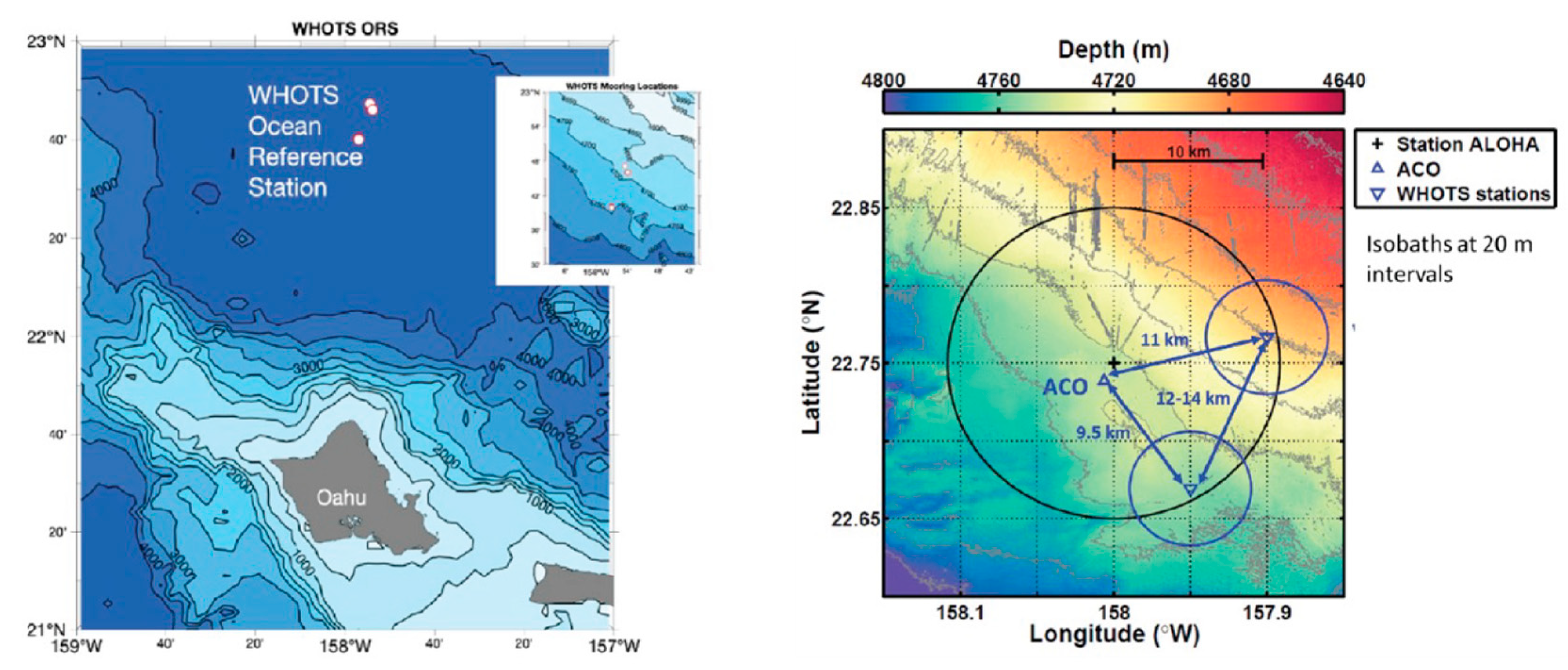
Figure 2.
The WHOTS ORS surface buoy. The anemometers and air temperature and humidity modules (RH/AT) are placed on the upwind side, opposite the vane which carries a radar reflector and satellite transmitter. The cluster of four radiometers, one each for shortwave (DSWR) and longwave (DLWR) from two ASIMET systems, is placed above all other structures. Rain gauges, barometric pressure (BP) sensors are placed aft of the forward face deployed which, with additional stand-alone ASIMET modules, has resulted in 99.5% data completeness of the one-minute records of the meteorological variables except rainfall (the self-siphoning catchment rain gauges are susceptible to biofouling from birds). These time series are of downward shortwave radiation (DSWR), downward longwave radiation (DLWR), air temperature (Ta) and relative (RH) and specific humidity (SH), accumulated precipitation (P) and rain rate (Prate), barometric pressure (SLP), wind speed (WSPD) and direction (WDIR). Sensor heights/depths are included in Table 1. There is no active ventilation of sensors; however, the temperature and humidity sensors are within a multiplate solar radiation shield and the pyrgeometer for DLWR is modified to provide thermopile voltage and body and dome temperature for use with a black-body lab calibration [20], reducing error from solar heating. The post-deployment, calibrated, one-minute records are used to make hourly, daily, monthly, and annual times series.
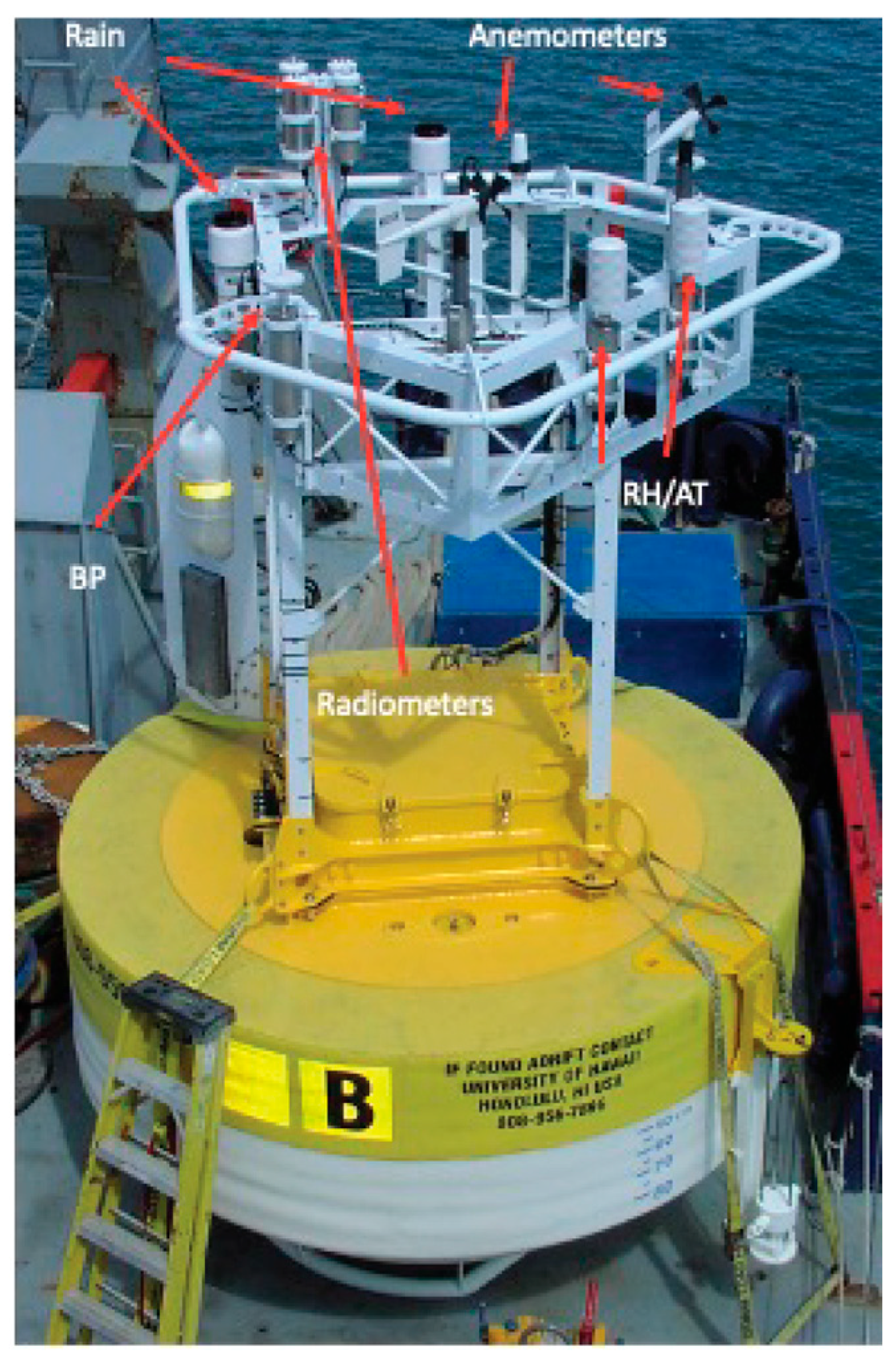
Figure 3.
WHOTS 1 to 17 daily surface meteorology time series from the sensors at the heights as deployed. An additional 20-day smoothing was applied before computing vector wind, and the daily vectors were subsampled every 10 days. The wind records are shown prior to the 2016-2018 gap being filled; the fill is described in Section 1b and subsequent figures use the filled wind record. The rain rate is plotted on a logarithmic scale, and gaps and periods of low rain rate as seen late in 2015 may reflect sensors plugging with guano.
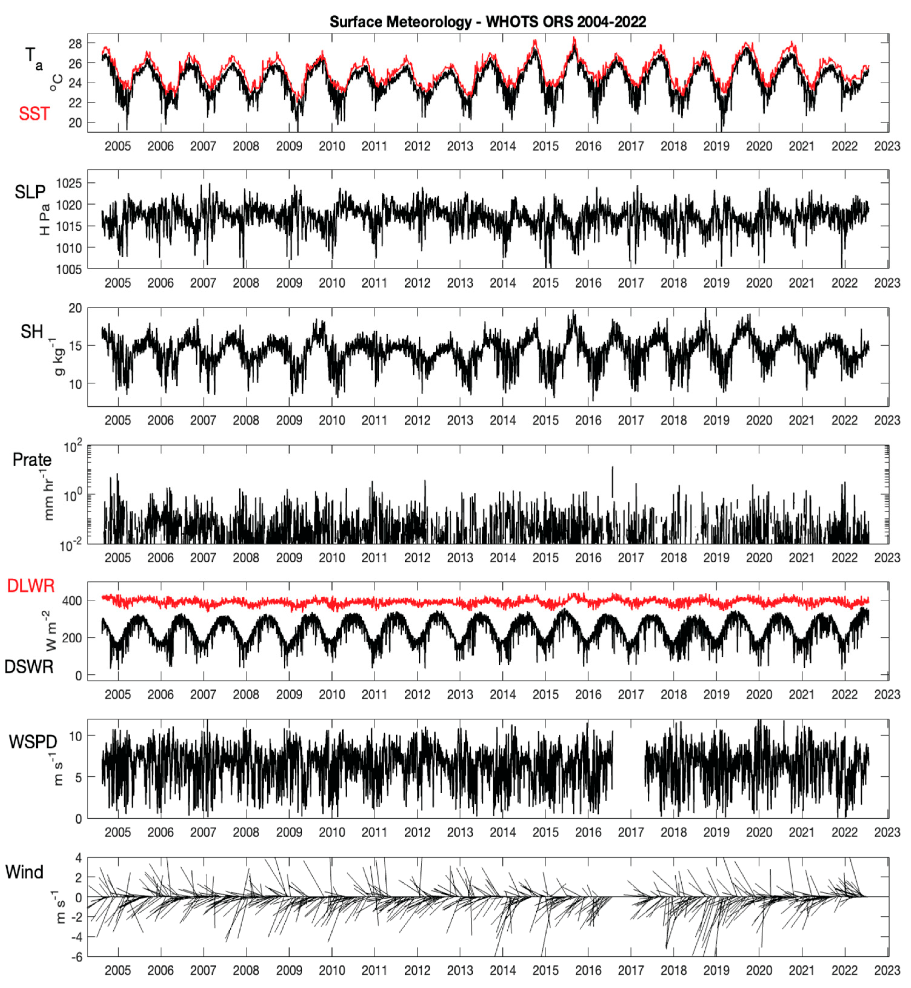
Figure 4.
Histograms of the full length WHOTS 1 to 17 daily surface meteorology as shown in Figure 3 with means and medians indicated. The wind rose for the vector wind shows the direction towards which the wind is blowing, just south of west.
Figure 4.
Histograms of the full length WHOTS 1 to 17 daily surface meteorology as shown in Figure 3 with means and medians indicated. The wind rose for the vector wind shows the direction towards which the wind is blowing, just south of west.
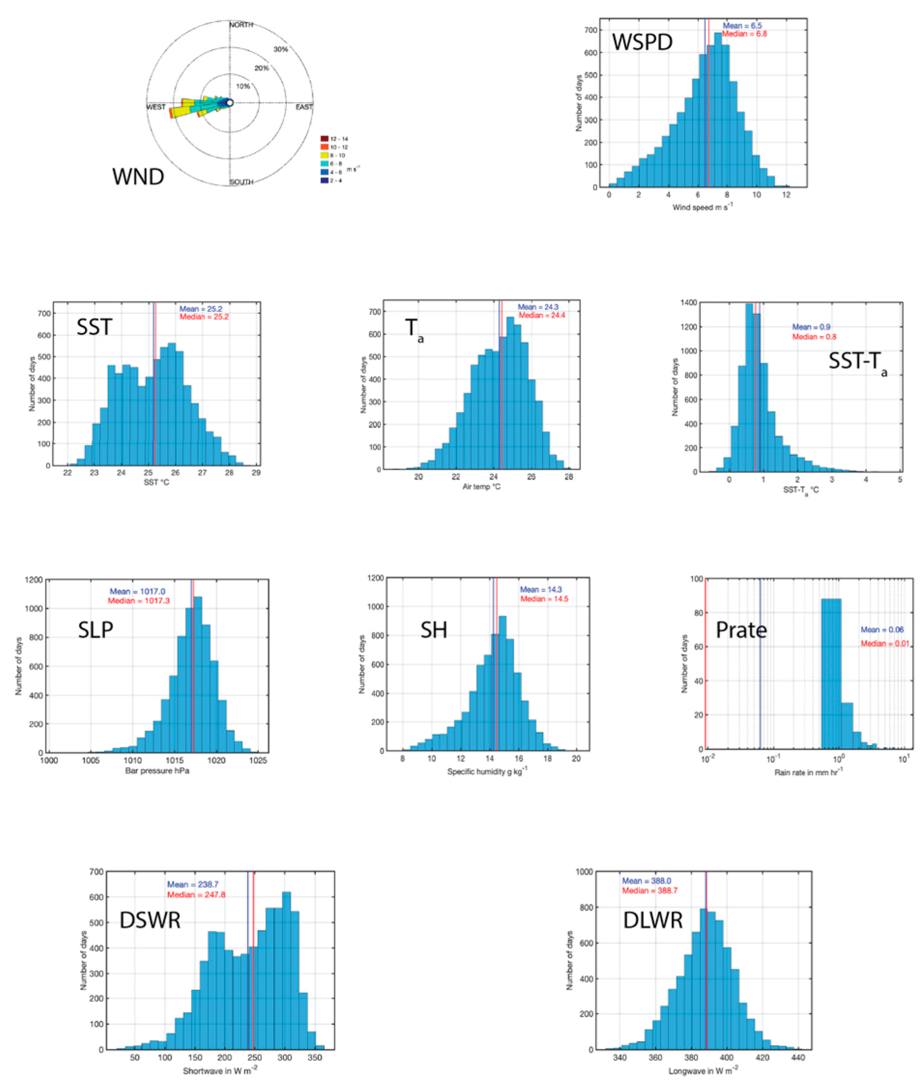
Figure 5.
Time series of daily wind stress magnitude, net het (QN), latent heat (QH), sensible heat (QB), net shortwave (QS), net longwave (QL), and an overplot of rainfall accumulation and cumulative evaporation for WHOTS 1-17. The red line on the QN plot is 10-day smoothing of the black line for daily QN. Wind stress time series is based on the gap-filled wind time series.
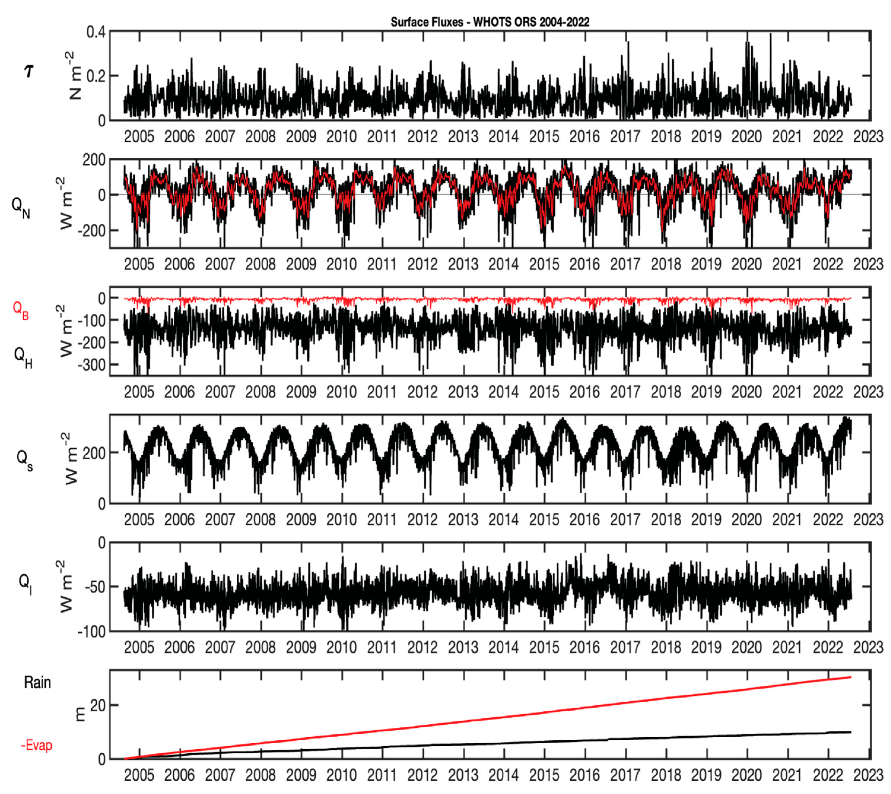
Figure 6.
Histograms of the daily averaged wind stress magnitude (|τ|), net heat flux (QN), net shortwave (Qs), net longwave radiation (Ql), latent heat flux (QH), and sensible heat flux (QB), with mean and medians indicated. The full-length time series were used, including fractional years.
Figure 6.
Histograms of the daily averaged wind stress magnitude (|τ|), net heat flux (QN), net shortwave (Qs), net longwave radiation (Ql), latent heat flux (QH), and sensible heat flux (QB), with mean and medians indicated. The full-length time series were used, including fractional years.
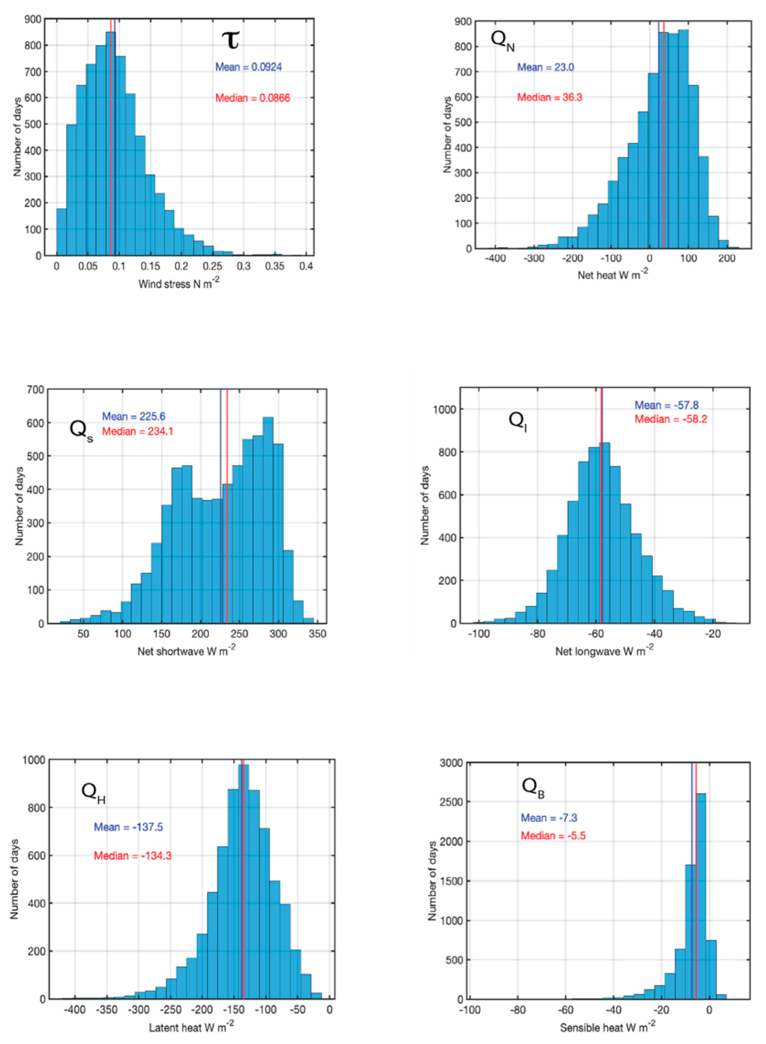
Figure 7.
Frequency spectra computed using one-minute WHOTS ORS time series of Qs, QH, and SLP from calendar year 2009. Band-averaging increases with frequency and the 95% confidence limits shown for the spectral levels reflect the band-averaging.
Figure 7.
Frequency spectra computed using one-minute WHOTS ORS time series of Qs, QH, and SLP from calendar year 2009. Band-averaging increases with frequency and the 95% confidence limits shown for the spectral levels reflect the band-averaging.
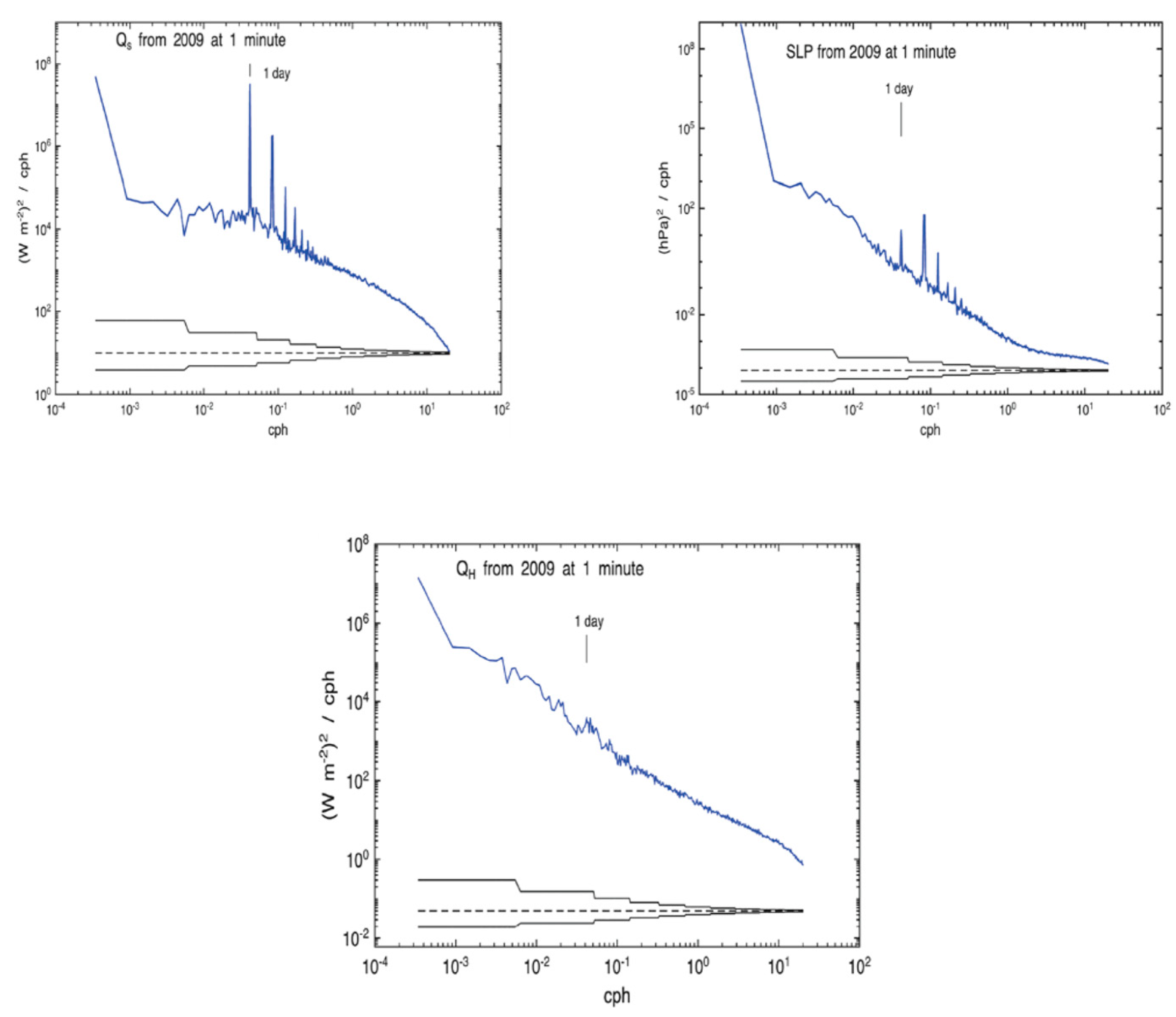
Figure 8.
One-minute time series of DSWR, QN, SST, and the rate of change dSST/dt from May 6-7, 2020 with time base in hours UTC. An estimate of the clear sky DSWR is overplotted in red over the with observed DSWR. The record maxima in DSWR contribute to record maxima in QN, and the SST and dSST/dt time series show response to transient high values in QN. This will be referred to as the “High sun” event.
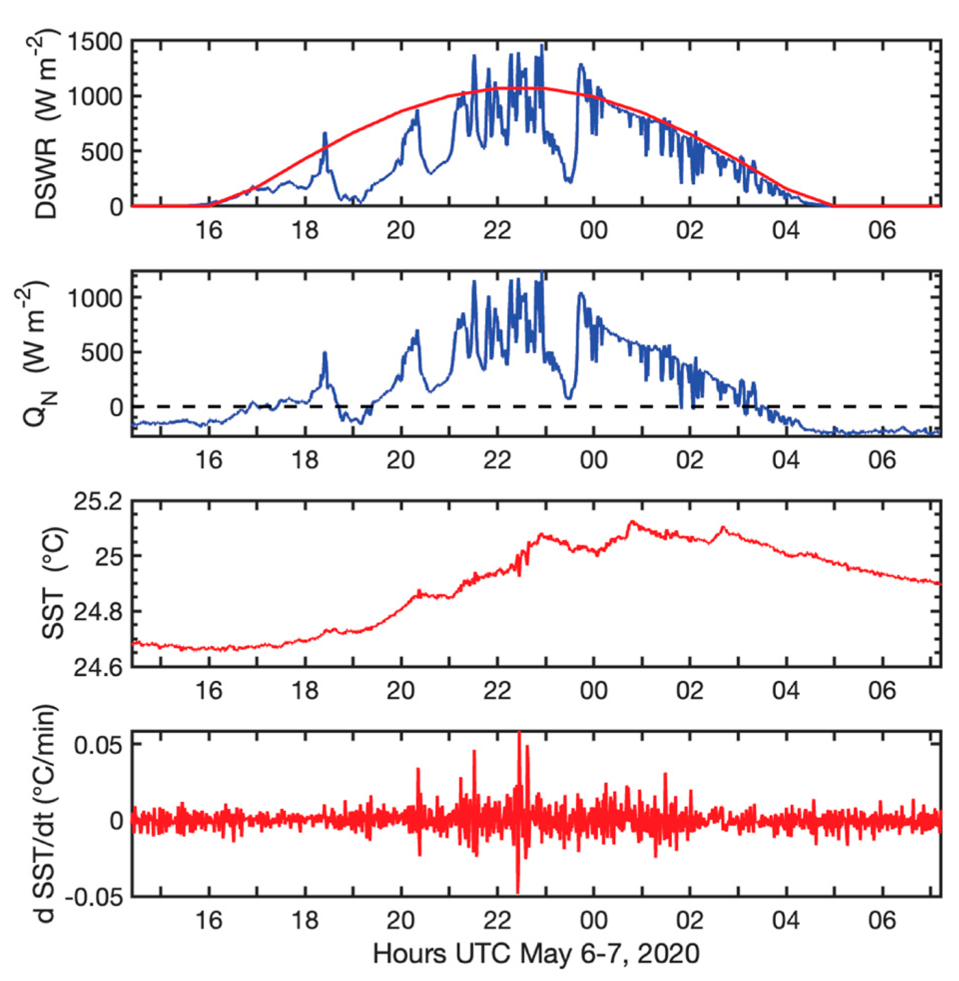
Figure 9.
One-minute time series of SST, WSPD, QN, and QH beginning on September 5, 2017 (UTC), spanning September 6, and including the first 12 h of September 7, 2017. The time base is in hours UTC. The record maximum in SST occurring early on September 7 coincident with a period of low winds, cloud-free skies, and reduced latent heat loss. This is called “Low wind 1”.
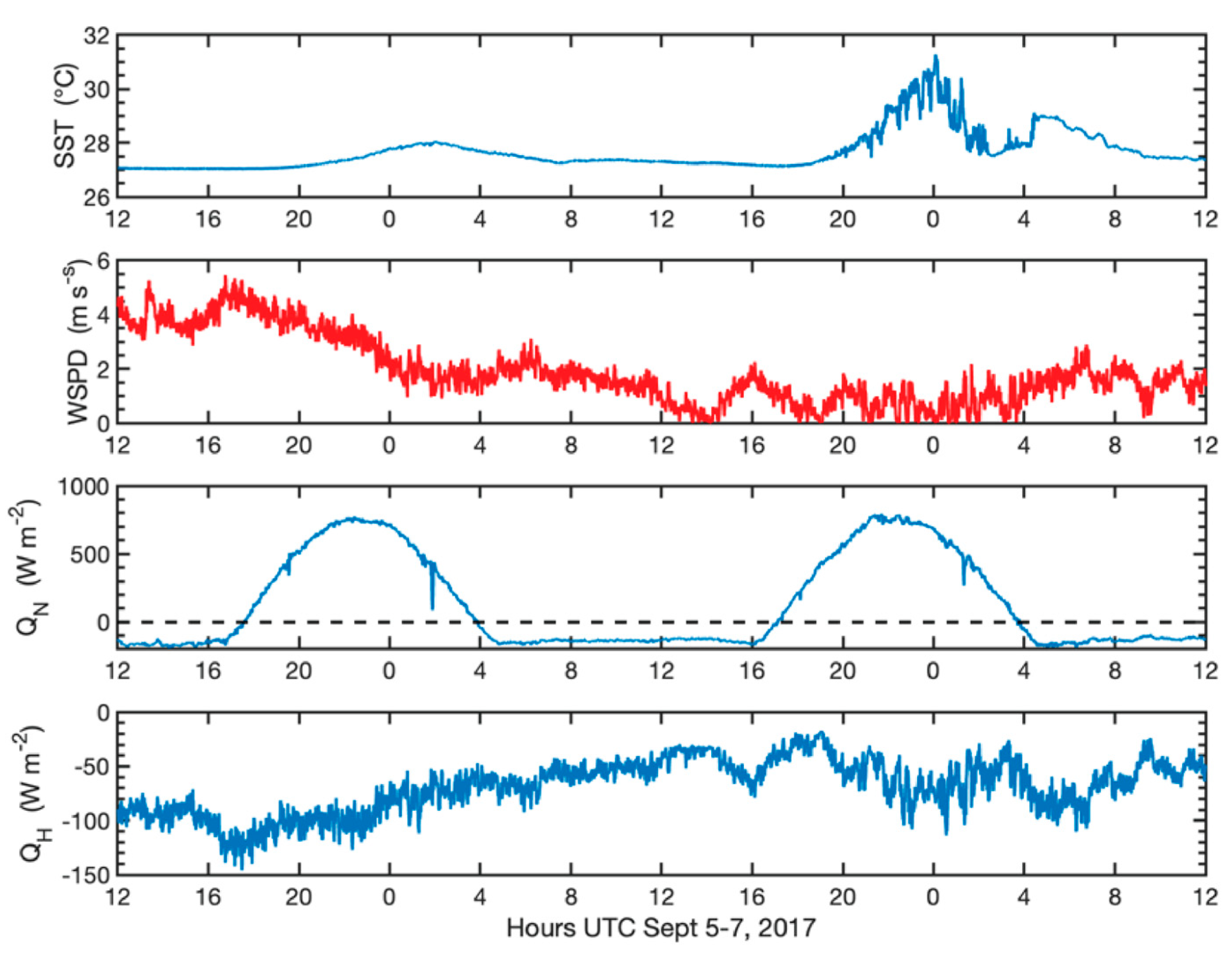
Figure 10.
One-minute Ta, QB, WSPD. Prate, and Qs from February 10, 2019 UTC, when the record minima in Ta (15.89 °C) and in QB (-192.0 W m−2) were observed. The time axis is in hours UTC. The event is referred to as “Downdrafts”.
Figure 10.
One-minute Ta, QB, WSPD. Prate, and Qs from February 10, 2019 UTC, when the record minima in Ta (15.89 °C) and in QB (-192.0 W m−2) were observed. The time axis is in hours UTC. The event is referred to as “Downdrafts”.
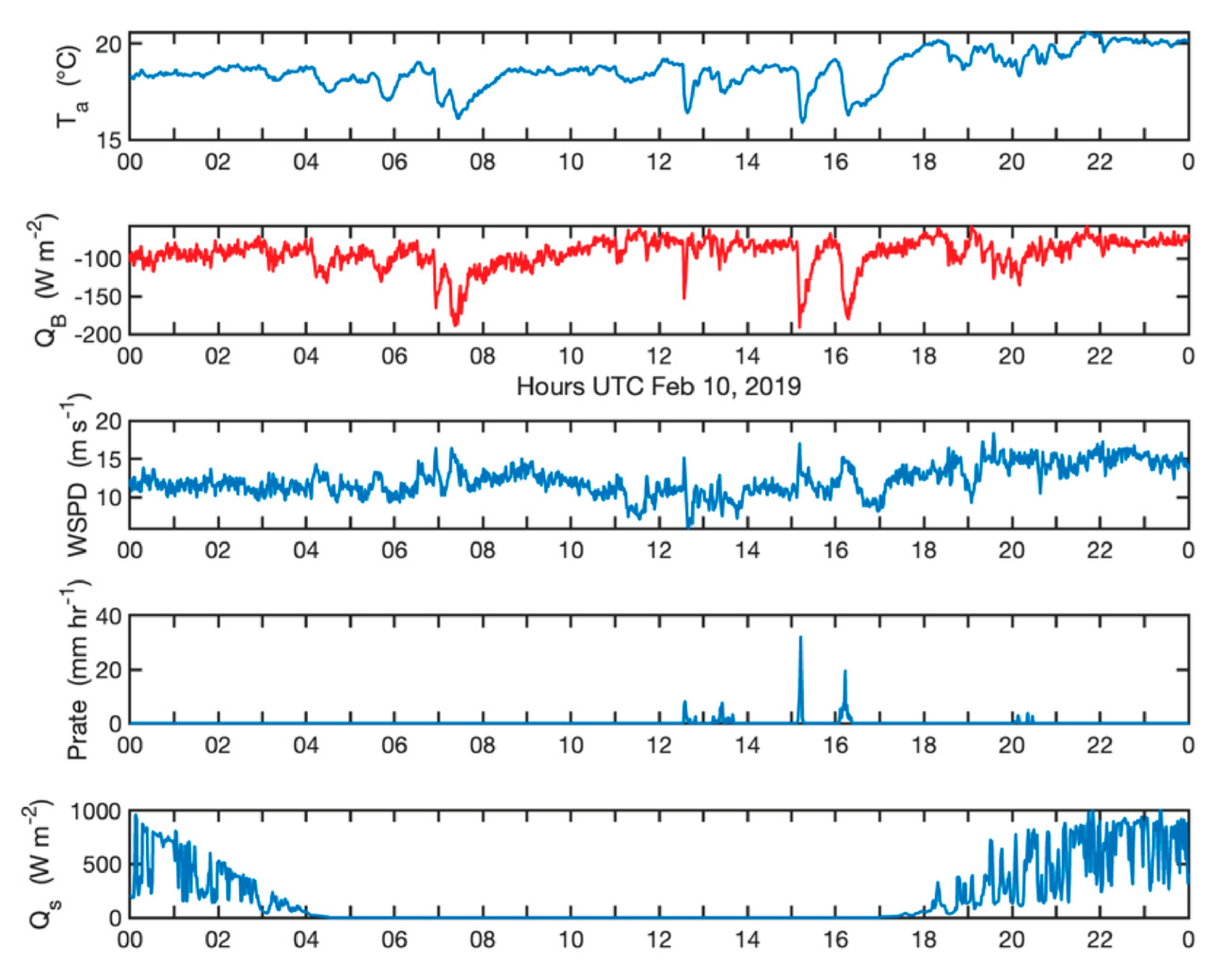
Figure 11.
One-minute time series of SH, WSPD, QH, Ql, and QN from February 10-12, 2019, when minima in QH, Ql, and QN were observed; referred to as “Dry air” event. The time axis shows day of month/hour UTC.
Figure 11.
One-minute time series of SH, WSPD, QH, Ql, and QN from February 10-12, 2019, when minima in QH, Ql, and QN were observed; referred to as “Dry air” event. The time axis shows day of month/hour UTC.
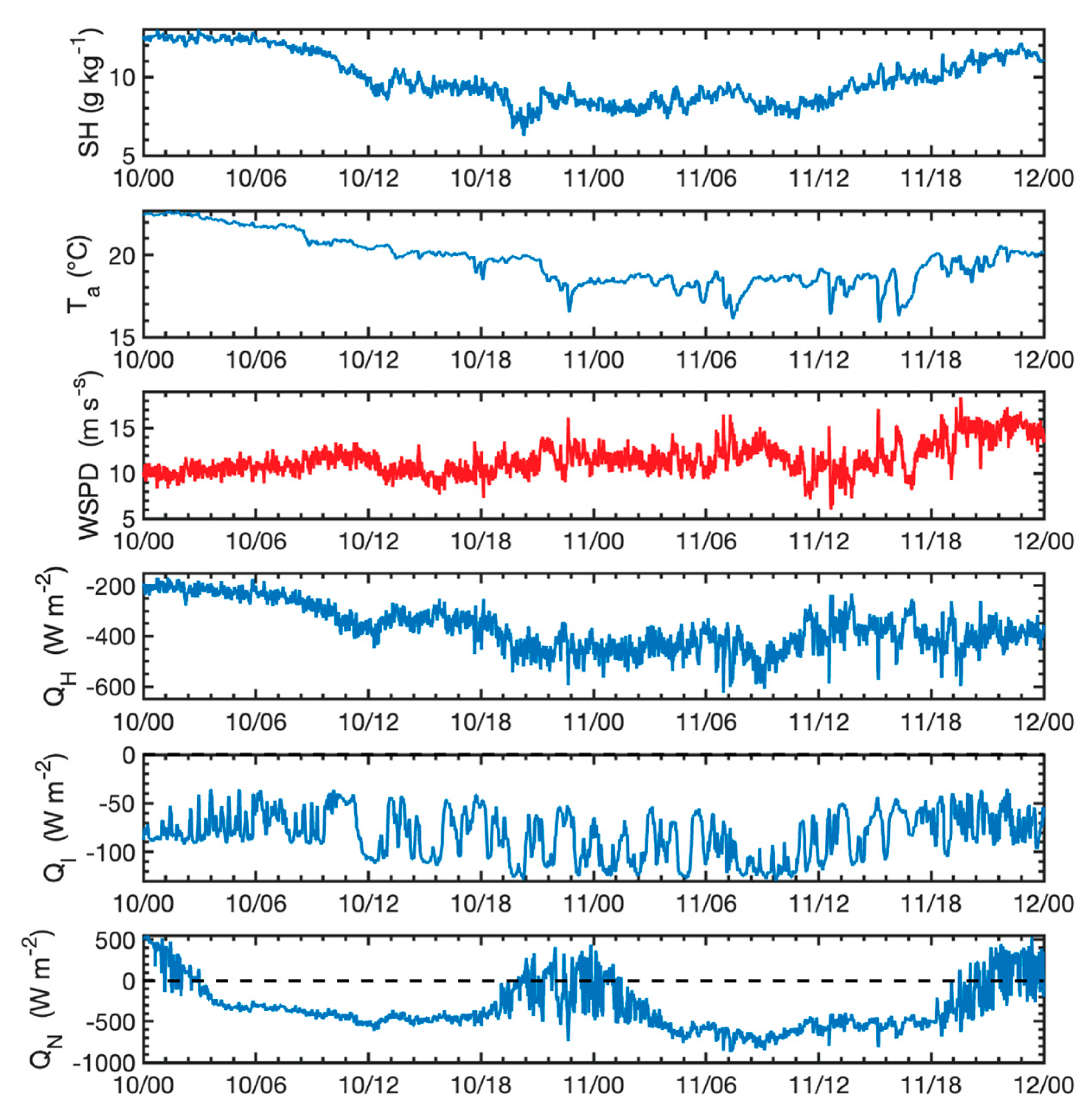
Figure 12.
a. Surface meteorology for strong, transient warm event (‘TWE’) in Ta on January 16, 2011. Ta, SST, specific humidity at 2m, WSPD, WNDE and WNDN, DSWR, PRATE, and SLP sampled at one-minute air plotted here, with wind stress magnitude, QN, Qs, Ql, QH, and QB plotted in Figure 11b. The time axis is in hours UTC on January 16, 2011.
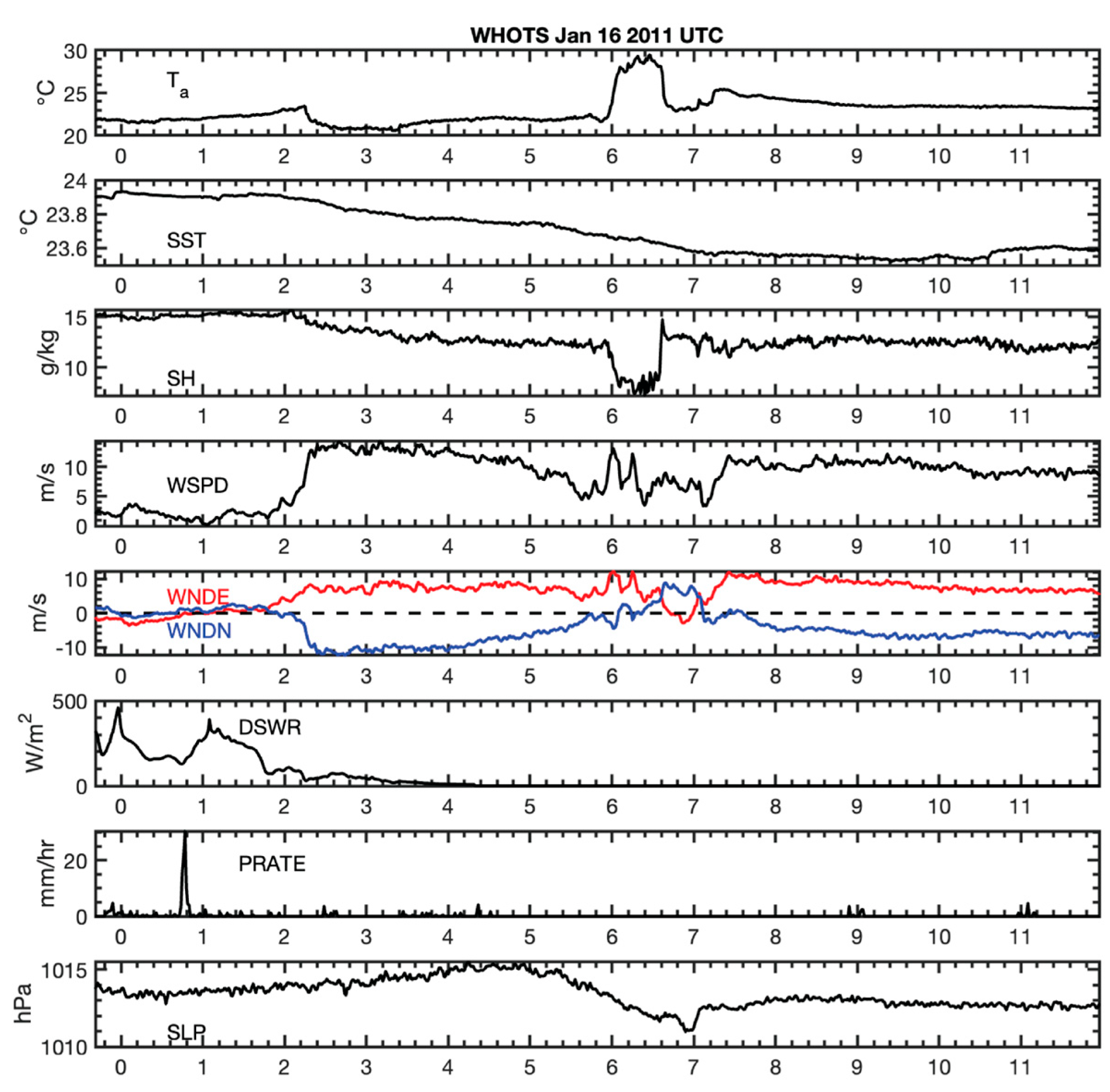
Figure 12.
b. Surface fluxes for strong, transient warm event (‘TWE’) in Ta on January 16, 2011. Wind stress magnitude, QN, Qs, Ql, QH, and QB plotted with time axis is in hours UTC on January 16, 2011.
Figure 12.
b. Surface fluxes for strong, transient warm event (‘TWE’) in Ta on January 16, 2011. Wind stress magnitude, QN, Qs, Ql, QH, and QB plotted with time axis is in hours UTC on January 16, 2011.
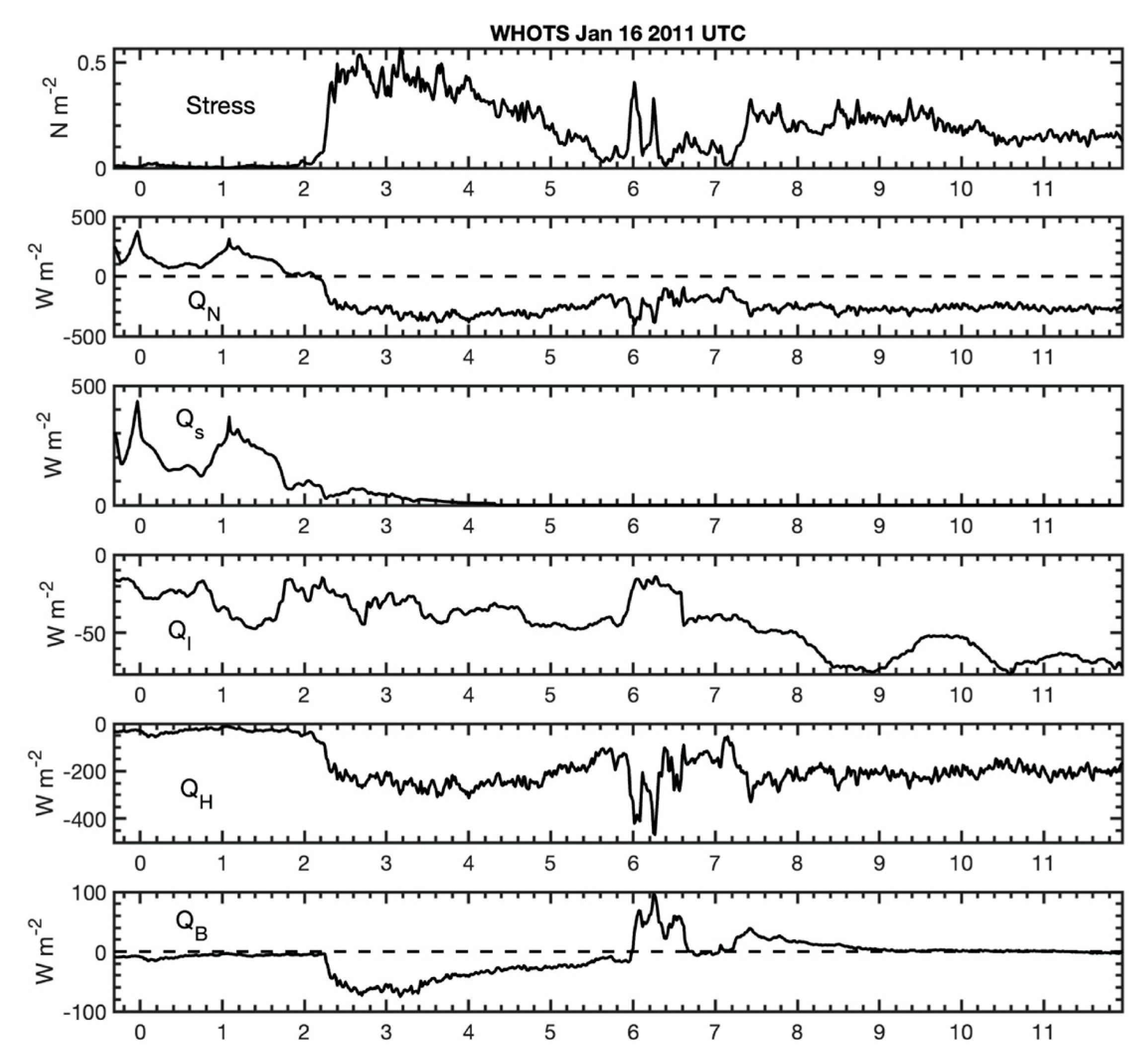
Figure 13.
One-minute time series of PRATE, heat loss due to rain, Qr, surface salinity, SST, and SLP for the period referred to as “Rain event” on December 1 to 2, 2013. The time axis is in days of the month/hours UTC.
Figure 13.
One-minute time series of PRATE, heat loss due to rain, Qr, surface salinity, SST, and SLP for the period referred to as “Rain event” on December 1 to 2, 2013. The time axis is in days of the month/hours UTC.
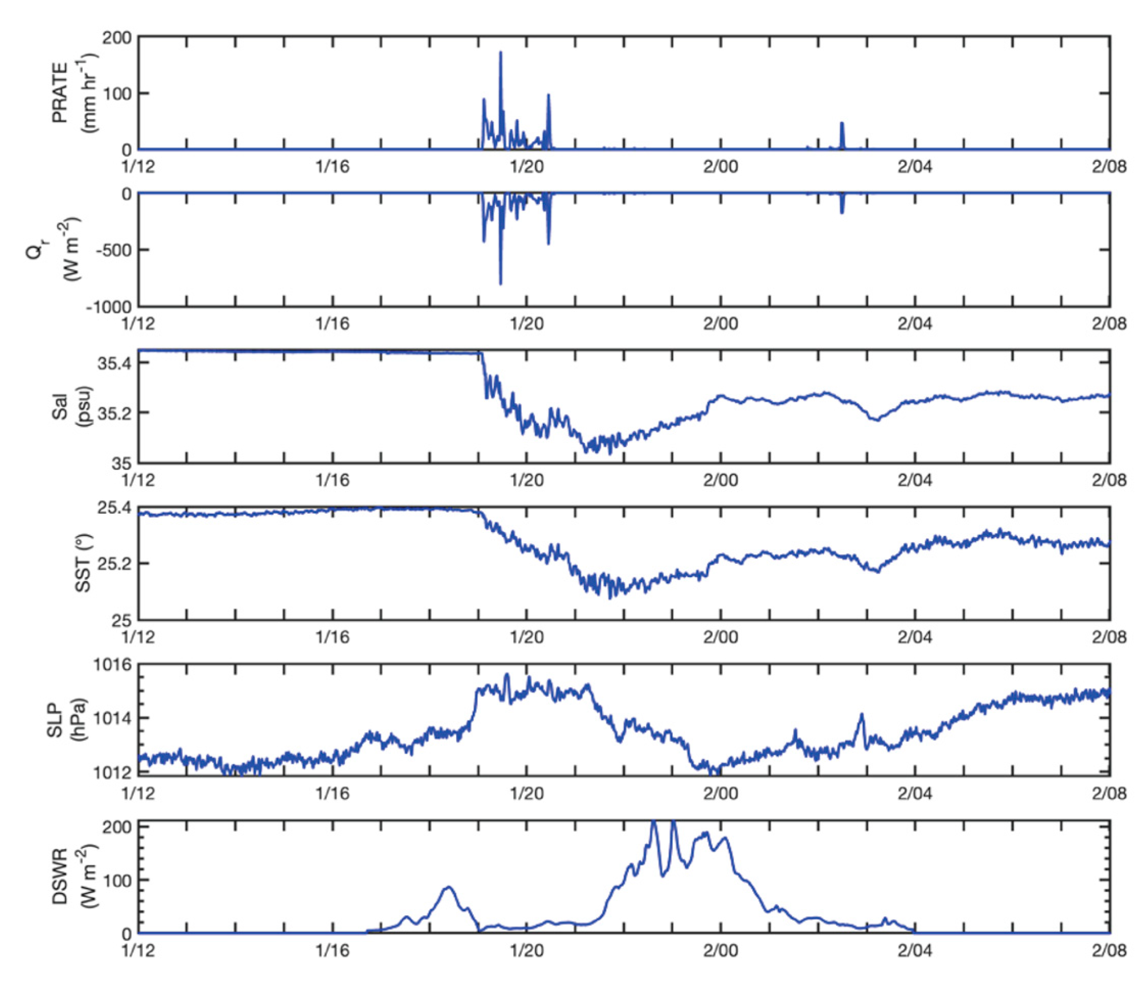
Figure 14.
One-minute time series from July 26-27, 2020 (HST). Wind stress magnitude, WSPD, Wdir, PRATE, SLP, and QN show the signatures of the passage of Hurricane Douglas close to WHOTS. This event referred to as “Douglas 1”. The time axis is in hours local Hawaii Standard Time to ease comparison with local reports, where HST=UTC-10.
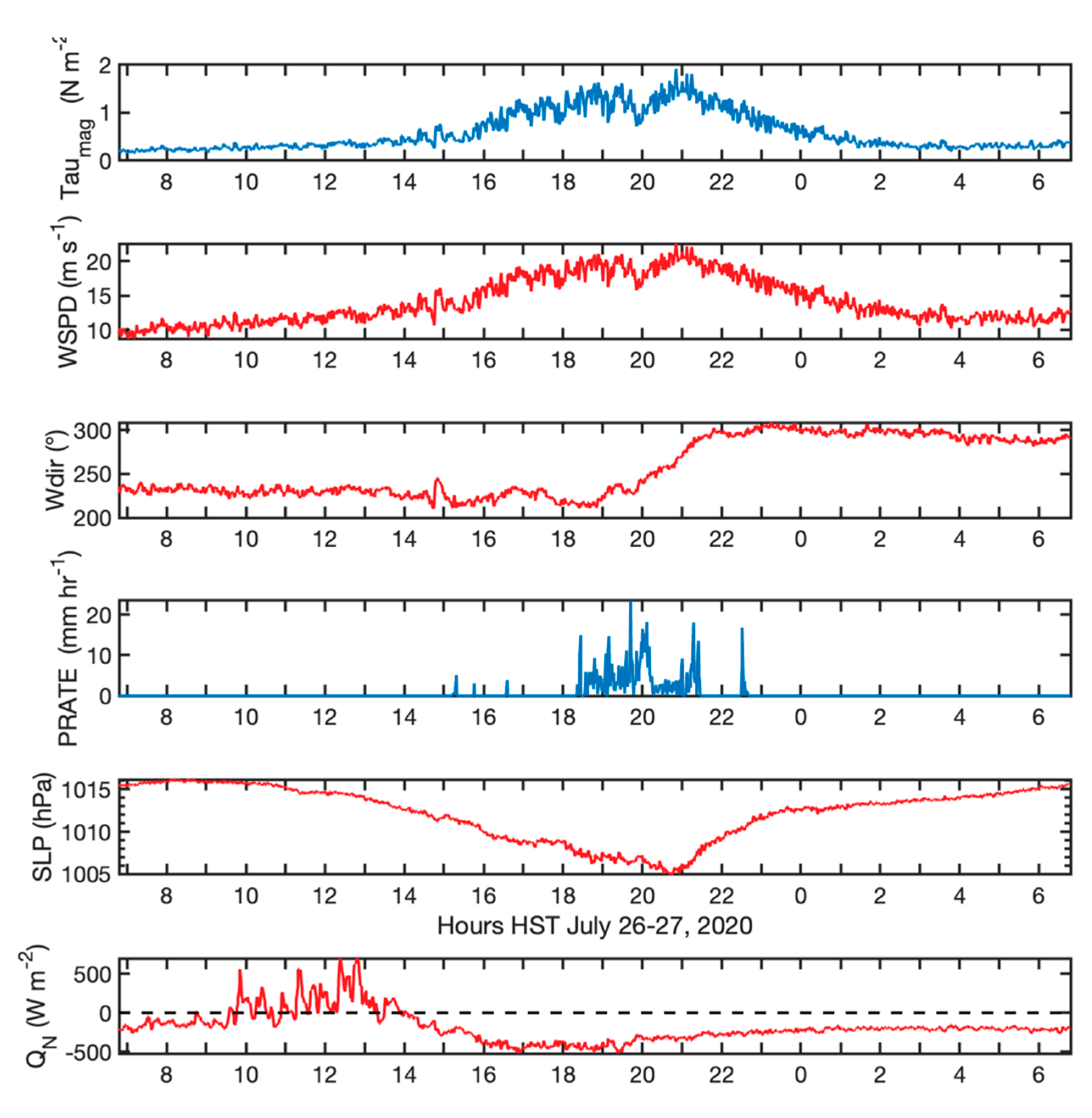
Figure 15.
Daily mean cycles computed from the hourly time series from 2005 to 2021 inclusive. Years 2016 and 2017 were not complete for wind and excluded. The shaded vertical bar spans the times of local solar noon over each year. Both the scalar wind speed (one hour average of one-minute speeds) and vector wind speed (one hour vector average of one-minute winds) are shown. Wind direction is degrees towards.
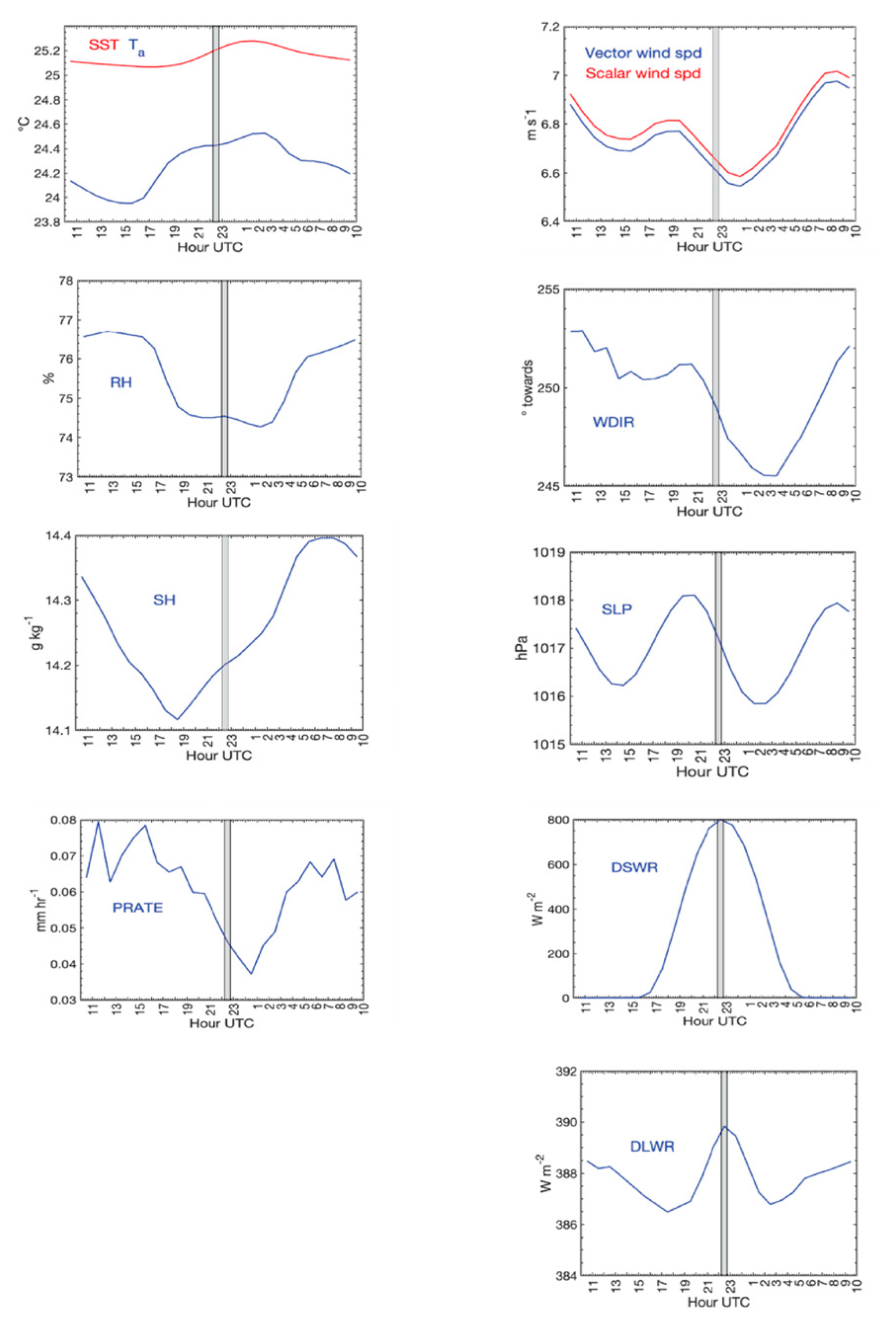
Figure 16.
The mean daily cycle in heat fluxes and wind stress for years 2005 to 2021 inclusive, excepting 2016 and 2017 in the wind stress daily means cycle. Wind stress magnitude computed using both one-minute velocities and one-hour vector-averaged wind velocities are shown. Stress direction is towards.
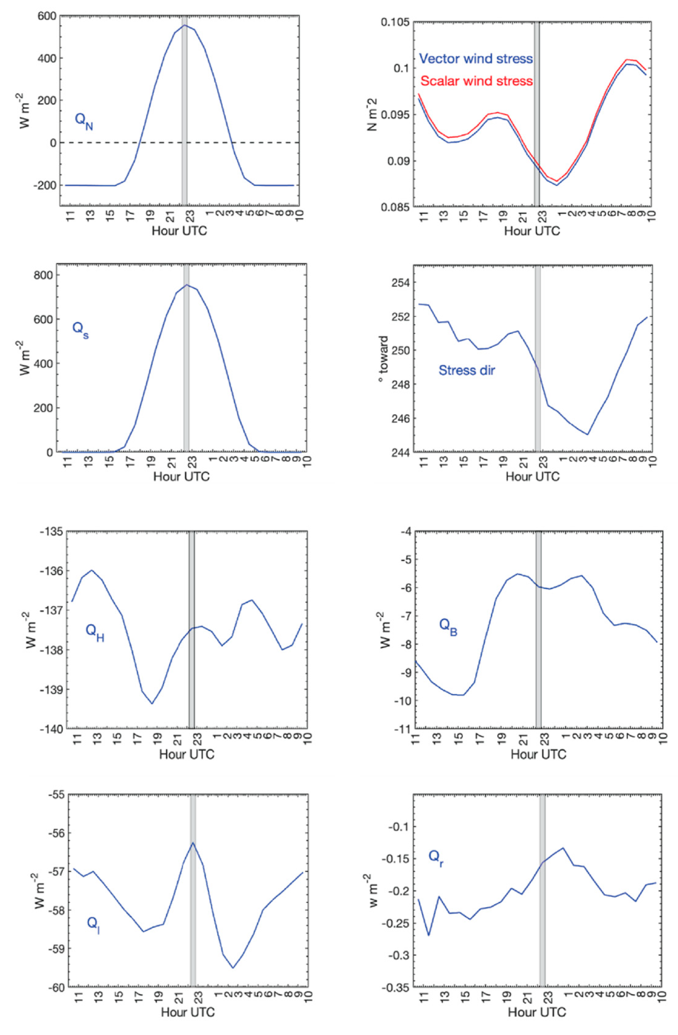
Figure 17.
Time series of hourly surface meteorology and air-sea fluxes October 6 to 21, 2009, referred to as “Low wind 2”. Surface meteorology includes Ta, SST, SLP, SH, Prate, DSWR, DLWR, and WSPD. WSPD drops during October 8-11 and again October 16-17. Air sea flux plots include wind stress magnitude, QN, QH, QB, QS, and Ql. Below the fluxes are an overplot of accumulated rainfall and evaporation and a plot of time integrated air-sea heat flux. X axis shows days of October 2009 UTC.
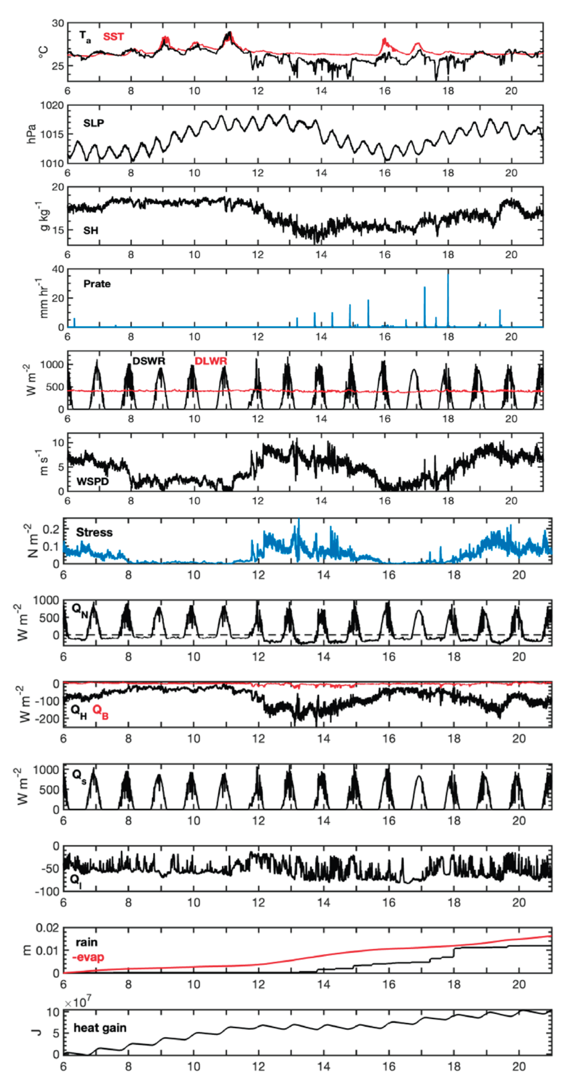
Figure 18.
Time series of hourly surface meteorology and air-sea fluxes November 9 to December 19, 2012. Surface meteorology includes Ta, SST, SLP, SH, Prate, DSWR, DLWR, and WSPD. SH drops during November 16 and again November 27-29. Air-sea flux plots include wind stress magnitude, QN, QH, QB, QS, and Ql. Below the fluxes are an overplot of cumulative rainfall and evaporation and a plot of cumulative air-sea heat flux. X axis shows days of November-December; event referred to as “Heat loss 1.).
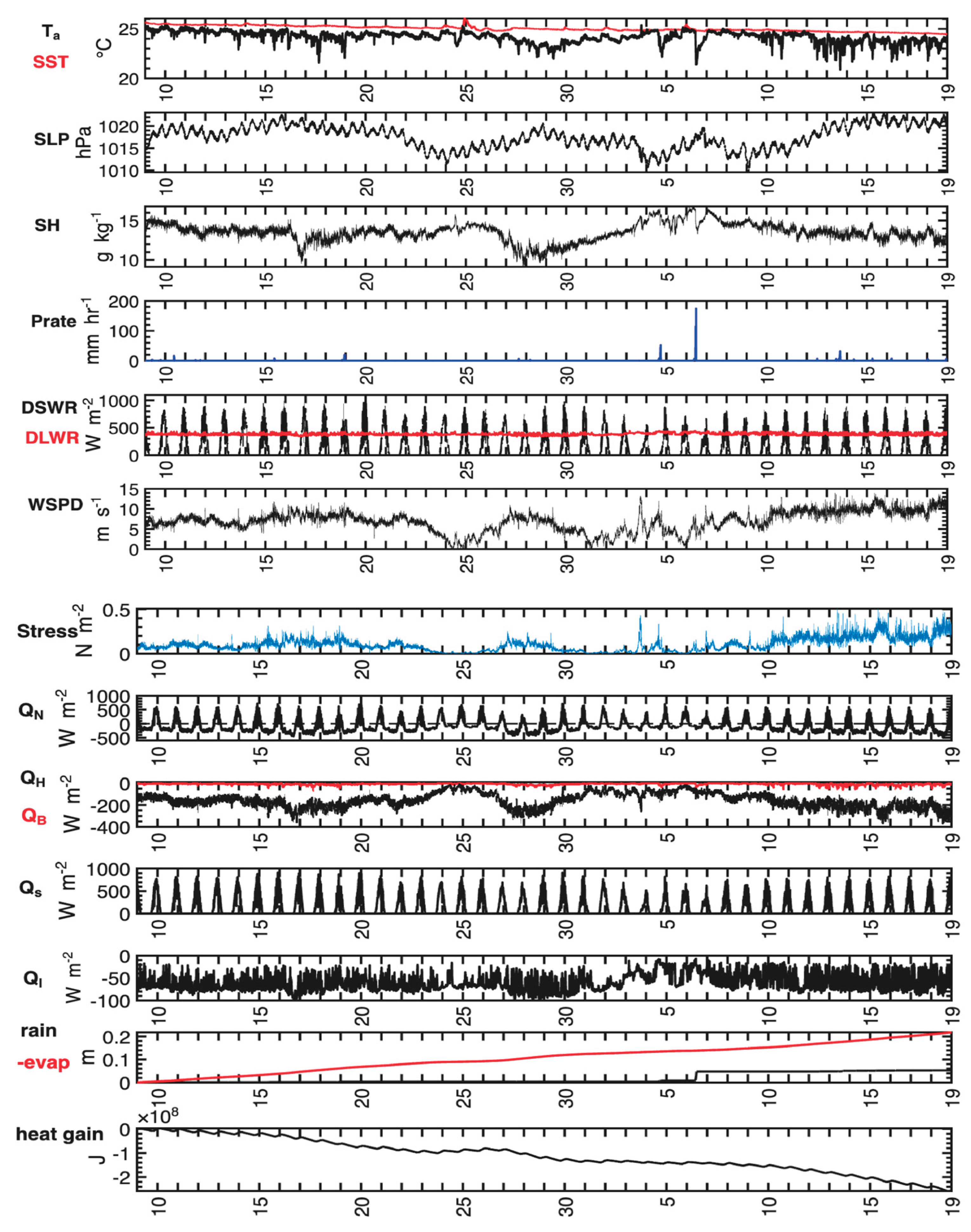
Figure 19.
Time series of hourly surface meteorology and air-sea fluxes January 9 to February 28, 2010 (Heat loss 2). Below the fluxes are an overplot of time integrated rainfall and evaporation and a plot of time integrated air-sea heat flux. X axis shows days of January into February UTC.
Figure 19.
Time series of hourly surface meteorology and air-sea fluxes January 9 to February 28, 2010 (Heat loss 2). Below the fluxes are an overplot of time integrated rainfall and evaporation and a plot of time integrated air-sea heat flux. X axis shows days of January into February UTC.
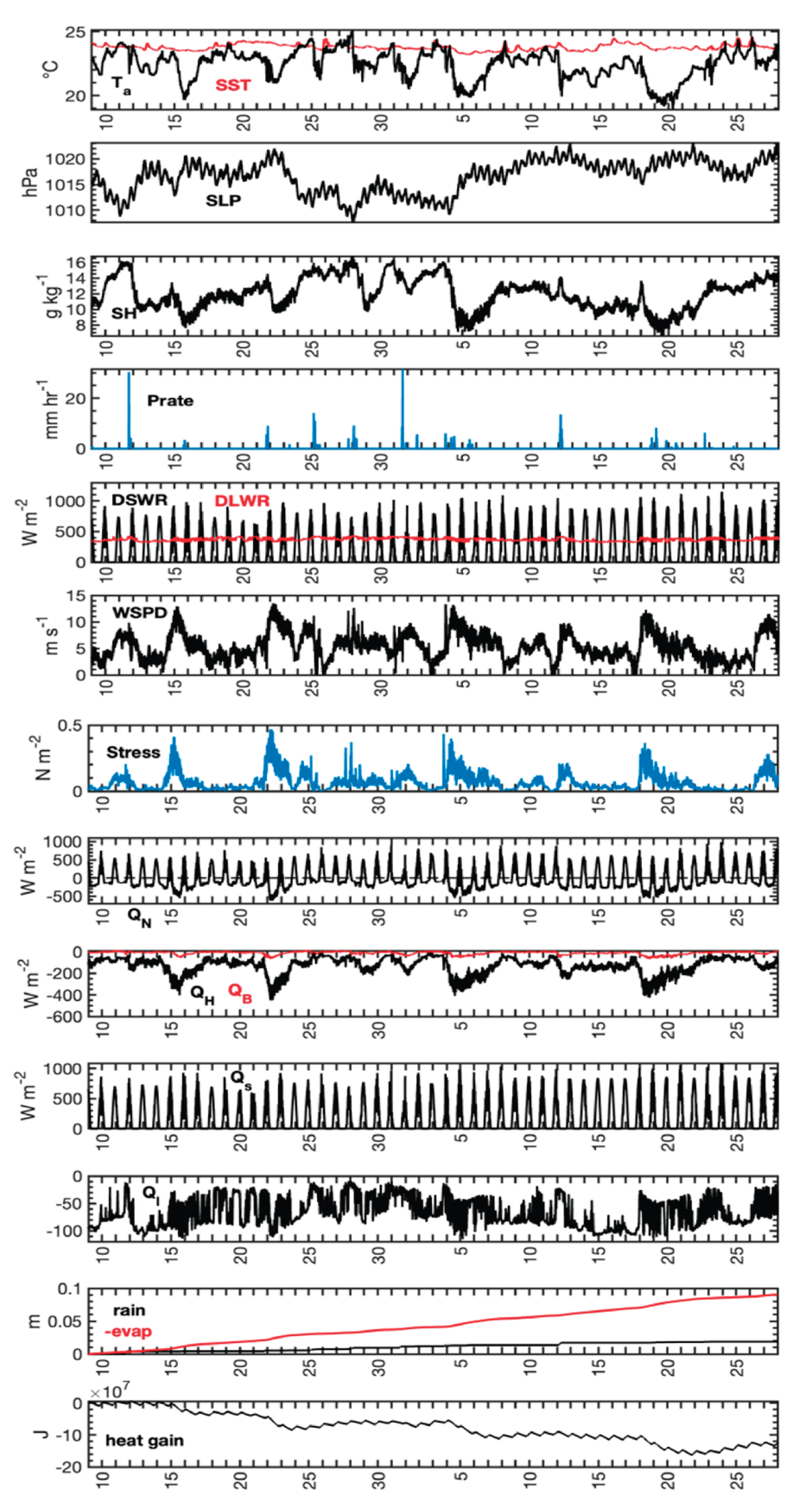
Figure 20.
Time series of hourly surface meteorology and air-sea fluxes July 10 to 28, 2016 during Hurricane Darby. Below the fluxes are an overplot of cumulative rainfall and evaporation and a plot of cumulative air-sea heat flux. X axis shows days of July (UTC).
Figure 20.
Time series of hourly surface meteorology and air-sea fluxes July 10 to 28, 2016 during Hurricane Darby. Below the fluxes are an overplot of cumulative rainfall and evaporation and a plot of cumulative air-sea heat flux. X axis shows days of July (UTC).
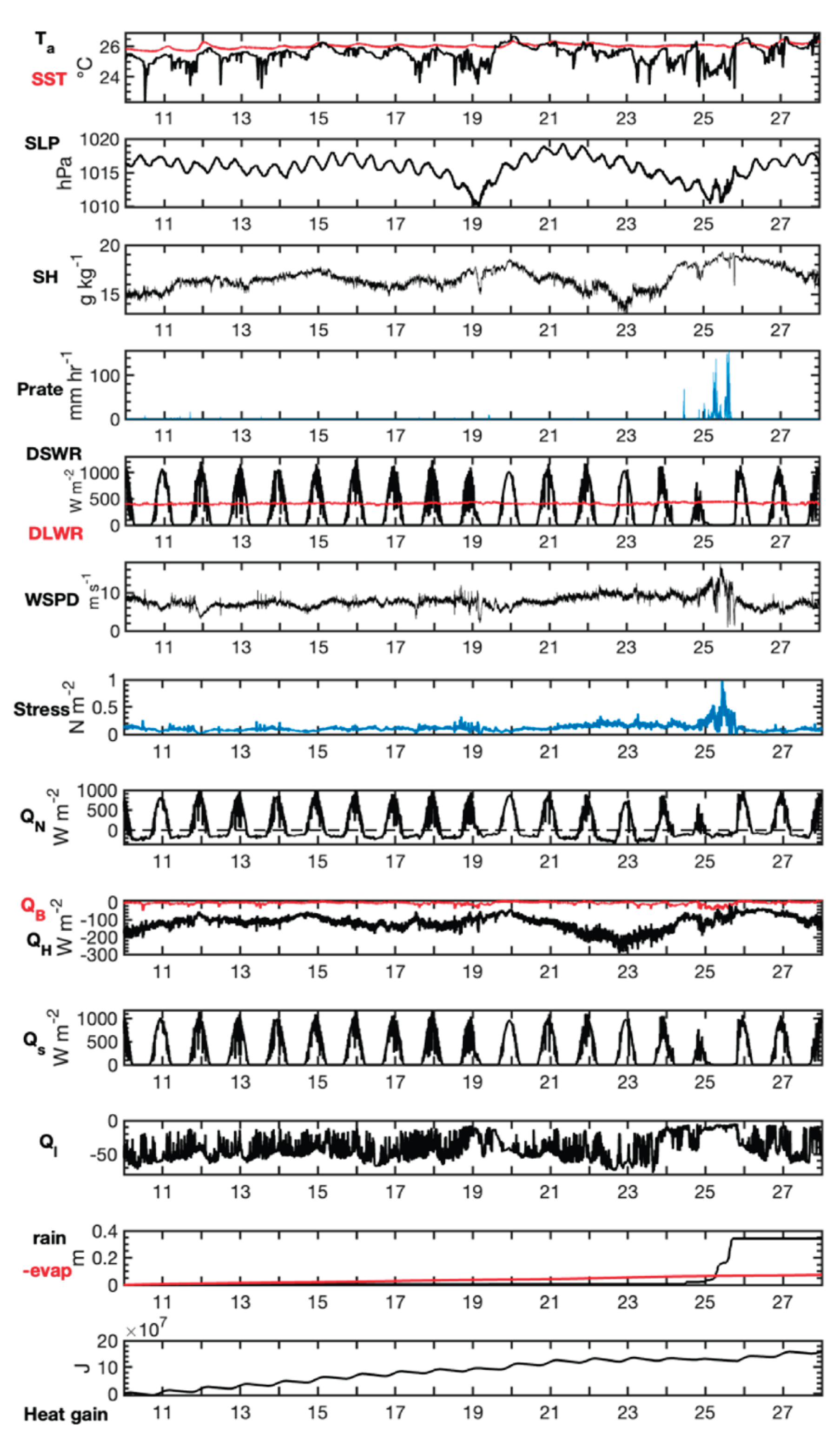
Figure 21.
Time series of hourly surface meteorology and air-sea fluxes July 20 to 30, 2020 during Hurricane Douglas (‘Douglas 2’). Below the fluxes are an overplot of cumulative rainfall and evaporation and a plot of cumulative air-sea heat flux. X axis shows days of July UTC.
Figure 21.
Time series of hourly surface meteorology and air-sea fluxes July 20 to 30, 2020 during Hurricane Douglas (‘Douglas 2’). Below the fluxes are an overplot of cumulative rainfall and evaporation and a plot of cumulative air-sea heat flux. X axis shows days of July UTC.
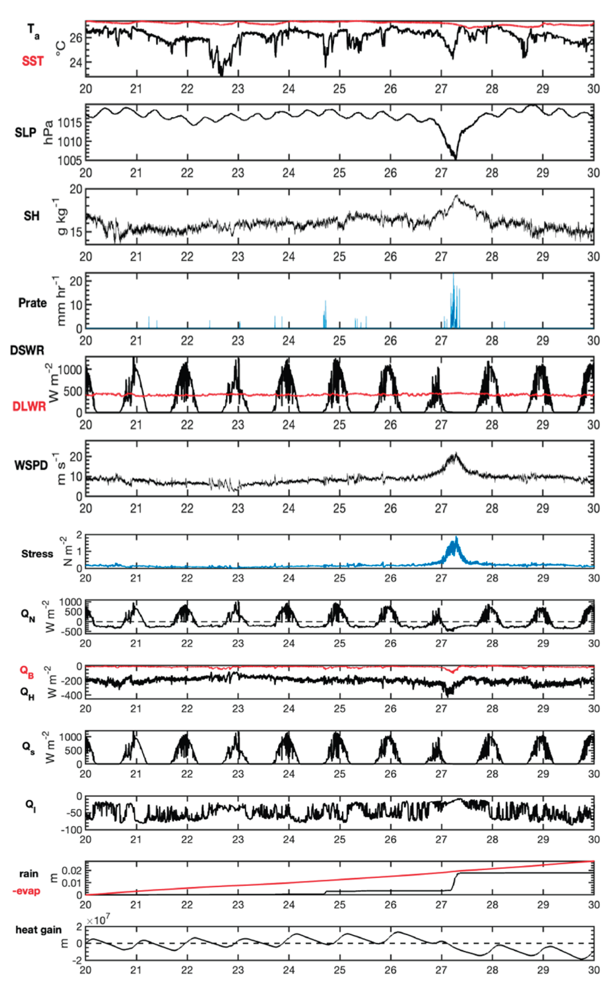
Figure 22.
Mean annual cycle of daily averaged surface meteorology for WHOTS 1-17, plotted as daily time series. Wind direction is direction towards.
Figure 22.
Mean annual cycle of daily averaged surface meteorology for WHOTS 1-17, plotted as daily time series. Wind direction is direction towards.
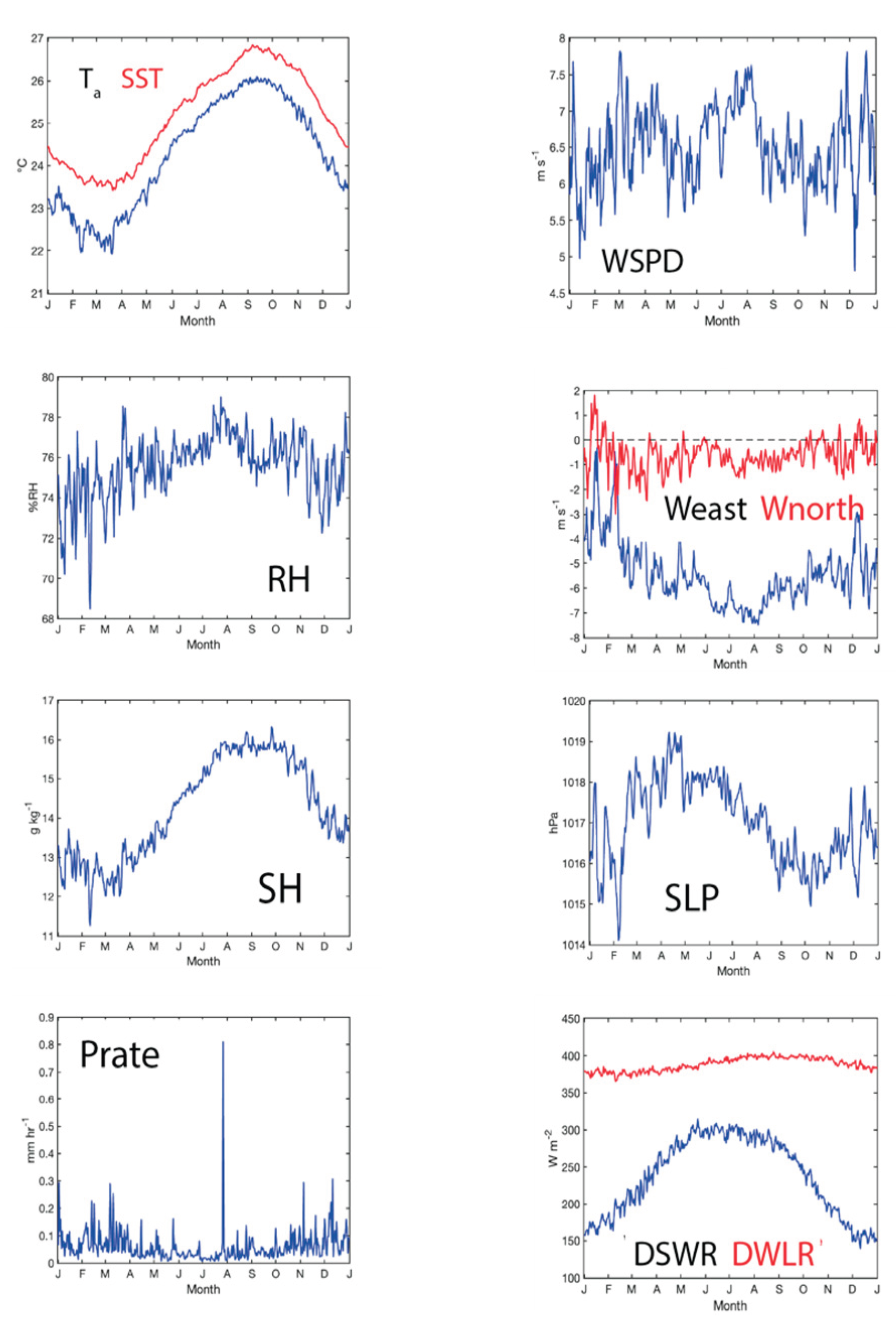
Figure 23.
Mean annual cycles of the wind stress, the neat heat flux, and the heat flux components.
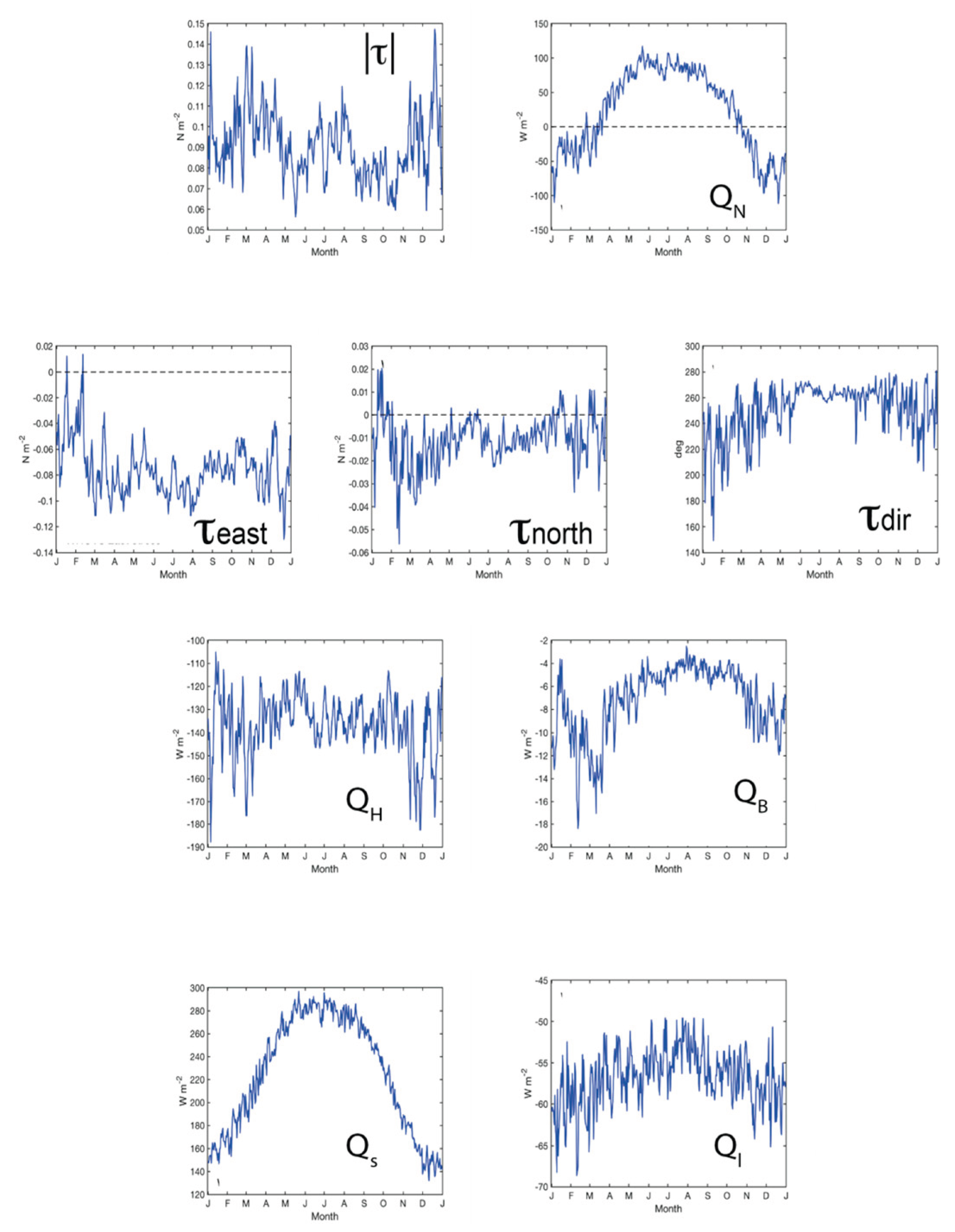
Figure 24.
Annual summary of cumulative net heat gain and freshwater flux together with accumulating rainfall and evaporation.
Figure 24.
Annual summary of cumulative net heat gain and freshwater flux together with accumulating rainfall and evaporation.
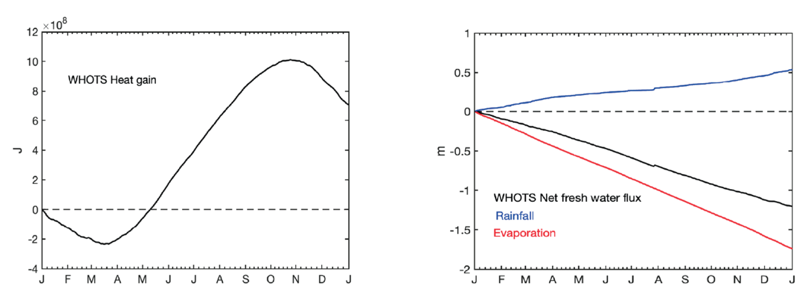
Figure 25.
The event totalized heat, freshwater, and mechanical energy gains normalized by event duration to yield mean gain per day during each event type.
Figure 25.
The event totalized heat, freshwater, and mechanical energy gains normalized by event duration to yield mean gain per day during each event type.
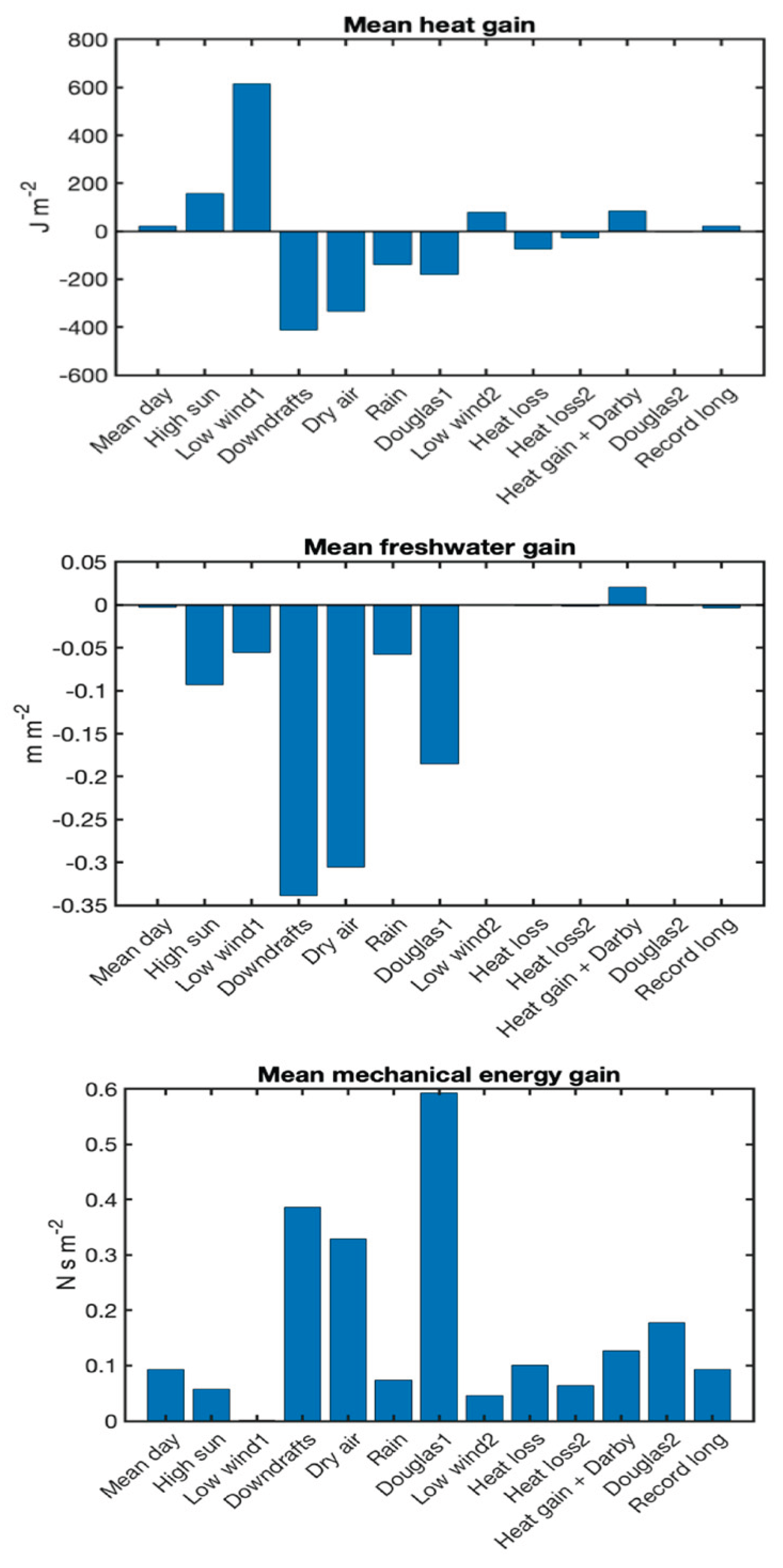
Table 3.
Uncertainties of annual averaged fluxes from an ORS buoy, after Colbo and Weller [14] and Weller [23]. The accuracy of the freshwater flux (E-Prate) was calculated computing evaporation (E) from latent heat flux and observed rainfall (Prate) at the WHOTS ORS. Uncertainty in QR stems from uncertainty in the rain rate. WHOTS 1-17 long-term mean values provide a context for the uncertainties. Except for wind stress and freshwater flux rate, all are means of January 1, 2005 to December 31, 2021. Mean stress direction is based on the mean stress components.
| Flux | WHOTS mean | One-minute | Daily | Annual |
|---|---|---|---|---|
| Net longwave (QL,W m−2) | -57.0 | 7.5 | 2 | 2 |
| Net shortwave (QS, W m−2) | 225.0 | 10 | 3 | 3 |
| Latent (QH, W m−2) | -137.5 | 5 | 4 | 4 |
| Sensible (QB, W m−2) | -7.3 | 1.5 | 1.5 | 1.5 |
| Rain heat flux (QR, W m−2) | -0.2 | 10% | 10% | 10% |
| Net heat flux (QN, W m−2) | 23.2 | 15 | 8 | 8 |
| Wind stress magnitude (τ, N m−2) | 0.0938 | .007 | .007 | .007 |
| East wind stress (τE, N m−2) | -0.0762 | .007 | .007 | .007 |
| North wind stress (τN, N m−2) | -0.0115 | .007 | .007 | .007 |
| Wind stress direction (τdir, °) | 261.4 | 6 | 5 | 5 |
| E-P (mm hr−1) | -0.14 | 10% | 10% | 10% |
Table 4.
Means, minima, and maxima for full calendar years 2005 to 2021 inclusive. Minima and maxima are shown from 1-min, 1-h, and 1-day time series. The height adjusted air temperature and specific humidity (to 2 m), wind (to 10 m), and ocean skin temperature are also given, along with delta T (skin temperature from the COARE algorithm minus the 2 m Ta). Wind and ocean current directions are towards.
| Mean | Min | Max | |||||
|---|---|---|---|---|---|---|---|
| 1-min | 1-h | 1-day | 1-min | 1-h | 1-day | ||
| obs Ta (°C) | 24.26 | 15.89 | 16.95 | 18.62 | 29.54 | 29.17 | 27.96 |
| 2m Ta (°C) | 24.31 | 16.14 | 17.17 | 18.79 | 29.65 | 29.21 | 27.99 |
| obs SST (°C) | 25.15 | 21.85 | 21.86 | 21.97 | 31.28 | 30.09 | 26.68 |
| Tskin (°C) | 24.93 | 21.68 | 21.72 | 21.82 | 30.97 | 30.16 | 28.53 |
| delta T (°C) | 0.62 | -5.65 | -2.74 | -0.60 | 7.04 | 5.88 | 4.26 |
| SLP (hPa) | 1017.0 | 994.9 | 995.6 | 1001.0 | 1026.8 | 1026.5 | 1025.0 |
| obs RH (%RH) | 75.6 | 37.6 | 42.6 | 51.6 | 99.3 | 98.0 | 94.2 |
| obs SH (g kg−1) | 14.26 | 5.89 | 6.78 | 7.63 | 20.81 | 20.77 | 20.18 |
| 2m SH (g kg−1) | 14.41 | 6.18 | 6.95 | 7.84 | 23.21 | 20.80 | 20.23 |
| DSWR (W m−2) | 238.1 | -2.3 | 0.0 | 25.4 | 1469.5 | 1134.5 | 358.8 |
| DLWR (W m−2) | 388.8 | 302.5 | 312.9 | 332.7 | 476.1 | 453.6 | 441.1 |
| Prate (mm hr−1) | 0.061 | 0.000 | 0.000 | 0.000 | 208.651 | 70.412 | 13.333 |
| WSPD (m s−1) | 6.77 | 0.00 | 0.01 | 0.05 | 22.56 | 19.55 | 12.61 |
| Weast (m s−1) | -5.42 | -22.33 | -18.74 | -12.30 | 17.21 | 15.22 | 10.40 |
| Wnorth (m s−1) | -0.63 | -17.13 | -15.35 | -10.09 | 16.51 | 14.52 | 9.58 |
| 10m WSPD (m s−1) | 7.41 | 0.03 | 0.03 | 0.07 | 26.08 | 22.31 | 14.10 |
| Curpsd (m s−1) | 0.17 | 0.00 | 0.00 | 0.00 | 0.99 | 0.91 | 0.63 |
| Cureast (m s−1) | -0.03 | -0.75 | -0.70 | -0.56 | 0.88 | 0.84 | 0.61 |
| Curnorth (m s−1) | 0.02 | -0.87 | -0.85 | -0.60 | 0.99 | 0.91 | 0.60 |
| QN (W m−2) | 23.4 | -873.1 | -723.8 | -413.0 | 1246.4 | 900.5 | 215.9 |
| QH (W m−2) | -137.5 | -662.0 | -539.7 | -414.0 | -0.2 | -3.2 | -14.4 |
| QB (W m−2) | -7.3 | -192.0 | -137.8 | -93.2 | 95.6 | 32.4 | 9.3 |
| QS (W m−2) | 225.0 | -2.2 | 0.0 | 24.0 | 1388.7 | 1072.1 | 339.1 |
| QL (W m−2) | -57.0 | -129.7 | -119.7 | -102.0 | -3.6 | -5.4 | -12.4 |
| QR (W m−2) | -0.20 | -938.0 | -154.3 | -22.6 | 0.0 | 0.0 | 0.0 |
| | τ| (N m−2) | 0.094 | 0.000 | 0.000 | 0.000 | 1.918 | 1.307 | 0.490 |
| τE (N m−2) | -0.076 | -1.899 | -1.259 | -0.486 | 1.033 | 0.661 | 0.329 |
| τN (N m−2) | -0.011 | -1.326 | -1.023 | -0.275 | 0.796 | 0.556 | 0.266 |
| salinity (psu) | 35.06 | 31.68 | 32.74 | 34.18 | 35.77 | 35.64 | 35.61 |
Disclaimer/Publisher’s Note: The statements, opinions and data contained in all publications are solely those of the individual author(s) and contributor(s) and not of MDPI and/or the editor(s). MDPI and/or the editor(s) disclaim responsibility for any injury to people or property resulting from any ideas, methods, instructions or products referred to in the content. |
© 2026 by the authors. Licensee MDPI, Basel, Switzerland. This article is an open access article distributed under the terms and conditions of the Creative Commons Attribution (CC BY) license (http://creativecommons.org/licenses/by/4.0/).
Copyright: This open access article is published under a Creative Commons CC BY 4.0 license, which permit the free download, distribution, and reuse, provided that the author and preprint are cited in any reuse.


