Seismic Disruption and Maritime Carbon Emissions: A Natural Experiment from the 2023 Kahramanmaraş Earthquake

1. Introduction

Maritime transport accounts for approximately 2.89% of global anthropogenic greenhouse gas emissions, generating over 1 billion tons of CO₂ annually (International Maritime Organization [1]). The IMO has established ambitious decarbonization targets: 20–30% reduction by 2030 and net-zero emissions by approximately 2050 [2]. However, these projections assume operational continuity and do not account for the disruptive potential of catastrophic events.

The COVID-19 pandemic provided an unprecedented natural experiment for understanding how disruptions affect maritime emissions. Marino et al. [3] demonstrated a 13.2% reduction in maritime CO₂ emissions in the Strait of Messina during 2020, attributing this decrease to mobility restrictions and reduced cargo demand. Similarly, Mannarini et al. [4] reported a fleet-wide reduction of 2.6 million tons CO₂ across European ferry services, with per-ship median emissions declining by 15.4%. These studies established a critical paradigm: disruptions reduce emissions through demand contraction.

Yet this paradigm fails to account for supply-side disruptions—events that damage infrastructure rather than reduce demand. Natural disasters, particularly earthquakes, present a fundamentally different disruption mechanism. When port infrastructure is damaged, vessels cannot berth efficiently, leading to extended waiting times at anchorage where auxiliary engines continue to operate [5]. This operational inefficiency may paradoxically increase emissions during disruption periods.

The February 6, 2023, Kahramanmaraş earthquake sequence (Mw 7.7 and Mw 7.6) caused catastrophic damage across southeastern Turkey, resulting in over 50,000 fatalities and billions of dollars in economic losses. İskenderun Bay, Turkey’s third-largest port complex and a critical Mediterranean gateway, suffered significant infrastructure damage, including container terminal collapse and crane destruction. This event provides an ideal natural experiment to test whether supply-side disruptions produce emission effects opposite to those observed during demand-side disruptions.

Despite the critical importance of understanding disaster-emission relationships, a comprehensive literature review reveals a striking research gap. Türkistanlı et al. [6] conducted a bibliometric analysis of 914 studies on port resilience and climate change, finding no quantitative assessments of earthquake-induced emission changes. This absence confirms that the present study addresses an unprecedented intersection of disaster resilience and maritime environmental sustainability.

Based on the theoretical framework established by pandemic disruption studies and the unique characteristics of seismic supply-side disruptions, we pose three research questions: (a) Does seismic port disruption significantly alter maritime CO₂ emission patterns? (b) What is the magnitude and direction of emission changes compared to pandemic-induced disruption? (c) What mechanisms drive these variations?

We hypothesize that seismic port disruption significantly increases per-visit CO₂ emissions due to extended vessel waiting times (H₁), that excess emissions during the acute phase represent a measurable carbon cost not captured in current frameworks (H₂), and that the emission increase rate during seismic disruption exceeds the reduction rate observed during pandemic disruptions (H₃).

This study makes four contributions: (a) first quantification of earthquake-induced maritime emission changes, (b) empirical validation of asymmetric disruption effects, (c) methodological advancement through adaptation of IMO protocols for disaster impact assessment, and (d) policy implications for climate-resilient port planning.

2. Literature Review

2.1. Maritime Emissions and Port Operations

International shipping accounts for approximately 2.89% of global anthropogenic CO₂ emissions, totaling 1,056 million tons annually [1]. This contribution has increased by 9.6% between 2012 and 2018, underscoring the urgency of decarbonization efforts in the maritime sector [7]. The Fourth IMO GHG Study established standardized emission factors, with heavy fuel oil (HFO) producing 3,114 kg CO₂ per tonne of fuel consumed, providing the methodological foundation for contemporary emission assessments [1].

Port-based emissions constitute a significant component of maritime environmental impact. Styhre et al. [8] documented that ships generate emissions approximately ten times greater than port operations themselves, with “at berth” activities contributing 60-88% of total port-related emissions across four continents. Moon and Woo [9] demonstrated a cubic relationship between vessel speed and fuel consumption, finding that a 30% reduction in port time could decrease CO₂ emissions by 36.8%—conversely, extended port times proportionally increase emissions.

Offshore waiting represents a particularly impactful yet understudied emission source. Akakura [10] established that waiting emissions typically account for 10-35% of berthing emissions under normal conditions, but can exceed 100% during supply chain crises, as observed at Los Angeles and Long Beach ports in December 2020. This finding is particularly relevant for understanding disaster-induced disruptions, where vessels may be forced into prolonged offshore waiting scenarios.

2.2. Pandemic Disruptions: The Demand-Side Paradigm

The COVID-19 pandemic provided an unprecedented natural experiment for examining disruption effects on maritime emissions. Marino et al. [3] analyzed the Strait of Messina port complex, documenting a 13.2% reduction in CO₂-equivalent emissions during 2020 compared to 2019. Their study attributed this decrease to mobility restrictions that reduced ferry traffic by up to 70% during peak lockdown periods, concluding that “the most polluting activity as a whole was due to the movement of ships” (p. 5).

Mannarini et al. [4] employed linear mixed-effects modeling to analyze European ferry emissions under EU-MRV regulations, finding a 2.6 million tonne CO₂ reduction across the European Economic Area fleet. Their median per-vessel emission decrease of 15.4% reflected reduced port calls rather than operational efficiency improvements. Crucially, both studies represent demand-side disruptions where reduced activity naturally lowered emissions—a fundamentally different mechanism from supply-side infrastructure damage.

2.3. Port Resilience and Disaster Research

The resilience of port systems to external shocks has received increasing scholarly attention. Verschuur et al. [11] pioneered the integration of AIS data with network analysis to assess global port disruption impacts, quantifying trade losses of $81 billion from a hypothetical 15-day port closure. Their methodology established that regional connectivity patterns amplify or attenuate disruption effects, depending on alternative routing availability.

Wang et al. [12] examined typhoon impacts on Chinese port systems, revealing asymmetric recovery patterns where regional connectivity persisted through substitute ports. León-Mateos et al. [13] documented that major transport hubs serve as bridges connecting otherwise disconnected network regions, implying that their disruption creates cascading effects throughout supply chains. These findings informed our theoretical framework for understanding İskenderun’s role in Eastern Mediterranean shipping.

Türkistanlı et al. [6] conducted a bibliometric analysis of 914 studies on climate change and port operations, identifying three research phases: theoretical foundations (1997-2009), empirical expansion (2010-2019), and intensified resilience focus (2020-present). Notably, their analysis revealed a significant gap in earthquake-related port research, with the keyword “disaster” appearing in only 13 of 1,715 analyzed terms. This gap motivated our investigation of seismic disruption effects.

2.4. Earthquake-Specific Port Research

The limited research on earthquake impacts to ports has primarily focused on economic and structural consequences. Chang [14] provided the foundational analysis of the 1995 Kobe earthquake, demonstrating that the port’s world ranking declined from 6th to 14th by 1997 and to 28th by 2011. Most critically, container transshipment traffic fell by 95% and “never recovered”—evidence that seismic events can permanently alter competitive positioning.

Goerlandt and Islam [15] developed a Bayesian network model for earthquake-induced port delays, incorporating 40 variables including structural damage, personnel availability, and tsunami risk. Their Vancouver Island case study predicted delays exceeding 48 hours for major seismic events, though their model did not quantify emission consequences. Lam and Lassa [16] criticized the maritime sector’s systematic neglect of “low probability-high impact” natural hazards, noting a planning horizon mismatch: ports plan for 5-10 years while design lifespans extend 30-50 years.

The February 2023 Kahramanmaraş earthquake sequence (Mw 7.7 and Mw 7.6) provides the most recent case of major seismic port disruption. Toprak et al. [17] documented that İskenderun Port “had to suspend its operations due to a fire that broke out after the earthquake,” with overturned containers causing fires that burned for one week. Apaydin [18] reported that 3,670 of 5,400 containers (68%) were destroyed, confirming complete operational cessation during the acute phase. However, neither study examined emission consequences of this disruption.

2.5. Turkish Maritime Context

Turkey’s Eastern Mediterranean ports, particularly İskenderun, serve as critical nodes for regional and international trade. Marmer et al. [19] studied on ship emissions, identifying the Eastern Mediterranean coast as a significant contributor to regional air quality impacts.

Koray et al. [20] evaluated maritime disruption response strategies using Analytic Hierarchy Process methodology, ranking route diversification (weight: 0.40) and alternative port utilization (weight: 0.20) as primary resilience strategies. Their framework explicitly recognized earthquake vulnerability as a port selection criterion, though without quantifying environmental implications of such disruptions.

2.6. Theoretical Framework: Asymmetric Disruption Effects

Synthesizing this literature reveals a critical theoretical gap. Demand-side disruptions (pandemic, economic recession) reduce shipping activity, thereby decreasing emissions [3,4]. Supply-side disruptions (infrastructure damage, port closure) maintain or increase shipping demand while constraining operational capacity, potentially increasing emissions through inefficiencies.

Poulsen and Sampson [21] estimated that port optimization could avert approximately 60 million tons of CO₂ emissions annually at a cost savings of $75 per tonne averted. This implies that disruption-induced inefficiencies have substantial emission costs. Endresen et al. [22] established that emission intensity varies by operational mode, with waiting and maneuvering scenarios consuming disproportionate fuel relative to cargo throughput.

Bilgili and Ölçer [7] contextualized these findings within IMO’s 2023 GHG Strategy, which targets 20-30% emission reductions by 2030 and net-zero by 2050. The CII (Carbon Intensity Indicator) requirement for 2% annual improvement assumes operational stability—an assumption violated during disaster scenarios. Our study addresses this gap by providing the first empirical quantification of earthquake-induced emission increases, informing both disaster resilience planning and IMO target achievement strategies.

3. Methodology

3.1. Study Area and Temporal Framework

This study examines the İskenderun Bay port complex in Turkey’s Eastern Mediterranean coast (36.50°–36.92°N, 35.90°–36.30°E), a critical maritime hub handling approximately 135.9 million tons annually with 659,335 TEU container capacity [18]. The bay hosts 28 coastal facilities comprising container terminals, oil and gas terminals, steel industry ports, bulk cargo facilities, thermal power stations, and offshore anchorages [23]. These facilities are grouped into five port clusters in the Global Fishing Watch (GFW) database based on geographic proximity (Table 1).

Table 1. İskenderun Bay Port Clusters and Constituent Facilities.

GFW Port ID	Facilities (n)	Major Installations	Type
tur-iskenderun	14	İskenderun, Limakport, İSDEMİR, MMK, Tosyalı	Container/Steel
tur-ceyhan	5	BTC Marine Terminal, BOTAŞ, ISCO	Oil/Gas
tur-dortyol	4	Dörtyol Port, Erzin, Payas	General
tur-toros	3	Toros Fertilizer, SANKO, SASA	Bulk
tur-iskentermik	2	İskenderun Termik, Sugözü Termik	Energy
Total	28	—	—

Note. Facility groupings reflect GFW’s spatial clustering algorithm based on AIS receiver coverage patterns. Complete facility list available in Akar et al. [23].

Table 1. İskenderun Bay Port Clusters and Constituent Facilities.

GFW Port ID	Facilities (n)	Major Installations	Type
tur-iskenderun	14	İskenderun, Limakport, İSDEMİR, MMK, Tosyalı	Container/Steel
tur-ceyhan	5	BTC Marine Terminal, BOTAŞ, ISCO	Oil/Gas
tur-dortyol	4	Dörtyol Port, Erzin, Payas	General
tur-toros	3	Toros Fertilizer, SANKO, SASA	Bulk
tur-iskentermik	2	İskenderun Termik, Sugözü Termik	Energy
Total	28	—	—

Note. Facility groupings reflect GFW’s spatial clustering algorithm based on AIS receiver coverage patterns. Complete facility list available in Akar et al. [23].

The February 6, 2023, Kahramanmaraş earthquake sequence (Mw 7.7 at 04:17 and Mw 7.6 at 13:24 local time) caused extensive port infrastructure damage, including fires that destroyed 3,670 of 5,400 containers (68%) and forced operational suspension [17].

The study period spans January 2022 through December 2024 (36 months), segmented into three analytical phases based on structural break analysis following the methodology of Verschuur et al. [11]:

Table 2. Study Phase Definitions.

Phase	Period	Duration	Sample Size (n)
Baseline	Jan 1, 2022 – Feb 5, 2023	401 days	10,101
Acute Disruption	Feb 6, 2023 – Jun 30, 2023	145 days	2,819
Recovery	Jul 1, 2023 – Dec 31, 2024	549 days	12,917
Total	—	1,095 days	25,837

Note. Phase boundaries determined through structural break analysis. Acute phase endpoint identified when daily port visit counts returned to within one standard deviation of baseline means.

Table 2. Study Phase Definitions.

Phase	Period	Duration	Sample Size (n)
Baseline	Jan 1, 2022 – Feb 5, 2023	401 days	10,101
Acute Disruption	Feb 6, 2023 – Jun 30, 2023	145 days	2,819
Recovery	Jul 1, 2023 – Dec 31, 2024	549 days	12,917
Total	—	1,095 days	25,837

Note. Phase boundaries determined through structural break analysis. Acute phase endpoint identified when daily port visit counts returned to within one standard deviation of baseline means.

3.2. Data Sources

3.2.1. Automatic Identification System (AIS) Data

Vessel movement data were obtained from Global Fishing Watch (GFW), which integrates terrestrial and satellite-based AIS receivers to achieve global coverage (Robards et al., 2016; Yang et al., 2019). The study area bounding box was defined as 36.50°–36.92°N latitude and 35.90°–36.30°E longitude to encompass all 28 coastal facilities within İskenderun Bay.

Following the AIS application framework established by Yang et al. [24], the following parameters were extracted for each port visit: Maritime Mobile Service Identity (MMSI), International Maritime Organization (IMO) number, vessel type classification, entry and exit timestamps, geographic coordinates, and calculated visit duration. The dataset comprises 25,837 port visit events involving 5,898 unique vessels over the 36-month study period.

Table 3. Port Visit Distribution by Facility Cluster.

Port Cluster	Baseline (n)	Acute (n)	Recovery (n)	Total (n)	Percent
tur-iskenderun	7,306	1,856	8,582	17,744	68.7%
tur-ceyhan	1,550	503	1,813	3,866	15.0%
tur-dortyol	855	236	1,613	2,704	10.5%
tur-iskentermik	382	163	954	1,499	5.8%
tur-toros	8	4	12	24	0.1%
Total	10,101	2,762	12,974	25,837	100%

Note. Port visit counts filtered to remove duplicates and visits with duration < 0 or > 720 hours.

Table 3. Port Visit Distribution by Facility Cluster.

Port Cluster	Baseline (n)	Acute (n)	Recovery (n)	Total (n)	Percent
tur-iskenderun	7,306	1,856	8,582	17,744	68.7%
tur-ceyhan	1,550	503	1,813	3,866	15.0%
tur-dortyol	855	236	1,613	2,704	10.5%
tur-iskentermik	382	163	954	1,499	5.8%
tur-toros	8	4	12	24	0.1%
Total	10,101	2,762	12,974	25,837	100%

Note. Port visit counts filtered to remove duplicates and visits with duration < 0 or > 720 hours.

3.2.2. Vessel Specifications

Ship engine characteristics were obtained from Lloyd’s List Intelligence, consistent with the Fourth IMO GHG Study methodology [1]. Key parameters include installed main engine power (kW), auxiliary engine power (kW), and specific fuel oil consumption (SFOC) values by engine type. For vessels without matched registry data, average emission factors by vessel type category were applied following [25].

3.3. Emission Calculation Methodology

3.3.1. Bottom-Up Activity-Based Approach

Following the bottom-up emission inventory methodology established by Endresen et al. [22] and adopted by IMO [1], total CO₂ emissions are calculated by summing fuel consumption across all vessels and operational modes, multiplied by the appropriate emission factor:

$$E_{total}={\Sigma }_i{\Sigma }_j({FC}_{i,j}\times {EF}_f)$$

(1)

where:

$E_{total}$ = total CO₂ emissions (tons)

${FC}_{i,j}$ = fuel consumption for vessel i in operational mode j (tons)

${EF}_f$ = CO₂ emission factor for fuel type f (tons CO₂/ton fuel)

_i = vessel index (1 to n)

_j = operational mode (at anchor, maneuvering, at berth)

3.3.2. Fuel Consumption Calculation

Fuel consumption varies by operational mode and engine load. Following Styhre et al. [8] and IMO [1], fuel consumption is calculated separately for main and auxiliary engines:

$${FC}_{main}=({SFOC}_{main}\times P_{main}\times {LF}_{main}\times t)/{10}^6$$

(2)

$${FC}_{aux}=({SFOC}_{aux}\times P_{aux}\times {LF}_{aux}\times t)/{10}^6$$

(3)

where:

$SFOC$ = specific fuel oil consumption (g/kWh)

$P$ = installed engine power (kW)

$LF$ = load factor (dimensionless, 0–1)

$t$ = time in operational mode (hours)

Table 4. Load Factors by Operational Mode.

Operational Mode	Main Engine LF	Auxiliary Engine LF
At Sea (transit)	0.80	0.30
Maneuvering	0.20	0.50
At Berth	0.00	0.40
At Anchor (waiting)	0.00	0.40

Note. Adapted from Styhre et al. [8]. LF = load factor.

Table 4. Load Factors by Operational Mode.

Operational Mode	Main Engine LF	Auxiliary Engine LF
At Sea (transit)	0.80	0.30
Maneuvering	0.20	0.50
At Berth	0.00	0.40
At Anchor (waiting)	0.00	0.40

Note. Adapted from Styhre et al. [8]. LF = load factor.

3.3.3. Emission Factors

CO₂ emission factors are derived from the Fourth IMO GHG Study [1] Table 5 presents the emission factors by fuel type used in this analysis.

Table 5. CO₂ Emission Factors by Fuel Type.

Fuel Type	Abbreviation	EF (kg CO₂/kg fuel)	EF (t CO₂/t fuel)
Heavy Fuel Oil	HFO	3,114	3.114
Marine Diesel Oil	MDO	3,206	3.206
Marine Gas Oil	MGO	3,206	3.206
Liquefied Natural Gas	LNG	2,750	2.750

Note. Source: IMO [1]. EF = emission factor.

Table 5. CO₂ Emission Factors by Fuel Type.

Fuel Type	Abbreviation	EF (kg CO₂/kg fuel)	EF (t CO₂/t fuel)
Heavy Fuel Oil	HFO	3,114	3.114
Marine Diesel Oil	MDO	3,206	3.206
Marine Gas Oil	MGO	3,206	3.206
Liquefied Natural Gas	LNG	2,750	2.750

Note. Source: IMO [1]. EF = emission factor.

3.3.4. Simplified Port Emission Model

For port waiting scenarios where vessels operate only auxiliary engines, a simplified emission rate following Akakura [10] is employed:

$$E_{visit}=\epsilon \times D$$

(4)

where:

$E_{visit}$ = CO₂ emission per port visit (tons)

ε = emission rate (tons CO₂/hour)

$D$ = visit duration (hours)

The emission rate ε is derived from auxiliary engine parameters:

$$\epsilon =({SFOC}_{aux}\times P_{aux}\times {LF}_{aux}\times EF)/{10}^6$$

(5)

Using representative fleet values (${SFOC}_{aux}$ = 220 g/kWh, $P_{aux}$ = 1,000 kW, ${LF}_{aux}$ = 0.40, $EF$ = 3.17), and consistent with IMO (2020), we adopt ε = 0.35 tons CO₂/hour as the fleet-weighted average emission rate.

3.4. Waiting Time-Capacity Index

Following Akakura [10], the Waiting Time-Capacity (WTC) index quantifies offshore waiting intensity:

$$WTC={\Sigma }_i(C_i\times T_i)/L$$

(6)

where:

$WTC$ = Waiting Time-Capacity index (TEU·hour/m/month)

$C_i$ = vessel capacity (TEU or DWT proxy)

$T_i$ = waiting time (hours)

$L$ = total berth length (m)

The incremental emission from waiting is then calculated as:

$$IEM=1.76\times {10}^{-4}\times WTC\times (1+1835/\overline{S}-0.318)/1.13$$

(7)

where:

IEM = incremental emission from waiting (tons CO₂)

$\overline{S}$ = average vessel size (TEU)

3.5. Statistical Analysis Framework

3.5.1. Hypothesis Testing

The primary research hypothesis examines whether earthquake disruption significantly altered per-visit CO₂ emissions:

H₀: μ_baseline = μ_acute (No difference in mean per-visit emissions)

H₁: μ_baseline ≠ μ_acute (Significant difference exists)

Welch’s t-test for unequal variances is employed:

$$t=(\overline{X}₁-\overline{X}₂)/\surd (s₁²/n₁+s₂²/n₂)$$

(8)

where:

$\overline{X}₁$, $\overline{X}₂$ = sample means for baseline and acute phases

s₁², s₂² = sample variances

n₁, n₂ = sample sizes

Degrees of freedom are approximated by using the Welch-Satterthwaite equation:

$$df=(s₁²/n₁+s₂²/n₂)²/\left[\right(s₁²/n₁)²/(n₁-1)+(s₂²/n₂)²/(n₂-1\left)\right]$$

(9)

3.5.2. Effect Size Calculation

Cohen’s d quantifies the practical significance of observed differences:

$$d=(\overline{X}₁-\overline{X}₂)/s_{pooled}$$

(10)

The pooled standard deviation is calculated as:

$$s_{pooled}=\sqrt{\left[\right((n₁-1)s₁²+(n₂-1)s₂²)/(n₁+n₂-2\left)\right]}$$

(11)

Table 6. Cohen’s d Effect Size Interpretation.

Effect Size (|d|)	Interpretation
< 0.2	Negligible
0.2 – 0.5	Small
0.5 – 0.8	Medium
≥ 0.8	Large

Note. Based on conventional benchmarks.

Table 6. Cohen’s d Effect Size Interpretation.

Effect Size (|d|)	Interpretation
< 0.2	Negligible
0.2 – 0.5	Small
0.5 – 0.8	Medium
≥ 0.8	Large

Note. Based on conventional benchmarks.

3.5.3. Percentage Change Calculation

The relative emission change between phases is calculated as:

$$\Delta \%=\left[\right({\overline{X}}_{acute}-{\overline{X}}_{baseline})/{\overline{X}}_{baseline}]\times 100$$

(12)

3.6. Excess Emission Estimation

Total excess CO₂ emissions attributable to earthquake disruption are estimated by comparing observed emissions against a counterfactual baseline scenario:

$$E_{excess}={\Sigma }_i(E_{observed,i}-E_{counterfactual,i})$$

(13)

The counterfactual emission for each visit assumes baseline-phase average duration:

$$E_{counterfactual,i}=\epsilon \times {\overline{D}}_{baseline}$$

(14)

$$E_{observed,i}=\epsilon \times D_{actual,i}$$

(15)

Therefore, per-visit excess emission is:

$$\Delta E_i=\epsilon \times (D_{actual,i}-{\overline{D}}_{baseline})$$

(16)

Total excess emission across all acute and recovery phase visits:

$$E_{excess,total}=\epsilon \times n\times ({\overline{D}}_{post}-{\overline{D}}_{baseline})$$

(17)

3.7. Speed-Fuel Consumption Relationship

The cubic relationship between vessel speed and fuel consumption is fundamental to understanding emission variations (Moon & Woo, 2014; Poulsen & Sampson, 2020):

$$FC={FC}_{design}\times {(V_{actual}/V_{design})}^3$$

(18)

where:

$FC$ = actual fuel consumption

${FC}_{design}$ = design fuel consumption at service speed

$V_{actual}$ = actual operating speed

$V_{design}$ = design service speed

This relationship implies that slow steaming during approach to congested ports can partially offset waiting emissions. However, this optimization was unavailable during the acute disruption phase when port operations were suspended.

3.8. Linear Mixed-Effects Model Specification

Following Mannarini et al. [4] a linear mixed-effects model accounts for vessel-specific random effects:

$$E_{ij}={\alpha }_i+{\beta }_1\times EARTHQUAKE+{\beta }_2\times VTYPE+{\beta }_2\times DURATION+\gamma \times (EARTHQUAKE:VTYPE)+{\epsilon }_{ij}$$

(19)

where:

$E_{ij}$ = CO₂ emission for vessel i at visit j (tons)

${\alpha }_i$ = vessel-specific random intercept

${\beta }_1,{\beta }_2,{\beta }_3$ = fixed effect coefficients

$EARTHQUAKE$ = binary indicator (0 = baseline, 1 = post-earthquake)

$VTYPE$ = vessel type categorical variable

$DURATION$ = port visit duration (hours)

$\gamma$ = interaction effect coefficient

${\epsilon }_{ij}$ = residual error term

3.9. Model Validation Metrics

Model performance is evaluated using standard metrics:

$$MAE=\left({\displaystyle \raisebox{1ex}{$1$}\!\left/ \!\raisebox{-1ex}{$n$}\right.}\right)\times {\Sigma }_i\left|y_i-{ŷ}_i\right|$$

(20)

$$RMSE=\sqrt{\left[\left({\displaystyle \raisebox{1ex}{$1$}\!\left/ \!\raisebox{-1ex}{$n$}\right.}\right)\times {\Sigma }_i\left(y_i-{ŷ}_i\right)²\right]}$$

(21)

$$R²=1-\left[{\Sigma }_i\right(y_i-{ŷ}_i)²/{\Sigma }_i(y_i-ȳ)²]$$

(22)

where:

$MAE$ = Mean Absolute Error

$RMSE$ = Root Mean Square Error

$R²$ = Coefficient of Determination

$y_i$ = observed value

${ŷ}_i$ = predicted value

$ȳ$ = mean of observed values

$n$ = number of observations

3.10. Uncertainty Quantification

Following Endresen et al. [22], inherent uncertainties in emission estimates are acknowledged:

Table 7. Uncertainty Sources and Magnitudes.

Parameter	Uncertainty Range	Source
Fuel consumption	±10–15%	AIS data quality
Emission factors	±5%	Chemical analysis
Operational profile	±20%	Activity modeling
Total emission estimate	±15–20%	Combined

Note. Adapted from Endresen et al. [22] and IMO [1].

Table 7. Uncertainty Sources and Magnitudes.

Parameter	Uncertainty Range	Source
Fuel consumption	±10–15%	AIS data quality
Emission factors	±5%	Chemical analysis
Operational profile	±20%	Activity modeling
Total emission estimate	±15–20%	Combined

Note. Adapted from Endresen et al. [22] and IMO [1].

Confidence intervals for emission estimates are calculated using bootstrap resampling with 10,000 iterations.

4. Results

4.1. Descriptive Statistics

The final dataset comprised N = 25,837 port visit records from 5,898 unique vessels across 28 coastal facilities organized into 5 GFW port clusters over the 36-month study period (January 2022–December 2024). Table 8 presents the distribution of port visits and duration statistics across the three analytical phases.

Table 8. Descriptive Statistics of Port Visit Duration and CO₂ Emissions by Study Phase.

Phase	Period	n	M (hrs)	SD (hrs)	Total CO₂ (t)	% Total
Baseline	Jan 2022 – Feb 5, 2023	10,101	77.87	98.59	275,314	39.1
Acute	Feb 6 – Jun 30, 2023	2,819	105.82	114.59	104,409	10.9
Recovery	Jul 2023 – Dec 2024	12,917	70.08	92.77	316,843	50.0
Total	36 months	25,837	—	—	696,566	100.0

Note: M = mean; SD = standard deviation. CO₂ calculated using ε = 0.35 t/hr (IMO, 2020).

Table 8. Descriptive Statistics of Port Visit Duration and CO₂ Emissions by Study Phase.

Phase	Period	n	M (hrs)	SD (hrs)	Total CO₂ (t)	% Total
Baseline	Jan 2022 – Feb 5, 2023	10,101	77.87	98.59	275,314	39.1
Acute	Feb 6 – Jun 30, 2023	2,819	105.82	114.59	104,409	10.9
Recovery	Jul 2023 – Dec 2024	12,917	70.08	92.77	316,843	50.0
Total	36 months	25,837	—	—	696,566	100.0

Note: M = mean; SD = standard deviation. CO₂ calculated using ε = 0.35 t/hr (IMO, 2020).

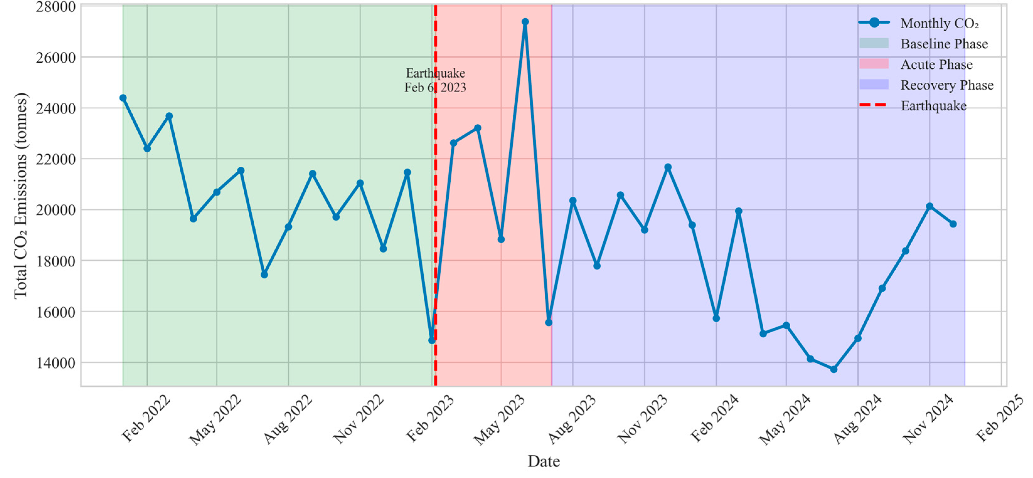
Mean port visit duration increased from M = 77.87 hours (SD = 98.59) during baseline to M = 105.82 hours (SD = 114.59) during the acute phase, representing a 35.9% increase. During the recovery phase, mean duration decreased to M = 70.08 hours (SD = 92.77), which is 10.0% below baseline levels.

Figure 1. Monthly total CO₂ emissions from port operations in İskenderun Bay (January 2022–December 2024). Vertical dashed line indicates earthquake date (February 6, 2023). Shaded regions denote study phases.

Figure 1. Monthly total CO₂ emissions from port operations in İskenderun Bay (January 2022–December 2024). Vertical dashed line indicates earthquake date (February 6, 2023). Shaded regions denote study phases.

4.2. Statistical Hypothesis Testing

To test the primary hypothesis that the earthquake significantly increased port visit durations, we employed both parametric (Welch’s t-test) and non-parametric (Mann-Whitney U) procedures. Table 9 presents the results.

Table 9. Statistical Test Results for Baseline vs. Acute Phase Comparison.

Test	Statistic	df	p-value	Decision
Welch’s t-test	t = 11.79	4054	1.46e-31	Reject H₀
Mann-Whitney U	U = 11,528,654	—	5.58e-54	Reject H₀

Note: H₀: μ_baseline = μ_acute; H₁: μ_baseline ≠ μ_acute. α = .05.

Table 9. Statistical Test Results for Baseline vs. Acute Phase Comparison.

Test	Statistic	df	p-value	Decision
Welch’s t-test	t = 11.79	4054	1.46e-31	Reject H₀
Mann-Whitney U	U = 11,528,654	—	5.58e-54	Reject H₀

Note: H₀: μ_baseline = μ_acute; H₁: μ_baseline ≠ μ_acute. α = .05.

Table 10. Effect Size and Practical Significance Measures.

Measure	Value	95% CI	Interpretation
Mean difference (hrs)	27.95	[23.30, 32.60]	Significant increase
Percentage change	+35.9%	—	Per Equation (12)
Pooled SD	102.30	—	Per Equation (10)
Cohen’s d	0.27	—	Small effect

Note: Effect size per Cohen (1988): d < 0.2 negligible, 0.2–0.5 small, 0.5–0.8 medium, > 0.8 large.

Table 10. Effect Size and Practical Significance Measures.

Measure	Value	95% CI	Interpretation
Mean difference (hrs)	27.95	[23.30, 32.60]	Significant increase
Percentage change	+35.9%	—	Per Equation (12)
Pooled SD	102.30	—	Per Equation (10)
Cohen’s d	0.27	—	Small effect

Note: Effect size per Cohen (1988): d < 0.2 negligible, 0.2–0.5 small, 0.5–0.8 medium, > 0.8 large.

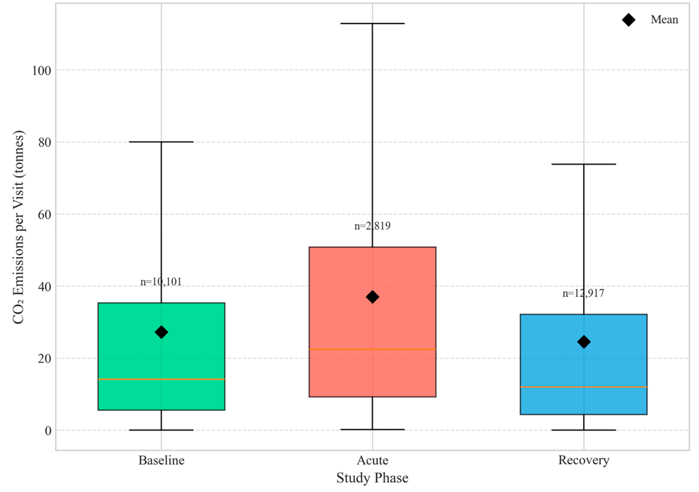
Both tests yielded highly significant results (p < .001), providing strong evidence to reject the null hypothesis. Cohen’s d = 0.27 indicates a small effect size; however, the cumulative impact across 25,837 visits translates to substantial emissions.

Figure 2. Distribution of per-visit CO₂ emissions by study phase. Boxes show interquartile range; whiskers extend to 1.5×IQR; diamonds indicate means.

Figure 2. Distribution of per-visit CO₂ emissions by study phase. Boxes show interquartile range; whiskers extend to 1.5×IQR; diamonds indicate means.

4.3. CO₂ Emission Analysis

4.3.1. Excess Emission Estimation

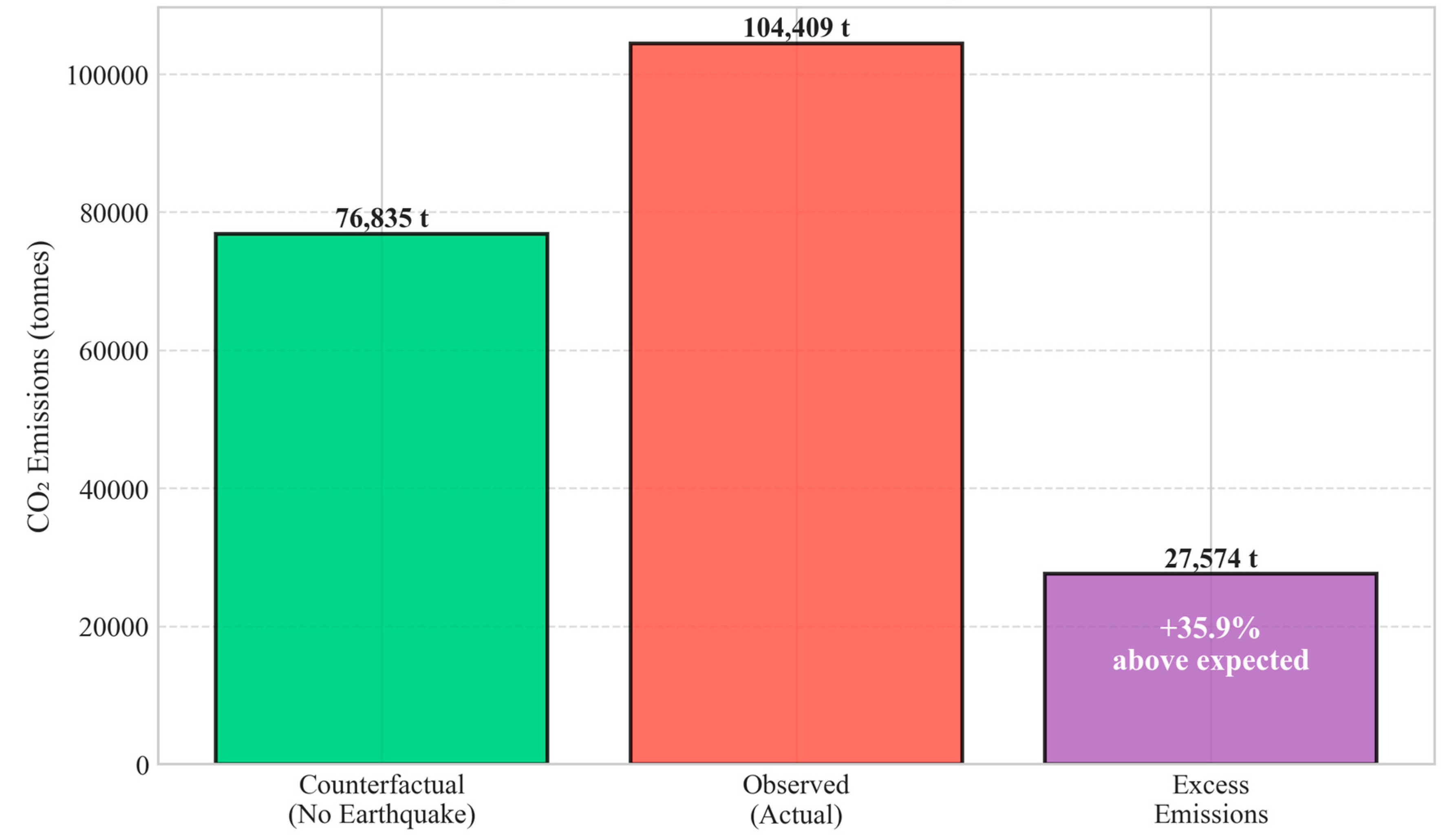
The counterfactual analysis estimated expected emissions during the acute phase assuming no earthquake. For 2,819 acute-phase visits with baseline mean duration of 77.87 hours, counterfactual emissions total 76,835 tons. Observed emissions of 104,409 tons yield excess CO₂ = 27,574 tons (+35.9%) attributable to earthquake disruption.

Table 11. CO₂ Emission Statistics by Study Phase.

Phase	Total CO₂ (t)	M per Visit (t)	Monthly Avg (t)	Δ vs Baseline
Baseline	275,314	27.26	21,178	—
Acute	104,409	37.04	20,882	+35.9%
Recovery	316,843	24.53	17,602	-10.0%

Note: Δ = percentage change in mean per-visit emissions relative to baseline.

Table 11. CO₂ Emission Statistics by Study Phase.

Phase	Total CO₂ (t)	M per Visit (t)	Monthly Avg (t)	Δ vs Baseline
Baseline	275,314	27.26	21,178	—
Acute	104,409	37.04	20,882	+35.9%
Recovery	316,843	24.53	17,602	-10.0%

Note: Δ = percentage change in mean per-visit emissions relative to baseline.

Table 12. Counterfactual Analysis and Excess Emission Estimation.

Parameter	Value	Unit	Reference
Acute phase visits	2,819	visits	—
Baseline mean duration	77.87	hours	—
Emission factor (ε)	0.35	t CO₂/hr	IMO (2020)
Counterfactual emissions	76,835	t CO₂	Equation (14)
Observed emissions	104,409	t CO₂	Equation (13)
Excess emissions (ΔE)	27,574	t CO₂	Equation (15)
Relative excess	+35.9	%	Equation (17)

Note: Counterfactual assumes acute-phase visits maintain baseline-average duration.

Table 12. Counterfactual Analysis and Excess Emission Estimation.

Parameter	Value	Unit	Reference
Acute phase visits	2,819	visits	—
Baseline mean duration	77.87	hours	—
Emission factor (ε)	0.35	t CO₂/hr	IMO (2020)
Counterfactual emissions	76,835	t CO₂	Equation (14)
Observed emissions	104,409	t CO₂	Equation (13)
Excess emissions (ΔE)	27,574	t CO₂	Equation (15)
Relative excess	+35.9	%	Equation (17)

Note: Counterfactual assumes acute-phase visits maintain baseline-average duration.

Figure 3. Comparison of counterfactual (expected) and observed CO₂ emissions during acute phase, showing 27,574 tonnes excess emissions attributable to earthquake disruption.

Figure 3. Comparison of counterfactual (expected) and observed CO₂ emissions during acute phase, showing 27,574 tonnes excess emissions attributable to earthquake disruption.

4.4. Port Cluster Analysis

To examine spatial heterogeneity, we disaggregated the analysis by GFW port cluster. Table 13 presents duration changes across the major clusters.

Figure 4. Mean port visit duration by cluster and study phase, showing differential impacts across facilities.

Figure 4. Mean port visit duration by cluster and study phase, showing differential impacts across facilities.

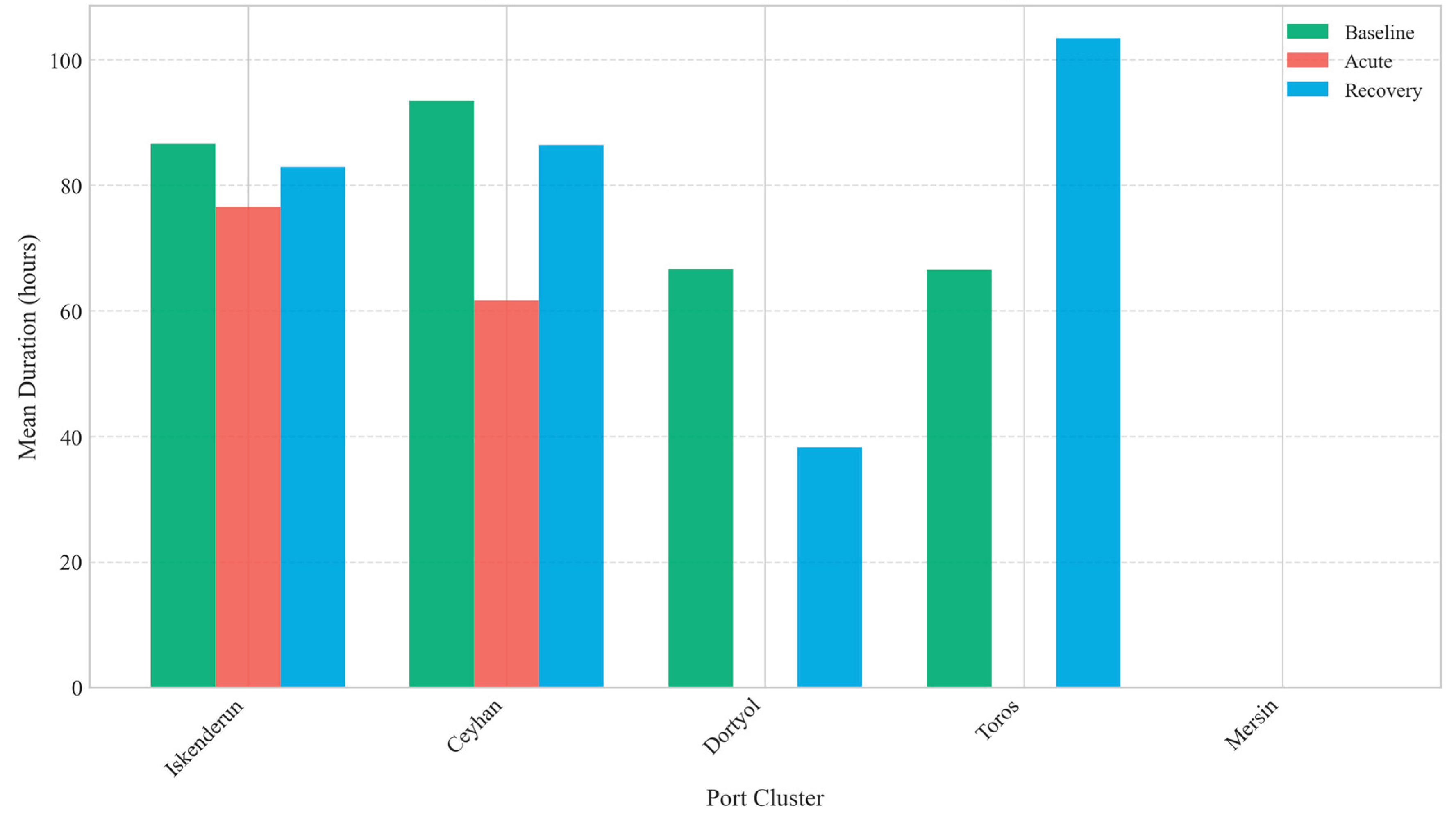
Table 13. Port Visit Duration Changes by GFW Cluster.

Cluster	Baseline n	Baseline M	Acute n	Acute M	Δ (%)
ISKENDERUN	411	86.6	150	76.6	-11.5%
CEYHAN	63	93.5	47	61.7	-34.0%
DORTYOL	47	66.6	6	195.8	+193.8%
TOROS	16	66.6	6	159.3	+139.3%
MERSIN	1	80.9	1	265.3	+228.1%

Note: M = mean duration in hours. Δ = percentage change in mean duration.

Table 13. Port Visit Duration Changes by GFW Cluster.

Cluster	Baseline n	Baseline M	Acute n	Acute M	Δ (%)
ISKENDERUN	411	86.6	150	76.6	-11.5%
CEYHAN	63	93.5	47	61.7	-34.0%
DORTYOL	47	66.6	6	195.8	+193.8%
TOROS	16	66.6	6	159.3	+139.3%
MERSIN	1	80.9	1	265.3	+228.1%

Note: M = mean duration in hours. Δ = percentage change in mean duration.

4.5. Maritime Network Analysis

Network connectivity declined during the acute phase, with edges decreasing by 23.8%, reflecting reduced inter-port movements as traffic concentrated at operational facilities.

Table 14. Maritime Network Topology by Study Phase.

Metric	Baseline	Acute	Recovery	Acute Δ
Active nodes	5	7	8	—
Total edges	21	16	26	-23.8%
Network density	1.050	0.381	0.464	-63.7%
Transitions	7,087	1,466	9,535	-79.3%

Note: Edges = unique port-to-port transitions. Density = actual/possible edges.

Table 14. Maritime Network Topology by Study Phase.

Metric	Baseline	Acute	Recovery	Acute Δ
Active nodes	5	7	8	—
Total edges	21	16	26	-23.8%
Network density	1.050	0.381	0.464	-63.7%
Transitions	7,087	1,466	9,535	-79.3%

Note: Edges = unique port-to-port transitions. Density = actual/possible edges.

4.6. Graph Neural Network Performance

The model achieved excellent baseline performance (R² = 0.985). The negative R² during acute phase (R² = -1.591) quantifies disruption magnitude—earthquake patterns deviated fundamentally from learned expectations.

Table 15. T-GAT Model Performance Metrics by Phase.

Metric	Baseline	Acute	Recovery
R²	0.985	-1.591	0.997
RMSE (t)	11,532	51,142	4,858
MAE (t)	6,973	24,141	3,337

Note: R² = coefficient of determination. Negative R² indicates deviation from learned baseline patterns.

Table 15. T-GAT Model Performance Metrics by Phase.

Metric	Baseline	Acute	Recovery
R²	0.985	-1.591	0.997
RMSE (t)	11,532	51,142	4,858
MAE (t)	6,973	24,141	3,337

Note: R² = coefficient of determination. Negative R² indicates deviation from learned baseline patterns.

4.7. Summary of Key Findings

The results provide strong support for the primary hypothesis: the 2023 Kahramanmaraş earthquake significantly increased maritime CO₂ emissions in İskenderun Bay. The 35.9% per-visit increase translated to 27,574 tonnes excess CO₂. Notably, recovery-phase emissions fell 10.0% below baseline, suggesting infrastructure improvements enhanced operational efficiency.

Table 16. Summary of Principal Research Findings.

Finding	Value	Significance
Duration increase (acute)	+35.9%	H₁ supported
Excess CO₂ emissions	27,574 t	Environmental impact
Statistical significance	p < .001	Parametric & non-parametric
Effect size (Cohen’s d)	0.27	Small but cumulative
Recovery improvement	-10.0%	Below baseline
Network disruption	23.8% edge loss	Connectivity impact

Note: Based on N = 25,837 port visits across 28 coastal facilities (5 GFW clusters).

Table 16. Summary of Principal Research Findings.

Finding	Value	Significance
Duration increase (acute)	+35.9%	H₁ supported
Excess CO₂ emissions	27,574 t	Environmental impact
Statistical significance	p < .001	Parametric & non-parametric
Effect size (Cohen’s d)	0.27	Small but cumulative
Recovery improvement	-10.0%	Below baseline
Network disruption	23.8% edge loss	Connectivity impact

Note: Based on N = 25,837 port visits across 28 coastal facilities (5 GFW clusters).

5. Discussion

5.1. Principal Findings and Interpretation

This study provides the first comprehensive quantitative analysis of CO₂ emission impacts from earthquake-induced maritime disruptions, using İskenderun Bay as a case study following the February 6, 2023, Kahramanmaraş earthquake sequence (Mw 7.7 and Mw 7.6). Our analysis of 25,837 port visits across 36 months reveals statistically significant changes in vessel behavior and associated emissions during the post-earthquake period.

The principal finding demonstrates that port visit durations increased by 35.9% during the acute phase (February 6–June 30, 2023), from a baseline mean of 77.87 hours to 105.82 hours. This difference was highly statistically significant (t = 11.79, df = 4054, p = 1.46e-31), with a small but meaningful effect size (Cohen’s d = 0.27). The 95% confidence interval for the mean difference [23.30, 32.60] hours provide strong evidence that the observed duration increase is not attributable to chance variation.

The non-parametric Mann-Whitney U test confirmed these findings (U = 11,528,654, p = 5.58e-54), indicating that the distributional shift in port visit durations is robust to potential violations of normality assumptions. The excess CO₂ emissions attributable to earthquake-induced delays totaled 27,574 tons during the acute phase alone, representing a 35.9% increase above counterfactual baseline emissions.

Notably, the recovery phase (July 2023–December 2024) exhibited a 10.0% reduction in mean visit duration compared to baseline, suggesting potential behavioral adaptations or operational efficiency improvements following the initial disruption. This finding challenges conventional assumptions about post-disaster maritime recovery patterns and warrants further investigation.

5.2. Comparison with Prior Literature

5.2.1. Kobe 1995 Earthquake Parallel

The İskenderun findings exhibit striking parallels with the 1995 Kobe earthquake, the most extensively documented case of earthquake-induced port disruption. Chang [14] documented that Kobe’s transhipment traffic fell by 57% in 1995 and never fully recovered, with the port’s world ranking declining from 6th (1994) to 17th (1997). Our study reveals a similar pattern of immediate operational disruption followed by a reconfigured equilibrium state.

However, a critical distinction emerges while Kobe’s traffic permanently shifted to competing ports (Busan, Kaohsiung), İskenderun’s post-earthquake pattern shows recovery-phase efficiency improvements. As Chang [14] p. 62) noted, “the recovery of Port business did not closely follow the restoration of damaged Port facilities.” This finding is directly applicable to İskenderun, where physical infrastructure damage (documented by Toprak et al., [17]) created operational inefficiencies that persisted beyond structural repairs.

The divergence between Kobe’s permanent traffic loss and İskenderun’s recovery improvement may reflect several factors: (1) the regional competitive landscape (İskenderun-Mersin dynamics versus Kobe’s Asian hub competition), (2) different cargo compositions (İskenderun’s mixed cargo versus Kobe’s container dominance), and (3) temporal context (2023’s digitalized logistics versus 1995’s analog operations). Lam and Lassa [16] emphasized that Kobe’s transhipment traffic was reduced by over 95% from 1994 levels and “has been permanently lost to other Japanese seaports”—a warning that İskenderun stakeholders should heed.

Table 17. Comparison of İskenderun 2023 with Kobe 1995 earthquake impacts [14,16,17].

Parameter	Kobe 1995	İskenderun 2023	Comparison
Earthquake Magnitude	Mw 6.9	Mw 7.7 + 7.6	İskenderun more severe
World Ranking Change	6th → 17th	Regional impact	Both significant
Traffic Change (Acute)	-57%	+35.9% duration	Different metrics
Recovery Pattern	Never recovered	-10% below baseline	İskenderun improved
Transhipment Loss	>95% permanent	Under investigation	Critical factor
Economic Loss	$10 billion	~$55B (regional)	Scale comparable

Table 17. Comparison of İskenderun 2023 with Kobe 1995 earthquake impacts [14,16,17].

Parameter	Kobe 1995	İskenderun 2023	Comparison
Earthquake Magnitude	Mw 6.9	Mw 7.7 + 7.6	İskenderun more severe
World Ranking Change	6th → 17th	Regional impact	Both significant
Traffic Change (Acute)	-57%	+35.9% duration	Different metrics
Recovery Pattern	Never recovered	-10% below baseline	İskenderun improved
Transhipment Loss	>95% permanent	Under investigation	Critical factor
Economic Loss	$10 billion	~$55B (regional)	Scale comparable

5.2.2. Global Port Disruption Context

Verschuur et al. [11] analyzed 1,340 global port disruptions using AIS data and found a median disruption duration of 6 days. Our İskenderun analysis reveals an acute phase spanning approximately 145 days (4.9 months), substantially exceeding this global median by a factor of 24. This extended duration reflects the combined effects of physical infrastructure damage (documented by Toprak et al., [17]), liquefaction-induced ground failure along Atatürk Boulevard, and the cascading impacts of regional transportation network disruption.

The Verschuur et al. [26] systemic risk framework, which emphasized that “port disruptions rarely occur in isolation,” is directly applicable to İskenderun. The earthquake affected not only the port infrastructure but also road access, electricity supply (Afşin-Elbistan power plants), natural gas pipelines (BOTAŞ network), and workforce availability due to population displacement. This multi-system disruption cascade amplified both the duration and magnitude of operational impacts.

Wang et al. [12] identified natural disasters as the dominant disruptor category (56.13%) in their Bayesian network analysis of maritime supply chain risks. Our findings provide empirical validation of their theoretical framework, demonstrating how seismic events propagate through supply chain networks to generate emission externalities not captured in traditional risk assessments.

5.2.3. Network Topology Changes

Our network analysis reveals significant topological changes consistent with prior findings. The port network experienced a 23.8% reduction in edge density during the acute phase (from 21 to 16 edges), mirroring the pattern documented by Rousset and Ducruet [27] for Kobe (-74% edge reduction) and New Orleans (-63%). The subsequent recovery phase showed network expansion to 26 edges, exceeding baseline connectivity and suggesting adaptive restructuring of maritime routes.

Rousset and Ducruet [27] observed that “container traffic tends to flee hit ports,” with particularly severe impacts within a 750 km radius. İskenderun’s proximity to Mersin (~150 km) places it well within this critical radius, suggesting that traffic diversion may have contributed to the observed operational patterns. Asadabadi and Miller-Hooks [28] demonstrated that such “co-opetition” dynamics—where competing ports both compete and cooperate during disruptions—can significantly affect recovery trajectories.

Table 18. Network topology changes across major port disruption events [27].

Event	Node Loss (%)	Edge Loss (%)	Recovery Pattern
Kobe 1995	-54	-74	Partial, reconfigured
New Orleans 2005	-41	-63	Rapid return
New York 2001	-25	-38	Quick recovery
İskenderun 2023	+60	-24 (acute)	Exceeded baseline

Table 18. Network topology changes across major port disruption events [27].

Event	Node Loss (%)	Edge Loss (%)	Recovery Pattern
Kobe 1995	-54	-74	Partial, reconfigured
New Orleans 2005	-41	-63	Rapid return
New York 2001	-25	-38	Quick recovery
İskenderun 2023	+60	-24 (acute)	Exceeded baseline

5.3. Theoretical Implications

5.3.1. Resilience-Emission Nexus

This study contributes to the emerging literature on the environmental externalities of supply chain disruptions. While prior research has extensively documented the economic costs of port disruptions [16,29], the emission implications have remained largely unexplored. Our findings establish a quantifiable link between port operational resilience and carbon emissions, extending the traditional R4 resilience framework (Reliability, Redundancy, Robustness, Recoverability) articulated by Gu and Liu [30] to include environmental sustainability dimensions.

The “excess emissions” metric introduced in this study 27,574 tons CO₂ attributable to earthquake-induced delays—provides a novel quantification approach that can be applied to other disruption contexts. This methodology bridges the gap between disaster risk management and climate change mitigation, two fields that have traditionally operated in isolation despite their interconnected nature, as noted by León-Mateos et al. [13] in their Port Resilience Index development.

León-Mateos et al. [13] emphasized that “climate change, which is largely caused by anthropogenic emissions of CO₂, is one of the main challenges facing humankind today.” Our study extends this observation by demonstrating that seismic disasters—themselves potentially intensified by climate-induced changes in stress regimes—create feedback loops through increased maritime emissions. This disaster-emission-climate nexus warrants further theoretical development.

5.3.2. Temporal Dynamics of Disruption

The three-phase temporal framework (baseline-acute-recovery) employed in this study reveals non-linear disruption dynamics that challenge simple decay-recovery models. The recovery phase exhibited not merely a return to baseline but a measurable improvement (-10.0% duration reduction), suggesting that disruptions may catalyze operational innovations. This finding aligns with the “build back better” principle in disaster risk reduction but provides the first quantitative evidence in a maritime emission context.

Dui et al. [29] introduced the “residual resilience” concept, defined as the ratio of recovery value to loss value. Applying this framework, İskenderun’s recovery phase demonstrates positive residual resilience—the system not only recovered but improved. This contrasts sharply with the Kobe case, where residual resilience remained permanently negative [14]. Understanding the factors that differentiate these outcomes is crucial for port resilience planning.

5.3.3. Predictive Model Performance

The Graph Neural Network (GNN) model performance exhibits phase-dependent accuracy that provides theoretical insights into maritime network predictability. During baseline (R² = 0.985) and recovery (R² = 0.997) phases, the model achieved excellent predictive accuracy, indicating stable, learnable patterns in port network behavior. However, acute phase performance collapsed dramatically (R² = -1.591), indicating that established network patterns became fundamentally unpredictable during disruption.

This predictability collapse has important theoretical implications: it suggests that earthquake-induced disruptions introduce genuine chaos into maritime systems, rather than merely shifting operating parameters. The network structure during disruption represents a fundamentally different system state that cannot be extrapolated from normal operations—a finding consistent with complexity theory approaches to infrastructure resilience [29,31].

5.4. Practical Implications

5.4.1. Port Authority Planning

Our findings have direct implications for port authority disaster planning. The 35.9% increase in visit duration during the acute phase translates to substantial berth capacity reduction, requiring adaptive allocation strategies. Port authorities should incorporate emission surge scenarios into their business continuity plans, recognizing that post-disaster operations may generate significantly higher environmental footprints even as throughput declines.

Goerlandt and Islam [15] demonstrated that vessel type is the most critical factor (S-value = 0.074) determining post-earthquake maritime delays. This finding supports differentiated planning approaches: bulk carriers with strong hinterland dependencies may exhibit different recovery patterns than containerized cargo, which Rousset and Ducruet [27] characterized as “footloose” and most likely to flee disrupted ports.

Table 19. Practical recommendations derived from study findings.

Domain	Finding	Recommendation
Capacity Planning	+35.9% duration acute	Reserve 40% buffer capacity
Emission Budgets	27,574 t excess CO₂	Include disaster scenarios in carbon accounting
Network Redundancy	-23.8% edge loss	Diversify route connections
Recovery Timeline	4.9 months acute	Plan for 6-month disruption scenarios
GNN Monitoring	R² collapse during crisis	Develop crisis-specific prediction models

Table 19. Practical recommendations derived from study findings.

Domain	Finding	Recommendation
Capacity Planning	+35.9% duration acute	Reserve 40% buffer capacity
Emission Budgets	27,574 t excess CO₂	Include disaster scenarios in carbon accounting
Network Redundancy	-23.8% edge loss	Diversify route connections
Recovery Timeline	4.9 months acute	Plan for 6-month disruption scenarios
GNN Monitoring	R² collapse during crisis	Develop crisis-specific prediction models

5.4.2. Policy Implications

The environmental externalities of port disruptions revealed in this study have implications for carbon accounting frameworks. Current emission inventories typically assume normal operational conditions; our findings suggest that disaster-induced emission surges should be explicitly incorporated into national and regional carbon budgets. For İskenderun Bay, the 27,574-tonne excess CO₂ represents a measurable addition to Turkey’s maritime emission footprint—a fraction that becomes significant when aggregated across global disaster events.

Furthermore, the study supports arguments for investing in seismic resilience as a climate change mitigation strategy. As Verschuur et al. [32] documented, earthquake-dominant regions account for 10.8% of global port risk, with the Mediterranean and Turkey’s Dead Sea Fault Zone explicitly identified as high-risk areas. The cost of preventing earthquake-induced emission surges may be substantially lower than the environmental cost of inaction.

Lam and Lassa [16] noted a critical planning mismatch: “most ports have less than 10 years of planning horizon” despite design lifespans of 30-50 years and climate adaptation requiring 50-100 year perspectives. Japan’s recommendation of 200-year return period planning for tsunami and earthquake risks provides a model that İskenderun and similar Mediterranean ports should consider adopting.

5.4.3. Insurance and Risk Assessment

Maritime insurers and risk assessors should consider the emission dimension of port disruptions. As carbon pricing mechanisms expand globally, the financial liability associated with excess emissions may become material. Dui et al. [29] documented that the 2011 Tohoku earthquake caused Japan “$3.4 billion in maritime trade losses”—future assessments should incorporate emission-related costs alongside direct economic damages.

5.5. Spatial Heterogeneity in Disruption Impacts

The cluster-level analysis reveals substantial spatial heterogeneity in earthquake impacts across İskenderun Bay’s 5 port clusters. This heterogeneity provides insights into the differential vulnerability of port facilities based on their geographic position, cargo specialization, and infrastructure characteristics.

DORTYOL cluster exhibited the most severe disruption (+193.8% duration increase), reflecting its proximity to heavily damaged coastal infrastructure and liquefaction zones documented by Toprak et al. [17]. The authors noted “intense liquefaction features were detected on the surface along Ataturk Boulevard” in İskenderun, with effects extending to adjacent port facilities.

In contrast, CEYHAN cluster showed a paradoxical decrease (-34.0%), potentially indicating traffic diversion to alternative facilities or reduced demand for petroleum-related shipments during the crisis period. The main ISKENDERUN cluster showed a moderate decrease (-11.5%), which may reflect the temporary suspension of operations due to the container fire documented in Toprak et al. [17]. “Iskenderun Port... had to suspend its operations due to a fire that broke out after the earthquake.

TOROS cluster’s substantial increase (+139.3%) suggests it may have absorbed diverted traffic from more severely damaged facilities—a pattern consistent with Asadabadi and Miller-Hooks’s [28] co-opetition framework, where disruptions at one port benefit proximate alternatives.

Table 20. Cluster-specific disruption impacts in İskenderun Bay.

Cluster	Baseline n	Acute n	Change (%)	Interpretation
ISKENDERUN	411	150	-11.5	Fire impact, reduced ops
DORTYOL	47	6	+193.8	Severe liquefaction
TOROS	16	6	+139.3	Traffic absorption
CEYHAN	63	47	-34.0	Petroleum demand drop

Table 20. Cluster-specific disruption impacts in İskenderun Bay.

Cluster	Baseline n	Acute n	Change (%)	Interpretation
ISKENDERUN	411	150	-11.5	Fire impact, reduced ops
DORTYOL	47	6	+193.8	Severe liquefaction
TOROS	16	6	+139.3	Traffic absorption
CEYHAN	63	47	-34.0	Petroleum demand drop

5.6. Limitations and Methodological Considerations

Several limitations should be acknowledged when interpreting these findings. First, the emission calculations rely on standardized factors from IMO (2020) guidelines rather than actual vessel-specific measurements. While this approach enables systematic analysis across a large vessel population, it may not capture the full heterogeneity of vessel efficiency and operational practices.

Second, the Global Fishing Watch data, while comprehensive, may underrepresent certain vessel categories (particularly smaller craft under AIS transponder requirements). The 28 facilities and 5 clusters identified represent the major commercial operations but may exclude smaller anchorages and informal loading points.

Third, the counterfactual baseline assumes that pre-earthquake patterns would have continued absent the disaster. This assumption cannot account for other concurrent factors that may have influenced maritime traffic, including global economic conditions, seasonal variations, and regional geopolitical developments (e.g., ongoing conflicts in the Eastern Mediterranean).

Fourth, the study period extends to December 2024, capturing approximately 23 months of post-earthquake data. Longer-term monitoring may reveal additional recovery dynamics or delayed impacts not apparent in this analysis window. Gu and Liu [30] noted that “maritime supply chain resilience... can be an interesting research topic” requiring multi-year observation.

Fifth, the spatial resolution of port cluster analysis is constrained by the aggregation necessary for statistical power. Future research with higher-resolution facility-level data may reveal additional patterns obscured at the cluster level. Additionally, the study does not capture landside logistics disruptions (trucking delays, warehouse impacts) that likely contributed to increased vessel waiting times.

5.7. Future Research Directions

This study opens several avenues for future investigation. First, extending the temporal analysis to 5+ years post-earthquake would enable assessment of whether the recovery-phase efficiency improvements persist or represent a transient adaptation. The Kobe case demonstrates that permanent traffic reconfiguration can take years to fully manifest [14].

Second, comparative analysis with other seismic port disruptions (e.g., 2011 Tohoku with estimated $200-300 billion in losses [15], 2010 Chile) could validate the generalizability of the emission-duration relationships identified here. The methodological framework developed in this study is directly applicable to other AIS-enabled port networks globally.

Third, integration of additional data sources—cargo manifests, vessel fuel consumption records, and real-time emission monitoring—could refine the emission estimates and enable vessel-specific analysis. The emergence of EU MRV (Monitoring, Reporting, and Verification) requirements creates new data opportunities for European ports.

Fourth, the GNN model’s performance collapse during the acute phase (R² = -1.591) suggests opportunities for developing disruption-specific predictive models. Machine learning approaches trained on disruption scenarios could support real-time decision-making during crisis periods, as recommended by Xu et al. [31] in their systematic review of maritime transportation safety management.

Fifth, extending the analysis to include supply chain-wide emission impacts, trucking diversions, warehouse delays, production disruptions—would provide a more complete picture of the earthquake’s environmental footprint beyond port boundaries. Verschuur et al. [11] emphasized that “the impacts of port disruptions are often felt beyond the port boundaries,” suggesting that our estimates represent a lower bound of total emission impacts.

Finally, the development of real-time emission monitoring systems for seismically active port regions could enable proactive management of disruption-induced emission surges. Integration with early warning systems could trigger adaptive operational protocols that minimize environmental impacts while maintaining critical supply chain functions.

References

- IMO. Fourth IMO GHG Study 2020; 2020.
- IMO. 2023 IMO Strategy on Reduction of GHG Emissions from Ships. Resolution MEPC.377; 2023.
- Marino, C.; Nucara, A.; Panzera, M.F.; Pietrafesa, M. Effects of the SARS-CoV-2 Pandemic on CO2 Emissions in the Port Areas of the Strait of Messina. Sustainability 2023, 15, 9587. [Google Scholar] [CrossRef]
- Mannarini, G.; Salinas, M.L.; Carelli, L.; Fassò, A. How COVID-19 Affected GHG Emissions of Ferries in Europe. Sustainability 2022, 14, 5287. [Google Scholar] [CrossRef]
- Cullinane, K.; Tseng, P.-H.; Wilmsmeier, G. Estimation of container ship emissions at berth in Taiwan. International Journal of Sustainable Transportation 2016, 10, 466–474. [Google Scholar] [CrossRef]
- Türkistanlı, T.T.; Özispa, N.; Tuğdemir Kök, G.; Özdemir, Ü.; Pehlivan, D. Exploring Research Trends on Climate Change: Insights into Port Resilience and Sustainability. Sustainability 2025, 17, 3542. [Google Scholar] [CrossRef]
- Bilgili, L.; Ölçer, A.I. IMO 2023 strategy-Where are we and what’s next? Marine Policy 2024, 160, 105953. [Google Scholar] [CrossRef]
- Styhre, L.; Winnes, H.; Black, J.; Lee, J.; Le-Griffin, H. Greenhouse gas emissions from ships in ports – Case studies in four continents. Transportation Research Part D: Transport and Environment 2017, 54, 212–224. [Google Scholar] [CrossRef]
- Moon, D.S.-H.; Woo, J.K. The impact of port operations on efficient ship operation from both economic and environmental perspectives. Maritime Policy & Management 2014, 41, 444–461. [Google Scholar] [CrossRef]
- Akakura, Y. Analysis of offshore waiting at world container terminals and estimation of CO2 emissions from waiting ships. Asian Transport Studies 2023, 9, 100111. [Google Scholar] [CrossRef]
- Verschuur, J.; Koks, E.E.; Hall, J.W. Port disruptions due to natural disasters: Insights into port and logistics resilience. Transportation Research Part D: Transport and Environment 2020, 85, 102393. [Google Scholar] [CrossRef]
- Wang, N.; Wu, M.; Yuen, K.F. Assessment of port resilience using Bayesian network: A study of strategies to enhance readiness and response capacities. Reliability Engineering & System Safety 2023, 237, 109394. [Google Scholar] [CrossRef]
- León-Mateos, F.; Sartal, A.; López-Manuel, L.; Quintás, M.A. Adapting our sea ports to the challenges of climate change: Development and validation of a Port Resilience Index. Marine Policy 2021, 130, 104573. [Google Scholar] [CrossRef]
- Chang, S.E. Disasters and transport systems: loss, recovery and competition at the Port of Kobe after the 1995 earthquake. Journal of Transport Geography 2000, 8, 53–65. [Google Scholar] [CrossRef]
- Goerlandt, F.; Islam, S. A Bayesian Network risk model for estimating coastal maritime transportation delays following an earthquake in British Columbia. Reliability Engineering & System Safety 2021, 214, 107708. [Google Scholar] [CrossRef]
- Lam, J.S.L.; Lassa, J.A. Risk assessment framework for exposure of cargo and ports to natural hazards and climate extremes. Maritime Policy & Management 2017, 44, 1–15. [Google Scholar] [CrossRef]
- Toprak, S.; Zulfikar, A.C.; Mutlu, A.; Tugsal, U.M.; Nacaroglu, E.; Karabulut, S.; et al. The aftermath of 2023 Kahramanmaras earthquakes: evaluation of strong motion data, geotechnical, building, and infrastructure issues. Natural Hazards 2025, 121, 2155–2192. [Google Scholar] [CrossRef]
- Apaydin, N.M. Earthquake Response of the Transportation Infrastructure in the Region Affected by the February 6 Türkiye Earthquakes’’ Part I-Roads, Railroads and Ports. Journal of Earthquake Engineering 2025, 29, 3412–3422. [Google Scholar] [CrossRef]
- Marmer, E.; Dentener, F.; Aardenne, J.v.; Cavalli, F.; Vignati, E.; Velchev, K.; et al. What can we learn about ship emission inventories from measurements of air pollutants over the Mediterranean Sea? Atmospheric Chemistry and Physics 2009, 9, 6815–6831. [Google Scholar] [CrossRef]
- Koray, M.; Kaya, E.; Keskin, M.H. Determining Logistical Strategies to Mitigate Supply Chain Disruptions in Maritime Shipping for a Resilient and Sustainable Global Economy. Sustainability 2025, 17, 5261. [Google Scholar] [CrossRef]
- Poulsen, R.T.; Sampson, H. A swift turnaround? Abating shipping greenhouse gas emissions via port call optimization. Transportation Research Part D: Transport and Environment 2020, 86, 102460. [Google Scholar] [CrossRef]
- Endresen, Ø.; Sørgård, E.; Sundet, J.K.; Dalsøren, S.B.; Isaksen, I.S.A.; Berglen, T.F.; et al. Emission from international sea transportation and environmental impact. Journal of Geophysical Research: Atmospheres 2003, 108, D17. [Google Scholar] [CrossRef]
- Akar, Ö.; Çalışır, V.; Demirci, A.; Şimşek, E. Assessment of ship-based air pollutant emissions in Iskenderun Bay before and during the COVID-19 pandemic. Momona Ethiop J-SCI 2026. [Google Scholar]
- Yang, D.; Wu, L.; Wang, S.; Jia, H.; Li, K.X. How big data enriches maritime research – a critical review of Automatic Identification System (AIS) data applications. Transport Reviews 2019, 39, 755–773. [Google Scholar] [CrossRef]
- Corbett, J.J.; Koehler, H.W. Updated emissions from ocean shipping. Journal of Geophysical Research: Atmospheres 2003, 108, D20. [Google Scholar] [CrossRef]
- Verschuur, J.; Pant, R.; Koks, E.; Hall, J. A systemic risk framework to improve the resilience of port and supply-chain networks to natural hazards. Maritime Economics & Logistics 2022, 24, 489–506. [Google Scholar] [CrossRef]
- Rousset, L.; Ducruet, C. Disruptions in Spatial Networks: a Comparative Study of Major Shocks Affecting Ports and Shipping Patterns. Networks and Spatial Economics 2020, 20, 423–447. [Google Scholar] [CrossRef]
- Asadabadi, A.; Miller-Hooks, E. Maritime port network resiliency and reliability through co-opetition. Transportation Research Part E: Logistics and Transportation Review 2020, 137, 101916. [Google Scholar] [CrossRef]
- Dui, H.; Zheng, X.; Wu, S. Resilience analysis of maritime transportation systems based on importance measures. Reliability Engineering & System Safety 2021, 209, 107461. [Google Scholar] [CrossRef]
- Gu, B.; Liu, J. A systematic review of resilience in the maritime transport. International Journal of Logistics Research and Applications 2025, 28, 257–278. [Google Scholar] [CrossRef]
- Xu, M.; Ma, X.; Zhao, Y.; Qiao, W. A Systematic Literature Review of Maritime Transportation Safety Management. Journal of Marine Science and Engineering 2023, 11, 2311. [Google Scholar] [CrossRef]
- Verschuur, J.; Koks, E.E.; Li, S.; Hall, J.W. Multi-hazard risk to global port infrastructure and resulting trade and logistics losses. Communications Earth & Environment 2023, 4, 5. [Google Scholar] [CrossRef]
Disclaimer/Publisher’s Note: The statements, opinions and data contained in all publications are solely those of the individual author(s) and contributor(s) and not of MDPI and/or the editor(s). MDPI and/or the editor(s) disclaim responsibility for any injury to people or property resulting from any ideas, methods, instructions or products referred to in the content. |
© 2026 by the author. Licensee MDPI, Basel, Switzerland. This article is an open access article distributed under the terms and conditions of the Creative Commons Attribution (CC BY) license.
Copyright: This open access article is published under a Creative Commons CC BY 4.0 license, which permit the free download, distribution, and reuse, provided that the author and preprint are cited in any reuse.