
Submitted:
12 January 2026
Posted:
14 January 2026
You are already at the latest version
Abstract
New general-relativistic formulations to model an elementary charge are presented, based on an electromagnetic theory of gravity, where the gravity is equivalently expressed as a gradient function of an effective permittivity distribution of the empty space. The metric tensor elements of general relativity are directly related to the effective permittivity function of the empty space, using which the energy density associated with the electric field surrounding the charge is properly defined. The empty space, represented by the equivalent permittivity function, would be fundamentally non-linear, in which case the definition of energy density, as conventionally applied for a linear medium, needs to be corrected. Further, the definition of energy density itself is modified allowing both positive and negative values, such that the total energy remains unchanged while the local values are much stronger, resulting in much stronger local gravitational effects. Solutions for the metric-tensor elements and the resulting energy/mass of the charge particle are studied, based on the Einstein-Maxwell equations with the different new formulations of the energy density and of the associated full stress-energy tensor. The solutions are verified with Schwarzschild and Reissner-Nordstrom metrics, as well as for calculation of light deflection by a massive body, as validation of the general new formulations for the specific reference cases of conventional modeling. Stable solutions for energy/mass are successfully derived for a spherically symmetric, surface distribution of an elementary charge, with specific modified definitions of energy density. A stable solution of the charge with the lowest possible energy/mass is associated with a ''static'' electron without spin. Significance of the new results and formulations, specifically established for the electron, are recognized in relation to the fine-structure constant of quantum electrodynamics, and towards further application of the theory to model other elementary particles and general electrodynamic problems.
Keywords:
elementary particle
; electromagnetic theory of gravity
; general relativity
1. Introduction
Einstein’s theory of general relativity [1,2], in the form of the Einstein field equations that govern the geometry of curved space-time, superseded the existing Newton’s theory of gravitation [3,4]. It successfully formulated the gravitational force as a fundamental manifestation of the curved structure of space-time, established in the presence of any mass/energy distribution. The theory of general relativity became highly successful to model and predict astrophysical effects, such as precession of Mercury’s orbital motion [5], and deflection of starlight due to solar gravitation [6]. Subsequently, Einstein sought to combine Maxwell’s electromagnetic theory with his new theory of gravity, so that the success of the general-relativistic formulations to astrophysical problems could possibly be extended to self-consistently model elementary charge particles, such as an electron or a proton. To this end, the general-relativistic formulations maybe combined with Maxwell’s equations, in the form of the Einstein-Maxwell equations [7]. The Reissner-Nordstrom metric [8,9] provides a solution to the Einstein-Maxwell equations, for a massive charge particle with a given mass and charge. However, the Reissner-Nordstrom metric does not lead to a self-consistent result for an elementary charge particle (electron). In fact, no self-consistent solution could be successfully established for an elementary particle, based on any such conventional formulation of the Einstein-Maxwell equations. Accordingly, the measured mass of no known elementary charge particle has been successfully derived from any such conventional theory.
An electromagnetic theory of gravity was proposed in [10], where the gravitational field could in principle be modeled in terms of an equivalent permittivity distribution of the empty space. This concept was not successfully pursued as an independent theory, because it could not compete with general relativity in terms of any new predictive or theoretical value. However, the basic concept is still physically valid, and maybe advanced in complement with the general relativity framework. Any concern in the proposed electromagnetic model of [10], in regard to possible inconsistency with observed deflection of starlight in Sun’s gravity, could be resolved. This would be possible through a hybrid interpretation by combining the definitive local deflection effect due to the non-uniform permittivity, which would as well be observed by an external global observer, with an additional contribution to transform the local effect to the global observer. Now, such an equivalent non-uniform permittivity distribution may need to be used, in order to properly define the energy density associated with the electromagnetic field surrounding a charge. Accordingly, the conventional expressions of the energy density, and the related stress-energy tensor elements, appearing in the Einstein-Maxwell equations, that are valid only in an ideal free-space medium, need to be properly corrected in terms of the new equivalent permittivity distribution. The equivalent permittivity needs to be modeled as a non linear medium, because the permittivity representing gravity would be dependent on the energy density, or equivalently on the strength of the electric field in the medium or the magnitude of the associated source charge. Further, it may also be recognized that a definition of the energy density is theoretically non-unique, as noted in [11]. Accordingly, the energy density maybe modified by adding a suitable extra term that contributes significantly strong positive and negative values at different locations, such that the total energy due to the additional term is zero. The modified energy-density would be theoretically equivalent to the original energy density, both cases resulting in the same total energy, but with significantly different local values resulting in significantly different local gravitational effects.
In this paper, we present new general-relativistic formulations in relation to an electromagnetic theory of gravity. Metric solutions for the Einstein-Maxwell equations, under different corrected or modified definitions of the stress-energy tensors are studied, with the objective of finding a self-consistent solution for a static elementary charge, such that the mass associated with a stable structure of the charge is entirely due to the energy density of the charge’s own electromagnetic field. The solutions are verified with the Schwarzschild [12,13] and the Reissner-Nordstrom [8,9] metrics, as well as for calculation of light deflection by a massive body, as validation of the general new solutions for specific reference cases of conventional modeling. Stable solutions for energy/mass are successfully derived for a spherically symmetric, surface distribution of an elementary charge, using specific modified definitions of energy density. As a simple first-order approximation, the energy density is modified with an additional term expressed as the divergence of a radial vector field proportional to the original energy density, with a suitable constant of proportionality . Assuming that the stable solution with the lowest mass/energy represents a “static” electron without any spin, the value of the new physical constant is estimated. More fundamentally, the constant , the resulting lowest stable mass of a static elementary charged particle, and the classical radius of the charge associated with the mass, are related to each other by a dimensionless constant, independent of any specific value of the charge or mass of the particle. Accordingly, by having suitable different values of the constant valid at different (smaller) radial distances from the center of the charge, the new general-relativistic formulations could in principle be extended to model other stable structures of the elementary charge, such as the proton, associated with a different (larger) mass.
The dimensionless constant derived from the above first-order model is recognized to be closely (numerologically) related to the fine-structure constant of quantum electrodynamics. The first-order approximation for the modified energy density is then substituted by a more accurate function, representing suitable second-order dependence on the original energy density, with a suitable normalized coefficient . It is shown that, the special dimensionless constant introduced above, re-derived with the second-order dependence, is precisely related to the fine-structure constant, with a suitable value of the parameter . It is a significant success, precisely tracing the origin of the fine structure constant through the proposed theory. The small difference between the dimensionless constant derived from the first- and second-order models, may perhaps provide another useful physical parameter, closely related to the deviation of electron’s measured g-factor from its first-order estimation using the fine-structure constant [14].
The presentation is partitioned into different sections as follows. The basic principles and theoretical background, based on which the rest of the analyses are advanced, are first introduced in Section 2, Section 3. The theoretical elements of an electromagnetic theory of gravity [10] are introduced in the Section 2, which is followed by key formulations of Einstein’s field theory in the Section 3, specifically established in relation to the equivalent electromagnetic model. A reference solution to the key formulations, applied in the region external to a spherical massive body, and the angular deflection of light around the body, are respectively verified with the associated Schwarzschild metric and the predicted deflection from a conventional general relativity model, in sub-Section 3.1, Section 3.2. Analysis and solutions for an elementary charge particle, with a linear modeling of the surrounding permittivity distribution, are presented in Section 4, with a specific solution that assumes an ideal free-space medium, verified with the Reissner-Nordstrom metric in sub-Section 4.1. Analysis with a more rigorous non-linear modeling of the permittivity medium, with solutions derived based on an iterative numerical method, is presented in Section 5.
Analyses and solutions based on modified energy density are presented in Section 6. These include analytical solutions for the permittivity distribution, the metric elements, and the particle’s energy/mass for a first-order modeling in sub-Section 6.1, Section 6.2, as well as numerically derived solutions based on a finite-difference/element technique for a more rigorous second-order modeling in sub-Section 6.3. The particular analysis in the sub-Section 6.1 is based on a modeling of the modified energy density using a trace-free stress-energy tensor, whereas that in the sub-Section 6.2 using an ideal fluid model of the stress-energy tensor. A reference solution for the particular analysis in the sub-Section 6.2, established internal to a uniform spherical body, is verified with the associated Schwarzschild metric in sub-Section 6.2.1. General discussions and specific conclusions are presented in the last Section 7.
2. Electromagnetic Theory of Gravity: The Basic Principles
An electromagnetic theory of gravity proposes that a gravitational field , defined as the gravitational force per unit mass , can be modeled in terms of an equivalent permittivity distribution of the empty space, at a general location [10,15,16]. This is in contrast to conventional treatment of the empty space as an ideal medium with a uniform permittivity . The proposed theory is based on a fundamental recognition that the mass , or the equivalent energy = , of a gravitating body is inversely proportional to the local permittivity , or directly proportional to the local inverse-permittivity = = . This dependence is consistent with the energy of a spherical surface charge of radius , placed at a location with permittivity . The and are the relative and inverse-relative permittivity distributions, respectively. And, the mass of the body is its intrinsic mass when placed far from any source of gravity, where the empty space is characterized as an ideal free-space with permittivity = = , or inverse-permittivity = = . Accordingly, the gravitational field maybe expressed as a gradient function of the inverse-relative permittivity distribution .
Like the permittivity distribution , the permeability of the empty space is also required to be a non-uniform distribution, in contrast to the conventional uniform value . The relative permeability is required to be equal to the relative permittivity , so that any magnetic energy associated with a mass varies in the same proportion as the electric, and therefore the total, energy as we formulated above. Accordingly, the speed of light = is non-uniform, inversely proportional to or directly proportional to the inverse-relative permittivity . is the speed of light in an ideal empty space (free-space), with .
In the equation (1), the gravitational force , and the associated gravitational field defined as the force per unit intrinsic mass (invariant with location ), are required to exhibit the standard dependence with radial distance r, in the external region of a spherical body, as observed in a global frame of reference. Accordingly, in consistency with the Newtonian gravity, the negative-divergence of the field in (1) would be proportional to the mass density = , with proportionality constant , for a general mass distribution or its equivalent energy distribution .
With proper definition for an inertial mass of a given body in a gravitational field, and its equation of motion enforced in proper space-time coordinates, the associated force field in (1,2) is expected to be consistent with general relativity. This would be validated in the following studies, verified with key reference solutions.
3. Basic General Relativity Formulation of a Spherically Symmetric Body, in Relation to the Effective Permittivity Function
The basic formulations of general relativity for a spherically symmetric structure, which maybe a charged or neutral body, consists of the Einstein field equations in terms of the Einstein tensor , the Ricci curvature tensor , and stress-energy tensor ; geodesic equation of motion in terms of the Christoffel symbols ; and metric equation in terms of metric elements [17,18].
The radial gravitational force for a spherically symmetric structure, as defined in (1), is to be properly enforced in a local frame for dynamical modeling. The local medium is associated with a non-uniform light speed , which is different from a uniform free-space medium with assumed in a Newtonian mechanics, or in the global frame of Einstein’s general relativity. Accordingly, for a stationary gravitating body in the local frame, the force F would not be equal to the body’s free-space mass times the acceleration , as would be the case using conventional Newton’s law seen in the global coordinates , but be equal to times the acceleration , where the "primed" variables are the respective transformed parameters defined in the local ("primed") coordinates. Accordingly, the gravitational force and the associated gravitational field , defined in (1,2) as per the electromagnetic theory of gravity, may now be expressed in term of its complementary metric parameters of the general relativity formulation in (5). The new mass introduced in the local coordinates is equivalent to defined in (1), which is equal to . Accordingly, the maybe defined in the general relativity framework as the free-space mass times , where the metric parameter from (5) represents the ratio of the local and global light speeds.
The above relationship (6) is established for the specific geodesic equation (4) of radial acceleration of a stationary (slow moving) body, in a spherically symmetric gravitational field, that maybe similarly extended to any general geodesic motion. The validity of (6) would be evident from the following studies, verified with key reference solutions.
The Ricci tensor elements and the Christoffel symbols used in the general relativity formulation of (3) can be shown to be expressed in the following forms for a spherically symmetric body [12,17,19].
A prime (′) notation is used in the above equations (8-11) as an alternate representation for a radial derivative (), and the notation in (7) represents a derivative with respect to the kth variable. The basic relations (7-11) would be routinely used in the following studies.
3.1. Reference Solution External to a Spherically Symmetric Body
We will solve the metric elements of (5) in the region external to a spherically symmetric body of mass M, using the new complementary frameworks established in the above Section 2, Section 3. In the external region, the stress-energy tensor and consequently the the Ricci tensor of (3) is zero. Under this condition, the relationship (10) between and is used to relate the metric elements and .
The expression of derived from the -dependent gravitational field of the spherical body, based on (2), maybe used in (6) together with the above relationship (12) between the metric elements and . This would lead to the following derivation of the metric elements.
It maybe noted, the mass m located in a gravitational field, referred to as the target mass, is defined in (1) as a product of its location-invariant value (the mass measured in an ideal free space) and a variable factor . Like the target mass m, the source mass M of gravitation also needs to be properly defined. The source mass M of a given body should be defined as the body’s effective mass, reduced in the presence of its own local gravitational potential. In the context of the electromagnetic theory of gravity, in reference to the definition of the m in (1), the M maybe expressed as an integration of the distribution of the body’s conventional mass , defined in an ideal free space, weighted by the local inverse-relative permittivity distribution , associated with the body’s own gravitational field.
3.2. Light Deflection by the Spherical Body
The above model of the inverse-relative permittivity distribution , now verified in consistency with the Schwarzschild metric, maybe further validated to model light deflection around the massive spherical body, as shown in Figure 1. An angular deflection in the local frame, which would also be equal to that seen in the external frame, maybe modeled using the distribution, by tracing the light path using Snell’s law [20].
An additional deflection would be seen only in the external (primed) frame, as a result of geometrical deviation due to differences of light speed between the external and local frames, at different locations along the light path. The total deflection, = , as seen in the external (primed) frame agrees with prediction from general relativity, and with measured deflection of star light around the Sun [6,21].
4. Elementary Static Charge, with the Surrounding Free-Space Modeled as a Linear Medium
We will now apply the complementary formulations of (1-6) to model a static elementary charge placed in an empty space. The general relativity formulation takes the form of the Einstein-Maxwell equations [7], where the energy density and the related stress-energy tensor elements are defined, by treating the empty space as an ideal free-space medium with a uniform permittivity . Whereas, the complementary electromagnetic theory treats the empty space as a non-uniform medium, modeled as a distribution of inverse-relative permittivity . The validity of the non-uniform model of the empty space we verified above, in consistency with the Schwarzschild metric and light deflection in the external region of a spherical neutral body. Accordingly, the non-uniform model of the empty space may also be needed to properly model the energy density in the electric field of a charged body. We explore such a modeling, starting with the basic formulation of the Einstein-Maxwell equations.
The relationship between the Ricci elements and in (10), in terms of the metric elements and , is used in the above derivation, leading to the condition . Further using the expression of (9) in the above derivation, combined with (2,6), we get,
Notice that the effective energy density of gravitation, which is the divergence of the field times , associated with the energy distribution in an electric field, is twice the actual energy density . Whereas, for a neutral material distribution, the is equal to the energy density . In other words, a given elemental energy in the electric field would produce twice the gravitational effect, as compared to an equivalent amount of energy (=mass) in a neutral material distribution.
4.1. Solution for a Massive Elementary Charge Particle
We will now specifically apply the above formulations to a spherical body of charge Q and mass M, and use the conventional definition of energy density = = , associated with the electric field = at a radial distance r from the charge Q, in a free-space medium with permittivity . Following the derivation of (17), with the as discussed earlier, we get,
The above result is verified with the Reissner-Nordstrom metric [8,9], as a validation of the new formulations. Note that, as in the case of the Schwarzschild metric discussed earlier, the mass M in this case should also be the effective mass, properly reduced in the presence of the local permittivity distribution. Similarly, we need to revise the above derivation, by revising the energy density in terms of the local permittivity distribution.
The origin of the total mass M in the above Reissner-Nordstrom model is undefined, a part of which is presumably associated with the energy density of the electric field of the charge. The conventional definition of the energy density used in the above model would result in the electromagnetic energy of a spherical surface charge Q of radius , which would indefinitely increase as the radius reduces, resulting in a unstable structure. In contrast, with the revised energy density as formulated in the following section, we now seek a solution where the mass of the charged body with is entirely due to the electromagnetic energy associated with an elementary spherical surface charge q, of radius , constituting a self-consistent stable structure.
4.2. Revised Solution for an Elementary Charge Particle
Note that the radial parameter is of the similar scale as the Planck length = = [22]. Using the above expression for the distribution , the energy/mass of the charge is derived by integrating the energy density .
Substituting the above mass in (21) would complete the solution for .
As discussed earlier, the effective energy density in the above derivation is twice the actual energy density . It maybe of interest to find solution also with the equal to . By substituting in (17), and then revising the subsequent derivations, we would get the following expressions for and mass m.
Using the above solutions (23,25) for , associated with the electromagnetic theory of gravity, with the condition from (16) in (6), the respective metric tensor elements and of the complementary general relativity formulation, can now be expressed.
The mass derived in the linear modeling of (22,24) for different , together with the corresponding from (23,25) and from (26,27) at the variable charge radius , are plotted in Figure 2 and Figure 3, respectively for the cases and . For the same respective cases, the Figure 4 and Figure 5 and plot (23,25) and (26,27) at different radial distance r, but for a selected fixed charge radius .
Note that the resulting mass in (22,24), as plotted in Figure 2 and Figure 3, does not exhibit any stable state. A stable state of the charge is defined such that the mass/energy of the charge exhibits a local minimum with respect to the charge’s radius , where the first derivative of the mass m with is zero and the second derivative positive. For approaching zero, the first derivative of m in (22,24), Figure 2 and Figure 3, is seen to be zero, but with the second derivative negative, and therefore is strictly not a stable state. Instead, this may be recognized as a "neutral" or "quasi-stable" state where the resulting self-force on the charge is zero, due to the zero first-derivative, but it is still unstable exhibiting a local maximum value of the mass with respect to variation of the charge radius.
In any event, the quasi-stable mass, and , from the linear model of (22,24) for , respectively for the cases and , is much larger than the physical mass of any known charged particle. Accordingly, any physical relevance of the mass, although it is of theoretical interest as a unique quasi-stable value generated completely due the electromagnetic energy of the charge itself, is not quite clear.
5. Elementary Static Charge, with the Surrounding Free-Space Modeled as a Non-Linear Medium
The inverse-relative permittivity is clearly dependent on the amplitude of the charge q. The electric field is proportional to the product of the charge q and the , and therefore is a non-linear function of q Accordingly, we may need to further revise the above solutions by treating the empty space, associated with the inverse-relative permittivity , as a non-linear medium. The energy density and related stress-energy tensor elements in the Einstein field equations (3) and the Einstein-Maxwell equations (16) maybe properly revised, in terms of an integral of the with a charge element , as the charge is theoretically built from its initial value of . A new effective parameter is introduced for analytical convenience, that represents this integral of with charge, for the non-linear modeling.
Note that the integrals in the above expressions (29) of apply only to the force elements, leaving all the metric terms out of the integrand. For a linear modeling the effective inverse-relative permittivity in (29) would be equal to . Therefore, the of (29) would simplify into the conventional form of the electromagnetic stress-energy tensor (28) [23], with = = 1, if the empty space is treated as an ideal free-space. Accordingly, the energy density associated with the in (29) would simplify to its conventional form used in (18,16), or to its revised form in (20,16), if the empty space is modeled as a linear medium with its inverse-relative permittivity equated by unity or , respectively.
The solution (21) is now revised as per the above non-linear model of the energy density.
As discussed with (25), choosing instead of in the above derivation, we would get,
5.1. Numerical Analysis, Modeling the Inverse-Relative Permittivity as a Power Series
The inverse-relative permittivity may be expressed as a power series in the following form.
For the case with , the series coefficients may be solved using the following iterative relations.
Instead, with we would need a similar iterative solution, but without the multiplying factor 2 in the above iterative expression of .
The metric elements and for the above iterative solutions of are expressed in terms of the corresponding series expansion (32) of the inverse-relative permittivity , with the maximum value for the charge variable q equated to the elementary charge . The same relationships in (26,27) between the , and would as well apply here.
The mass derived from the above non-linear modeling in (32) for different , together with the corresponding from (32) and from (35) at the variable charge radius , are plotted in Figure 2 and Figure 3, respectively for the cases and . For the same respective cases, the Figure 4 and Figure 5 plot (32) and (36) at different radial distance r, but for a selected fixed charge radius . The data in the Figure 2, Figure 3, Figure 4 and Figure 5 for the non-linear model are also compared with the respective results for the linear model from the last Section 4.2, for a comparative study.
The mass from the non-linear modeling, plotted in the Figure 2 and Figure 3, exhibit stable conditions (as defined earlier in Section 4.2) with the lowest stable mass at , and at , respectively for the modeling with and . For the stable values of the charge radius , the first derivative of the mass with respect to the radius is seen to be zero, and with the second derivative positive. This is distinct from the quasi-stable results from a linear modeling of the free-space, presented earlier in the last Section 4.2.
However, as in the linear model of the last section, a stable mass in the non-linear model is also much larger than the physical mass of any known charged particle. Accordingly, any physical relevance of a stable mass in this case is also not clear. Although, such a stable mass is of theoretical interest, as one of the special discrete solutions (see Figure 2 and Figure 3) associated with a self-consistent structure of an elementary charge, established completely due the electromagnetic energy of the charge itself.
6. Elementary Static Charge, with Modified Energy Density for the Surrounding Free-Space
The energy density in an electromagnetic field, as defined in the Poynting theorem [20], is theoretically not unique [11]. One may theoretically modify the definition, in consistency with conventional physics. We may introduce a modified definition of energy density , where the vector is defined with a suitable choice of direction, with its magnitude zero in the external region of a neutral body. By integrating the and using divergence theorem, it maybe shown that the would result in the same total energy enclosed inside the neutral body as the original energy density . Therefore, both the definitions and of energy density would result in the same gravitational field in the region outside of the neutral body, in consistency with observed Newtonian gravitation in the external region. However, the two definitions may significantly differ in the internal charged structure of the neutral body, resulting in significantly different gravitational effects in the internal region. As a simple first-order model, the new vector maybe defined proportional to the original energy density , directed radially from the local center of gravity, with as the constant of proportionality. The original energy density is modeled by treating the inverse-relative permittivity distribution in the empty space as a non-linear medium, as implemented in Section 5. The modification of the energy density would lead to modifying the th element of the stress-energy tensor to . All other elements of the stress-energy tensor maybe similarly modified to , defined proportional to the (or to the modified form of an appropriate energy density associated with the tensor element.)
6.1. Modified Energy Density, Modeled as a Trace-Free EM Field
The above derivation based on the modified definition of energy density, leading to the relationship , follow similar steps (16,17) in Section 4 that use a conventional definition of energy density. The new modified energy density and the associated stress-energy tensor elements in (37) would substitute for the respective conventional terms and in deriving (16,17).
We assume that the new part = of the modified energy density in (36), and accordingly the new part of the modified tensor element in (37), are significantly larger in magnitude compared to the respective original parameters and . Similarly, the new parts of all the modified stress-energy elements in (37), that are introduced in addition to the original elements , are also assumed to be significantly larger in magnitude compared to the original elements. Therefore, the respective original elements maybe ignored in all further analysis.
The effective energy density in the above derivation is twice the modified energy density , similar to that discussed in Section 4 for conventional energy density. Similar to the implementation in Section 4, it would also be useful here to consider the case with the equal to . This case would be of interest when we model the modified energy density (the dominant new part) in Section 6.2 as baryonic matter. The two cases would share similar analysis, differing only by a factor of 2 in defining the proportionality parameter in (37,38) that relates the original energy density = to the resulting gravitational field . All subsequent results, normalized in terms of the , would remain unchanged.
The above equation (37) or (38) can be analytically solved for the inverse-relative permittivity distribution , in terms of the parameter .
where and are, respectively, the zeroth and first-order Bessel functions [24], and = . The inverse-relative permittivity function maybe established as a power-series of , with unknown q-dependent coefficients, starting with the th coefficient equal to unity which would enforce the required free-space value = 1 at large distance . The other coefficients may then be iteratively solved in agreement with the required partial-differential equation. The validity of the established series solution (39) for , also recognized in the Bessel-function form, may be directly confirmed by simply substituting the series solution in the required partial-differential equation, and then verifying that the equation is indeed satisfied.
Using the condition from (37,38) in (6), the metric elements and may now be expressed in terms of the inverse-relative permittivity from (39). The same relationships in (26,27) between the , and would as well apply here.
Using the solutions of and from (39), the energy/mass of the charge is derived by integrating the energy density .
The normalized mass , inverse-relative permittivity , and metric elements and , are plotted in Figure 6 (noted with ) as functions of normalized radii , showing stable (local minimum) solutions for the mass at discrete normalized radii . Assuming that the lowest stable mass from Figure 6, with the associated classical radius , corresponds to a static electron with about half the mass of a complete electron with spin, the new parameter is estimated as a new fundamental physical constant of nature. Further, the , the resulting lowest stable static mass , and the associated classical radius , are found to be related to each other by a dimensionless constant, which is found to be numerologically closely related to the fine structure constant [25,26].
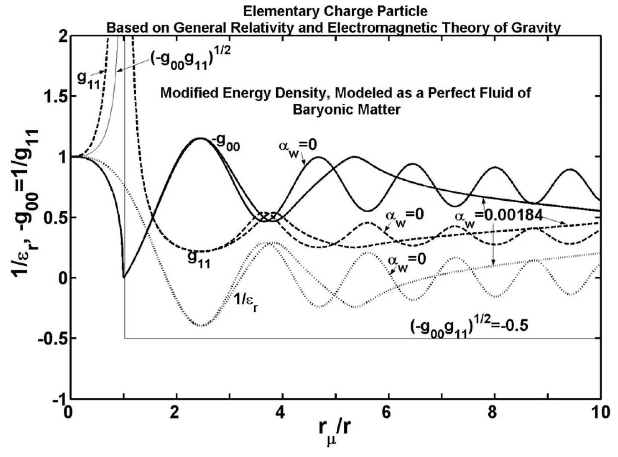
6.2. Modified Energy Density, Modeled as a Perfect Fluid of Conventional Baryonic Matter
It is not certain if the additional part of the modified electromagnetic energy density in (36) is to be treated in the same manner as the conventional electromagnetic energy density, as implemented in (29,30), or as conventional baryonic matter in the form of a perfect fluid [13]. The following formulations are established to model a perfect fluid with a general distribution of energy density , that maybe specifically applied to model the additional part of the modified electromagnetic energy density in (37). The basic formulations of the Christoffel symbols and Ricci elements of (7-11) will be used here as the starting point of the derivation, leading to the following relations.
Given inverse-relative permittivity distribution , independently solved from (2,39) for a given energy/mass distribution, the two equations - the relationship (6) of the two variables and with the known , and the above relationship (46) for the same two variables - maybe numerically (by trial iterations) solved for the two variables and (and hence ) for a general problem. Analytical solution maybe possible for a simple mass/energy distribution.
6.2.1. Validation of the Model with Schwarzschild Solution Internal to a Uniform Spherical Body
As an illustration/validation of the theory for a simple case, we will analytically derive Schwarzschild solution inside a body of mass M and radius , with a uniform mass-density = , following the procedure prescribed above. We will start the derivation with simple solution for the in this case, satisfying (1,2), and then solve for and as prescribed above. The results maybe verified with known solutions from the Schwarzschild metric in the internal region of the body [13,27].
Note that, as mentioned in Section 3.1, the mass M needs to be properly defined by integrating the distribution of the body’s conventional mass , which is defined in an ideal free space, weighted by the local inverse relative permittivity distribution . Accordingly, the uniform positive mass density assumed here would refer to uniformity of the weighted mass density, not of the conventional mass density defined in an ideal free space. That may not always be physically realistic if the resulting solution for the is negative, in which case the weighted mass density would be negative, contradicting the uniform positive density originally assumed.
Using the above expression of in the top line equation, is solved as follows.
The modeling of a conventional baryonic matter as a perfect fluid, now validated for a neutral mass distribution, is then applied for the energy distribution of an elementary charge, with its modified definition of the energy density proposed at the beginning of the Section 6. The distribution associated with the modified energy density, solved in the sub-Section 6.1, with proper choice of the parameter constant for in (38), would apply for the present modeling of the modified energy density as baryonic matter. Using the given in (39), the metric elements and are solved by numerical iterations of the equations (6,46), as prescribed earlier, and are plotted in Figure 7 (noted with ). It maybe noticed, the solutions for the and in Figure 7 exhibit a singularity (radial derivative → ∞) at radius . For radii smaller than the singular location, there is a definite real solution for the equation (46) with , which maybe substituted in (6) to derive (and hence ) using the given in (39), by enforcing continuity of at the singularity. The same normalized mass in Figure 6, derived in (41) using the given , applies as well for the present modeling.
6.3. Higher-Order Dependence of the Modified Energy Density
In the modeling of the above Section 6.1, Section 6.2, the modified energy density = (see (36)) was defined, with the function U in the dominant, new part proportional to the original energy density (see (37)), as a simple first order approximation. The resulting stable mass , its equivalent classical radius , and the parameter , were related to each other in (43) by a dimensionless constant = , which was found to be suspiciously close to the inverse-fine structure constant = . Suspecting that the actual value of the dimensionless constant be exactly equal to , we anticipate that the small difference between the constant , derived based on the above first-order modeling, and , would be adjusted by a more rigorous treatment with a higher-order dependence of the modified energy density.
where the dimensionless parameter , or equivalently the energy-density parameter , represents a suitable second-order dependence of the function on the energy density . The effective inverse-relative permittivity is expressed in terms of the inverse-relative permittivity , as defined in (29).
Introducing the above revised expression (50) of the modified energy density in (37,38), the derivations of Section 6.1, Section 6.2 maybe repeated, in principle, in order to revise the results of Figures and for inverse-relative permittivity , normalized mass , and the metric elements and . However, the solutions may not be feasible analytically. Instead, we first revise the solution for from (37-39), with the revised expression (49) of . Accordingly, a differential-integral equation for is established, with two normalized variables and , as formulated in (50), which is numerically solved using a finite-difference/element technique. Note that the charge q is treated in (49,50) as a variable, with its maximum value equal to an elementary (electron) charge . The corresponding normalized variable is = =, with its maximum value equal to one. Whereas, the , as defined in terms of q in (39), is treated in (49,50) as a constant parameter evaluated at the maximum value of . All the derivations of the Section 6.1, Section 6.2 can now be revised, in terms of the numerically revised solution for ≡ .
The effective function , as defined in (29), is revised in terms of the revised solution for . Using the revised , the normalized mass of (41) is then revised, computed numerically as a double-integration of , with respect to both the normalized variables and .
Using (51), the lowest stable mass of Figure is successfully revised to a slightly lower value, from to , by adjusting the parameter in (49,50). Accordingly, the resulting dimensionless constant in (43) is revised lower, to be precisely equal to the inverse-fine structure constant . This is a remarkable development, which would precisely trace the physical origin of the fine-structure constant to the new gravitational model of the elementary charge, with the modified energy density presented here.
The revised results of inverse-relative permittivity , normalized mass , and the metric elements and , for the special value , are plotted in Figure 6 and Figure 7, as a function of the normalized variable = . These are plotted together with respective results from the approximate first-order modeling in Section 6.1, Section 6.2, that are associated with , for a comparative study.
The second-order expression (49) of the gravitational field would start to deviate from the simple first-order expression = at energy density larger than the threshold level . This is associated with a distance r from the center of an elementary charge , less than a normalized threshold radius , as expressed in (49), assuming . Accordingly, for the specific value of we have found in Figure 6, this threshold radius for the onset of the second-order expression of (49) can be calculated to be , where from (42,43) is the classical radius associated with a static electron.
7. Discussion and Conclusion
New complementary formulations to model an elementary charge particle, combining general relativity and an electromagnetic theory of gravity, were studied, with alternate definitions of energy density and the related stress-energy tensor. These include the conventional definition of the energy density in an ideal empty space, for reference, and new corrected and modified definitions using an equivalent permittivity distribution for the empty space. The solutions for the metric-tensor elements are verified with existing reference solutions. It is recognized that the empty space, modeled by an equivalent permittivity distribution, be properly treated as a non-linear medium, in order to successfully develop self-consistent solutions for an elementary charge, with a physical stable structure. In contrast, the Reissner-Nordstrom solution, that uses the conventional model of energy density in an ideal empty space, would lead to an unstable structure of the charge. A corrected version for the Reissner-Nordstrom solution, where the energy density is modeled using an equivalent linear-permittivity distribution of the empty space, allows only a quasi-stable structure (as defined in Section 4.2). The quasi-stable behavior, although may not represent a physically realistic charge structure, the associated energy/mass may be of theoretical interest as a reference value for other related models. A further revised version of this analysis, but now with the energy density defined using a non-linear model for the equivalent permittivity distribution of the empty space, in fact leads to fully stable charge structures (as defined in Section 4.2) for discrete values of the charge radius. However, the resulting level of the stable energy/mass, with the lowest possible value (about same level as the above quasi-stable case), is much larger than the energy/mass of any known physical charge particle. Therefore, other than of special theoretical interest, as theoretically valid values of energy/mass of a self-consistent, stable charge structure, it is doubtful if any physical charge structure of nature represents such a stable solution.
This led us to seek other possible formulations, based on new modified definitions of energy density, which may allow stable solutions for an elementary particle with much lower levels of mass/energy. It is recognized that a definition of energy density in an empty space is theoretically non-unique, and therefore a suitable modified definition might exist that more rigorously represents physical nature, as compared to the conventional definition assuming an ideal empty space, or its corrected versions discussed above.
Solutions for the metric tensor elements, and the associated energy/mass of stable charge structures were derived, using modified definitions of the energy density. A first-order modified model is introduced, which is equivalent to an additional gravitational field proportional to the original energy density, with constant of proportionality as a new parameter. By associating the stable solution, with the smallest possible mass/energy, to a static electron without spin, the constant is estimated to be about 600 , declared as a new fundamental physical constant of nature. More fundamentally, the constant , the resulting smallest stable mass , and the associated classical charge radius , are related to each other by a dimensionless constant = , which is numerologically close to the inverse fine-structure constant = of quantum electrodynamics. This strongly suggests that the proposed theory is possibly the physical basis of the fine-structure constant. However, the small difference between the dimensionless constant derived from the presented theory and the fine structure constant which is based on accurate measured data, is intriguing, suggesting that a more accurate model is needed to bridge the small difference. Accordingly, a more rigorous modified model is studied, by expressing the additional gravitational field with an appropriate higher-order dependence on the original energy density.
A suitable second-order model is successfully formulated and numerically implemented using a finite-difference/element technique. As anticipated, the model results in a somewhat reduced particle mass ( = ), as compared to that ( = ) from the original first-order model, so that the new adjusted dimensional constant precisely matches the inverse-fine structure constant =. This is a significant development, towards precisely tracing the physical origin of the fine structure constant through the new theory. Further, the two values of , before and after the adjustment from the new higher-order model, may carry independent physical significance in finer estimation of the electron’s g-factor.
Upon definitive resolution of the modified general-relativistic formulations, specifically for the case of a static elementary charge, the complete formulations would provide a rigorous analytical framework to model a complete electrodynamic structure of a spinning elementary charge. The same analytical framework may also be extended, in principle, to model static or dynamic structures of other elementary charge particles (proton, muon).
References
- Einstein, A. Zur allgemeinen Relativitdtstheorie (On the General Theory of Relativity), also see Addendum pp.799-801. Preussische Akademie der Wissenschaften, Sitzungsberichte (Part 2) 1915, 778–786. [Google Scholar]
- Einstein, A. Grundlage der allgemeinen Relativitätstheorie (The Foundation of the General Theory of Relativity). Annalen der Physik 1916, 354, 769–822. [Google Scholar] [CrossRef]
- Newton, S.I. Principia: Mathematical Principles of Natural Philosophy; Cohen, I. B., Whitman, A., Budenz, J., Eds.; University of California Press, 1999. [Google Scholar]
- Newton, S.I.; Hawking, S. Principia; Running Press, 2005. [Google Scholar]
- Einstein, A. Erklärung der Perihelbewegung des Merkur aus der allgemeinen Relativitätstheorie (Explanation of the Perihelion Motion of Mercury from the General Theory of Relativity). Preussische Akademie der Wissenschaften, Sitzungsberichte (Part 2) 1915, 831–839. [Google Scholar]
- Dyson, F.W.; Eddington, S.A.; Davidson, C. A Determination of the Deflection of Light by the Sun’s Gravitational Field, from Observations Made at the Total Eclipse of May 29, 1919. Philosophical Transactions of the Royal Society of London 1920, 220, 291–333. [Google Scholar]
- Wikipedia. Einstein field equations. 2022. Available online: https://en.wikipedia.org/wiki/Einstein_field_equations.
- Reissner, H. Uber die Eigengravitation des elektrischen Feldes nach der Einsteinschen Theorie. Annalen der Physik (in German). 1916, 50, 106–120. [Google Scholar] [CrossRef]
- Wikipedia. Reissner-Nordstrom metric. 2021. Available online: https://en.wikipedia.org/wiki/Reissner_Nordstrom_metric.
- Wilson, H.A. An Electromagnetic Theory of Gravitation. Physical Review 1921, 17, 54–59. [Google Scholar] [CrossRef]
- Feynman, R.P.; Leighton, R.B.; Sands, M. Lectures on Physics Vol.II, Ch.28; Addision Wesley, 1964. [Google Scholar]
- Schwarzschild, K. Uber das Gravitationsfeld eines Massenpunktes nach der Einsteinschen Theorie [On the gravitational field of a point mass following Einstein’s theory]. In Sitzungsberichte der Koniglich-Preussischen Akademie der Wissenschaften [Prussian Academy of Sciences, meeting reports (Part I)]; (in German). 1916; pp. 189–196. [Google Scholar]
- Schwarzschild, K. Uber das Gravitationsfeld einer Kugel aus inkompressibler Flussigkeit nach der Einsteinschen Theorie [On the gravitational field of a ball of incompressible fluid following Einstein’s theory]. In Sitzungsberichte der Koniglich-Preussischen Akademie der Wissenschaften [Prussian Academy of Sciences, meeting reports (Part I)]; (in German). 1916; pp. 424–434. [Google Scholar]
- Brodsky, S.; Franke, V.; Hiller, J.; McCartor, G.; Paston, S.; Prokhvatilov, E. A Nonperturbative Calculation of the Electron’s Magnetic Moment. Nuclear Physics B 2004, 703, 333–362. [Google Scholar] [CrossRef]
- Das, N. A Unified Electro-Gravity Theory of a Spinning Electron, and the Fundamental Origins of the Fine Structure Constant and Quantum Concepts. Paper Y15.0004; American Physical Society April 2020 Meeting. 2020. [Google Scholar]
- Das, N. A New Unified Electro-Gravity Theory for the Electron, and the Fundamental Origin of the Fine Structure Constant and the Casimir Effect. Journal of High Energy Physics, Gravitation and Cosmology 2021, 7, 66–87. [Google Scholar] [CrossRef]
- Carroll, S.M. Spacetime and Geometry: An Introduction to General Relativity; Cambridge University Press, 2019. [Google Scholar]
- Wald, R. General Relativity; The University of Chicago Press, 1984. [Google Scholar]
- Wikipedia. Derivation of the Schwarzschild solution. 2021. Available online: https://en.wikipedia.org/wiki/Derivation_of_the_Schwarzschild_solution.
- Harrington, R.F. Time Harmonic Electromagnetic Fields; McGraw-Hill Co., 1984. [Google Scholar]
- Will, C.M. The Confrontation Between General Relativity and Experiment. Living Review of Relativity 2006, 9. [Google Scholar] [CrossRef] [PubMed]
- Gorelik, G. First Steps of Quantum Gravity and the Planck Values: Studies in the History of General Relativity. In Einstein Studies; Eisenstaedt, J., Kox, A. J., Eds.; Boston University, 1992; Volume 3, pp. 364–379. [Google Scholar]
- Wikipedia. Electromagnetic stress-energy tensor. 2022. Available online: https://en.wikipedia.org/wiki/Electromagnetic_stress_energy_tensor.
- Handbook of Mathematical Functions: Bessel Functions of Integer Order; Abramowitz, M., Stegun, I., Eds.; Cambridge University Press, 1964. [Google Scholar]
- Wikipedia. Fine-structure constant. 2017. Available online: http://en.wikipedia.org/wiki/Fine_structure_constant.
- Sommerfeld, A. Atomic Structure and Spectral Lines; Brose, H. L., Translator; Methuen, 1923. [Google Scholar]
- Wikipedia. Interior Schwarzschild metric. 2021. Available online: https://en.wikipedia.org/wiki/Interior_Schwarzschild_metric.
Figure 1.
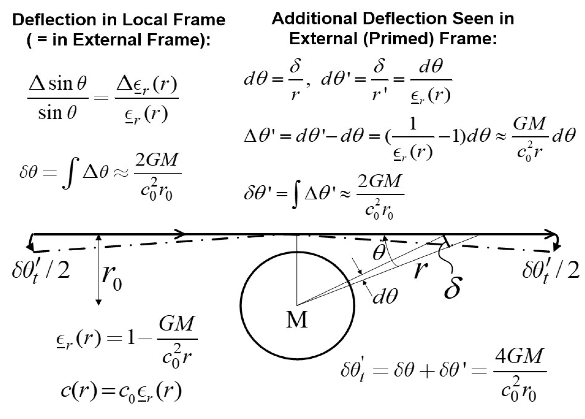
Figure 2.
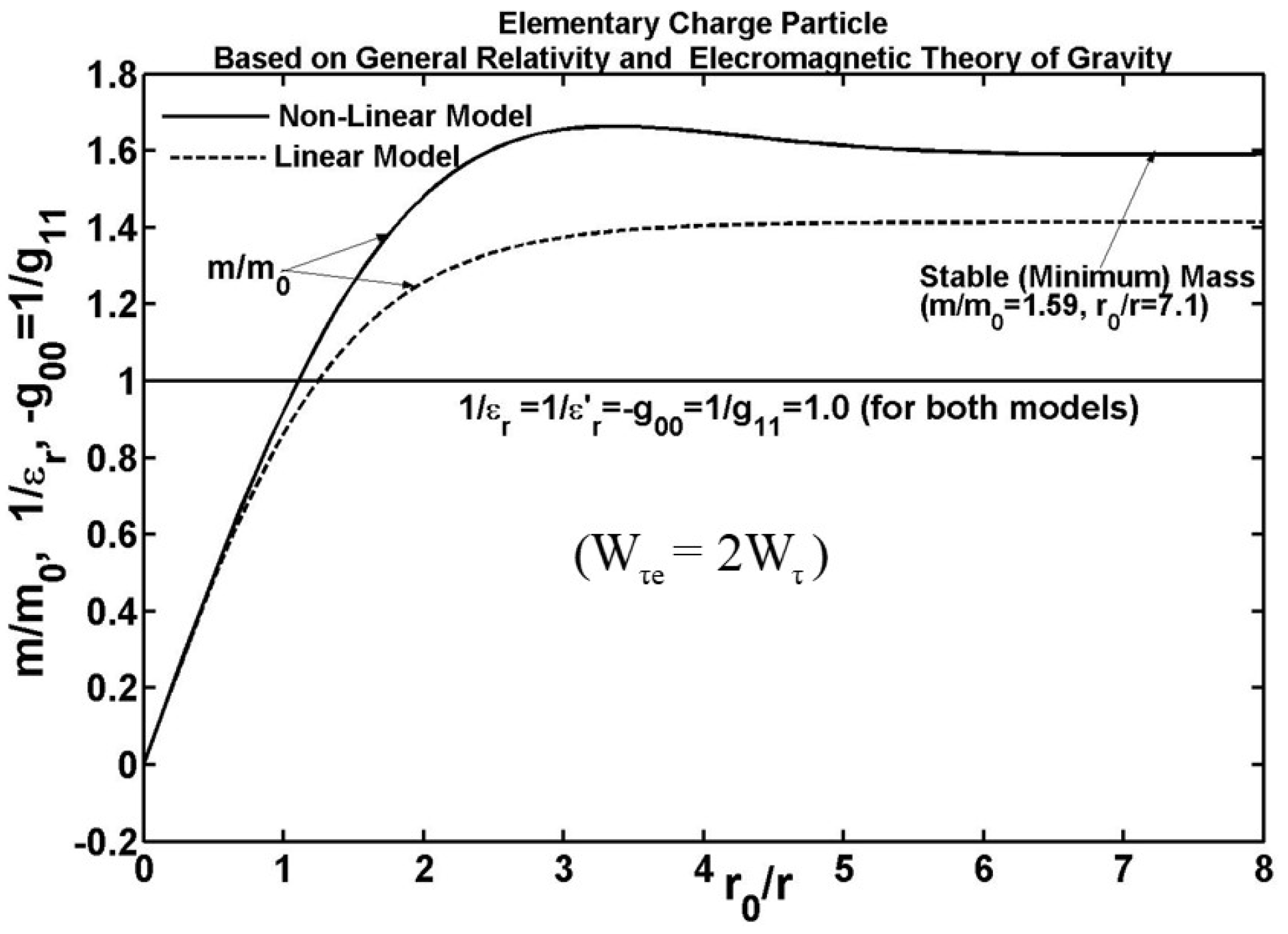
Figure 3.
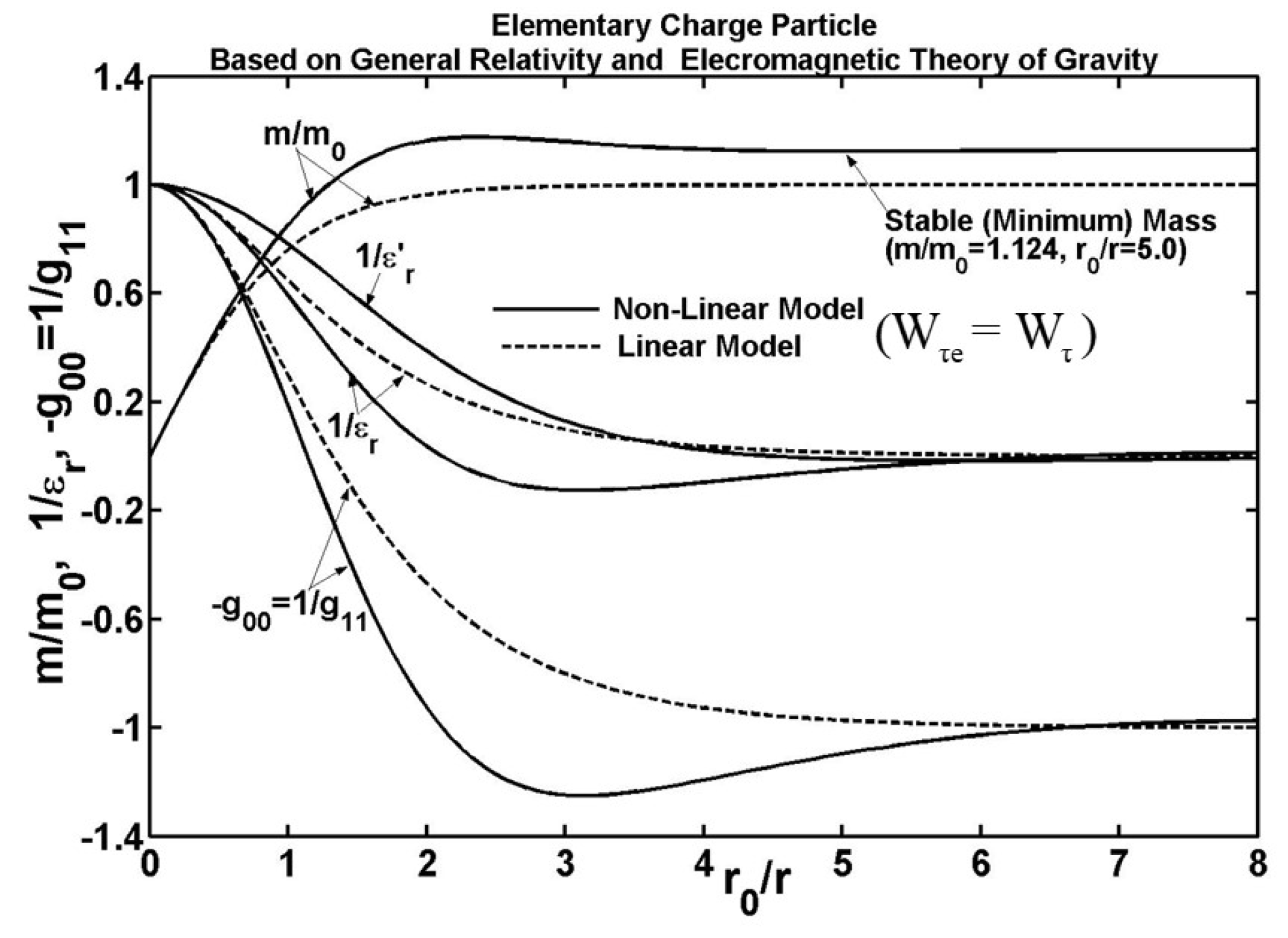
Figure 4.
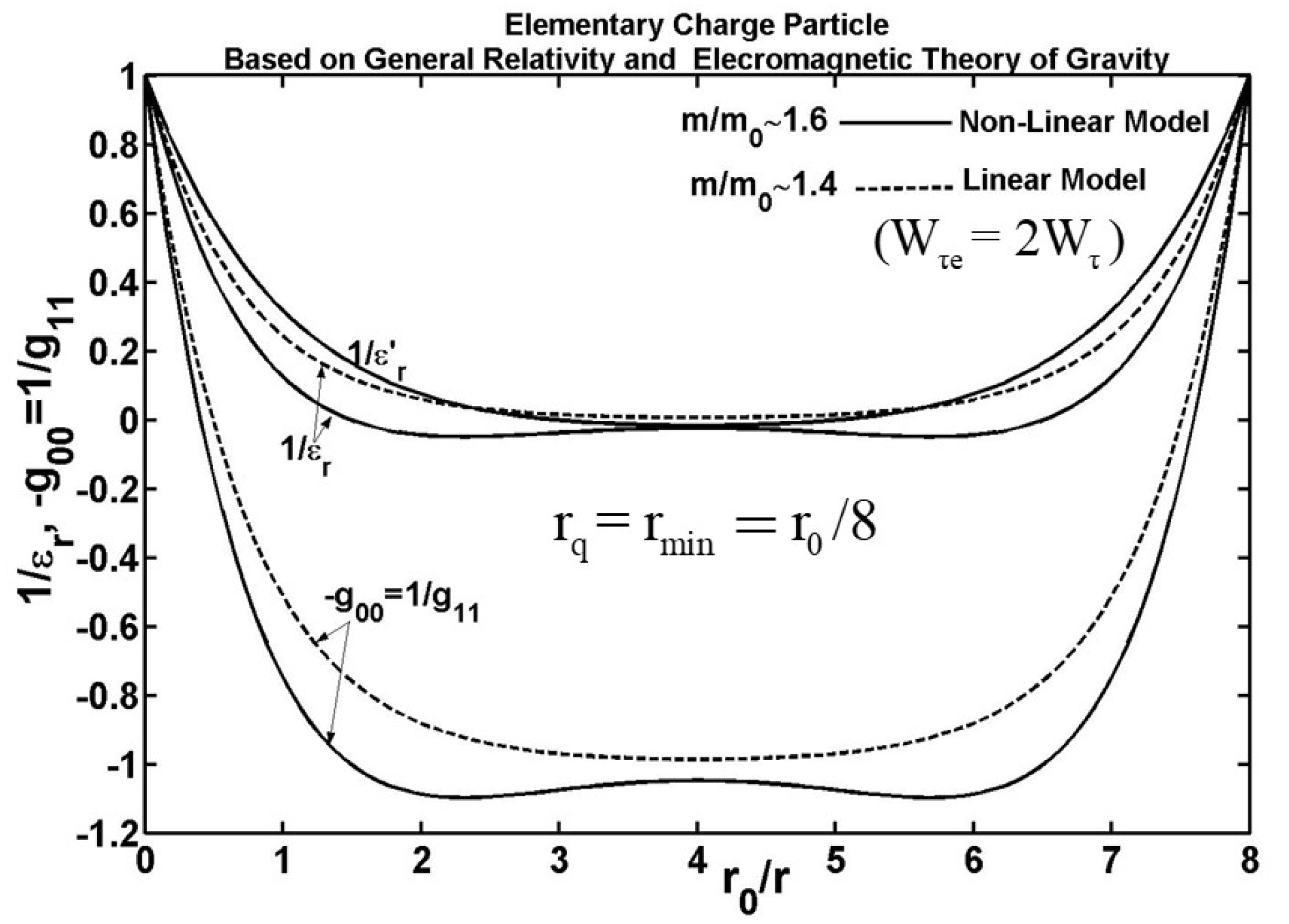
Figure 5.
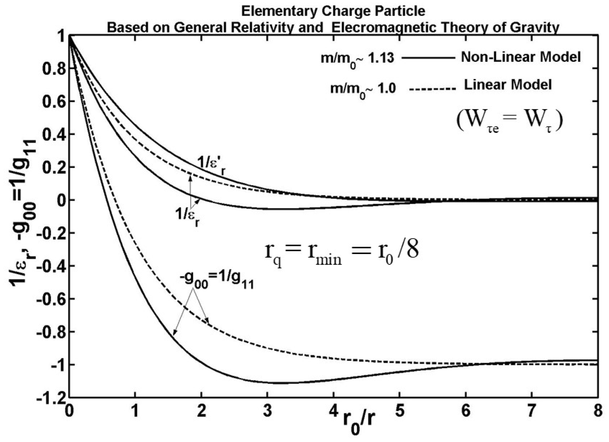
Figure 6.
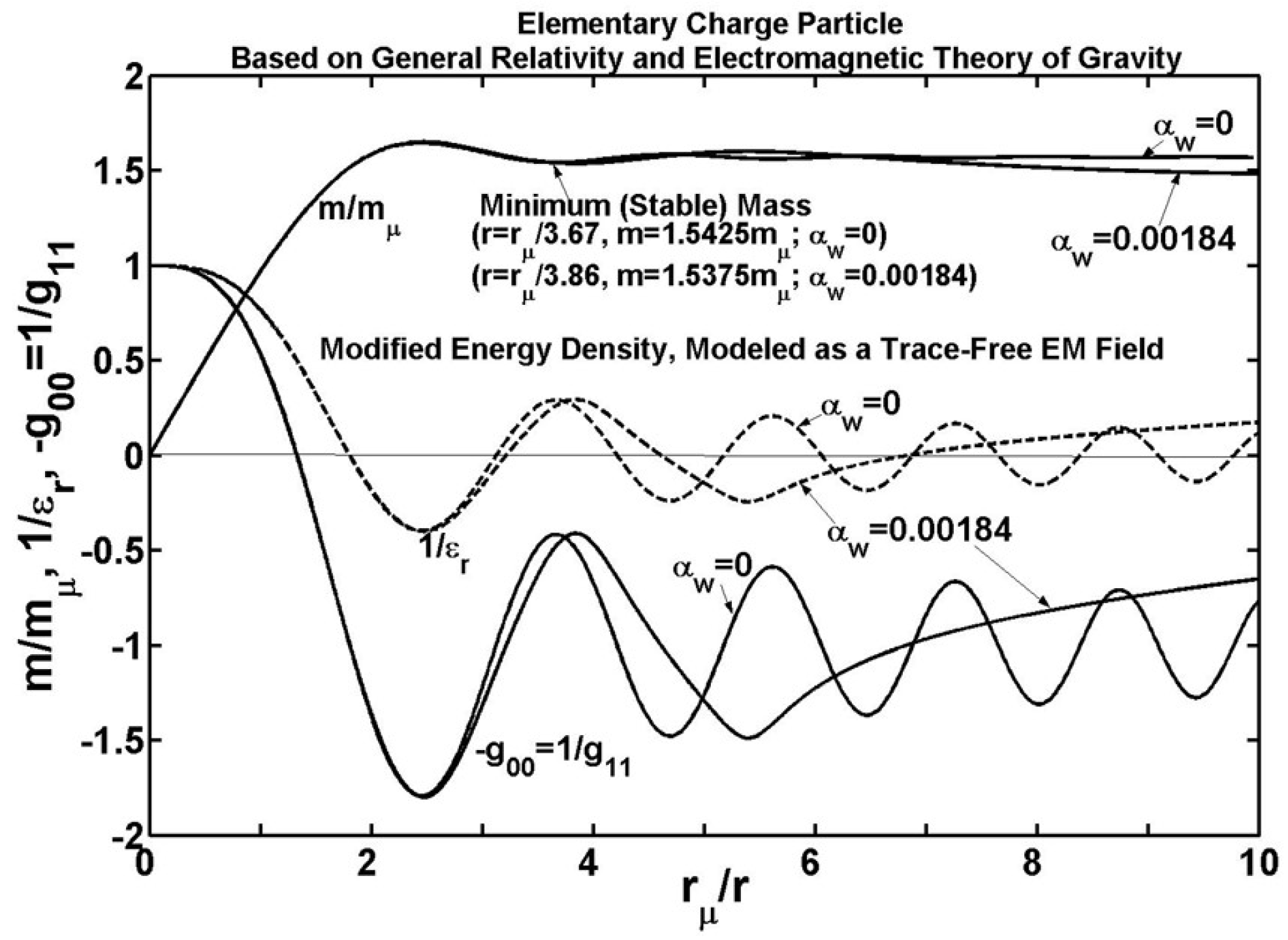
Figure 7.
Disclaimer/Publisher’s Note: The statements, opinions and data contained in all publications are solely those of the individual author(s) and contributor(s) and not of MDPI and/or the editor(s). MDPI and/or the editor(s) disclaim responsibility for any injury to people or property resulting from any ideas, methods, instructions or products referred to in the content. |
© 2026 by the author. Licensee MDPI, Basel, Switzerland. This article is an open access article distributed under the terms and conditions of the Creative Commons Attribution (CC BY) license.
Copyright: This open access article is published under a Creative Commons CC BY 4.0 license, which permit the free download, distribution, and reuse, provided that the author and preprint are cited in any reuse.


