Submitted:
08 January 2026
Posted:
09 January 2026
You are already at the latest version
Abstract
Above ground storage tanks are used to store various fluids and chemicals for many industrial purposes. According to API standard 653, the structural integrity of these tanks must be regularly assessed. The U.S. EPA requires each operator to have a Spill Prevention, Control and Countermeasure Plan (SPCC) for aboveground storage con-tainers. The accepted practice for inspection of these tanks, particularly the tank bot-toms, involves removing the tank from service, emptying the tank, and inspecting di-rectly from the interior. The required inspection operations are hazardous due to the chemicals themselves as well as the requirement to operate within confined spaces. An inspection from outside the tank would have significant cost and time benefits and would provide a large reduction in the risks faced by the inspection personnel. Guided wave (GW) testing is one promising candidate for screening of storage tanks walls and bottoms from the tank exterior due to the ability of GWs to propagate long distances from a fixed probe location. The lowest order transverse-motion guided wave modes (e.g., torsional vibrations in pipes) are a good choice for long-range inspection because this mode is not dispersive; therefore, the wave packets do not spread out in time. A common weakness of guided wave inspection is the complexity of report generation in the presence of multiple geometry features in the structure, such as welds, welded plate corners, attachments and so on. In some cases, these features cause generation of non-relevant indications due to mode conversion. Common non-relevant indications are described in this paper. Another significant challenge in applying GW testing is development of probes with high enough signal amplitudes and a relatively small footprint to allow them to be mounted on relatively short tank bottom extensions. In this paper a new generation of magnetostrictive transducers will be presented. The transducers are based on a reversed Wiedemann effect and can generate shear hori-zontal mode guided waves over a wide frequency range (20 – 150 kHz) and with SNR in excess of 50 dB. The recently developed SwRI MST 8x8 probe contains an array of 8 pairs of individual magnetostrictive transducers (MsTs). The data acquisition hard-ware allows acquisition using Full Matrix Capture (FMC) and analysis software re-porting of anomalies based on Total Focusing Method (TFM) image reconstruction. This novel inspection package allows generation of reports containing high accuracy corrosion mapping information. Case studies of this technology on actual storage tanks walls and bottoms will be presented together with validation of processing methods on mockups with known anomalies and geometry features.
Keywords:
magnetostrictive transducer arrays
; guided wave testing
; storage tank inspection
; full matrix capture
; total focusing method
1. Introduction
Typical industrial storage tanks range in diameter from 2.5 m to 100 m. There is a great variety of tank bottom geometries (lap welded, butt welded or both). Guided wave methods for inspecting the tank floor from the exterior have been investigated by different research groups for at least a decade. An array of piezoelectric transducers placed around the annular skirt plate was used to receive a tomographic image of lap welded tank bottom condition in [1]. The attenuation profile of 50 kHz lowest order symmetric mode (S0) mode guided wave was used to reconstruct an 8-m diameter tank bottom condition, but the accuracy limits were not determined. Other research indicated that a similar tomography approach could be utilized for finding 100 mm diameter 50% deep anomalies. The researchers placed 48 transducers around a 4.1 m diameter tank bottom mockup [2]. A magnetostrictive guided wave probe in pulse-echo configuration to scan the tank floor by moving the probe along the outside skirt plate was reported in [3]. Wall thinning and pit holes were successfully detected with the help of Synthetic Aperture Focusing Technique (SAFT) processing. Anomalies were detected in annular ring area (before the first lap weld). A method utilizing higher order modes cluster (HOMC) guided waves for online defect detection in the annular plate region of above-ground storage tanks was reported in [4]. The method is applicable for corrosion mapping in the region of one meter and less from the vertical wall with a probe positioned outside of the tank. Another method of anomaly detection in storage tank floors was based on placing guided wave probes on storage tank walls [5]. It was found that shear horizontal (SH) guided wave modes provided superior signal to noise ratio compared to the S0 mode in the tank floor. Damage detection in hazardous waste storage tank bottoms using ultrasonic guided waves was reported in [6]. Detection was accomplished using an SH0 mode guided wave EMAT crawler in the frequency range of 45 – 64 kHz in a butt-welded tank bottom. Penetration capability of S0 mode in lap welded tank bottoms was reported in [7]. It was shown that guided waves in the frequency range of 20 – 40 kHz provided the best penetration. Bottom plate damage localization based on dual array SH0 mode piezoelectric sensors installed on the tank bottom extension and also on the tank wall was reported in [8]. It was shown that utilizing the dual array helped to eliminate non-relevant indications produced by piezoelectric transducers.
The guided wave methods relevant to tanks inspection can be split into two groups – methods targeting long-range coverage at the cost of lower sensitivity, and methods providing shorter range coverage (mostly in the area before the first lap weld), but delivering more accurate defect information.
The research presented in this paper will focus on corrosion mapping in the area before the first lap weld. In the case of butt-welded tank bottoms or walls, the range of coverage could be much longer (20 plus meters).
2. Magnetostrictive Sensors
The physical effect for generation of transverse vibration using orthogonally oriented static and variable magnetic fields was discovered by Wiedemann for generation of torsional motion in rod shaped components [9]. In a similar evaluation on a plate, an SH wave transducer consisting of a meander coil and static bias magnetic field parallel to the coil elements was described by Thompson in 1979 [10]. In this configuration, the SH wave propagated in the direction perpendicular to the static magnetic bias direction. In an alternative design, the static and pulsed fields are reversed, and the SH wave propagated in the direction parallel to the static magnetic bias; this method was called the reversed Wiedemann effect [11,12]. For practical NDE, increased signal amplitudes is always a way to accomplish better coverage and sensitivity. This is why both effects have been implemented using a soft ferromagnetic patch material (typically nickel or FeCO alloy) that has a much greater magnetostrictive effect than typical structural metals [13,14,15]. Figure 1a shows an example of such a patch attached to a tested structure. In this example, two mutually orthogonal coils are wrapped around the patch, one parallel to patch rolling direction (Y direction) and another perpendicular to it.
In this arrangement, one coil provides a time varying magnetic field and the other coil provides a permanent magnetic bias, with both coils generating in-plane magnetic fields. It was experimentally confirmed that as long as the wave propagates perpendicular to the patch rolling direction, the signal amplitudes generated are similar regardless of which coil operates as the pulsing coil. As an example, Figure 1b shows the reflection from the plate end produced by a 25 x 25 mm FeCo patch with coil 1 pulsing and coil 2 providing magnetic bias (black trace) and coil 2 pulsing and coil 1 providing magnetic bias (red trace).
The wave amplitude is influenced by the aspect ratio of the patch. For example, if direction Y is the desired propagation direction, making the patch longer in the X direction makes the signal amplitude propagating in the Y direction higher and the sideways portion of energy (direction X) will be reduced.
In addition to SH0 modes propagating sideways, compressional S0 mode waves propagating through 35°–215° and 320°–140° axes can be observed. This portion of energy is shown in Figure 1a with blue arrows. Figure 2 shows results of vibration readings from a 304 x 304 mm aluminum plate with an SH0 mode probe with a 65 mm aperture acoustically coupled to one side of the plate. It can be clearly seen on that together with the wanted SH0 mode, S0 mode is also generated, in addition to SH0 modes going sideways and creating additional waves (shown in Figure 2c). It should be noted that the patch can also detect the unwanted modes or energy propagating in one of these unwanted directions. This is why each particular probe design typically goes through a calibration process on mockups to characterize energy generation for desired and undesired modes and side-effects specific to each probe geometry.
Figure 3 shows the principal design of a reversed Wiedemann effect MsT probe. Major components of the MsT probe include two 12.7 mm wide and 76 mm long FeCo strips installed next to each other for applying direction control to the guided wave pulse. The probe is elongated in the rolled direction of the FeCo strip to reduce generation of unwanted wave modes. A coil wound around each strip provides the pulsed field, and a belt of small rare-earth magnets is placed on top of the strip to achieve uniform and self-sustained biasing magnetization in the wave propagation direction.
The entire sensor assembly is encapsulated into a flexible urethane coating to protect all components from environmental impact and for durable operation. The probe is sized to fit it to tank bottom extensions as short as 20 mm.
3. Magnetostrictive Array Probes
The next step in MsT technology evolution is based on an array of sensors and advanced data collection and postprocessing algorithms. Figure 4 shows an MsT 8x8 probe with 8 MsT segments constructed as described above. The probe has flexible joints between segments that let it be bent around a large radius in any direction. Each segment is individually connected to a SwRI MsSRV5M guided wave instrument with integrated multiplexer. This instrument provides pitch-catch and pulse-echo data collection methods from every possible combination of sensor segments. The probe can be installed on the tank bottom extension or tank wall using a magnetic clamping fixture. Figure 4a shows the field deployable MsSRV5M instrument with an MsT 8x8 array probe. Figure 4b,c show the probe installed on the tank bottom extension and on the wall of a large storage tank. Water soluble shear wave couplant is used to facilitate acoustic coupling of the probe.
4. Data Acquisition
Three different methods of data collection can be used with the 8x8 probe:
- ○
- Synthetic aperture focusing technique (SAFT): each segment used as a pulser/receiver pair
- ○
- Common source method (CSM): all segments pulsed simultaneously, and each segment receives
- ○
- Full Matrix Capture (FMC) mode: all possible segment combinations are used for pulsing and receiving
Figure 5 illustrates the available data acquisition protocols and the number of data sets collected in each case.
The data acquisition time will vary depending on the acquisition method selected. For SAFT and CS, data collection of 8 waveforms in both directions is typically approximately 20 sec. For TFM (FMC collection mode) the average acquisition time is about 3 minutes for 64 waveform pairs.
Figure 6a shows an example of a reconstructed image of anomalies in a mockup plate using these three methods. The MsT 8x8 probe was mounted on the edge of a 6.4 mm thick carbon steel plate at a distance of 6 meters from target anomalies. The objective of this test was to demonstrate the ability of the probe and processing algorithm to detect and locate anomalies at a long distance from the sensor. Three EDM notches were introduced in the plate, with depths of 1.3 mm and 2.5 mm. Figure 6a shows that all three anomalies could be clearly localized from more than 6 meters away using the TFM method, including one 2.5 mm deep notch positioned past a butt weld. The test frequency was 180 kHz. Differences in anomaly imaging using TFM, CSM, and SAFT are presented in Figure 6. In summary, the TFM image produced the best anomaly localization and better detection of the smallest anomaly – the 1.3 mm deep notch.
Another example of long-range coverage is shown in Figure 7. The figure shows a TFM-reconstructed image of a 43 m high storage tank wall obtained at 30 kHz using an MsT 8x8 probe mounted on the tank bottom extension. This tank had lots of generalized corrosion - only 30 kHz provided good range of coverage in the wall. Multiple horizontal butt welds in the tank wall were clearly imaged up to the 30-meter height. The TFM algorithm was able to provide lateral localization of defects up to the 9-meter mark (Indication 1). Past this distance, the lateral localization of the defect was difficult due to the large beam spread at relatively low frequency. However, the axial position of the suspect indication (Indication 2) could still be reported. at the 28 m distance mark.
More accurate anomaly mapping at greater distances would require using probes with wider segments or higher frequencies (if applicable).
5. Challenges of Tank Bottom Inspection Using Guided Waves
The most common challenges of thank bottom inspection from the exterior are listed below:
- ○
- Uneven and sometimes heavily rusted tank extension surface
- ○
- Small tank extension (less than 25 mm to mount the probe)
- ○
- Guided wave energy leaking into the vertical wall of the tank
- ○
- High attenuation of guided waves in the presence of generalized corrosion, deposits, or liners
- ○
- Great variety of tank bottom geometries (lap welded, butt-welded or both, patches and penetrations) and the absence of tank geometry configuration documentation
- ○
- Presence of multiple areas with difficult access to the tank bottom extension due to other geometry features
Figure 8 shows a typical tank bottom geometry with the guided wave probe mounted on the tank bottom extension on a, along with some sample data from acquired from butt-welded tank bottom on b.
Guided wave energy leaking into the vertical wall is hard to avoid due to welded joints. It results in merging indications produced by the bottom and wall. Figure 8b shows an A-scan obtained from a 10-meter diameter storage tank with hydrofluoric acid and with a liner covering the tank bottom. Data acquired at 65 kHz are rectified positive, and data acquired at 120 kHz are rectified negative. As can be noted from the figure, 120 kHz SH0 mode GW provided full penetration through the entire bottom plate. Some artifacts produced by welds in the vertical wall could be observed at 2.8 and 5.6 m. The lower frequency provided much more pronounced reflections from horizontal welds in the vertical wall, but GWs at this frequency did not reach the opposite side of the tank bottom. The bottom plate of this tank was 7 mm thick; the vertical plate thickness near the tank bottom was 12.7 mm. It should also be noted that for a given thickness of vertical wall (12.7 mm), the dead zone past the wall was 11 cm at 120 kHz and 18 cm for 64 kHz. The dead zone might be longer or shorter depending on the thickness of the vertical plate. Indication originating from the wall could be tracked down either by sweeping the frequency of GW or, 8x8 probe could be placed on vertical wall at different elevations providing GW inspection of the wall condition. The final report is provided with an option of merging indications on a sketch of a tank.
For welded tank bottoms, GW inspection will perform the best in the area before the first lap weld. Some GW energy penetration is possible past the first lap weld, but the detection capability will be much lower in this region. Examples below will focus on performance in lap welded tank bottoms.
6. Mockup Tests
To determine the performance of the 8x8 probe, two mockups were fabricated. One mockup was a 260x210x7 mm carbon steel plate. Another mockup was a simulation of a lap welded tank bottom with attached vertical wall. Figure 9a shows the geometry of the first mockup with the probe positioned near the bottom edge, overlapped with the B-scan image. The probe was intentionally offset from the bottom of the plate to capture side reflections from the near edge located 7 cm from the probe segment 1. The test was conducted at 64 kHz; the resulting B-scan image was obtained using 8 segments. It can be noted that side A caused a diagonal trace of SH0 mode indications corresponding to side reflections produced by segments 1 – 8. Based on the distance (83 cm) of side indications produced by segment 8, the velocity of waves propagating to the sides was calculated to be 3230 m/s, confirming that these were SH0 mode waves. Assuming the end of plate to be a 100% reflector, the amplitude of these indications was 1.7%.
Another diagonal trace can be seen in the upper side of the B-scan. It has a different slope because it is an S0 mode reflection produced by plate corner C. Based on the position of this indication, it originated from an SH0 mode propagating to the plate corner at 3230 m/s and returning at 5400 m/s, which is the velocity of S0 mode for the frequency-thickness ratio (0.91) of the mockup. The maximum amplitude of this set of indications was 3% in comparison to the end reflection. Figure 9 also shows A-scans using transmitter-receiver pairs of segments S1-S1, S1-S2, S1-S3, and S1-S4. Arrival times for SH0 mode side reflections and S0 mode corner reflections are marked with dotted lines. With overall accomplished SNR at 53.9 dB at 64 kHz (based on comparison of plate end reflection and background noise), indications produced by these side effect seem to be rather small. They still need to be understood by the analyst in order to avoid false positives during field tests.
Another mockup was fabricated to provide more realistic tank bottom conditions. The mockup consists of three 6.4 mm thick plates that compose the tank floor and a single vertical 32 mm thick plate that represents the tank wall. The tank floor includes one lap weld that runs parallel to the tank wall and one seam weld that runs from the tank wall to the lap weld in the tank floor. The tank wall is joined to the floor by a fillet weld that runs along both edges of the vertical plate. A skirt with a width of approximately 25 mm extends beyond the wall. An illustration of the mockup portion used for the test is shown in Figure 10a. The 8x8 probe position is shown in Figure 10b. Two 10-mm diameter cone-bottom holes were introduced in the floor to simulate corrosion defects. The locations of both holes are highlighted with circles in Figure 10a. The depth of the 1st hole (pit 1) is roughly 28% of the wall thickness, and the depth of the 2nd hole (pit 2) was 56%.
The distance to both pits from the vertical wall is 0.78 m. The probe was positioned with segment 1 close to a butt weld in the middle of the bottom plate, as shown in Figure 10b. Pit 1 was in the area covered by segments 1 – 4; pit 2 was in the area covered by segments 5 – 8. Data were acquired using FMC with the full set of 8 segments (S1 – S8) and two separate subsets of 4 segments (S1-S4 and S5-S8). The reason for using two 4 segment arrays is that pit 1 is located in the aperture of the first 4 segments (S1-S4), and at the distance to the pits and for the known beam spread, the contribution of the other 4 segments when transmitting would be limited to detection of the lap weld only. On the reception side they still could collect some unwanted mode converted signals.
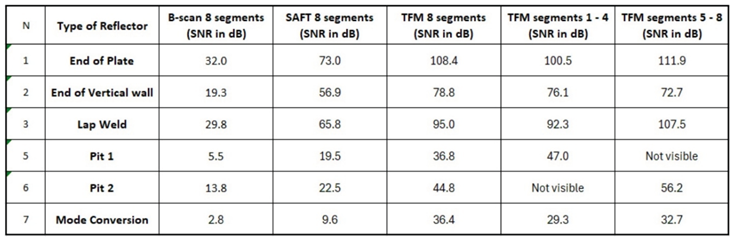
Figure 11 shows 5 reconstructed images obtained using a 90 kHz center frequency. An 8-segment B-scan image is shown in Figure 11a, 8-segment SAFT image in Figure 11b, 8-segment TFM image in Figure 11c, 4-segment TFM image utilizing segments S1 – S4 in Figure 11d, 4-segment TFM image utilizing segments S5 – S8 in Figure 11e. All plots were used to extract SNR information for geometry features, known defects and non-relevant (mode converted) indications. The list of tracked indications includes an end of the bottom plate, an end of the vertical plate, a lap weld, pit 1, pit 2, and a mode converted signal artifact. SNR values were calculated in reference to the noise floor and can be found in Table 1. Charts showing measured SNR for each indication is shown in Figure 12. Based on analysis of indication amplitudes, the following conclusions can be made:
- ○
- The B-scan using 8 segments (Figure 10a) produced a 5.5 dB SNR for pit 1 (28% deep) and 13.8 dB SNR for pit 2 (56% deep). The SNR of the lap weld was 29.8 dB versus 32 dB SNR for the bottom plate end. On a linear scale, the pit 2 amplitude was 2.5 times higher than pit 1 (versus a factor of 2 in cross sectional area). The mode converted signal SNR was 2.8 dB. This level was not much greater than the background floor noise and very unlikely to result in a false positive call. The top end of the vertical wall produced 19.3 dB versus 29.8 dB indication produced by the lap weld. This implies that only half of the energy propagating in the bottom plate leaked in the vertical wall. Indication span (width) information could be hardly guessed from B-scan image. However, amplitude ratio between reflection from the top of vertical wall (19.3 dB) versus reflection from pit 2 (13.3dB) seems to be realistic (2/1 in linear scale). This last factor is important because reflection from the first horizontal weld in the tank wall can be used as a reflection reference for calibration purposes.
- ○
- An 8-segment SAFT-scan (Figure 11b) produced 19.5 dB SNR for pit 1 and 22.5 dB for pit 2. The signal produced by mode conversion was 9.6 dB. In this case, pit 1 could be clearly detected at 9.9 dB higher amplitude over the nonrelevant indication. On linear scale, pit 2 amplitude was 1.4 times higher compared to pit 2 (versus actual 2/1 times amplitude ratio). The amplitude of indication produced by the lap weld was 65.8 dB compared to 73 dB amplitude produced by the bottom plate end. The top end of the vertical wall produced a 56.9 dB indication, implying that only 15% of the energy propagating in the bottom plate leaked into the vertical wall. This number is different than readings from the B-scan.
- ○
- An 8-segment TFM image (Figure 11c) produced 36.8 dB amplitude for pit 1 (28% deep) and 44.8 dB amplitude for pit 2 (56% deep). There is a significant improvement in SNR for pit detection using TFM. However, an artifact produced by the mode converted signal was 36.5 dB, which is close to the amplitude of pit 1 and could potentially be misreported as indication. On the linear scale, the pit 2 amplitude was 2.5 times higher compared to pit 1 (versus actual two times amplitude ratio). The indication produced by the lap weld was 95 dB versus 108.4 dB produced by the bottom plate end. The top end of the vertical wall produced a 78.8 dB indication. This implies that only 15% of the energy propagating in the bottom plate leaked into the vertical wall (this number is offset similar to results when using SAFT). In comparison to SAFT, TFM produced about 6 dB improvement in SNR for the localized pits. The lap weld and plate end SNRs increased by about 30 dB. At the same time, the amplitude of the mode converted indication increased by 6 dB. The significant reduction of the indication produced by the mode-converted signal was the reason to process TFM image using two 4-segments acquisitions.
- ○
- Figure 11d shows TFM reconstruction of data acquired from the first 4 segments, S1-S4. Segments 1 - 4 aligned well with pit 1. This pit produced 47 dB SNR, 10 dB higher than with all segments. Also, the pit 1 signal is now 8 dB greater than the 29.3 dB SNR produced by mode conversion instead of the approximately equal signal for all segments The reason for the improvement is better alignment of firing and receiving segments with anomaly location.
- ○
- Figure 11e shows TFM reconstruction from the second subset of 4 segments, S5-S8. These segments were aligned well with pit 2. This pit produced 56.2 dB SNR, 12 dB higher than with the 8-segment TFM reconstruction and 23.5 dB greater than the mode converted signal. SNR numbers for the plate end, lap weld and vertical wall indications are similar to those from the TFM image of the 8-segment acquisition.
- ○
- The amplitude ratio between pit 1 and pit 2 using segments 1-4 and 5-8, respectively, was 9 dB, a factor of approximately 2.8, vs. a cross-sectional area difference of a factor of 2.
In conclusion, the information obtained from testing on the mockup indicates the following:
- Signals leaking from the sides of the probe did not exceed 1.7% amplitude compared to the signals propagating in the desired direction at 64 kHz. This effect could be ignored on real tank bottom extensions due to the absence of sharp edges in actual tanks. This leakage amplitude is dependent on the test frequency and sensor design.
- Non-relevant indications due to the presence of S0 mode and mode conversion in corners produced indications of the order of 3% compared to the indications produced by the plate end. During testing on the realistic mockup, these indications were suppressed more effectively when using 8 segment SAFT or 4-segment TFM, compared to the reconstruction of the full set 8-segment FMC data.
- For a given scan length (area before the first lap weld), 4-segment TFM acquisition and processing produced better SNR than the 8-segment TFM.
- SAFT and TFM processing produced superior anomaly mapping information and SNR compared to B-scan imaging. An average of 30 – 40 dB SNR gain was accomplished for indications from anomalies and welds.
- The B-scan image produced more realistic amplitude ratios between anomaly indications and indication produced by the end of the vertical wall. This implies that initial amplitude calibration should be based on B-scan readings for more accurate defect sizing. This calibration information should be used for ranking of indications generated by SAFT or TFM algorithms.
7. Testing on Storage Tank
The majority of storage tanks have lap-welded bottoms. Figure 13a shows the bottom scheme of the tested storage tank and the position of the MsT 8x8 probe used for the test. The bottom plate was made of 8 mm thick A36 carbon steel. The first two vertical wall plates were 13.4mm and 12.6 mm thick, respectively. Due to the complexity of the tank bottom geometry and the blind zone behind the vertical wall (typically 11- 20 cm), some areas were uninspected, but this is a common weakness of any GW method. This tank was used for water storage for over 40 years; based on internal visual inspection, it had moderate to severe corrosion damage. The GW test procedure used was based on ASTM standard E2929-13 [16], which requires use of multiple test frequencies.
Figure 13b shows a TFM-reconstructed image at 64 kHz center frequency. The image contains indications from both the tank bottom and the wall. Welds in the wall could be clearly identified until weld 4 at 10 m distance from the probe. A corner of the lap welded joint in the tank bottom can be seen at 3 m. Circled areas have a number of indications likely related to corrosion. Horizontal wall scans (with the probe aligned vertically on the wall) in this area revealed the presence of only minor corrosion damage in the tank wall at this height, meaning that all moderate and severe corrosion could be attributed to the tank bottom. In case minor or severe corrosion was found, two plots (from tank bottom and tank wall) would have to be overlapped to clarify the origin of indications. Additional plots showing TFM imaging at 45 kHz (Figure 13c) and 32 kHz (Figure 13d) indicated that there is a cluster of significant corrosion pitting in the tank bottom.
It should be noted that the lower frequency also resulted in wider beam spread and larger coverage area of the bottom plate. This is the reason why area covered by indications appears to be wider on plot 13d compared to plots 13c and 13b.
Results of anomaly ranking in the covered area are shown in Figure 14. A corrosion region marked with the dotted line box can be seen in the 64 kHz data in Figure 14a. The first horizontal weld is at a vertical wall thickness reduction from 13.4 to 12.6 mm. This thickness change and the profile of weld crown could mean that there is a up to a 20% cross-section change at the weld. All other indications were ranked based on the indication 1 (marked as a reference weld). The maximum peak amplitude (57%) was detected at indication 3 located 30 cm from the probe. The indication closest to the probe was indication 2 located 20 cm from the probe. Three wall indications could be observed in Figure 13c at 45 kHz between 4 and 6 meters. The range of coverage at 30 kHz represented in Figure 13d was limited to 12 meters. The actual coverage of walls at this frequency reached 30 meters, as shown in Figure 7.
The reporting software also provides approximate anomaly width (span) and axial extent information. Anomaly 7 had the largest size (1.8 x 1.3 cm) and was ranked moderate based on the amplitude information. Ranking is performed based on the SNR values compensated for additional gain observed when using TFM versus B-scan (see the results in Table 1 for pits 1 and 2).
The time that it takes to acquire data depends on acquisition parameters such as number of averages, method of data collection, and acquisition length. For example, the time needed to acquire a typical dataset with 3 frequencies is 3 min for FMC/TFM and 1 minute for SAFT or Common Source methods. The time for data reconstruction depends on the acquisition method, reconstruction length, and test frequency. For example, reconstruction of a 20-meter image using TFM at 30 kHz takes about 0.5 minute on an 11th-generation i5-1145G7 processor with a 2.60GHz clock rate. These results allow reporting to be quickly performed immediately after the scan, to provide a quick determination if another method should be used for detailed characterization.
8. Conclusions
An 8-segment array of reversed Wiedemann effect MsT transducers can accomplish accurate corrosion mapping in storage tank bottoms and walls using SH0 guided waves. The data presented here addresses the side effects associated with transduction methods and contribution of unwanted S0 mode generation. The effects were assessed on mockups representing sides, corners, and a combination of butt and lap welds. It was shown that SAFT and TFM methods provide dramatic improvement in anomaly mapping and detection compared to simple A- and B-scans. However, in some cases, non-relevant indications from mode converted signals can appear with amplitudes similar to those of real defects and geometric features. It was shown that reducing the number of probe array segments to cover smaller areas could help reduce the amplitude of unwanted signals related to mode-conversion and improve the SNR of anomaly indications.
An anomaly ranking strategy was executed on a realistic mockup with a lap-welded bottom and a welded vertical wall using two simulated defects in the form of the drilled holes. It was shown that initial amplitude ranking information could be obtained from a B-scan using a horizontal weld in the vertical wall as a reference, while accurate anomaly location and width could be obtained from TFM images.
An example of indication ranking in storage tank bottoms and walls using data from a water storage tank with extensive corrosion was presented. Mapping of indications at distances up to 30 meters in tank walls was shown to be feasible at 30 kHz. The indication mapping distance in tank bottoms was about 3 meters and it was limited by the presence of lap joints.
Author Contributions
S.V. was responsible for sensor development, data analysis, and writing the paper. N.A. was responsible for development of data collection, data processing and reporting software. A.C. was responsible for development of data imaging algorithms using SAFT and TFM. J.F. was responsible for providing a general overview of this research. All authors have read and agreed to the published version of the manuscript.
Funding
This research was funded through the Internal Research Program of Southwest Research Institute.
Conflicts of Interest
The authors declare no conflict of interest.
References
- Mažeika, L., Kažys, R., Raišutis, R., & Šliteris, R., “Ultrasonic guided wave tomography for the inspection of the fuel tanks floor,” International Journal of Materials and Product Technology, 41, pp. 128-139. 2011.
- Mudge, P., Yang, K., Neal, B., & Jackson, P., 2018, “Non-Invasive monitoring of floor condition of above ground bulk liquid storage tanks,” In 12th European Conference on Non-Destructive Testing (ECNDT 2018), Gothenburg, Sweden, June 11-15.
- Puchot, A. R., Cobb, A. C., Duffer, C. E., & Light, G. M., 2014, “Inspection technique for above ground storage tank floors using MsS technology,” In AIP Conference Proceedings, vol. 1581, no. 1, pp. 844-851. American Institute of Physics, 2014.
- Jayaraman, Chandrasekaran & Anto, I & Balasubramaniam, Krishnan & K S, Venkataraman. (2009). Higher order modes cluster (HOMC) guided waves for online defect detection in annular plate region of above-ground storage tanks. Insight. 51. 606-611. 10.1784/insi.2009.51.11.606.
- Lowe, P.S.; Duan, W.; Kanfoud, J.; Gan, T.-H. Structural Health Monitoring of Above-Ground Storage Tank Floors by Ultrasonic Guided Wave Excitation on the Tank Wall. Sensors 2017, 17, 2542. [CrossRef]
- Adam C. Cobb, Jay L. Fisher, Jonathan D. Bartlett, and Douglas R. Earnest “Damage detection in hazardous waste storage tank bottoms using ultrasonic guided waves”. AIP Conference Proceedings 1949, 110007 (2018).
- William Cailly et al. “Assessment of Long-Range Guided-Wave Active Testing of StorageTanks” 2021 J. Phys.: Conf. Ser. 1761 012008.
- Ma, Y.; Hu, L.; Dong, Y.; Chen, L.; Liu, G. Bottom Plate Damage Localization Method for Storage Tanks Based on Bottom Plate-Wall Plate Synergy. Sensors 2025, 25, 2515. [CrossRef]
- Wiedemann, Gustav (1881), Electrizitat 3: 519.
- Thompson, R.B., “Generation of horizontally polarized shear waves in ferromagnetic materials using magnetostrictively coupled meander-coil electromagnetic transducers,” Appl Phys Lett 1979;34.
- S. Vinogradov, “Magnetostrictive Transducer for Torsional Mode Guided Wave in Pipes and Plates,” Materials Evaluation, Vol. 67, N 3, pp. 333–341, 2009.
- Vinogradov, S.; Cobb, A.; Fisher, J. New Magnetostrictive Transducer Designs for Emerging Application Areas of NDE. Materials 2018, 11, 755. [CrossRef]
- Kwun H, Kim S, Crane J, ‘Method and apparatus generating and detecting torsional wave inspection of pipes or tubes’ U.S. Patent N 6429650, 2002.
- Zitoun, A.; Dixon, S.; Edwards, G.; Hutchins, D. Experimental Study of the Guided Wave Directivity Patterns of Thin Removable Magnetostrictive Patches. Sensors 2020, 20, 7189. [CrossRef]
- Young Kim, Young Eui Kwon, Review of magnetostrictive patch transducers and applications in ultrasonic nondestructive testing of waveguides, Ultrasonics, Volume 62, 2015, Pages 3-19, ISSN 0041-624X. [CrossRef]
- ASTM E2929-13. Standard Practice for Guided Wave Testing of Above Ground Steel Piping with Magnetostrictive Transduction; ASTM International: West Conshohocken, PA, USA, 2013. [Google Scholar].
Figure 1.
Generation of shear horizontal vibrations using a ferromagnetic patch: a – generated vibration modes in reference to the patch rolling directions; b – signal generated in y direction by switching pulsing and magnetic biasing circuits.
Figure 1.
Generation of shear horizontal vibrations using a ferromagnetic patch: a – generated vibration modes in reference to the patch rolling directions; b – signal generated in y direction by switching pulsing and magnetic biasing circuits.
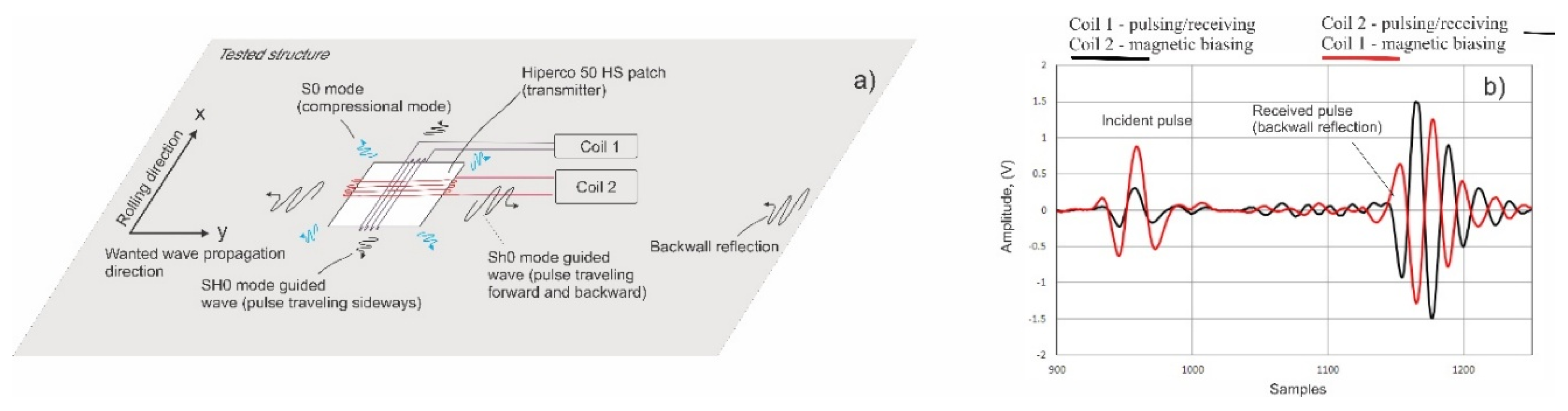
Figure 2.
Results of vibration readings from a 304 x 304 mm aluminum plate with an SH0 mode probe coupled to one side of the plate: a – experiment arrangements, b - Wanted SH0 mode accompanied by unwanted S0 mode; c - SH0 modes going sideways and creating additional waves.
Figure 2.
Results of vibration readings from a 304 x 304 mm aluminum plate with an SH0 mode probe coupled to one side of the plate: a – experiment arrangements, b - Wanted SH0 mode accompanied by unwanted S0 mode; c - SH0 modes going sideways and creating additional waves.
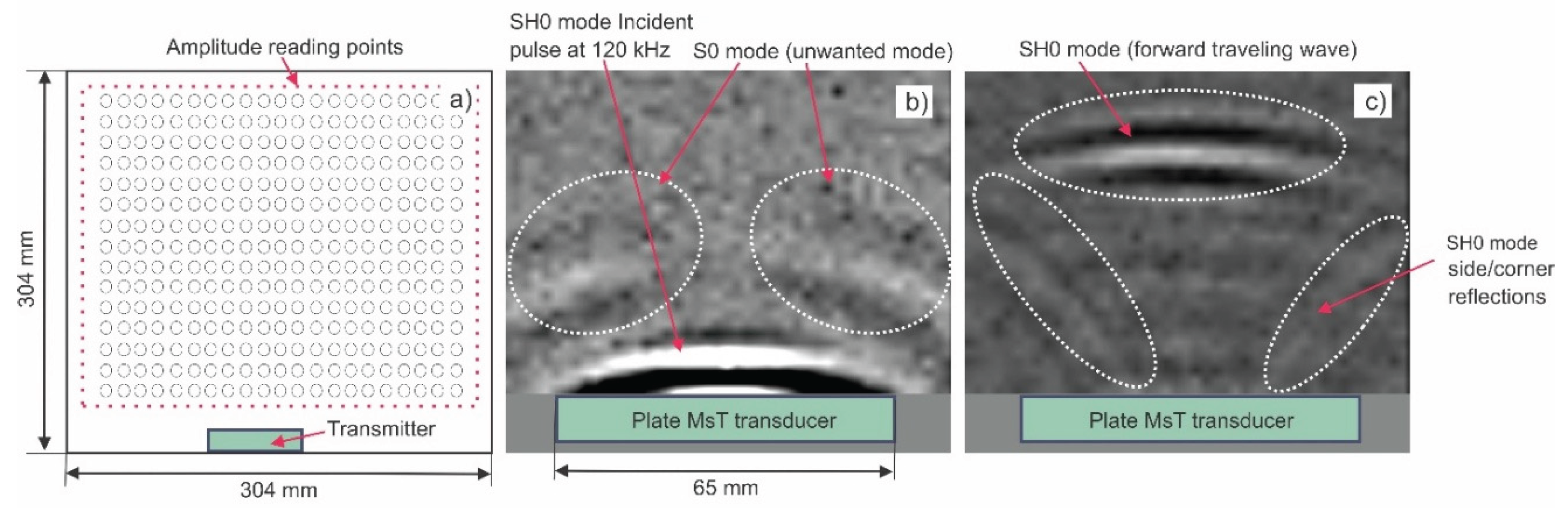
Figure 3.
Principal design of reversed Wiedemann effect MsT probe.
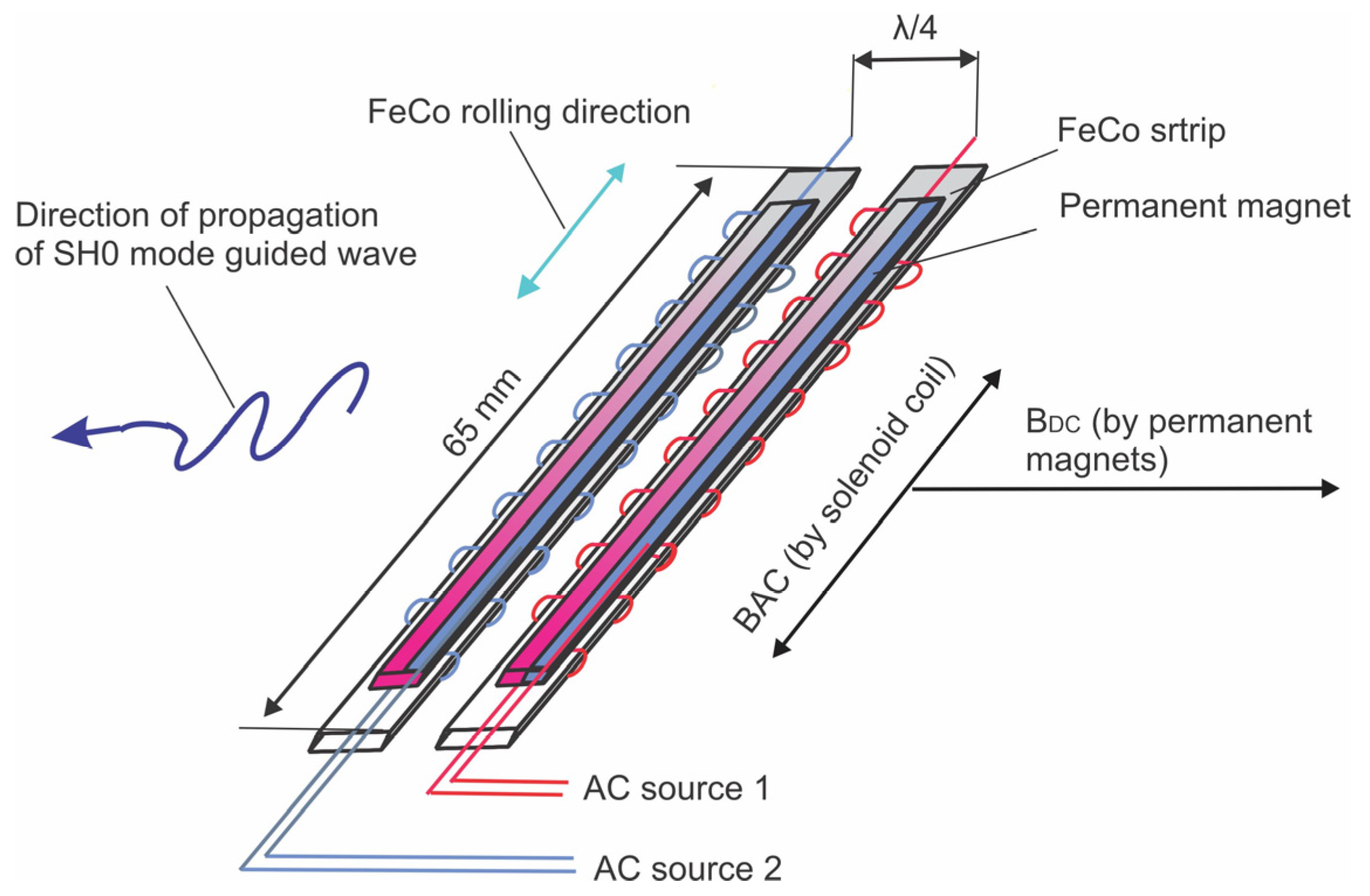
Figure 4.
Magnetostrictive array system: a- MsSRV5M instrument with MsT 8x8 array probe; b – 8x8 probe installed on a storage tank bottom extension; c – probe installed on wall of a large storage tank.
Figure 4.
Magnetostrictive array system: a- MsSRV5M instrument with MsT 8x8 array probe; b – 8x8 probe installed on a storage tank bottom extension; c – probe installed on wall of a large storage tank.
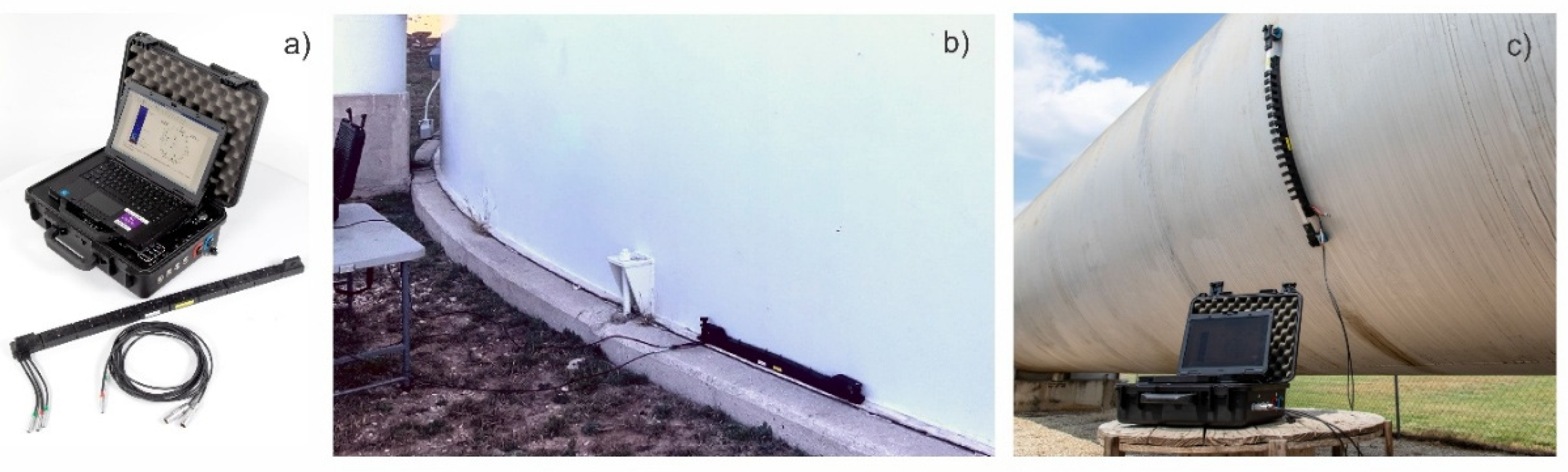
Figure 5.
Data acquisition protocols used with 8x8 array MsT probe: a – segments engaged when acquiring data for SAFT, CSM, and TFM algorithms; b – number of data sets collected for each algorithm when using 4x4 array probe and 8x8 array.
Figure 5.
Data acquisition protocols used with 8x8 array MsT probe: a – segments engaged when acquiring data for SAFT, CSM, and TFM algorithms; b – number of data sets collected for each algorithm when using 4x4 array probe and 8x8 array.
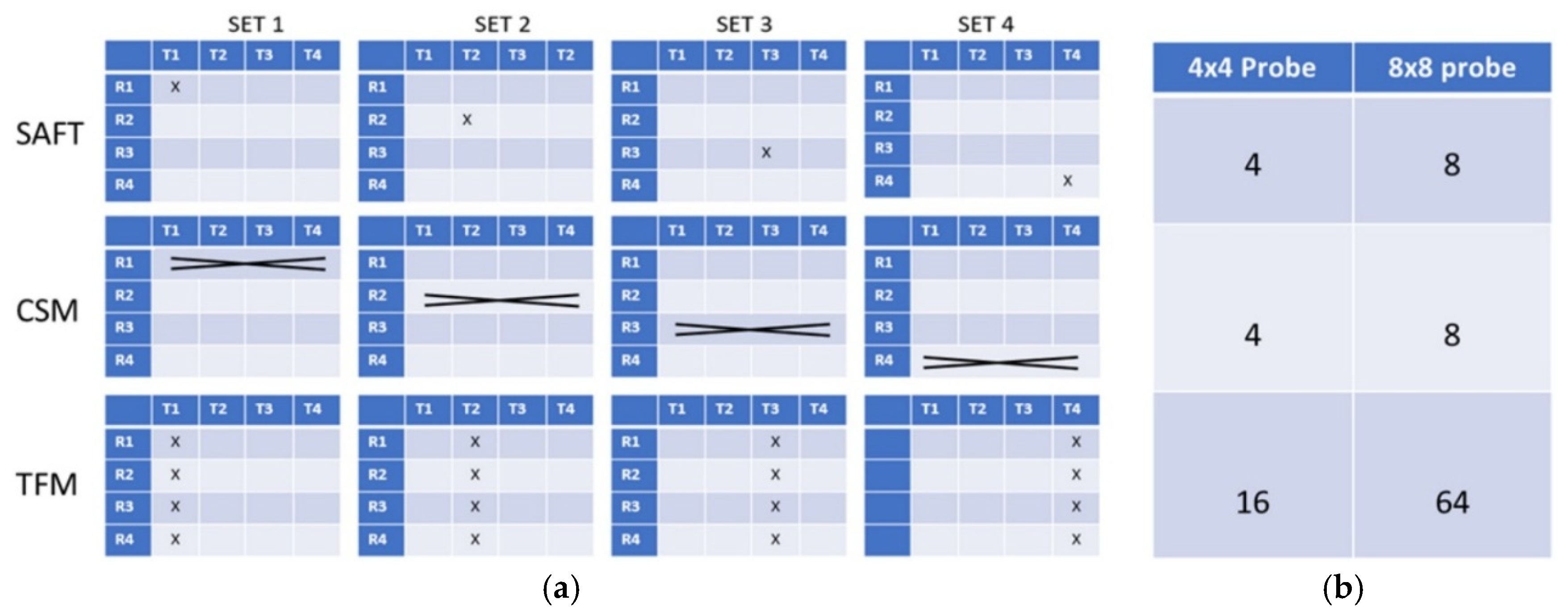
Figure 6.
Example of anomaly imaging in a mockup plate using these three methods at 180 kHz: a –TFM results over the full plate; b – TFM image of the area with notches; c – CSM image of the area with notches; d) – SAFT image of the area with notches.
Figure 6.
Example of anomaly imaging in a mockup plate using these three methods at 180 kHz: a –TFM results over the full plate; b – TFM image of the area with notches; c – CSM image of the area with notches; d) – SAFT image of the area with notches.
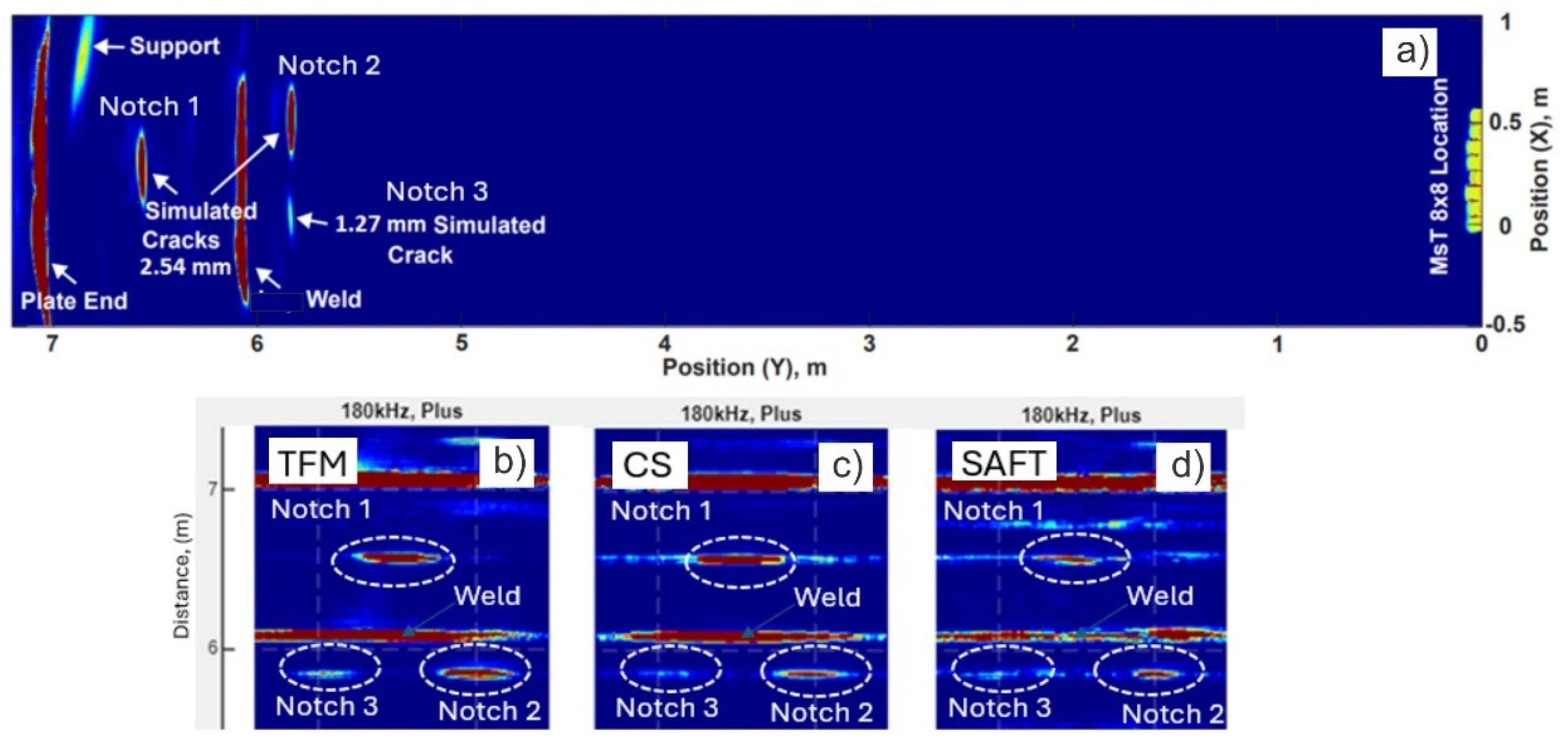
Figure 7.
TFM image in storage tank wall obtained at 30 kHz with the 8x8 probe mounted on tank bottom extension at zero distance mark.
Figure 7.
TFM image in storage tank wall obtained at 30 kHz with the 8x8 probe mounted on tank bottom extension at zero distance mark.
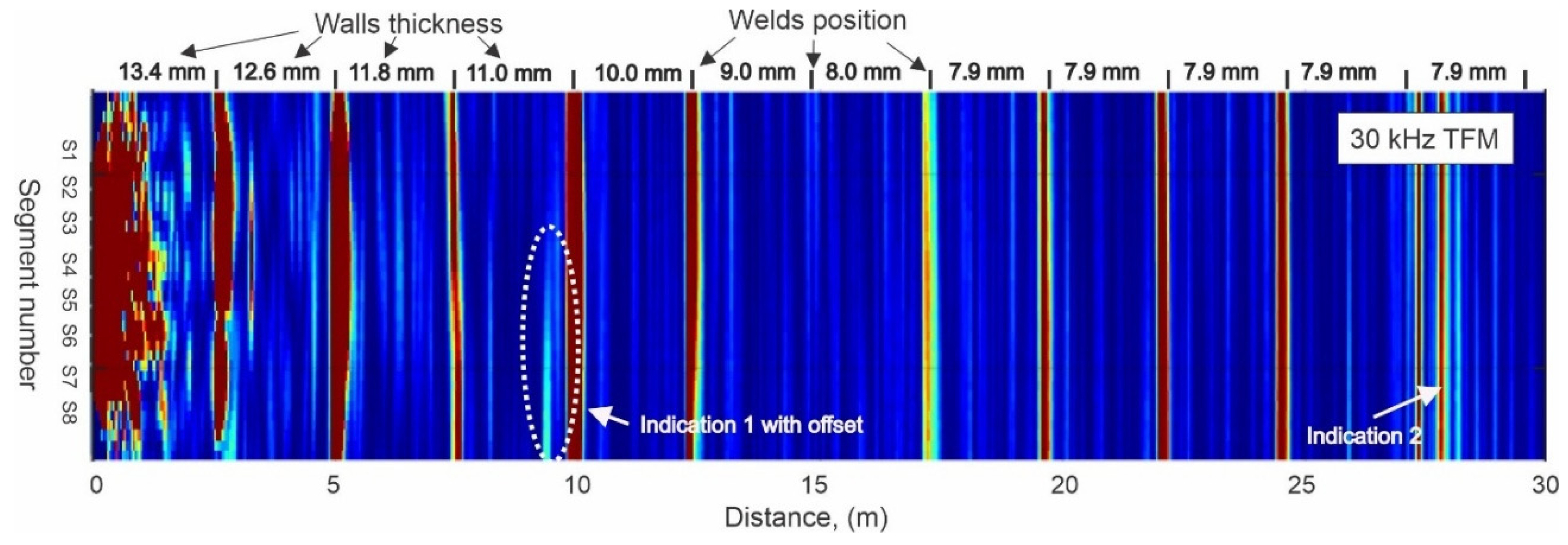
Figure 8.
Challenges of tank bottom inspection using guided waves: a – penetration of guided waves in the tank bottom as well as in the vertical wall; b – example of data acquired from 10 m diameter butt-welded tank bottom.
Figure 8.
Challenges of tank bottom inspection using guided waves: a – penetration of guided waves in the tank bottom as well as in the vertical wall; b – example of data acquired from 10 m diameter butt-welded tank bottom.
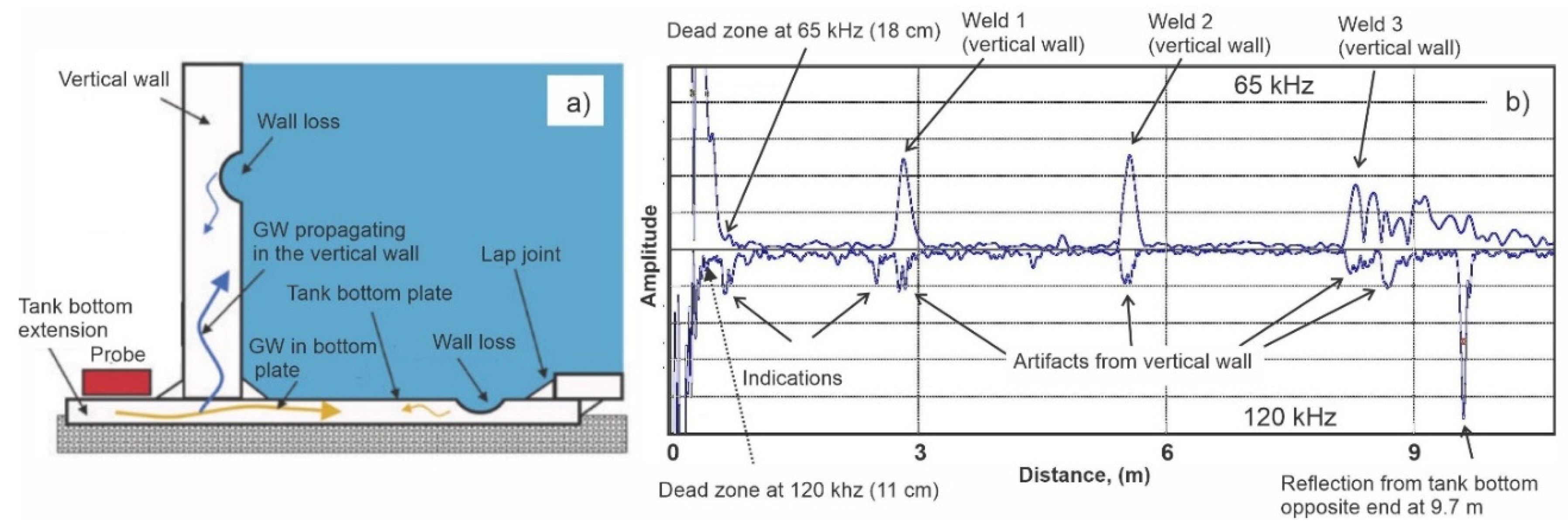
Figure 9.
Probe testing on 260x210x7 mm carbon steel plate: a- B-scan image obtained using 8 segment probe at 64 kHz; b – A scan using segment pair S1-S1; c – A scan using segment pair S1-S2; d – A scan using segment pair S1-S3; e – A scan using segment pair S1-S4.
Figure 9.
Probe testing on 260x210x7 mm carbon steel plate: a- B-scan image obtained using 8 segment probe at 64 kHz; b – A scan using segment pair S1-S1; c – A scan using segment pair S1-S2; d – A scan using segment pair S1-S3; e – A scan using segment pair S1-S4.
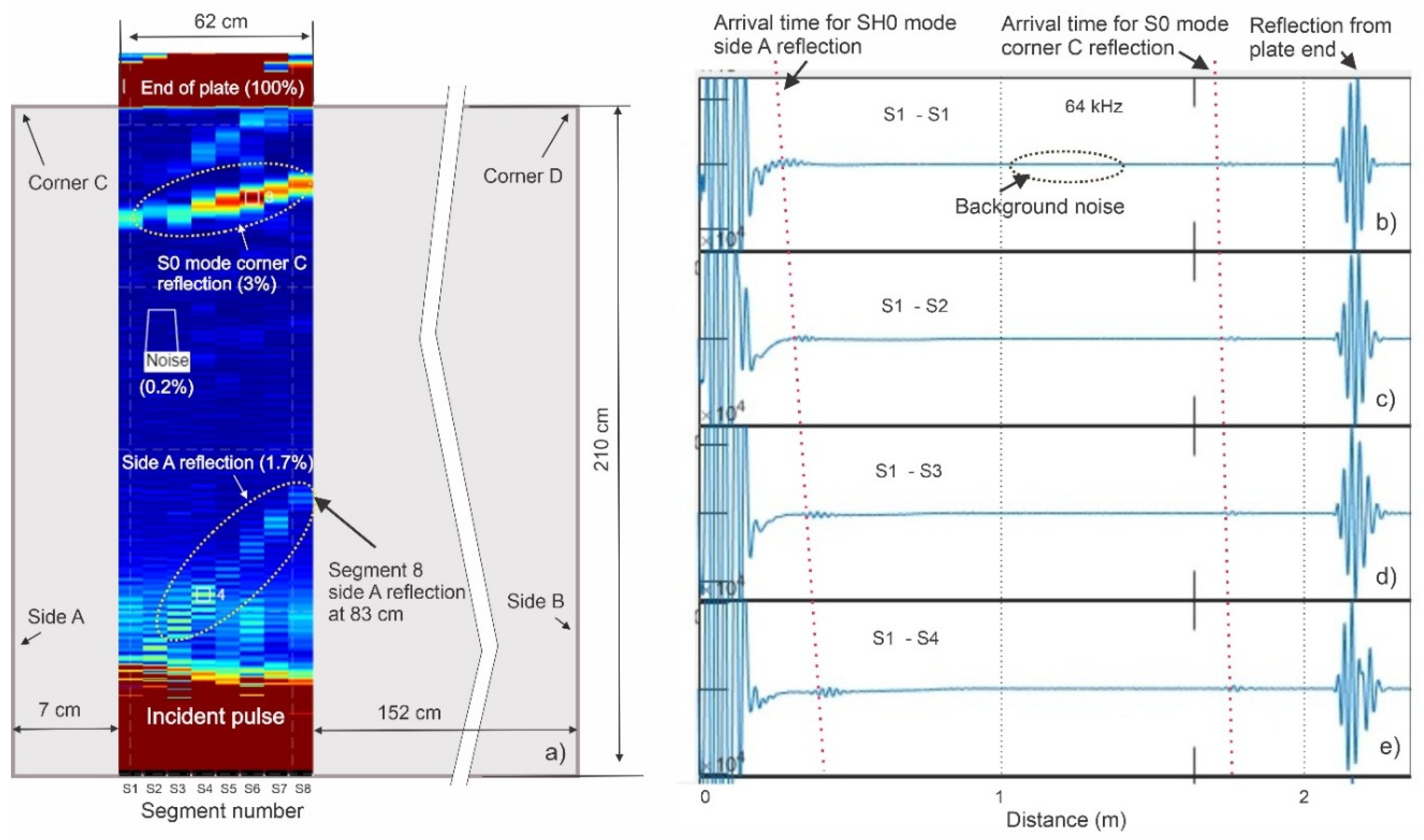
Figure 10.
Tank bottom mockup with a lap weld: a- internal view of mockup plate; b – external view of mockup plate showing position of the 8x8 probe.
Figure 10.
Tank bottom mockup with a lap weld: a- internal view of mockup plate; b – external view of mockup plate showing position of the 8x8 probe.
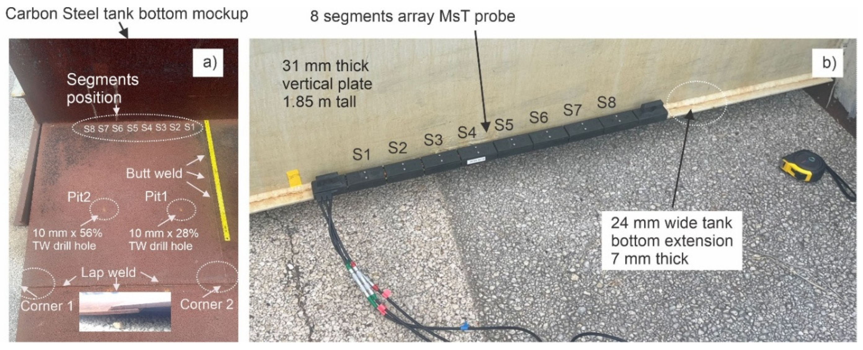
Figure 11.
Indication reports from tank bottom mockup at 90 kHz: a - 8x8 B-scan plot; b - 8x8 SAFT plot, c - 8x8 TFM plot, d - 4x4 TFM plot using segments 1 – 4, e - 4x4 TFM plot using segments 5 – 8.
Figure 11.
Indication reports from tank bottom mockup at 90 kHz: a - 8x8 B-scan plot; b - 8x8 SAFT plot, c - 8x8 TFM plot, d - 4x4 TFM plot using segments 1 – 4, e - 4x4 TFM plot using segments 5 – 8.
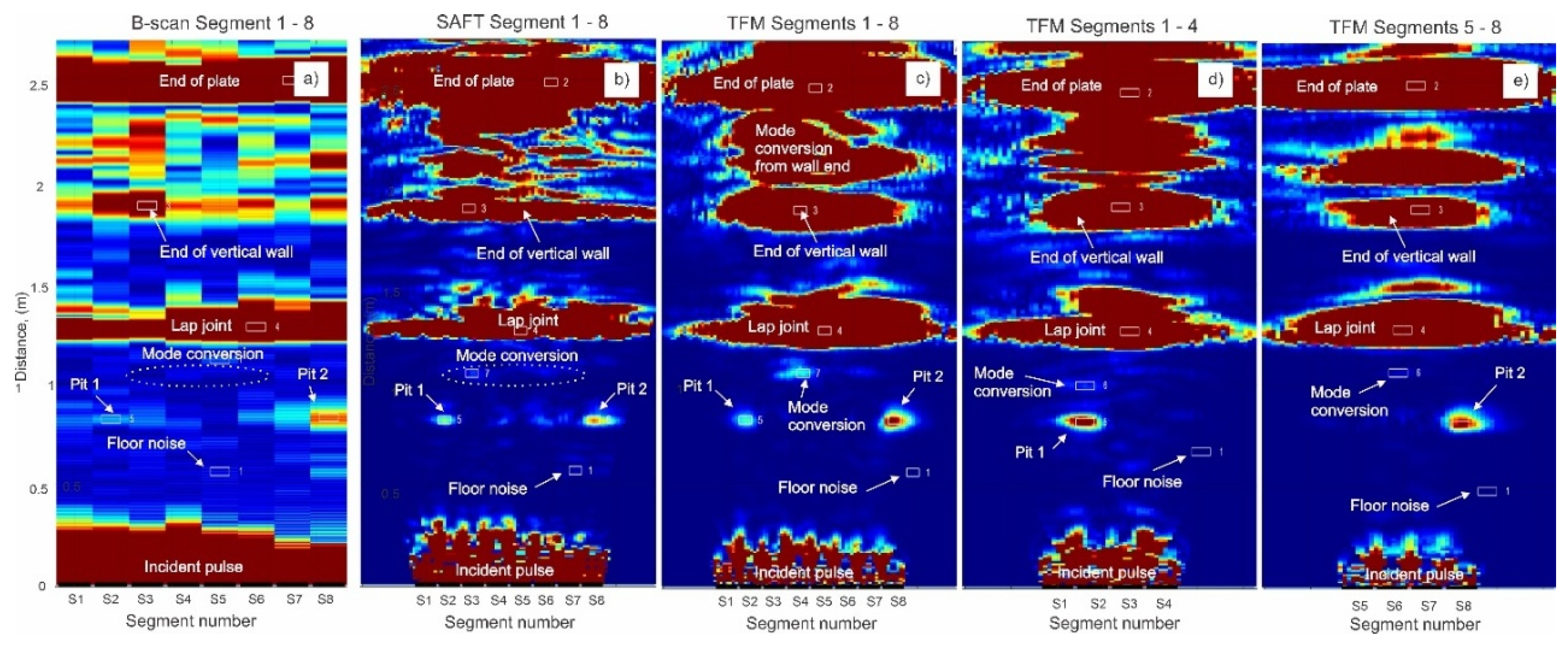
Figure 12.
SNR for each indication shown in Figure 11.
Figure 12.
SNR for each indication shown in Figure 11.
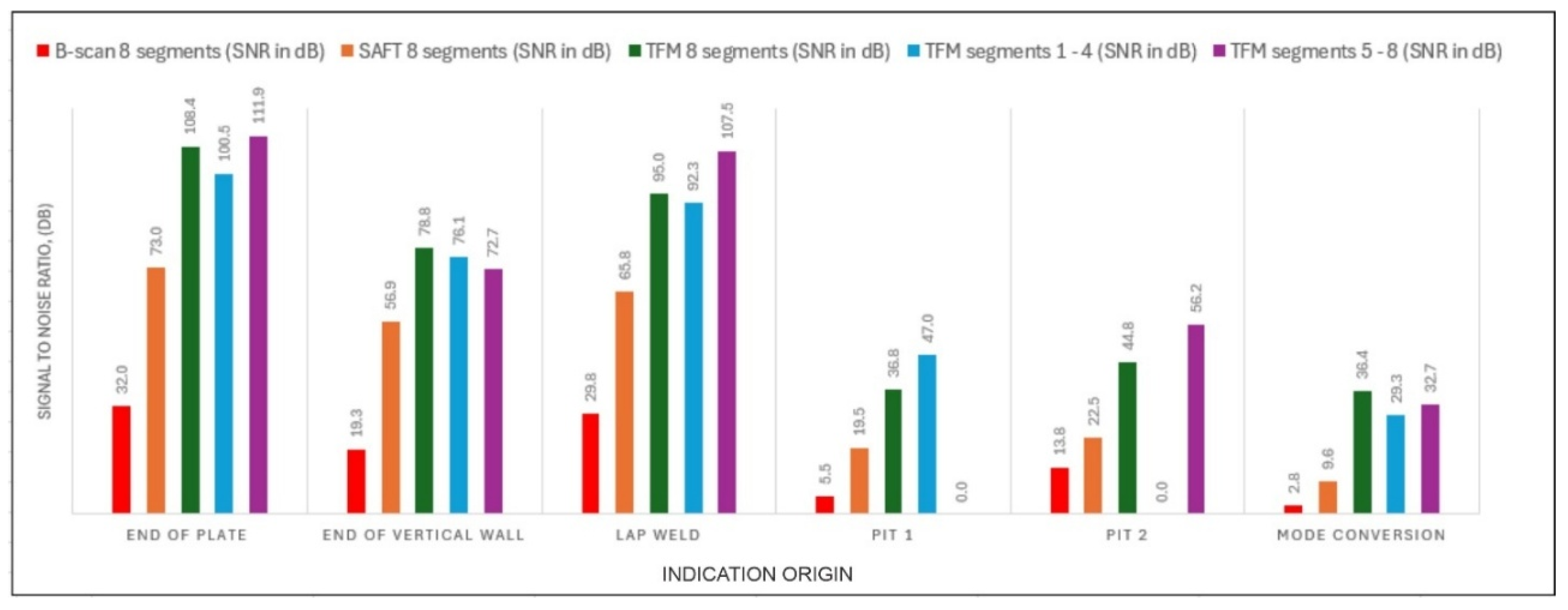
Figure 13.
GW testing of storage tank: a – lap welded bottom geometry and probe position; b – TFM plot at 64 kHz, c – TFM plot at45 kHz, d – TFM plot at 32 kHz. .
Figure 13.
GW testing of storage tank: a – lap welded bottom geometry and probe position; b – TFM plot at 64 kHz, c – TFM plot at45 kHz, d – TFM plot at 32 kHz. .
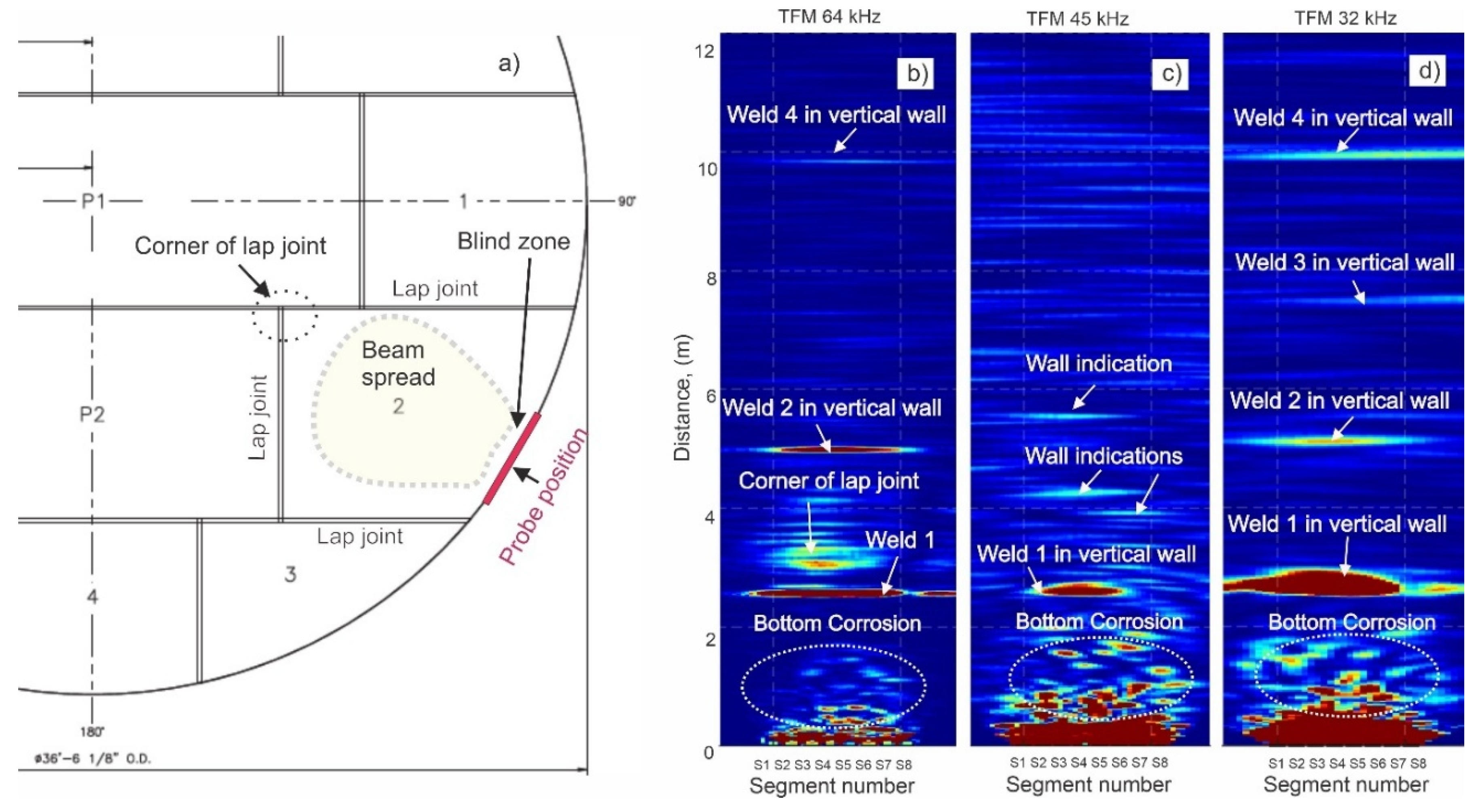
Figure 14.
Results of anomaly ranking in tank bottom at 64 kHz : a – TFM plot showing the reference weld and area with suspect indications; b – a list of indications with relevant amplitude and position information. .
Figure 14.
Results of anomaly ranking in tank bottom at 64 kHz : a – TFM plot showing the reference weld and area with suspect indications; b – a list of indications with relevant amplitude and position information. .
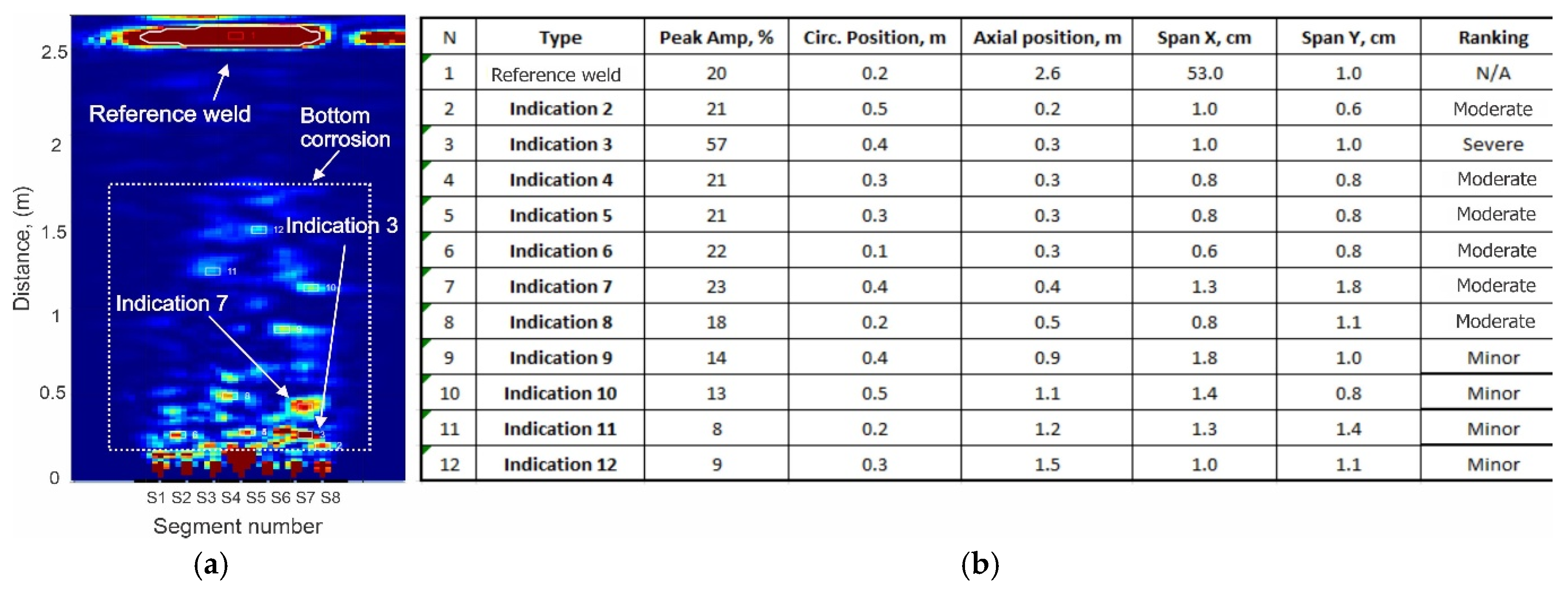

Table 1.
Accomplished SNR values for indications shown on Figure 11.
Table 1.
Accomplished SNR values for indications shown on Figure 11.
 |
Disclaimer/Publisher’s Note: The statements, opinions and data contained in all publications are solely those of the individual author(s) and contributor(s) and not of MDPI and/or the editor(s). MDPI and/or the editor(s) disclaim responsibility for any injury to people or property resulting from any ideas, methods, instructions or products referred to in the content. |
© 2026 by the authors. Licensee MDPI, Basel, Switzerland. This article is an open access article distributed under the terms and conditions of the Creative Commons Attribution (CC BY) license.
Copyright: This open access article is published under a Creative Commons CC BY 4.0 license, which permit the free download, distribution, and reuse, provided that the author and preprint are cited in any reuse.


