
Submitted:
08 January 2026
Posted:
09 January 2026
You are already at the latest version
Abstract
This study constructs a global timber trade network (2004-2023) to model underload cascading failures, assessing node-level disruptiveness and resilience. The network has grown structurally integrated, with density rising and path length shortening. Export-oriented economies (e.g., Canada, Vietnam) prove more susceptible to cascading failures than import-oriented ones (e.g., China, Japan), confirming upstream-to-downstream failure propagation. Node disruptiveness is heterogeneous: major exporters (Canada, Germany) cause the largest efficiency losses, while intermediaries (South Africa) impair connectivity. Out-strength and betweenness centrality are key determinants of disruptiveness. Resilience in 2023 varies widely; China's diversified sourcing enhances its resilience, whereas the U.S., Japan, and South Korea face higher vulnerability due to supply concentration. Overall, declining resilience among major importers underscores growing systemic risks. Although strategic diversification improves individual positions, large-scale disruptions remain a considerable threat, highlighting the imperative for optimized sourcing and robust contingency planning to stabilize global timber flows.
Keywords:
the global timber trade network
; node disruptiveness
; node resilience
; underload cascading failure
; complex network
1. Introduction
1.1. Research Background
As timber is a strategic resource with economic, ecological, and renewable value [1], its supply stability directly influences national resource security and regional economic stability [1]. In 2022, wood product exports reached a record high of $576 billion [2]. Forest resources are unevenly distributed globally [3], predominantly located in countries such as Russia, Brazil, Canada, and the United States [4]. Many countries rely on timber trade to balance supply and demand, promote economic development, and address market demands. The timber trade constitutes a transnational complex network, whose structure and dynamics have drawn increasing scholarly interest. Against the backdrop of intensifying global resource competition, timber supply has transcended conventional economic dimensions to emerge as a strategic resource security issue. [6]. Environmental protection, resource endowments, and geopolitical factors contribute to an increased risk of disruptions in timber-supplying countries. Disruptions may trigger cascading failures, resulting in substantial damage to the Global Timber Trade Network (GTTN) and potentially culminating in network collapse. Scientific models are needed to elucidate disruption propagation mechanisms and evaluate both node disruptiveness and node resilience within the network. This enables the identification of vulnerable segments and potential risks under internal and external shocks. Therefore, research on node disruptiveness and node resilience in the timber trade network is essential for identifying critical nodes, safeguarding timber resource security, and supporting stable global economic development.
1.2. Current Research Status of Forest Product Trade Networks
Complex network modeling and simulation have been widely applied by scholars to study the international timber trade network in depth. Tian and Jiang (2016) [5] were the first to identify core countries in the international log trade network during 2005–2014, highlighting the significant impact of economic conditions and government policies on trade. He (2018) [6] applied complex network theory to analyze the global timber supply network over a longer period (2001–2016), revealing clustering characteristics and an increasing role of China in global timber trade. Wang et al. (2021) [7] developed a directed weighted network model of forest product trade using longitudinal data (1993-2018), revealing China, the Netherlands, France and the United States as structural hubs in the global timber trade system. Zhou et al. (2021) [8] investigated the evolution of the global log trade network from 2000 to 2018, observing a tendency for core countries to form clusters, with China’s centrality continuously rising. Tian et al. (2022) [9] examined the competitive and complementary aspects of timber product trade between China and ASEAN, noting an increase in trade network density while competitiveness intensified. Li et al. (2022) [10] analyzed the structure and influencing factors of timber product trade networks among RCEP member countries, highlighting China’s central position. Wang et al. (2023) [11] analyzed global forest product trade data from 2000 to 2020 and found that the trade network of processed forest products has become increasingly interconnected, with high-income economies holding a dominant position within the network. Liu et al. (2024) [12] conducted a comprehensive analysis of the global timber forest product trade network covering data from 1995 to 2020, indicating that North America, Europe, and developing countries in Asia have become core regions. Gao (2024) [12] explored changes in complexity and centrality within timber product trade networks, suggesting that free trade agreements intensify the uneven distribution of global forest resources. Liu et al. (2024) [13] measured and compared the resilience of forest product trade networks under static and dynamic conditions, simulating the effects of random and targeted attacks. Research indicates that downstream forest product trade networks exhibit greater resilience compared to upstream networks, and structural optimization can significantly enhance the stability of the global forest product trade system.
Studies have shown that the global forest product trade network exhibits significant scale-free and small-world properties. With the deepening of trade relationships and expansion of scale, the network structure becomes increasingly ordered, and bidirectional exchanges between countries are enhanced. These findings not only reveal the complexity of trade networks but also provide important references for China’s participation in global trade. However, most existing studies neglect the weighted nature of supply paths, resulting in insufficient consideration of weights in key network metrics such as average path length and Global Efficiency Loss Rate, thereby limiting the practical value of the models. To address this limitation, a weighted forest product trade network modeling method based on supply-demand closeness was proposed by our research team (2024) [13], offering a new perspective for related research.
1.3. Current Research Status of Networks Resilience
Trade network research is shifting from structural analysis to resilience assessment to address resource supply security challenges under globalization. Network resilience has become a core topic for ensuring system stability, but it remains at an early stage of exploration. Existing studies include: multi-layer models were applied by Caschili et al. (2015) [14] to analyze and simulate the resilience of international trade systems, providing new perspectives on understanding global trade network resilience. Yuan et al. (2022) [15] studied the global crude oil trade network from 2007 to 2020 and found that the network expanded and became more tightly connected, with core countries exerting significant influence on resilience. Ji et al. (2024) [13] investigated the dynamics and Node Vulnerability of global trade networks for four major food crops from 2000 to 2019. Simulations indicated that disruptions in 5% of countries could severely impair network stability, highlighting the importance of identifying critical nodes and enhancing resilience strategies. Chen et al. (2023) [16] analyzed the global phosphorus trade network from 1990 to 2020 and found an average resilience of 0.24, characterized by high redundancy but low efficiency, with trade fluctuations of core countries having significant impacts, while path diversity helped mitigate shocks. Yu et al. (2024) [17] studied the global supply networks of gallium, germanium, and silicon from 2013 to 2022 and found that gallium and germanium networks showed improved structural resilience but increased vulnerability, whereas the silicon network exhibited the opposite trend. Resilience measurement studies on international energy trade networks were conducted by Jiao. (2024) [18] from an energy security perspective, revealing that core node countries are crucial for network stability, and suggesting that policy coordination and technological innovation can enhance overall resilience. Zhou et al. (2024) [19] examined rare earth supply networks, particularly the application of neodymium-iron-boron permanent magnets, finding that despite the complexity and diversity of the global supply chain, China still dominates, indicating the need for strengthened international cooperation to ensure resource security. Zhong et al. (2024) [17] investigated the resilience of crude oil maritime supply chain networks under uncertain disturbances and found that establishing flexible transportation routes and reserve mechanisms are effective means to cope with uncertainties. Chen et al. (2024) [17] analyzed the trade network structure and resilience along the Belt and Road Initiative regions and found that inter-regional trade connections have become increasingly tight but continue to face multiple challenges such as geopolitical risks, requiring enhanced connectivity to promote shared prosperity. Zuo et al. (2024) [17]studied the trade patterns and Node Vulnerability of the global lithium industry chain and found that uneven distribution of lithium ore resources intensifies market volatility, necessitating diversified supply sources to improve resilience. Shen et al. (2024) [17] investigated Node Resilience in critical mineral supply chain networks under sudden risks and revealed that bottleneck nodes are particularly vulnerable during emergencies, proposing optimized node layouts to enhance overall risk resistance. Current research focuses on the relationship between trade network resilience, structural characteristics, and types of attacks, but the indicators remain scattered, and risk propagation mechanisms under disturbance failures have not been thoroughly explored.
The dynamic response mechanism of resource trade networks after external disruptions is a central aspect in understanding system resilience. The study by Li Yingli (2024) [17] did not directly investigate the resilience mechanism of the cobalt supply chain, but the analysis of its “robust yet fragile” characteristic provided meaningful insights. A systematic framework for network resilience assessment has not been established in academia. Future research on resource networks should prioritize two key dimensions: first, the analysis of dynamic response mechanisms following disruptions; second, the development of dedicated methods for resilience assessment. This research direction is expected to advance theoretical understanding and support improvements in network risk resistance.
1.4. Current Research Status of Cascading Failures
Cascading Failures represent a key mechanism in network resilience research, describing a chain reaction process in which node failures induce load redistribution and thereby cause subsequent failures of adjacent nodes [20]. The mechanism has a significant impact on the overall stability and reliability of systems.
Existing models of Cascading Failures include the Load-Capacity model, CASCADE model, Sandpile model, Optimal Power Flow model, and Binary Influence model. The Load-Capacity model simulates cascading failures caused by dynamic load redistribution through defined initial node loads and capacity thresholds. For instance, Wang et al. (2023) [21] reported that expanding core nodes in the bauxite trade network could reduce cascading failure size by 42%. The CASCADE model focuses on continuous avalanche effects. Sun et al. (2022) [21] applied this model to quantify an indirect propagation contribution rate of 45% in cobalt trade, while Zheng et al. (2022) [21] combined it with the Sandpile model to show that Russian sanctions resulted in an 18% efficiency loss in European energy control transfer. The Sandpile model highlights system criticality characteristics. Yan et al. (2024) [21] demonstrated that oil network stability decreases exponentially with increasing complexity, and Lee and Goh (2016) [21] observed a 50% increase in overall failure probability due to collapse of weak layers in multi-layer trade networks. The Optimal Power Flow model is used to optimize resource allocation. Zhao et al. (2023) [21] showed that expanding core nodes in wind power networks reduces cascading failure size by 30%, while Craig et al. (2019) [21] achieved only a 2.1% revenue reduction under environmental constraints in small hydropower systems. The Binary Influence model triggers failures based on threshold values. Xiao et al. (2022) [21] confirmed that targeted attacks on photovoltaic trade networks cause collapse at 2.3 times the normal speed, and Cai and Song (2016) [21] revealed that collapse of core countries leads to an 80% break in peripheral trade. Furthermore, multi-model coupling expands application scenarios. Zhou et al. (2022) [21] simulated that China’s ban on waste rubber exports amplified cascading effects on US exports by 3.2 times. A summary of these cascading failure models and their comparisons in trade network analysis is presented in Table 1.

Table 1.
Comparison of Multiple Cascading Failure Research Models.
| Model types | Core mechanisms | Advantages | Limitations | Typical Scenarios |
|---|---|---|---|---|
| Load-Capacity model [22,23] | Failure is triggered when node load exceeds the capacity threshold, followed by cascading propagation due to load redistribution. | Provides intuitive reflection of overload impact, enables quantification of node tolerance. | Limited in capturing nonlinear effects (e.g., dynamic feedback). | Overload collapse in power grids, congestion propagation in logistics networks. |
| Sandpile model [24,25] | Node collapse occurs when load accumulates to a critical value, following the theory of self-organized criticality. | Describes chain collapse triggered by stochastic perturbations, reveals system phase transitions. | Difficult to accurately predict collapse thresholds, relies on simplified assumptions. | Traffic flow avalanches, cascading failures in power systems. |
| CASCADE model [26] | Node failure probability increases with the number of adjacent failed nodes, governed by probabilistic propagation rules. | Supports efficient dynamic simulation, applicable to large-scale network analysis. | Poorly adaptable to complex topologies (e.g., multi-layer heterogeneous networks). | Financial risk contagion, supply chain disruption diffusion. |
| Binary Influence model [27] | Node state is binary (intact/failed), and failure propagation is triggered by Boolean logic (e.g., proportion of failed neighbors exceeds a threshold). | Exhibits low computational complexity, suitable for fast propagation path simulation. | Neglects gradual node state changes and network dynamic weights. | Rumor spreading, trust chain breakdown. |
| Optimal Power Flow model [28] | Cascading failures are simulated based on power grid physical constraints (power balance, voltage stability), combined with engineering optimization methods. | Accurately represents physical layer constraints, supports resilience-cost trade-off analysis. | Application restricted to power systems, associated with high model complexity. | Power grid collapse simulation, electricity supply-demand imbalance risk prediction. |
The Load-Capacity model is the most commonly used model for studying Cascading Failures. The occurrence of cascading failures in this model mainly depends on three factors: initial load, load capacity, and load redistribution strategy [29,30]. Research on load-capacity-based cascading failures has attracted increasing attention in the field of resource trade networks. Li et al. (2021) [31] developed a cascading failure model to simulate the avalanche process in the global plastic waste trade network after fault events. Hao et al. (2023) [31] constructed the global lithium trade network and simulated its robustness under random and targeted disruption scenarios. Fu et al. (2024) [31] analyzed the resilience of automotive manufacturing supply chain networks against cascading failures and found that underloaded nodes after load redistribution significantly reduce network resilience. The attack strategy based on high eigenvector centrality was shown to cause the most severe damage. Yin et al. (2024) [31], through modeling and simulation, investigated the propagation mechanisms of cascading failures in the international semiconductor trade network. Wang et al. (2024) [31] studied risk propagation in the Global Iron Ore Trade Network (GTTN), modifying the cascading failure model to incorporate national-level risk absorption and adaptation capabilities. Ouyang et al. (2024) [31] identified systemic risks in the global lithium supply network, particularly its vulnerability to cascading failures, and emphasized the need for global cooperation to balance efficiency and security. Miao et al. (2024) [31] established a cascading failure model to explore internal mechanisms and supply risk propagation in the polycrystalline silicon trade network, demonstrating the critical role of core node countries in improving network stability and resilience. Despite the insights provided by these models, further research is needed to better understand the specific influencing factors and dynamic response characteristics across different network types.
Currently, research on Cascading Failures in complex networks has developed a relatively mature theoretical framework for overload-induced failures. In contrast, studies on Underload Cascading Failure under trade network disruptions remain at an early stage.
Based on previous studies on path-weighted static resilience and dynamic structural resilience, this work presents a systematic investigation of timber supply network resilience from three aspects: data classification, model improvement, and node resilience. The key innovations and contributions are summarized as follows. First, in data classification, wood and forest products are categorized in greater detail, with a focus on logs and sawn wood as two representative upstream timber types. Compared to earlier studies that grouped logs, sawn wood, and wood pulp into a single category, the proposed classification improves data completeness and comparability, supports standardized analysis, and enables more precise identification of supply chain stability and disruption resistance mechanisms. Second, for model improvement, the Underload Cascading Failure model is modified to improve its applicability and simulation accuracy within the Global Timber Trade Network (GTTN), thereby better representing shock propagation processes and providing a solid foundation for resilience assessment. Third, regarding node resilience, a metric system based on time-cumulative effects is developed to quantify node resilience, capturing the ability of nodes to maintain performance or function under continuous disruptions. Given the decentralized structure of the Global Timber Trade Network, where individual countries act as critical nodes, the study of node resilience is practically significant. This metric overcomes the limitations of traditional instantaneous indicators in characterizing long-term node behavior, offering a new perspective on the dynamic response mechanisms of trade networks.
2. Data Sources and Analytical Framework
2.1. Data Acquisition and Research Framework
This study focuses on logs and sawn wood, including fuelwood, wood chips, and other primary processed products, excluding bamboo, rattan, and straw. The selection is based on three considerations. First, logs and sawn wood are key products in the global timber trade network (GTTN), and their trade patterns directly reflect supply stability and node resilience. Second, international trade data for these products are well standardized, ensuring data reliability. Finally, they best represent the supply stability of raw materials and the resilience characteristics of the network. Based on this scope, relevant data were collected according to the HS codes defined by the World Customs Organization, as shown in Table 2.
The HS coding system offers advantages such as high standardization, broad coverage, and low data acquisition costs. However, it also has limitations, including statistical discrepancies across countries, data missingness, and delays in updates. To address these issues, future research could integrate supply chain data, satellite remote sensing, and industry statistics to build a multi-source data fusion analytical framework. Based on the HS coding system, this study uses import trade data to ensure consistency and comparability. The data were obtained from the UN Comtrade database, covering timber trade flows among 231 countries (regions) globally from 2004 to 2023, with over 500,000 valid import records integrated. Trade volume (kg) is applied as edge weight to eliminate the influence of price fluctuations, directly reflecting inter-country supply dependencies and objectively characterizing supply-demand structure and network resilience features.
Missing trade volume data are addressed using a hierarchical mean imputation method. Missing values are filled with the mean of non-missing records within groups defined by HS codes and years, ensuring temporal consistency and intra-group homogeneity. Noise data, identified by trade values below 50 USD, are removed to optimize network representation efficiency. Post-processing, total data volume decreases by 1%, network density increases by 2%, and efficiency indicators rise by 3%. Total trade volume declines by only 0.01%. These results indicate that the method effectively removes redundant connections and strengthens core dependencies.
Based on this, the study analyzes network performance loss and node performance loss under disruption propagation scenarios. An Underload Cascading Failure model and dynamic Node Resilience assessment indicators are constructed for this purpose. The analysis evaluates Node Disruptiveness, Node Dynamic Resilience, and their temporal evolution characteristics. Figure 1 delineates the comprehensive methodological structure. A spatiotemporal dual analysis framework is employed: spatially, a complex network of the GTTN, covering 231 countries and regions, is constructed; temporally, a dynamic evolution analysis model is established based on trade data from 2004 to 2023 spanning 20 years.
2.2. Construction of the Graph Theory Model
By treating countries (or regions) involved in the global timber trade as network nodes and their trade relationships as edges, with trade volume and trade proximity serving as weights, a complex network model is formulated. The Global Timber Trade Network (GTTN) is defined as follows:
Here, G represents GTTN; V denotes the set of all countries (regions); E denotes the set of trade relationships among all countries (regions); W¹ represents the set of trade volume weights between nodes; W² represents the set of trade cohesion weights between nodes; T represents the set of years.
This study employs a bilateral weight model, comprising trade volume edge weight and trade intensity edge weight. The trade intensity edge weight is derived from the trade relationship strength model previously proposed by the research team. The specific formula for computing this weight is as follows:
Here, represents the trade closeness between nodeand node; denotes the maximum trade volume of any edge in the network; and indicates the trade volume of timber exported from node to node . In reality, trade closeness may be influenced by various hard-to-quantify factors such as geopolitics, geographic proximity, and cultural differences. However, within the analytical framework of this study, the focus is solely on trade volume as the core factor.
2.3. Key Metrics of the Complex Network Model
The complex network-related indicators involved in this study are presented in Table 3.
2.4. Node Disruptiveness Assessment Metrics
Node disruptiveness quantifies the network performance degradation caused by node failures to identify critical nodes, providing a basis for network vulnerability assessment. This study employs the following two weighted performance metrics:
- (1)
- Weighted Global Efficiency Loss Rate
Weighted global efficiency loss rate quantifies the deterioration of overall network performance after stabilization of underload-induced cascading failures triggered by single-node disruptions, computed as:
Here, captures the post-disruption weighted global efficiency reduction when node i fails, represents the residual weighted global efficiency after the cascading failure triggered by the disruption of node i. denotes the baseline weighted global efficiency incorporating trade interdependence metrics.
- (2)
- Out-Strength Loss Rate in LCC
Out-strength loss rate in LCC is used as a key indicator to assess the integrity of the remaining network structure after supply disruptions. It measures the proportion of node out-strength loss in the largest connected component compared to its original out-strength. This ratio indicates how much core connectivity is preserved following disruption events. It serves as a fundamental basis for evaluating network resilience, connectivity preservation capability, and fault tolerance. The calculation formula for Out-Strength Loss Rate in LCC is as follows:
Out-trength loss rate in LCC quantifies the preservation degree of core connectivity after network disruptions, calculated as:
Here, represents the out-strength loss rate in LCC. is the total out-strength in the stabilized largest connected component (S’) after node i is removed. is the baseline total out-strength of nodes in the initial largest connected component (S) of the network.
2.5. Node Dynamic Resilience Assessment Metrics
Node Dynamic Resilience is quantified as the integral of the node performance retention ratio following sequential supply source disruptions. This method systematically characterizes node resilience under multiple supply failures. A constant time interval ∆t is assumed between consecutive node disruptions. Different disruption sequences correspond to permutations of the source node set . For a specific permutation:
Here, denotes the source node disruption sequence under the m-th simulation strategy, , and in is the in-degree of node . The performance of node after sequential disruption of the -th source node is represented by . Thus, the sequence describing node performance retention values is expressed as:
The sequence describing the node performance retention ratio is calculated as follows:
Of Which:
Here, denotes the start time of the disruption, and denotes the disruption time of node . Given the uncertainty in the node performance retention ratio curve, the segment between and is linearly approximated to simplify the calculation. The accumulated node performance retention over this interval is represented by the trapezoidal area under the curve from to. The corresponding formula is as follows:
To ensure comparability of resilience evaluation results across different nodes, a standardized disruption scale is adopted in this study: during simulations, a baseline scenario with k nodes disrupted is uniformly defined. This approach eliminates biases caused by variations in the number of supply source nodes among nodes, enabling comparison of those with distinct supply network topological features under identical disruption scales. As a result, the comparability of dynamic resilience metrics and validity of assessment outcomes are ensured. The dynamic resilience calculation formula for node after sequential disruption of k nodes is thus presented as follows:
Since the node performance retention ratio at time is equal to 1, Equation (10) can be further simplified as follows:
Further normalization of node dynamic resilience is achieved by dividing it by the initial retention value k×1. The calculation formula is as follows:
3. Construction of Disruption Risk Propagation Model
The underload cascading failure in the global timber trade network (GTTN) is fundamentally different from the overload cascading failure in infrastructure networks. Differences exist in failure triggering conditions, load distribution logic, and failure mitigation strategies, as detailed in Table 4.
This study utilizes a load-capacity model to simulate underload cascading failures in the GTTN, where supply node disruptions lead to downstream shortages. The model operates on a non-uniform redistribution logic, prioritizing high-weight edges to maintain their stability. It captures failure propagation along supply-demand paths (not physical topology) to identify critical nodes and vulnerable segments. The dynamic adjustment of export allocation also serves as a blocking strategy, providing actionable insights for preventing cascading failures and confirming the model’s suitability for GTTN risk analysis.
This study is based on the following assumptions:
(1) Supply-side dominance. Analysis focuses on supply-side disruptions (e.g., natural disasters, geopolitics), excluding demand and price mechanisms to clarify supply network structural responses.
(2) Structure-determined dynamics. Supply disruptions are treated as exogenous shocks, with their specific causes outside the scope of this study.
(3) Unidirectional cascading propagation. Disruption impacts propagate one-way from suppliers to receivers, without feedback effects from downstream to upstream nodes.
(4) Policy-mediated transmission. Disruption propagation is dominated by national-level policy interventions, surpassing market-based regulation at the firm level.
3.1. Model Core Parameters
The Underload Cascading Failure model defines a two-stage nodal response governed by two parameters: degradation capacity and failure capacity. Upon reaching the degradation capacity, a node enters the degradation stage and reduces exports adaptively. Exceeding the failure capacity triggers the failure stage, where exports cease entirely, potentially initiating multi-layer cascading failures. These capacities are set by the model’s initial load and thresholds.
Initial load defines a baseline state, enabling the model to reveal the network’s response patterns under disruption disturbances and evaluate its dynamic resilience. In the GTTN, initial load includes node-based and edge-based loads. The initial load of a node is defined by its import and export volumes, while the initial load of an edge is determined by the trade volume along that edge. The specific formulas are defined as follows:
Here, represents the initial import load of node i, corresponding to its in-strength before disruption. denotes the initial export load of node i, corresponding to its out-strength before disruption. indicates the initial load on the edge from node i to node j, corresponding to the trade volume weight of that edge before disruption.
This study improves the node threshold setting based on a previously developed Underload Cascading Failure model, integrating expert consultation and features of the GTTN. Based on grouped threshold settings, linear interpolation is applied within each group according to the import-export load ratios of nodes. This approach ensures that both degradation capacity and failure capacity retain inter-group differences while capturing the continuous distribution characteristics of nodes within groups.
(1)The ratio of node in-strength to node out-strength, denoted as θ, is calculated first. The formula for calculating for node is as follows:
(2) Nodes are grouped based on values, with maximum and minimum thresholds assigned to each group. Linear interpolation is performed within each group according to , where higher values correspond to higher thresholds. Considering practical conditions, nodes are classified into three groups, and the corresponding parameter settings are presented in Table 5. For simulation comparison purposes, two parameter sets are defined for each group: one for Strong Cascading Failure and one for Weak Cascading Failure.
In Table 5, for export-dominant nodes, a constant threshold setting scheme is applied. The failure threshold is set to 0, as these nodes are inherently insensitive to import underload, thereby preventing functional collapse during simulations. Given the significant difference in import-export load magnitudes, the degradation threshold is assigned a small constant value to represent the limited impact of import underload on such nodes. This method avoids unnecessary linear interpolation, conforms to the characteristics of the trade network, and enhances model computational efficiency.
The degradation capacity and failure capacity of the model are determined by the following formulas:
Here, denotes the decay capacity of node i, representing the maximum load reduction it can tolerate before entering the degradation stage. indicates the failure capacity of node i, reflecting the minimum load threshold below which the node becomes nonfunctional. The parameter denotes the decay threshold, controlling the decay capacity in simulations, while represents the failure threshold that defines the failure capacity.
3.2. Export Load Decay Function
The degradation function governs node out-strength adjustment under reduced import load. Dynamically derived from nodal trade characteristics and network performance requirements, it determines necessary out-strength reductions based on real-time node load and network state. According to the node classification in Table 5, distinct functions are defined for import-dominant, balanced, and export-dominant nodes (Table 6), ensuring accurate behavioral representation.
3.3. Redistribution of Export Loads
In the underload cascading failure model of the global timber trade network (GTTN), the export degradation allocation follows two principles: downstream node importance is determined by integrating local supply intensity with global topological influence; degradation is inversely allocated according to relationship strength, preferentially reducing weak-connection exports to maintain core link stability.
To implement this approach, the importance of trade relationships between downstream nodes is defined by the following formula:
Here, the importance of trade relationships is determined by the product of the trade volume between nodes and the eigenvector centrality of downstream node j, being proportional to both factors.
The outward-connected nodes of vertex i are sorted in increasing order of values to generate an ordered set , withdenoting the output connectivity degree of node i. The remaining distributable attenuation quantity is determined through the following computation:
Here, represents the residual distributable attenuation quantity for vertex i’s connection to adjacent node, while indicates the attenuation quantity assigned to this specific edge.
The cyclic allocation process at iteration t (initialized with ) follows:
Step 1: Neighbor-specific attenuation assignment
If >, compare with . If the former is larger, set ,otherwise, . If ,compare with , Assign accordingly.
Step 2: Residual quantity propagation
Update allocatable attenuation for subsequent neighbors:
Step 3: Iterative edge processing
Repeat Steps 1-2 until complete traversal of node i’s export connections.
The load redistribution modifies adjacent nodal loads, initiating iterative cascades until underload failure propagation stabilizes::
(a) Export load update:
(b) Global import load recalculation:
4. Results Analysis
4.1. Analysis of Overall Network Characteristics
From 2004 to 2023, the GTTN underwent significant structural streamlining: node count decreased from 214 to 205, while edges increased from 5,344 to 5,880 (Appendix A2), reflecting a shift towards a pruned yet more interconnected network. Sharp reductions in 2009 and 2020 marked the delayed impact of the 2008 financial crisis and the immediate shock of the COVID-19 pandemic, respectively. Concurrently, network density rose from 0.117 to 0.141, and average path length dropped from 1.957 to 1.935 (Appendix A3, unweighted & undirected), collectively enhancing transmission efficiency, resource allocation, and overall network resilience.
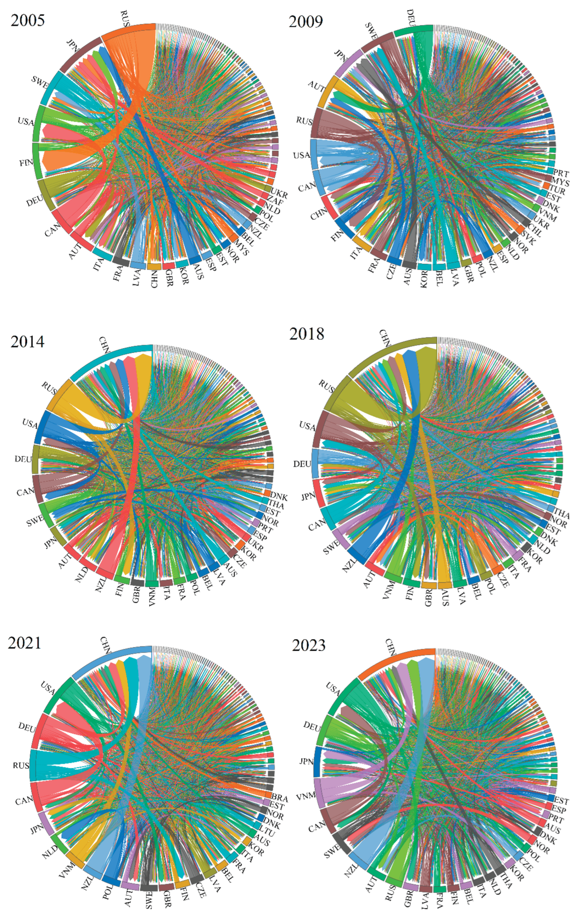
To clearly visualize the structural evolution of the GTTN, chord diagrams illustrate the network topology in 2005, 2009, 2014, 2018, 2021, and 2023 (Appendix A4). Arc width represents national/regional supply volume, and arrows indicate supply direction. These six snapshots reveal distinct timber trade patterns across countries.
Appendix A4 shows a resource-driven global timber supply pattern in 2005. Resource-rich nations (Russia, Canada) and industrialized countries (Japan, Germany) formed a core supply group, accounting for one-third of global supply. Russia, with its vast Far East coniferous forests, became the largest log exporter, contributing 22% of global exports, while Japan stood as a major importer. Regional supply clusters were clearly defined.
By 2009, the global supply structure shifted significantly: improved EU logistics and stable demand strengthened Germany and Austria as regional export hubs; Russia’s exports declined sharply due to log export tariff hikes (6.5% to 25%) and financial crisis impacts; and China’s RMB 4 trillion stimulus drove a 53% surge in timber imports, collectively reshaping global supply patterns.
In 2014, China became the world’s largest timber importer, driving Russia to resume its position as the top exporter. This shift was propelled by China’s urbanization (1.2 billion m² of new housing annually) and a 15% drop in domestic timber output due to forest conservation policies. Meanwhile, China–Russia tariffs fell from 15% to 5%, customs efficiency improved eightfold, and bilateral strategies aligned. As a result, China’s timber imports surged 96%, with Russian dependency reaching 61%.
By 2018, Russia remained the key supplier. Japan’s import growth was spurred by infrastructure projects for the Tokyo 2020 Olympics, while New Zealand entered a peak harvest period and Vietnam’s wood processing sector expanded rapidly, boosting both countries’ exports.
In 2021, Russia’s exports dropped sharply due to an early log export ban and major tariff hikes. Vietnam filled the gap through industrial upgrades, and New Zealand emerged as a core supplier with mature plantation resources.
In 2023, Russia’s exports further declined under the full log export ban and European sanctions. Benefiting from RCEP, Vietnam increased log and sawn timber exports to China, filling Europe’s supply gap and reflecting GTTN’s restructuring under geopolitical influences.
In summary, the evolution of the GTTN shows a three-stage pattern. The “resource–demand” dual structure (2005–2014) was initially shaped by Russia’s log export dominance and China’s demand. The policy-driven phase (2014–2021) then saw Russia’s export bans catalyze value chain upgrading, with Vietnam and New Zealand rising. Finally, post-2021, geopolitical forces solidified a new dual-loop structure of intra-Asia-Pacific and transatlantic trade, marking a shift from resource dominance to a geopolitics-and-efficiency dual-driver model.
4.2. Validation of Underload Cascading Failure Model
Using Python 3.12.3, single-node disruption simulations on 2023 GTTN key nodes validated the model and analyzed under-load cascading failures. Three parameter settings: No Cascading Failure, Weak Cascading Failure (Conservative Threshold), and Strong Cascading Failure (Sensitive Threshold). No Cascading Failure considered direct impacts only. Global Efficiency Loss Rate and Out-Strength Loss Rate in LCC were compared (Figure 2 and Figure 3). The cascade loss amplification factor (right axis) is the ratio of global efficiency loss rates between strong and no-cascading-failure scenarios.
Figure 2 and Figure 3 present results with countries ordered along the horizontal axis by their out-strength from low to high. Simulation results show that the amplification effect of export-oriented national cascading failures is significantly higher than that of import-oriented nations. The theoretical assumption that “Cascading Failures are triggered only by supply node disruptions propagating from upstream to downstream” is supported, confirming the model’s correctness. Additionally, loss rates caused by each node disruption follow strictly: Strong Cascading Failure > Weak Cascading Failure > No Cascading Failure. For instance, regarding Global Efficiency Loss Rate, the impact of Strong Cascading Failure in Canada is 17.68 times that of No Cascading Failure, while Out-Strength Loss Rate in LCC is 4.33 times higher. In Vietnam, these figures are 5.21 and 2.07 times, respectively; in Norway, they are 5.11 and 3.66 times. These findings align with theoretical expectations of Cascading Failures and further validate the model’s capability to capture cascading propagation dynamics.
Simulations reveal GTTN’s cascading failure traits:
(1) Cascading loss amplification is disproportionate to node out-strength. The United States, despite having the highest out-strength, shows a lower Global Efficiency Loss (0.23) than Canada—only 71.88% of the latter’s value, even with Canada’s out-strength being 27.64% lower. This reveals that cascading failure impacts are heterogeneous, driven by the interplay of the failed node’s properties and its downstream local topology.
(2) High node disruptiveness does not cause significant cascading amplification. The initial loss from a node disruption does not correlate with subsequent amplification. For example, China, a key importer, has an LCC Out-Strength Loss Rate of 0.26. Yet, it triggers little cascading due to its limited export connections. Meanwhile, New Zealand, a core exporter, shows a loss rate of 0.07 under No Cascading Failure. Its amplification factor under Strong Cascading Failure is only 1.38, constrained by its local topology. Thus, disruptiveness depends on resource supply capacity, while cascading effects are tied to network topology.
(3) The most destructive disruptions combine high node strength with significant cascading amplification. A node’s impact is determined by this interaction. Nodes like Canada, Vietnam, and Germany, which have both traits, cause severe damage. In contrast, nodes with high strength but low amplification (e.g., New Zealand) have limited influence. Similarly, nodes with low strength but high amplification (e.g., the Netherlands and Ukraine) pose minor threats.
4.3. Propagation Analysis of Underload Cascading Failures
To highlight the amplification effect and propagation mechanism of cascading failures, this section analyzes the diffusion process under the Strong Cascading Failure scenario for key nodes with significant transmission effects. Based on 2023 GTTN simulation data, Table 7 lists the cascading impact scope of 20 critical nodes after single-node disruptions. The table includes node attribute characteristics and the numbers of failed nodes and degraded nodes induced by Underload Cascading Failure.
Table 7 shows that a single-node disruptions in Canada leads to failure in 22 nodes and degradation in 43 nodes, affecting 65 countries or regions. This demonstrates the largest impact intensity and scope. In the United States, single-node failure causes 17 nodes to fail and 49 nodes to degrade, impacting 66 countries or regions. Although Germany’s cascading failure intensity is not high, its single-node disruptions results in failure of 16 nodes and degradation of 40 nodes, indicating a broad impact. South Africa, with a low node strength of only 2.3 million tons, experiences failure in 6 nodes and degradation in 43 nodes after disruption. This suggests high import dependency among downstream nodes. New Zealand, as the world’s third-largest timber exporter in 2023, sees only 1 node failing and 37 nodes degrading due to its disruption. This indicates lower dependence from downstream nodes and minimal overall network impact. Further analysis focuses on the cascading failure propagation processes of key nodes with significant Underload Cascading Failure transmission effects, including Canada, the United States, and emerging exporters like Vietnam and New Zealand.
The Underload Cascading Failure caused by Canada’s disruption is the single-node interruption with the largest impact intensity and scope. Figure 4 shows the propagation map of the Underload Cascading Failure following Canada’s single-node disruptions.
Figure 4 shows that the impact of Canada’s disruption spreads across North America, South America, the Caribbean, and Asia. The first round leads to failures in the United States and Iceland. The second round causes failures in 16 countries, including Japan and the United Kingdom. The third round results in failures in Ireland, Brunei, and Belgium. France fails in the final round. Further analysis reveals that the import-export load ratio of the United States is 0.63. Its failure threshold, calculated by Equation ?, is 0.5. Canada’s exports account for 69% of U.S. imports. Therefore, Canada’s disruption directly triggers the failure of the United States in the first round. As a core node in the GTTN, the United States ranked first in global wood exports in 2023. The consecutive failures of these two key supplier countries trigger a chain reaction, exhibiting a domino effect. This not only affects countries and regions dependent on their wood imports but also propagates through a broader supply network.
Iceland is a typical timber importing country with a low failure threshold, indicating that node failure may occur when its import load decreases below a certain proportion of the initial level. Although Canada accounts for 31% of Iceland’s imports, which is lower than the U.S. share, Iceland still fails in the first round due to its low threshold. However, limited downstream export connections prevent further cascading response.
Japan’s failure illustrates the mechanism of multi-source synergistic effects. Canada’s disruption triggers U.S. failure through cascading effects, and the combined impact reduces Japan’s total imports by 33%, with Canada directly accounting for 13% and the United States indirectly contributing 20%. The cumulative effect exceeds Japan’s failure threshold of 30%. Mexico also fails due to dual disruptions in the U.S. and Canada. This demonstrates that the cascading failure model effectively identifies multi-source synergistic risks in the timber trade network, overcoming limitations of traditional single-point assessment methods. By quantifying inter-node transmission paths, the model captures not only direct shocks but also indirect effects, providing a robust methodological basis for resilience assessment in the GTTN.
Canada’s timber supply disruption causes degradation in East Asia, Southeast Asia, the Middle East, Latin America, and Europe, showing a clear “ripple effect”. The impact on China, a major timber importer, appears as degradation rather than failure. This is due to China’s low dependency on Canadian timber, which accounts for only 2.3% of its total imports in 2023. China’s diversified import sources, including North America, Europe, and Southeast Asia, further reduce the impact. Compared with countries relying on single-path imports, China experiences less degradation, highlighting the role of local network topology in maintaining system stability.
The United States was the world’s largest timber exporter in 2023. Its disruption triggers Underload Cascading Failure with considerable impact intensity and scope. Figure 5 shows the propagation map of the Underload Cascading Failure following the U.S. single-node disruptions.
Figure 5 shows that the impact scope of the U.S. disruption is similar to Canada’s, affecting North America, South America, the Caribbean, and Asia. This similarity arises from two mechanisms: first, Canada’s disruption directly triggers U.S. failure; second, as a secondary core node, U.S. failure acts as a major driver for further cascading propagation. This demonstrates that the United States and Canada, as highly coupled core nodes, create a mutually reinforcing systemic risk. The global impact of a single country’s disruption is thereby amplified, highlighting the vulnerability caused by interdependence between supply and demand partners.
The disruption in the U.S. leads to a 98% decrease in Canada’s imports. However, it does not cause node failure. Canada is characterized as an export-oriented node with a high import-export ratio and a failure threshold of 0. Thus, even complete interruption of imports does not impact timber exports. This case confirms the threshold setting method based on the node import-export ratio θ. It accurately reflects countries’ actual risk resistance capabilities. This method is crucial for building a reliable cascading failure model.
The U.S. disruption does not trigger failure in Japan due to the lack of a combined effect from Canada and the U.S. The propagation of Cascading Failures in the timber trade network shows clear directionality. This provides key implications for risk management: directed network models are necessary to accurately represent asymmetric dependencies between upstream and downstream nodes, and greater attention should be paid to the vulnerability of upstream core nodes. Results indicate that source-prevention strategies outperform uniform protection approaches in trade networks with distinct hierarchical structures.
Vietnam was the world’s second-largest timber exporter in 2023, accounting for 8% of global exports. Its disruption leads to significantly lower impact intensity and spatial extent of Cascading Failures compared to Canada. Figure 6 shows the propagation map of Underload Cascading Failure following Vietnam’s single-node disruptions.
Figure 6 shows that the impact of Vietnam’s disruption is concentrated in neighboring East Asia, Southeast Asia, and the Middle East. The first round of failure involves South Korea, Japan, and Indonesia. The second round includes Timor-Leste, Jordan, and Lebanon. Cascading propagation following Vietnam’s disruption exhibits regional clustering. Land-based transmission is stronger than maritime transmission. Regional supply-demand density determines the propagation scope.
New Zealand was the world’s third-largest timber exporter in 2023, accounting for 7.3% of global exports. Its disruption only triggers failure in South Korea and leads to degradation in 37 countries, as shown in Figure 7.
Figure 7 shows that the impact scope of Cascading Failures after New Zealand’s disruption overlaps significantly with Vietnam’s, indicating a high similarity in their trade partner structures. Although differing in geography and resource types, both countries mainly target major Asian importers such as China, performing similar functional roles. This structural similarity results in comparable cascading propagation patterns. The findings suggest that assessing the stability of the GTTN should consider the risk of concentrated failure among functionally similar nodes to prevent large-scale systemic shocks.
Furthermore, although Vietnam and New Zealand are also major timber suppliers, the propagation scope and intensity of Cascading Failures following their disruption are significantly different from those of Canada and the U.S. This indicates that cascading propagation is not only influenced by core exporting nations but also determined by local supply-demand structures that define the transmission pathways.
4.4. Node Destructiveness Analysis Under Disruption Risk Propagation
Node disruptiveness is measured through the network performance loss rate resulting from single-node disruptions. Table 8 lists the top 30 nodes based on global efficiency loss rate and out-strength loss rate in LCC during single-node disruptions.
Table 8 shows that disruptions in nodes such as Canada and Germany have significant impacts on both the network’s overall efficiency and the Largest Connected Component (LCC). These nodes demonstrate high Node Disruptiveness after disruption, functioning as key hubs within the network. Disruptions in nodes like China and Vietnam cause greater damage to the Out-Strength Loss Rate in LCC, indicating their roles as core nodes in specific local networks. The U.S. disruption strongly affects the Global Efficiency Loss Rate but has a relatively smaller direct effect on the LCC, reflecting its broad connectivity and high redundancy. Therefore, the degree of damage caused by single-node disruptions varies across different aspects of network performance, with certain nodes showing more notable differences. To further examine this variation, radar charts illustrating the Global Efficiency Loss Rate and the Out-Strength Loss Rate in LCC after critical node disruptions are presented in Figure 8, providing a visual tool for evaluating the multidimensional disruptiveness features of nodes.
Figure 8 shows that in the 2023 Global Timber Trade Network (GTTN), China’s node disruption results in an Out-Strength Loss Rate in LCC of 0.264, while the Global Efficiency Loss Rate is only 0.055, showing a significant difference between them. This indicates that despite its large import volume, China is not a core supply node, and its disruption mainly affects network total strength rather than transmission efficiency. Similar nodes include Japan, primarily an importer, and New Zealand, mainly an exporter. New Zealand, as a key supply node, experiences a notable decline in network total strength upon disruption. However, due to its limited brokerage role, it does not significantly impact overall transmission efficiency. Therefore, disruptions of such nodes may cause regional paralysis but do not considerably affect global efficiency.
Conversely, node disruptions in Russia and South Africa lead to a high Global Efficiency Loss Rate but cause limited damage to the Out-Strength Loss Rate in LCC. This indicates that these countries connect multiple regions and influence overall network efficiency, yet do not play a dominant role in the core component, functioning primarily as bridges for material transmission. Their Failure disrupts material flow and thereby impairs overall network performance.
The analysis reveals that the disruptiveness of node disruptions in the timber trade network is strongly influenced by their topological roles and functional characteristics within the network.. Trade scale mainly affects network strength loss, while topological position determines the impact on global efficiency. Therefore, a multidimensional evaluation framework for critical nodes should be established, focusing on core nodes with high strength, high centrality, and strategic locations to enhance risk early-warning capabilities and ensure timber resource security.
For further analysis of the relationship between node-related attributes and Node Disruptiveness, the Pearson correlation coefficients among indicators were calculated. The results were used to create a correlation plot. This plot shows the relationship between node centrality and the disruptiveness of single-node disruptions on network performance. The results are visualized in Figure 9, which highlights the following observations::(1) Node out-strength exhibits strong correlations with both the global efficiency loss rate and the out-strength loss rate in LCC (0.753 and 0.799 respectively), indicating that disruption of nodes with high out-strength can cause significant damage to the network. Special attention should be given to changes in trade dependency of such nodes, establishing a risk warning mechanism based on export intensity weights, and developing alternative procurement plans for countries highly dependent on timber supplies from these nodes. (2) Node betweenness centrality shows a strong correlation with the out-strength loss rate in LCC (0.747) but only moderate correlation with the global efficiency loss rate (0.569), reflecting the complexity of network structure. This indicates that the disruption of nodes with high betweenness centrality causes severe damage to local networks but is not the sole critical factor leading to overall network collapse. (3) PageRank centrality demonstrates a relatively strong correlation with the out-strength loss rate in LCC (0.640) but weak correlation with the global efficiency loss rate (0.358). This suggests that PageRank centrality highlights the “concentration of influence” of nodes within local structures rather than their “irreplaceability” in the overall network functionality. (4) Closeness centrality shows weak correlations with both the global efficiency loss rate and the out-strength loss rate in LCC (0.368 and 0.354 respectively), indicating that failures of such nodes have minor impacts on the overall network performance and are not key factors affecting network stability..
4.5. Node Resilience Analysis Under Interruption Disturbances
The previous section revealed differences in Node Disruptiveness among nodes in the GTTN under disruption scenarios. However, focusing only on disruptiveness is insufficient to fully describe node risk characteristics. To assess the capability of nodes to maintain and restore functionality after supply disruptions, a systematic analysis of Node Resilience is necessary. To investigate the resilience mechanisms of core import nodes in the 2023 timber trade network, a multi-strategy disruption simulation framework was implemented. The performance evolution of China, Japan, the U.S., and South Korea under Strong Cascading Failure scenarios was examined through their inbound strength retention curves, with detailed results shown in Figure 10. The applied disruption strategies included source node out-strength priority, PageRank centrality priority, betweenness centrality priority, and random disruption, allowing for a multidimensional evaluation of Node Resilience.
Figure 10 shows that the inbound strength loss rate curves of nodes in the GTTN are affected by specific local topological structures, exhibiting heterogeneity and significantly different Node Resilience characteristics. However, common features can be observed: the retention rate is highest under the random disruption strategy, confirming its non-targeted nature. The source node out-strength priority disruption causes the most severe damage, followed by the PageRank centrality priority disruption, while the betweenness centrality disruption has the weakest impact. This indicates that network nodes generally depend more on high-strength supply sources and favor high-impact nodes, but have lower reliance on intermediary nodes. This pattern reveals that node connections in the timber trade network mainly rely on the resource supply capacity of supply sources rather than their topological positions. A “core supply diversification” optimization strategy is recommended, which expands new supply channels while maintaining existing core supplies to balance concentrated risks. This feature highlights an inherent contradiction in the resilience building of nodes within the timber trade network.
Based on the above analysis, this section examines the impact of local topological structures on node dynamic resilience using multi-node disruption simulations. Due to the “de-intermediation” tendency in the GTTN, betweenness centrality priority disruption is not simulated. At the same time, random disruption is considered incomparable due to large variations in the number of supply sources among nodes. Therefore, only the resilience performances under source node out-strength priority and PageRank centrality priority strategies are evaluated. Dynamic resilience values of China, Japan, South Korea, and the U.S. under Strong Cascading Failure scenarios were computed based on 2023 data, with results presented in Figure 11.
Figure 11 shows significant differences in dynamic resilience among nodes in 2023:
(1) The China node exhibits high resilience under all disruption strategies and scales, due to diversified supply sources with balanced strength and influence distribution.
(2) The U.S. node performs worst under the source node out-strength priority strategy, indicating excessive dependence on high-strength nodes. Under the PageRank centrality priority strategy, resilience remains relatively high when the disruption scale is below 30 nodes, followed by a sharp decline, reflecting selective dependence on high-impact nodes.
(3) Japan and South Korea show low resilience under both strategies, attributed to single-sourced supply structures and high reliance on high-strength and high-impact nodes, leading to concentrated import patterns.
To further analyze the dynamic resilience evolution characteristics of four core import nodes in 2004–2023, a source node out-strength priority disruption strategy was adopted in the simulation. Continuous disruptions of 10 and 20 source nodes were modeled to reveal the temporal variation patterns of dynamic resilience and compare their evolutionary features. The results are shown in Figure 12.
Figure 12 simulation results show a general decline in node resilience among the four major importing countries. This trend reflects increasing systemic vulnerability due to the concentration of global timber supply in a few high-resource nodes. Under the removal of 10 source nodes, resilience declines in Japan and South Korea are significantly higher than in China. Since 2019, China’s resilience has increased and exceeded that of Japan and South Korea, becoming the strongest node by 2022. This change may be driven by China’s strategic shift toward emerging resource-rich countries, reducing dependency risk through diversified sourcing, thereby demonstrating higher node resilience under node disruption simulations. However, under the removal of 20 source nodes, China shows the largest decline. Despite its diversified import structure, China remains highly vulnerable under large-scale disruptions due to its massive demand, which increases exposure to key node failures. These findings highlight the importance of optimizing supply layouts and enhancing emergency response capabilities.
The United States consistently exhibits the lowest node resilience, indicating high dependence on critical supply nodes and weak resistance to single-node disruptions. U.S. resilience temporarily improves in 2006 but declines significantly in 2016, revealing phase-dependent fluctuations in its supply chain structure. The improvement in 2006 may result from tariff adjustments in China, redirecting Southeast Asian timber exports to the U.S., combined with bark beetle outbreaks in Canada prompting substitution from Nordic suppliers and increased plantation capacity in Brazil, leading to temporary diversification of supply sources. The decline in 2016 may be driven by the intensification of the U.S.–Canada softwood dispute, which exacerbates reliance on the Canadian node, highlighting the vulnerability induced by policy and environmental shocks.
5. Conclusions
Based on Global Timber Trade Network (GTTN) data (2004-2023), this study analyzes underload cascading failure propagation. Key findings include:
First, the GTTN underwent significant structural streamlining, with density increasing from 0.117 to 0.141 and average path length decreasing from 1.957 to 1.935. Export-oriented nodes (e.g., Canada, Vietnam) showed stronger cascading effects than import-oriented ones, with Canada’s loss rate under strong cascading failure being 17.68 times higher, confirming an “upstream→downstream” propagation mechanism.
Second, node disruptiveness exhibits multidimensional heterogeneity. High-strength, high-amplification nodes (e.g., Canada, Germany) cause severe global efficiency loss. The U.S. mainly affects transmission efficiency, while intermediary nodes like South Africa damage connectivity. Pearson correlation confirms that out-strength and betweenness centrality are key determinants.
Third, node resilience varies significantly. China’s diversified sourcing enhances its resilience, while the U.S. is vulnerable to out-strength-based disruptions. Japan and South Korea show weaker resilience due to concentrated supplies. Global supply concentration increases systemic vulnerability.
Based on these findings, tailored policy recommendations are proposed. At the national level, key suppliers should build strategic reserves, while import-dependent countries must diversify their sources and foster regional emergency cooperation. At the corporate level, building intelligent monitoring systems for early warning and developing dynamic, adaptable supply chain layouts are imperative.
This study clarifies how GTTN topology affects node resilience via a structural cascading failure framework. Future work will integrate dynamic factors, recovery processes, and multi-source data to enhance model comprehensiveness.
Appendix A
Figure A1.
Global Timber Trade Volume and Value (2004-2023).
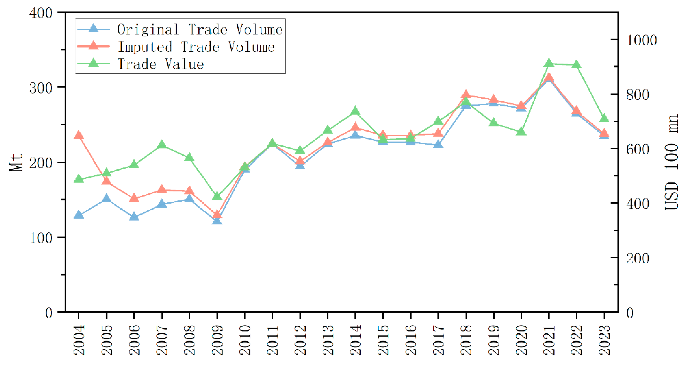
Figure A2.
Global Timber Trade Network: Nodes and Edges (2004-2023).
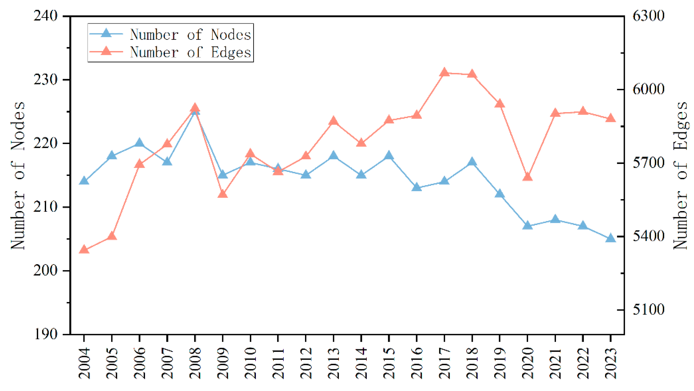
Figure A3.
Global Timber Trade Network: Density and Avg. Path Length (2004-2023).
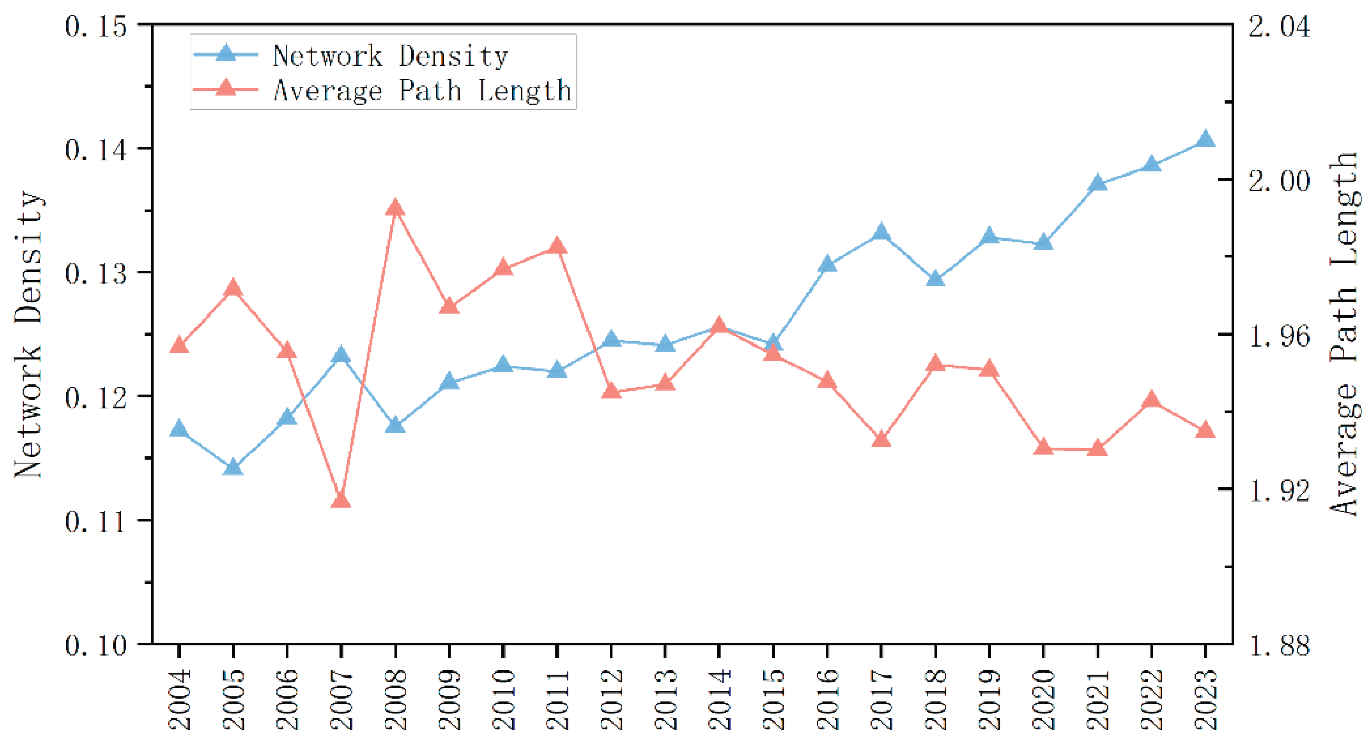
Figure A4.
Global Timber Trade Network Topology (2005-2023).
Appendix B
Table 1.
Key Parameter Description of the Underload Cascading Failure Model.
| Model components | Key parameters (Formula) | Functional explanation | |
| Initial load | Initial load determines node type, underload degree, degradation threshold, and failure threshold. | ||
| Dual-threshold control | α₁ is the degradation threshold and α₂ is the failure threshold. Nodes are grouped according to θᵢ, and within each group, α₁ and α₂ are further linearly interpolated based on θᵢ, preserving inter-group differences while reflecting continuous intra-group distributions. | ||
| Degradation Function |
= Export degradation in cascading failure at step t: |
α₃ is defined as the reciprocal of the logarithmic difference between export and import loads of a node. It modulates the extent of export degradation, with larger differences resulting in greater export degradation. equals the product of underload ratio and α₃; if import load is less than or equal to failure capacity, export is completely interrupted. | |
| Underload Redistribution Algorithm | Importance of trade partnership: |
corresponds to a higher allocation proportion, indicating that supply to less important partners is reduced first during degradation. | |
| Dynamic Propagation Mechanism | Edge load in cascading failure at step t+1: | Degradation propagates progressively from upstream nodes to downstream nodes. |
References
- Cao, X. P.; Yang, S.; Huang, X. M.; Tong, J. X. Dynamic Decomposition of Factors Influencing the Export Growth of China’s Wood Forest Products. Sustainability 2018, 10(8), 16. [Google Scholar] [CrossRef]
- Long, T.; Pan, H. X.; Dong, C.; Qin, T.; Ma, P. Exploring the competitive evolution of global wood forest product trade based on complex network analysis. Physica A 2019, 525, 1224–1232. [Google Scholar] [CrossRef]
- Corona, P.; Alivernini, A. Forests for the world. Annals of Silvicultural Research 2024, 49((2)), 80–81. [Google Scholar]
- Köhl, M.; Lasco, R.; Cifuentes, M.; Jonsson, Ö.; Korhonen, K. T.; Mundhenk, P.; Navar, J. D.; Stinson, G. Changes in forest production, biomass and carbon: Results from the 2015 UN FAO Global Forest Resource Assessment. For. Ecol. Manage 2015, 352, 21–34. [Google Scholar] [CrossRef]
- FAO. The State of the World’s Forests 2024; Technical Report; Food and Agriculture Organization of the United Nations: Rome, Italy, 2024. [Google Scholar]
- Cheng, B.D. Reflections on the issue of wood security in china. China Forestry Industry 2022, (12), 34–37. [Google Scholar]
- Tian, G.; Jiang, Q.Q. Social Network Analysis on International Roundwood Trade Pattern in 2005—2014. World For. Res. 2016, 29, 87–91. [Google Scholar] [CrossRef]
- He, C. Complex Network Analysis of Global Timber Trade [D]; Beijing Forestry University: Beijing, 2018. [Google Scholar] [CrossRef]
- Wang, F.; Tian, M.H.; Yin, R.S.; Zhang, Z.Y. Change of global woody forest products trading network and relationship between large supply and demand countries. Resour. Sci. 2021, 43, 1008–1024. [Google Scholar] [CrossRef]
- Zhou, Y. Y.; Cheng, B. D.; You, W. J.; et al. Evolution of global log trade network structure and transition of China’s status. J. Cent. South Univ. For. Technol. 2021, 41(12), 178–186. [Google Scholar] [CrossRef]
- Tian, G.; Li, X. Q.; Du, Y. W. Network Structure of Wood Forest Products Trade Between China and ASEAN Countries. World For. Res. 2022, 35(01), 100–105. [Google Scholar] [CrossRef]
- Li, Y. X.; Tian, M. H.; Guo, L. Q.; Feng, Q. R.; Yu, M. Y. Social network analysis of the trade pattern of wood products. Issues of Forestry Economics 2022, 42((01)), 63–72. [Google Scholar] [CrossRef]
- Wang, R.; Wu, H. M.; Zhe, R.; et al. Complex network analysis of global forest products trade pattern. Can. J. For. Res. 2023, 53(4), 271–283. [Google Scholar] [CrossRef]
- Liu, L.; Chen, Y.; Yu, J.; et al. Analysis of the Trade Network of Global Wood Forest Products and Its Evolution from 1995 to 2020. For. Prod. J. 2024, 74(2), 121–129. [Google Scholar] [CrossRef]
- Gao, L.; Pei, T. W.; Tian, Y. Trade creation or diversion? Evidence from China’s forest wood product trade. Forests 2024, 15(7), 1276. [Google Scholar] [CrossRef]
- Liu, L.; Chen, Y.; Yu, J.; et al. Study on the Resilience of Global Trade Network of Wood Forest Products. Issues For. Econ. 2024, 44(02), 218–224. [Google Scholar] [CrossRef]
- Huang, X. Y.; Wang, Z. W.; Pang, Y.; Tian, W. J.; Zhang, M. Static Resilience Evolution of the Global Wood Forest Products Trade Network: A Complex Directed Weighted Network Analysis. Forests 2024, 15((9)), 24. [Google Scholar] [CrossRef]
- Caschili, S.; Medda, F. R.; Wilson, A. An Interdependent Multi-Layer Model: Resilience of International Networks. Networks and Spatial Economics. 2015, 15(2), 313–335. [Google Scholar] [CrossRef]
- Yuan, X. J.; Ge, C. B.; Liu, Y. P.; et al. Evolution of Global Crude Oil Trade Network Structure and Resilience. Sustainability 2022, 14(23), 16059. [Google Scholar] [CrossRef]
- Ji, G.; Zhong, H.; Nzudie, H. L. F.; et al. The structure, dynamics, and vulnerability of the global food trade network. Journal of Cleaner Production. 2024, 434, 140439. [Google Scholar] [CrossRef]
- Chen, Y. R.; Chen, M. P. Evolution of the global phosphorus trade network: A production perspective on resilience. Journal of Cleaner Production. 2023, 405, 136843. [Google Scholar] [CrossRef]
- Yu, Y.; Ma, D. P.; Wang, Y. Structural resilience evolution and vulnerability assessment of semiconductor materials supply network in the global semiconductor industry. International Journal of Production Economics. 2024, 270, 109172. [Google Scholar] [CrossRef]
- Jiao, B. Measuring the Resilience of International Energy Trade Networks From an Energy Security Perspective. Ind. Technol. Econ. 2024, 43(05), 131–140. [Google Scholar] [CrossRef]
- Zhou, M. J.; Wang, F. Y.; Shao, L. G. Resilience evaluation of the rare earth supply chain in countries (regions) outside China: A case study of NdFeB permanent magnet. Resour. Sci. 2023, 45(09), 1746–1760. [Google Scholar] [CrossRef]
- Zhong, M.; Huan, M. M. Enhancement strategies of crude oil maritime supply chain network resilience under uncertain disturbances. J. Shanghai Marit. Univ. 2024, 45(03), 40–48. [Google Scholar] [CrossRef]
- Chen, W.; Wang, X. R.; Long, Y.; et al. Resilience Evolution of the Trade Networks in Regions along the Belt and Road. Econ. Geogr. 2024, 44(01), 22–31. [Google Scholar] [CrossRef]
- Zuo, Z. L.; Cheng, J. H.; Zhan, C.; et al. Evolution and vulnerability analysis of the global trade pattern in thelithium industry chain. Resour. Sci. 2024, 46(01), 114–129. [Google Scholar] [CrossRef]
- Shen, X.; Guo, H. X.; Cheng, J. H. The resilience of nodes in critical mineral resources supply chain networks under emergent risk: Take nickel products as an example. Resour. Sci. 2022, 44(01), 85–96. [Google Scholar] [CrossRef]
- Li, Y. L. Risk propagation and countermeasures in the global cobalt industry chain based on multi-layer networks [D]; Central South University, 2023. [Google Scholar]
- Hu, P.; Fan, W. L.; Mei, S. W. Identifying node importance in complex networks. Physica A 2015, 429, 169–176. [Google Scholar] [CrossRef]
- Wang, Y.; Chen, L.; Wang, X. Y.; et al. Trade network characteristics, competitive patterns, and potential risk shock propagation in global aluminum ore trade. Frontiers in Energy Research 2023, 10, 1048186. [Google Scholar] [CrossRef]
- Sun, X.; Shi, Q.; Hao, X. Supply crisis propagation in the global cobalt trade network. Resour. Conserv. Recycl. 2022, 179, 106035. [Google Scholar] [CrossRef]
- Zheng, S. X.; Zhou, X. R.; Tan, Z. L.; et al. Preliminary study on the global impact of sanctions on fossil energy trade: Based on complex network theory. Energy for Sustainable Development. 2022, 71, 517–531. [Google Scholar] [CrossRef]
- Yan, J. J.; Guo, Y. Q.; Zhang, H. W. The dynamic evolution mechanism of structural dependence characteristics in the global oil trade network. Energy 2024, 303, 131914. [Google Scholar] [CrossRef]
- Lee, K. M.; Goh, K. I. Strength of weak layers in cascading failures on multiplex networks: case of the international trade network. Sci. Rep. 2016, 6, 26346. [Google Scholar] [CrossRef]
- Zhao, L. F.; Yang, Y. J.; Bai, X.; et al. Structure, Robustness and Supply Risk in the Global Wind Turbine Trade Network. Renew. Sustain. Energy Rev. 2023, 177, 113214. [Google Scholar] [CrossRef]
- Craig, M.; Zhao, J.; Schneider, G.; et al. Net revenue and downstream flow impact trade-offs for a network of small-scale hydropower facilities in California. Environ. Res. Commun. 2019, 1(1), 011001. [Google Scholar] [CrossRef]
- Xiao, J. X.; Xiong, C.; Deng, W.; et al. Evolution Features and Robustness of Global Photovoltaic Trade Network. Sustainability 2022, 14(21), 14220. [Google Scholar] [CrossRef]
- Cai, H. B.; Song, Y. Y. The state’s position in international agricultural commodity trade: A complex network approach. China Agricultural Economic Review 2016, 8(3), 430–442. [Google Scholar] [CrossRef]
- Zhou, W. W.; Feng, R. L.; Han, M. Y.; et al. Evolution characters and regulation impacts within the global scrap rubber trade network. Resources, Conservation and Recycling 2022, 181, 106201. [Google Scholar] [CrossRef]
- Xia, Y. X.; Fan, J.; Hill, D. Cascading failure in Watts-Strogatz small-world networks. Physica A 2010, 389(6), 1281–1285. [Google Scholar] [CrossRef]
- Sansavini, G.; Hajj, M. R.; Puri, I. K.; et al. A deterministic representation of cascade spreading in complex networks. Europhysics. Letters 2009, 87(4), 48004. [Google Scholar] [CrossRef]
- Goh, K. I.; Lee, D. S.; Kahng, B.; et al. Sandpile on scale-free networks. Physical review letters 2003, 91(14), 148701. [Google Scholar] [CrossRef]
- Lee, D. S.; Goh, K. I.; Kahng, B.; et al. Sandpile avalanche dynamics on scale-free networks. Physica A 2004, 338(1–2), 84–91. [Google Scholar] [CrossRef]
- Macdonald, P. J.; Almaas, E.; Barabási, A. L. Minimum spanning trees of weighted scale-free networks. Europhysics Letters. 2005, 72(2), 308–314. [Google Scholar] [CrossRef]
- Kinney, R.; Crucitti, P.; Albert, R.; et al. Modeling cascading failures in the North American power grid. Eur. Phys. J. B 2005, 46(1), 101–107. [Google Scholar] [CrossRef]
- Zhao, J. B.; Wei, Z. N.; Liu, J. K.; et al. Linearized Dynamic Optimal Power Flow Model for Power System. Autom. Electr. Power Syst. 2018, 42(20), 86–92. [Google Scholar] [CrossRef]
- Yang, R.; Wang, W. X.; Lai, Y. C.; et al. Optimal weighting scheme for suppressing cascades and traffic congestion in complex networks. Phys. Rev. E 2009, 79(2), 026112. [Google Scholar] [CrossRef]
- Duan, D. L.; Wu, J.; Deng, H. Z.; et al. Cascading failure model of complex networks based on adjustable load redistribution. Syst. Eng. Theory Pract. 2013, 33(01), 203–208. [Google Scholar]
- Li, C.; Wang, L.; Zhao, J.; et al. The collapse of global plastic waste trade: Structural change, cascading failure process and potential solutions. Journal of Cleaner Production. 2021, 314, 127935. [Google Scholar] [CrossRef]
- Hao, H.; Ma, Z.; Wang, A. Modeling and assessing the robustness of the lithium global trade system against cascading failures. Resour. Policy 2023, 85, 103822. [Google Scholar] [CrossRef]
- Fu, X.; Xu, X.; Li, W. Cascading failure resilience analysis and recovery of automotive manufacturing supply chain networks considering enterprise roles. Physica A 2024, 634, 129478. [Google Scholar] [CrossRef]
- Yin, X.; Tao, Y.; Zhao, X.; et al. Research on Crisis Propagation Effect in International Trade Network Based on Cascading Failure Model: Take Semiconductors as an Example. J. Syst. Sci. Math. Sci. 2024, 44(5), 1389–1411. [Google Scholar] [CrossRef]
- Wang, C.; Yang, H.; Hu, X.; et al. Deciphering iron ore trade dynamics: Supply disruption risk propagation in global networks through an improved cascading failure model. Resour. Policy 2024, 95, 105157. [Google Scholar] [CrossRef]
- Ouyang, X.; Liu, L.; Chen, W.; et al. Systematic Risks of the Global Lithium Supply Chain Network: From Static Topological Structures to Cascading Failure Dynamics. Environ. Sci. Technol. 2024, 58(50), 22135–22147. [Google Scholar] [CrossRef] [PubMed]
- Miao, C. H.; Wan, Y. F.; Kang, M. L.; et al. Topological analysis, endogenous mechanisms, and supply risk propagation in the polycrystalline silicon trade dependency network. Journal of Cleaner Production. 2024, 439, 140657. [Google Scholar] [CrossRef]
Figure 1.
Research Framework.
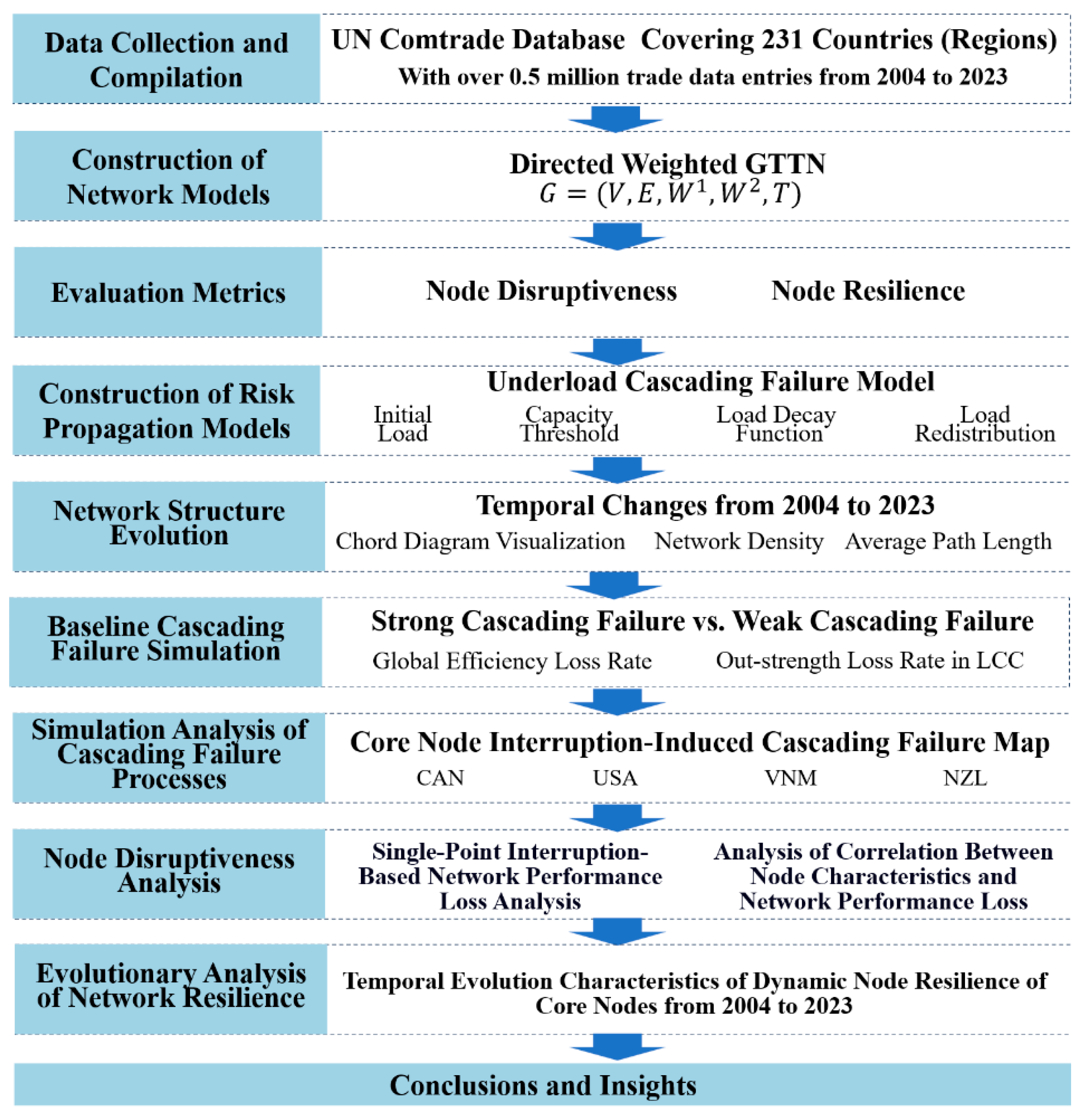
Figure 2.
Cascading failure effects of single-node disruptions: Global efficiency loss analysis.
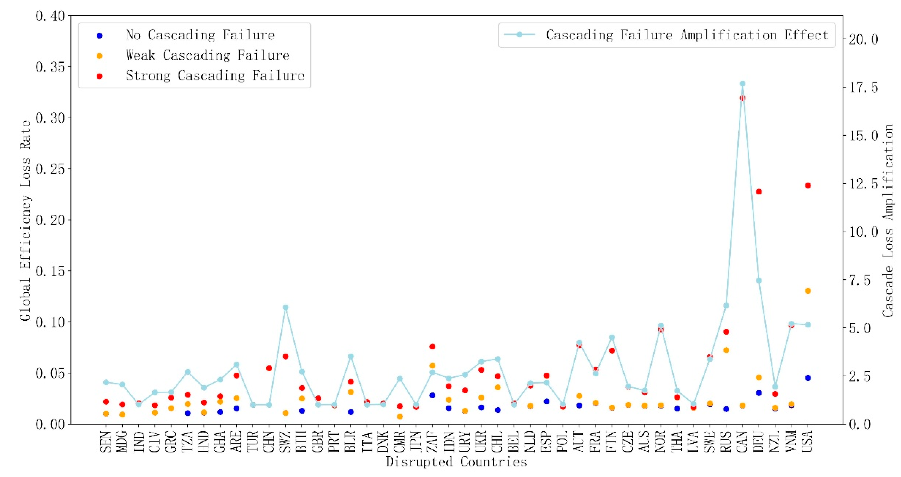
Figure 3.
Cascading failure effects of single-node disruptions: Node strenghth loss rate in LCC.
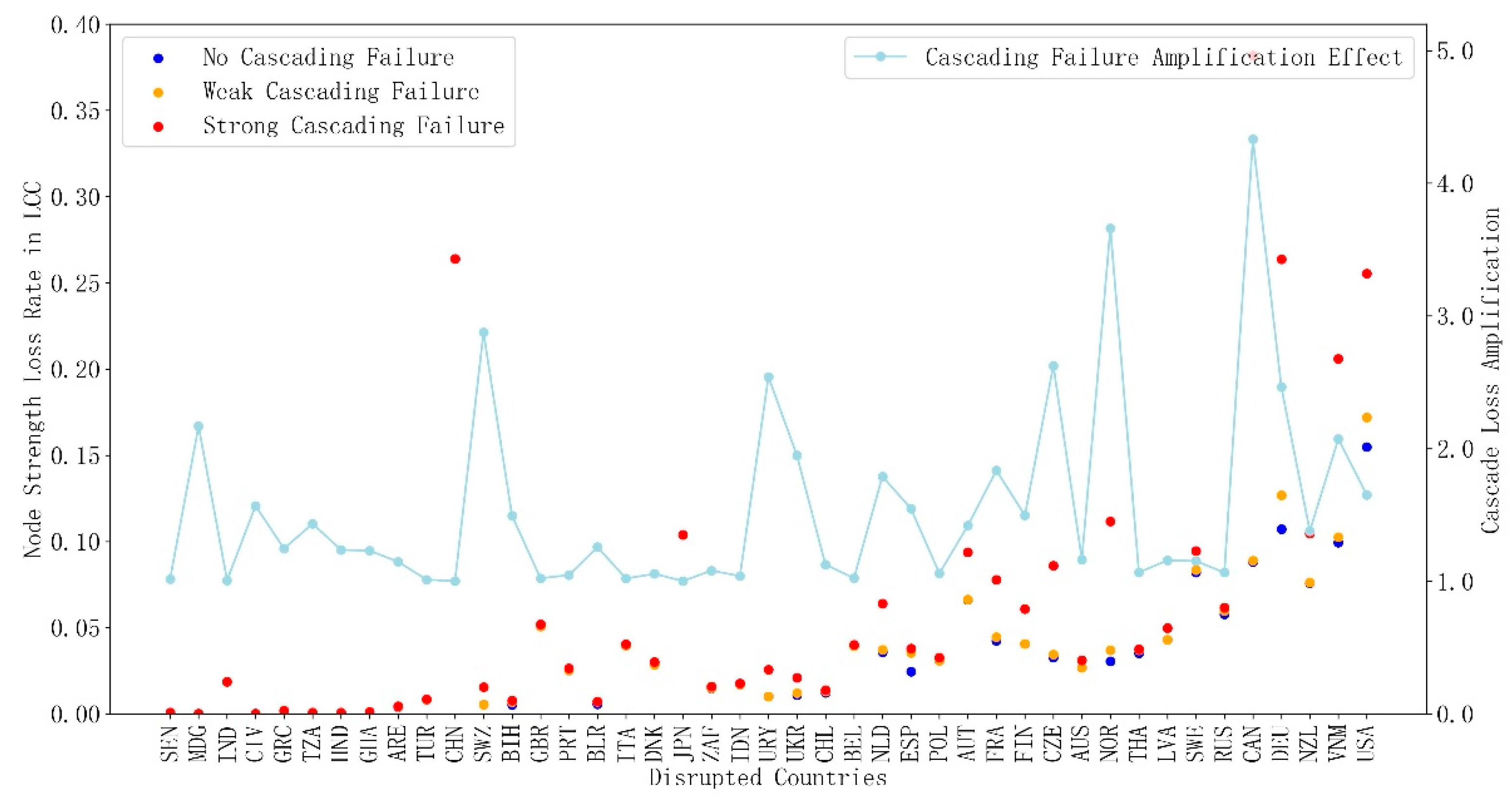
Figure 4.
Propagation map of upload cascading failures following the Canada disruption.
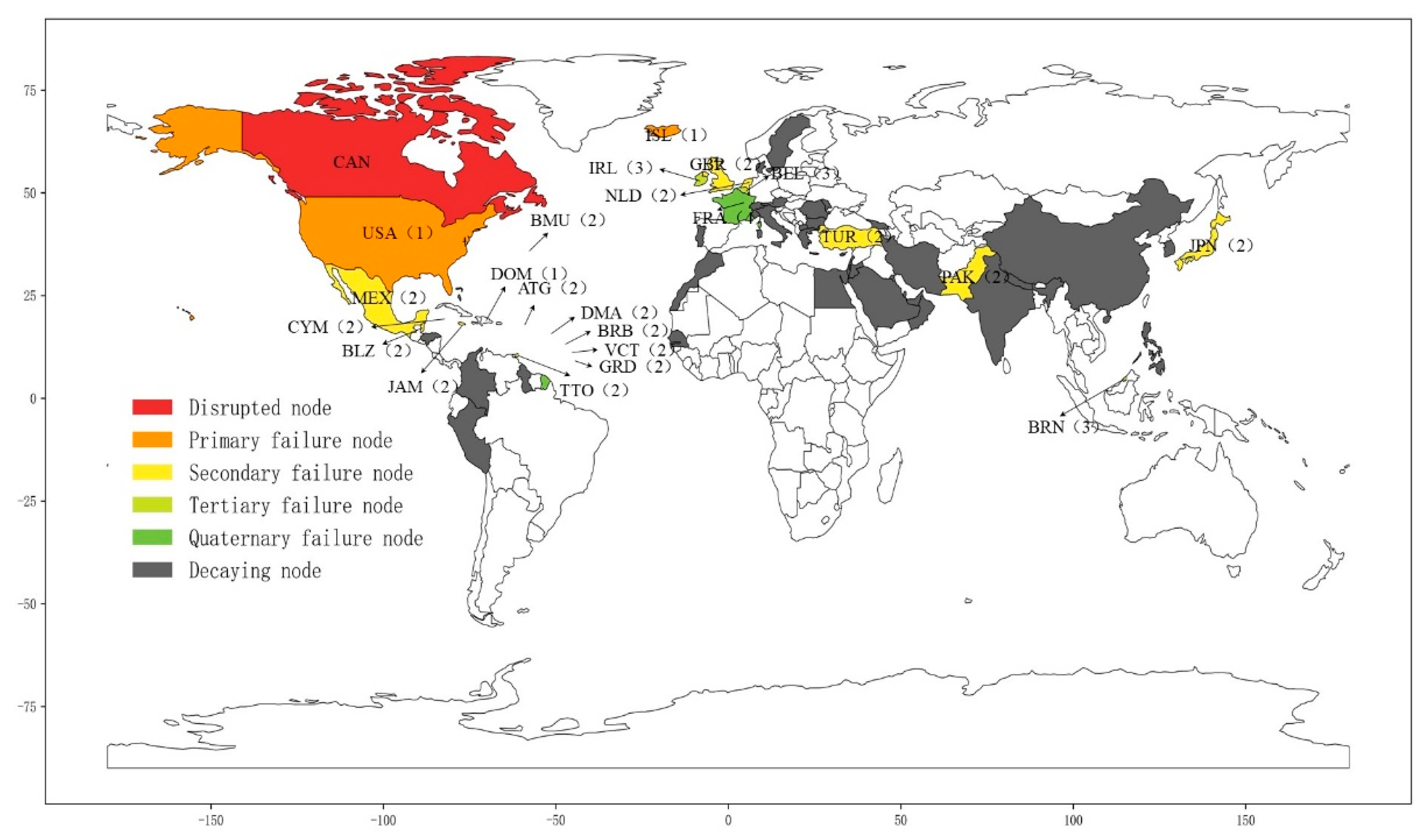
Figure 5.
Propagation map of upload cascading failures following the United States disruption.
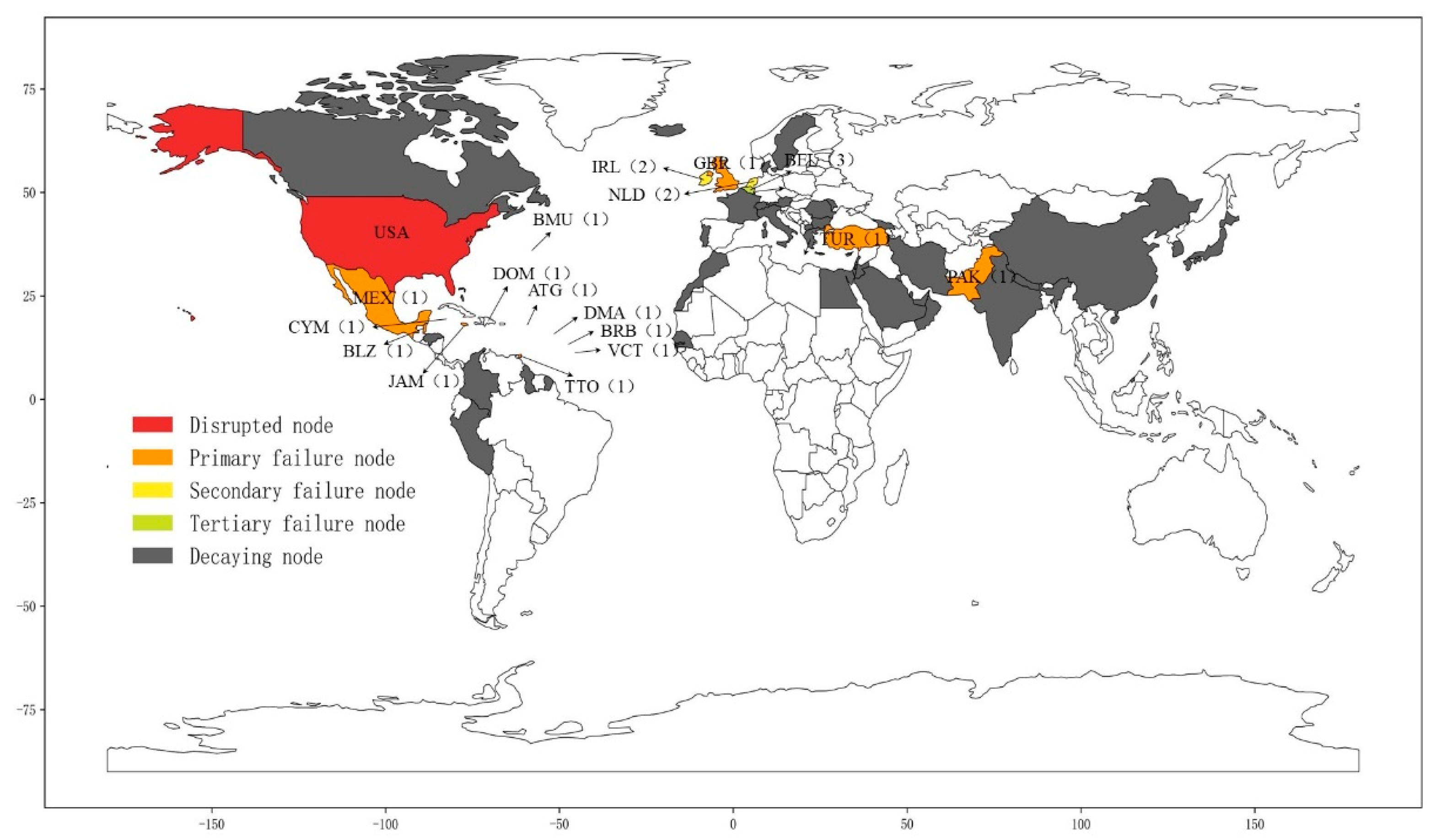
Figure 6.
Propagation map of upload cascading failures following the Vietnam disruption.
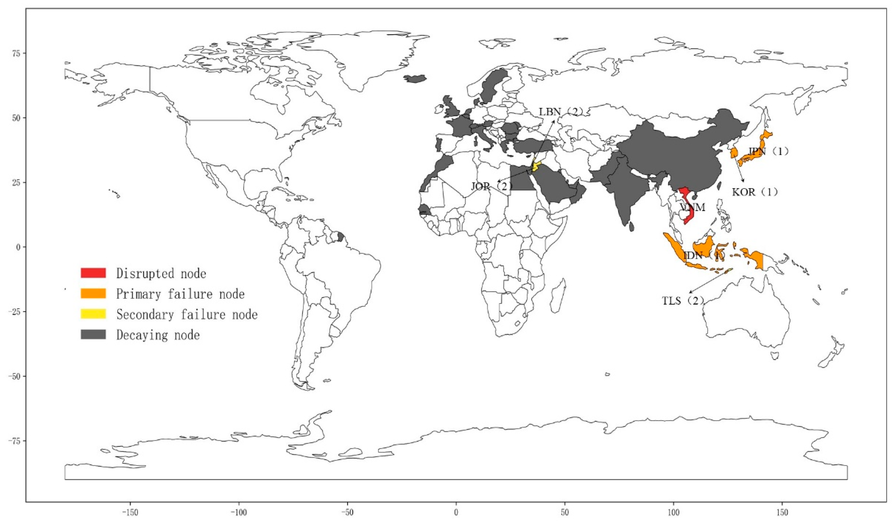
Figure 7.
Propagation map of upload cascading failures following the New Zealand disruption.
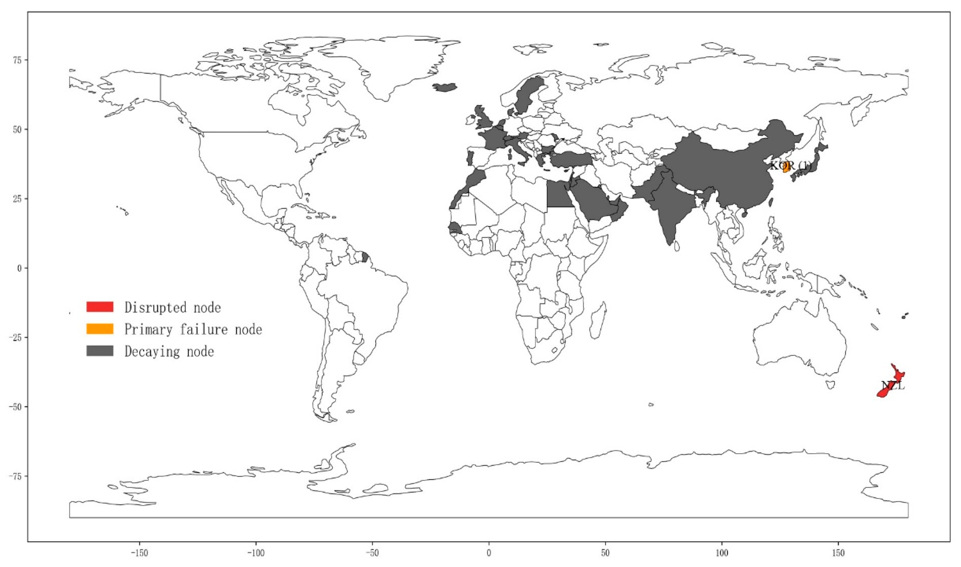
Figure 8.
Core node interruption impact radar chart for network performance loss.
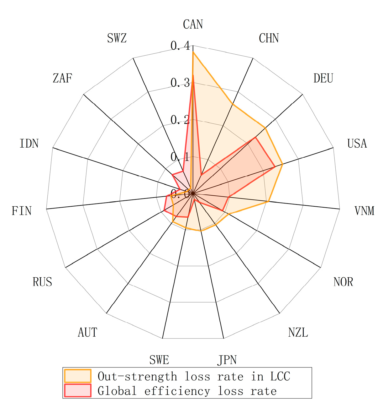
Figure 9.
Correlation coefficient chart of node centrality and network performance loss rate.
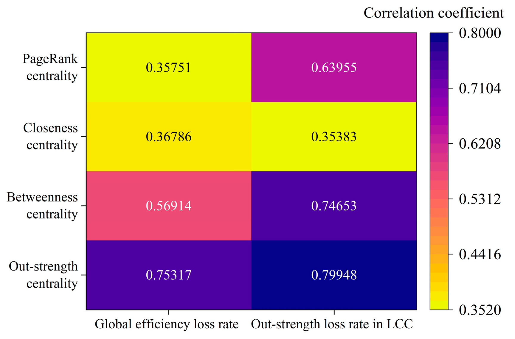
Figure 10.
In-strength retention curves of core nodes under multiple disruption strategies.
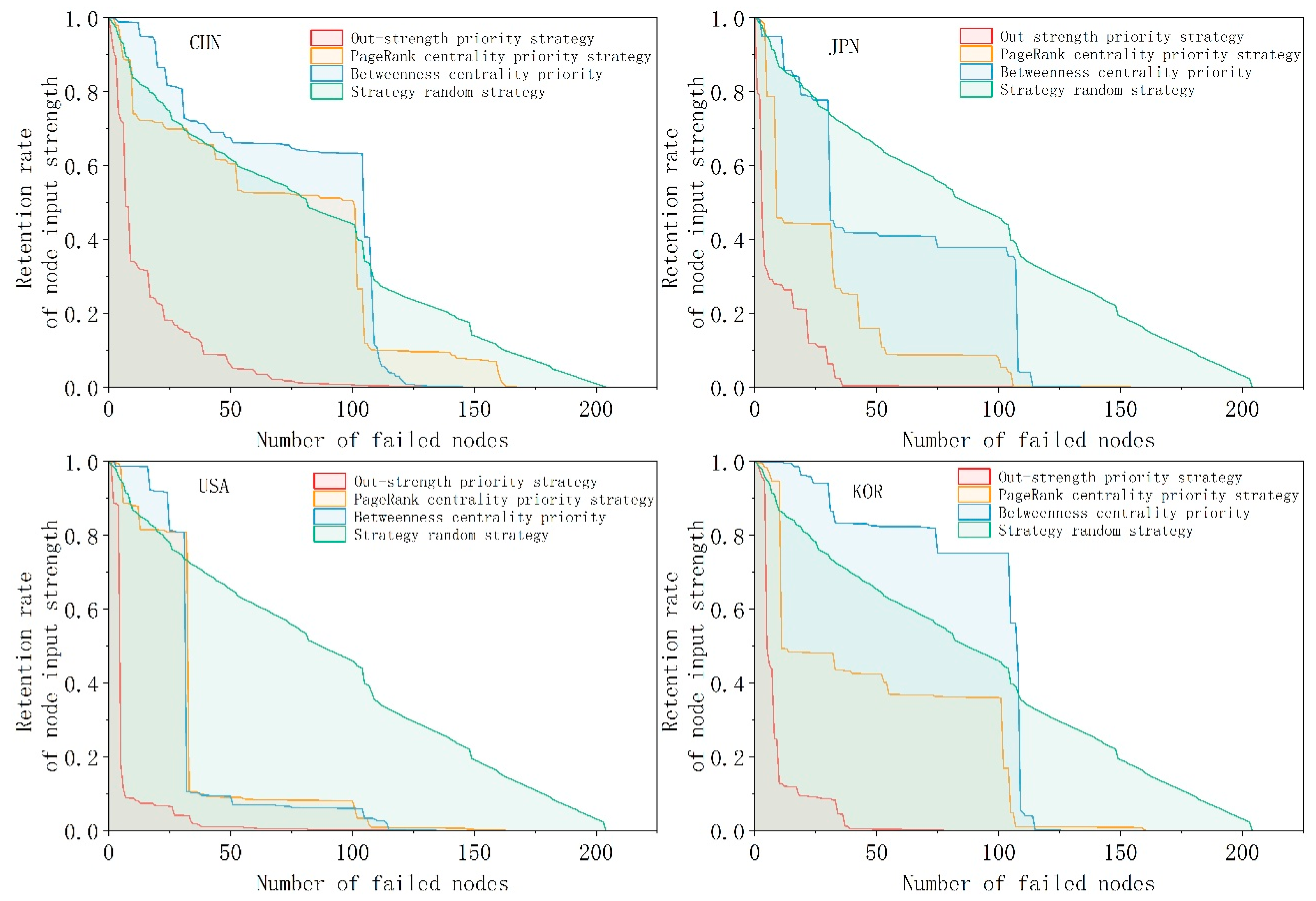
Figure 11.
Comparison of multi-node dynamic resilience under two interruption strategies.
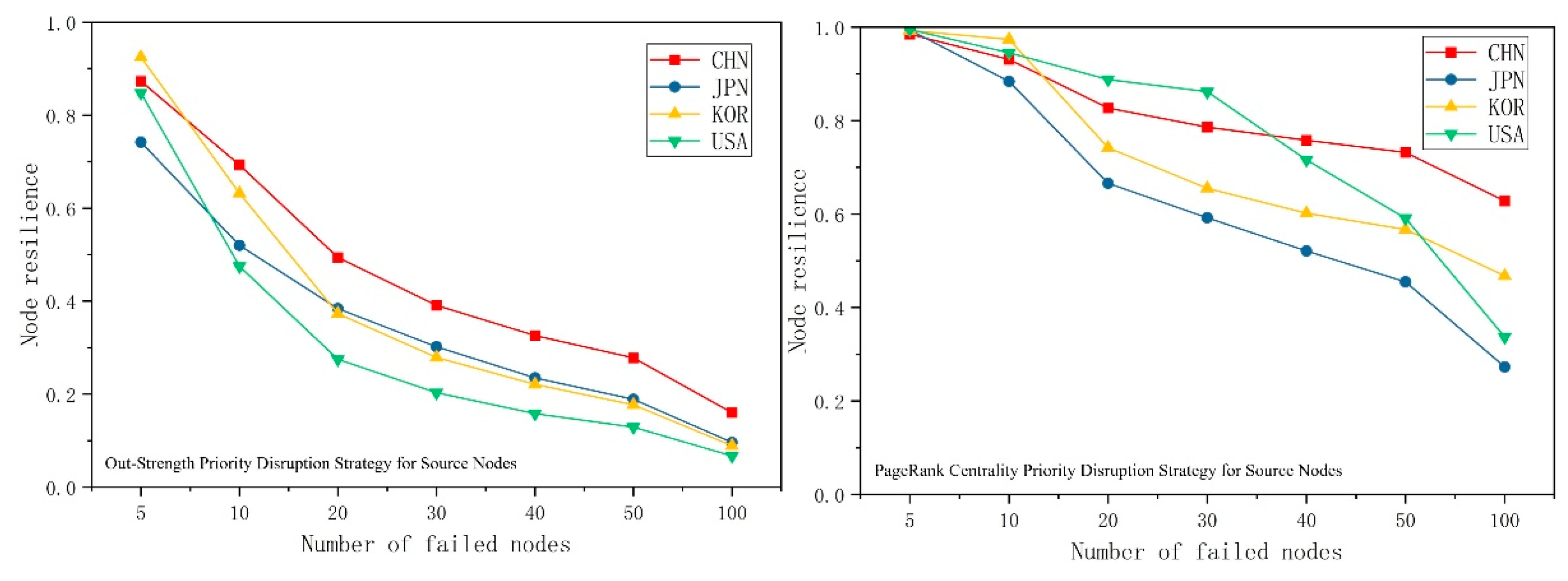
Figure 12.
Evolution of multi-node dynamic resilience trends from 2004 to 2023.
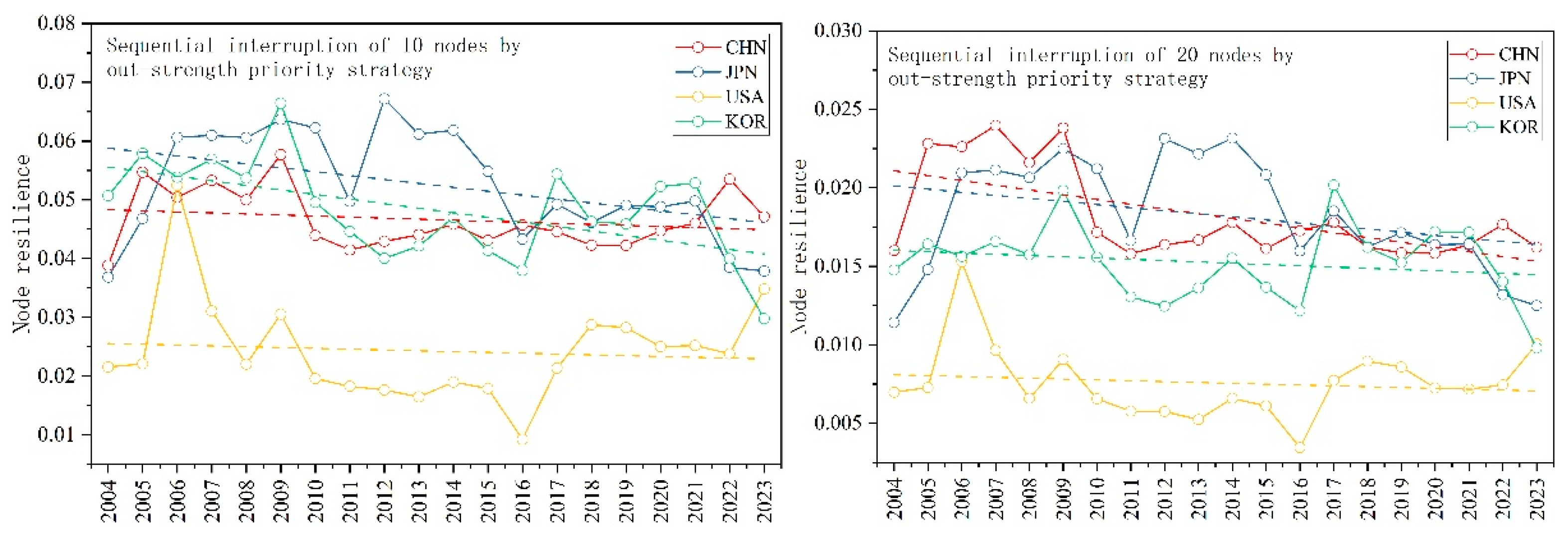
Table 2.
HS codes of timber.
| Product Category | Commodity Code | Detailed Information Regarding HS Codes |
|---|---|---|
| Logs | HS4403 | Wood in the rough. |
| Other Raw Materials |
HS4401, HS4402, HS4404, HS4405 |
Various fuel wood, wood chips/sawdust/waste, wood charcoal, hoop wood/poles/stakes, wood wool/flour. |
| Sawn Timber | HS4406, HS4407 | Wooden sleepers/cross-ties; Sawn/chipped, sliced/peeled wood. |
Table 3.
Complex network metrics.
| Indicator | Formula | Specific Description |
|---|---|---|
| Weighted Global Efficiency | Weighted Global Efficiency measures the efficiency of timber flow within the network. It is defined as the average of the reciprocals of the weighted shortest path lengths between all node pairs, incorporating trade closeness as edge weights. | |
| Out-Strength | Out-Strength denotes the sum of trade volume weights for exports from the node. | |
| In-Strength | In-Strength denotes the sum of trade volume weights for imports to the node. | |
| Weighted Betweenness Centrality |
that pass through node i (considering trade closeness weights) to the total number of weighted shortest paths between all other trade pairs. |
|
| Weighted Closeness Centrality | Weighted Closeness Centrality is calculated as the reciprocal of the average weighted shortest path distance from node i to all other nodes in the network, based on trade closeness weights. | |
| Weighted PageRank Centrality | Weighted PageRank Centrality is a metric used to measure the importance of nodes in a directed network. Its value depends not only on the number and weights of incoming edges, but also on the importance of upstream nodes. In this study, trade volume weights are incorporated into the calculation, meaning that nodes receiving larger timber exports from more important sources are assigned higher centrality values. | |
| Weighted Eigenvector Centrality | Weighted Eigenvector Centrality is a metric that measures the importance of a node in a network, based on the idea that a node’s significance depends on the importance of its neighboring nodes. In this study, the metric is weighted by trade volume, so that each node reflects not only its number of connections but also its influence in terms of timber trade flow. | |
| Pearson Correlation Coefficient | The Pearson correlation coefficient r (range: [-1,1]) quantifies the degree of linear association between two continuous variables, computed as the ratio of covariance to the product of standard deviations. |
Table 4.
Comparison of cascading failure mechanisms: infrastructure networks vs. GTTN.
| Comparison dimension | Infrastructure Networks | GTTN |
|---|---|---|
| Cascading failure type | Overload failure:Node disruption leads to load redistribution to adjacent nodes, resulting in capacity exceedance and subsequent collapse. | Underload failure: Disruption of supply nodes leads to shortages in downstream nodes, triggering export volume degradation. |
| Failure trigger condition | Node or edge disruption results in physical load exceeding capacity limits. | Node or edge disruption results in resource supply falling below the failure threshold. |
| Load redistribution logic |
Uniform or non-uniform selective allocation: More load is allocated to stronger connections. | Non-uniform selective allocation: Lower connection strength corresponds to higher allocation proportion. |
| Failure containment strategy | Faulty nodes are physically isolated. | Dynamic adjustment of downstream export allocation is applied. |
Table 5.
Capacity threshold parameter settings.
| Node grouping | Degradation threshold α₁ | Failure threshold α₂ | |||||||
| Minimum of the group | Minimum of the group | Minimum of the group | Minimum of the group | ||||||
| Strong cascading failure | Weak cascading failure | Strong cascading failure | Weak cascading failure | Strong cascading failure | Weak cascading failure | Strong cascading failure | Weak cascading failure | ||
| Import-dominant type | 0.9 | 0.7 | 1 | 0.8 | 0.6 | 0.4 | 0.7 | 0.5 | |
| Balanced type | 0.5 | 0.3 | 0.9 | 0.7 | 0.2 | 0 | 0.6 | 0.4 | |
| Export-dominant type | 0.5 | 0.3 | 0.5 | 0.3 | 0 | 0 | 0 | 0 | |
Table 6.
Export load decay function for different types of nodes.
| Node Grouping | Export Load Decay Function | Description | |
|---|---|---|---|
| Import-dominant type |
|
,,,。 is defined based on the logarithmic difference between import and export volumes. When,the difference is zero and=1, When,the difference is positive and<1, decreasing as the import-export gap widens. This leads to a higher export decay rate than import decay, reflecting the node’s greater dependence on imports. The parameter enables the model to accurately capture decay differences caused by varying import-export load ratios. |
|
| Balanced type | ), following a proportional decay pattern. | ||
| Export-dominant type | This type of node represents a timber resource-based node, which does not fail due to import disruptions and only experiences a degradation state. |
Table 7.
Propagation extent of underload cascading failures due to single-node disruptions.
| Node Name | Node Out-Strength (Mt) | Betweenness Centrality | PageRank Centrality | Failed Nodes | Degraded Nodes | Number of Affected Countries |
|---|---|---|---|---|---|---|
| CAN | 15.814 | 0.008 | 0.011 | 22 | 43 | 65 |
| USA | 21.854 | 0.028 | 0.138 | 17 | 49 | 66 |
| DEU | 17.117 | 0.031 | 0.071 | 16 | 40 | 56 |
| RUS | 13.261 | 0.001 | 0.009 | 8 | 38 | 46 |
| VNM | 20.603 | 0.020 | 0.010 | 6 | 34 | 40 |
| NOR | 5.875 | 0.004 | 0.004 | 6 | 38 | 44 |
| ZAF | 2.278 | 0.007 | 0.039 | 6 | 43 | 49 |
| FIN | 5.422 | 0.006 | 0.002 | 5 | 37 | 42 |
| AUT | 4.913 | 0.040 | 0.016 | 5 | 40 | 45 |
| SWZ | 0.903 | 0.002 | 0.000 | 5 | 44 | 49 |
| SWE | 8.548 | 0.017 | 0.022 | 4 | 39 | 43 |
| ARE | 0.251 | 0.016 | 0.016 | 3 | 36 | 39 |
| BLR | 1.171 | 0.001 | 0.000 | 3 | 39 | 42 |
| CHL | 2.730 | 0.001 | 0.001 | 3 | 40 | 43 |
| UKR | 2.471 | 0.002 | 0.004 | 3 | 41 | 44 |
| NZL | 17.387 | 0.001 | 0.004 | 1 | 37 | 38 |
| IDN | 2.318 | 0.004 | 0.003 | 2 | 37 | 39 |
| GHA | 0.219 | 0.001 | 0.000 | 2 | 37 | 39 |
| TZA | 0.099 | 0.002 | 0.001 | 2 | 37 | 39 |
| FRA | 5.213 | 0.019 | 0.031 | 2 | 38 | 40 |
Table 8.
Top 30 nodes by performance degradation due to single-node failures.
| Rank | Global Efficiency Loss Rate | Out-Strength Loss Rate in LCC | Rank | Global Efficiency Loss Rate | Out-Strength Loss Rate in LCC | Rank | Global Efficiency Loss Rate | Out-Strength Loss Rate in LCC | ||||||
|---|---|---|---|---|---|---|---|---|---|---|---|---|---|---|
| Node | Value | Node | Value | Node | Value | Node | Value | Node | Value | Node | Value | |||
| 1 | CAN | 0.319 | CAN | 0.382 | 11 | SWZ | 0.066 | AUT | 0.094 | 21 | IDN | 0.037 | ESP | 0.038 |
| 2 | USA | 0.234 | NZL | 0.306 | 12 | SWE | 0.066 | CZE | 0.086 | 22 | CZE | 0.037 | THA | 0.038 |
| 3 | DEU | 0.228 | CHN | 0.264 | 13 | CHN | 0.055 | FRA | 0.078 | 23 | BIH | 0.035 | KOR | 0.035 |
| 4 | VNM | 0.096 | DEU | 0.264 | 14 | FRA | 0.053 | NLD | 0.064 | 24 | URY | 0.033 | POL | 0.033 |
| 5 | NZL | 0.093 | USA | 0.255 | 15 | UKR | 0.053 | RUS | 0.062 | 25 | AUS | 0.031 | AUS | 0.031 |
| 6 | NOR | 0.093 | VNM | 0.205 | 16 | ARE | 0.048 | FIN | 0.061 | 26 | TZA | 0.029 | EST | 0.031 |
| 7 | RUS | 0.090 | NOR | 0.112 | 17 | ESP | 0.048 | GBR | 0.052 | 27 | GHA | 0.027 | DNK | 0.029 |
| 8 | AUT | 0.077 | JPN | 0.104 | 18 | CHL | 0.047 | LVA | 0.050 | 28 | THA | 0.026 | PRT | 0.026 |
| 9 | ZAF | 0.076 | SWE | 0.095 | 19 | BLR | 0.041 | ITA | 0.041 | 29 | GRC | 0.026 | URY | 0.026 |
| 10 | FIN | 0.072 | AUT | 0.094 | 20 | NLD | 0.038 | BEL | 0.040 | 30 | GBR | 0.025 | BRA | 0.021 |
Disclaimer/Publisher’s Note: The statements, opinions and data contained in all publications are solely those of the individual author(s) and contributor(s) and not of MDPI and/or the editor(s). MDPI and/or the editor(s) disclaim responsibility for any injury to people or property resulting from any ideas, methods, instructions or products referred to in the content. |
© 2026 by the authors. Licensee MDPI, Basel, Switzerland. This article is an open access article distributed under the terms and conditions of the Creative Commons Attribution (CC BY) license.
Copyright: This open access article is published under a Creative Commons CC BY 4.0 license, which permit the free download, distribution, and reuse, provided that the author and preprint are cited in any reuse.


