Submitted:
08 January 2026
Posted:
09 January 2026
You are already at the latest version
Abstract
Image datasets characterized by high intra-image structural heterogeneity pose significant challenges for supervised classification, particularly when local patterns contribute unevenly to image-level decisions. In such scenarios, direct image-level learning may obscure relevant local variability and introduce bias in both training and evaluation. This study proposes a statistically guided, patch-based computational pipeline for the automatic classification of elementary morphological patterns, with application to bioelectrographic imaging data. The pipeline is progressively refined through explicit statistical diagnostics, including image-level data splitting to prevent data leakage, class imbalance handling, and decision threshold calibration based on validation performance. To further control structural bias across images, a continuous image-level descriptor, denoted as \textit{pct\_point\_true}, is introduced to quantify the proportion of point-like structures and support dataset stratification and stability analysis. Experimental results demonstrate consistent and robust patch-level performance, together with coherent behavior under complementary image-level aggregation analysis. Rather than emphasizing architectural novelty, the study prioritizes methodological rigor and evaluation validity, providing a transferable framework for patch-based analysis of structurally heterogeneous image datasets in applied computer vision contexts.
Keywords:
patch-based image analysis
; computer vision
; morphological pattern classification
; hierarchical image data
; class imbalance
; decision threshold calibration
; data leakage prevention
; structural variability
; bioelectrographic imaging
1. Introduction
Bioelectrography, also referred to as Kirlian photography or Gas Discharge Visualization (GDV), is an imaging technique based on the capture of high-frequency electrical discharges generated around biological objects subjected to controlled electric fields [1,2,3]. Under controlled acquisition conditions, the resulting images exhibit complex luminous patterns, including filamentary structures, branching formations, isolated bright points, and spatial variations in intensity.
Several studies have reported that such visual patterns may be associated with functional or physiological conditions of the organism when analyzed under controlled experimental protocols, including autonomic or psychophysiological responses [2,3]. However, interpretations in this domain remain challenging, and many reported analyses rely on qualitative visual inspection or heuristic descriptors, which are inherently subjective, observer-dependent, and difficult to standardize or reproduce [4,5].
From a computational perspective, bioelectrographic images pose substantial analytical challenges due to their high sensitivity to acquisition conditions and intrinsic structural heterogeneity [6,7]. Variations in contact pressure, positioning, ambient conditions, and device parameters can introduce significant intra- and inter-image variability, complicating the extraction of consistent morphological information. Moreover, a single image may simultaneously contain multiple distinct structural patterns, rendering global image-level descriptors insufficient to capture local morphological diversity [8,9].
Previous computational approaches in related imaging domains have predominantly relied on global image features, such as intensity-based statistics, texture descriptors, or entropy-based measures [6,10]. While such approaches represent important advances toward quantitative analysis, they are limited in their ability to capture local morphological heterogeneity. Aggregating heterogeneous structures into a single global representation may obscure relevant patterns and lead to ambiguous or biased interpretations, particularly in the presence of hierarchical image data [11].
In this context, patch-based computer vision approaches provide a natural and principled alternative. By decomposing images into smaller, morphologically more homogeneous regions, patch-based methods enable localized analysis while preserving spatial diversity [7,12]. This paradigm has been successfully adopted in several domains involving heterogeneous visual data, including biomedical imaging, digital pathology, and materials analysis [8,13,14,15].
Motivated by these considerations, this study proposes a statistically guided, patch-based computational pipeline for the classification of elementary morphological patterns in bioelectrographic images. In this context, line-like and point-like structures are intentionally adopted as minimal and operational morphological primitives, providing a controlled abstraction that reduces semantic ambiguity while preserving the essential structural heterogeneity observed in the data. The focus of the work is methodological rather than clinical: the goal is to assess how principled computer vision and machine learning strategies can be combined to reduce subjectivity, improve reproducibility, and provide statistically sound performance evaluation in the presence of hierarchical and imbalanced image data [11].
The main contributions of this work are threefold: (i) the formulation of a patch-level morphological classification problem explicitly designed to handle intra-image heterogeneity; (ii) the integration of unsupervised and supervised learning stages within a unified and reproducible computational pipeline; and (iii) the adoption of explicit statistical diagnostics, including data leakage prevention, class imbalance handling, and decision threshold calibration, to ensure robust and interpretable evaluation [16,17,18].
2. Complete Methodological Description of the Proposed Pipeline
2.1. Computational Formulation of the Problem
The objective of the proposed pipeline is the automatic identification and classification of elementary morphological patterns in bioelectrographic images using computer vision and deep learning techniques. These images originate from electrical discharge phenomena and are characterized by complex spatial structures and strong intra-image heterogeneity [8,19].
The classification task focuses on distinguishing two elementary morphological categories: predominantly linear structures (lines) and localized point-like structures (points). Importantly, these categories are not mutually exclusive at the image level. A single bioelectrographic image may simultaneously contain long filaments, fragmented linear segments, isolated luminous points, and regions with sparse activity [4,6].
In this formulation, the analysis is shifted from global image labels to localized image regions, enabling the explicit modeling of intra-image structural heterogeneity.
This characteristic renders a global image-level labeling strategy conceptually inadequate. Assigning a single label to an image obscures local structural diversity, introduces semantic ambiguity, and increases label noise. From a statistical standpoint, such formulations are known to produce optimistic performance estimates, particularly in hierarchical datasets, where local instances share image-specific acquisition artifacts [7,9,11].
To address these limitations, the problem is reformulated at the local level using a patch-based approach. Each bioelectrographic image is decomposed into multiple patches corresponding to connected components extracted after preprocessing and structural enhancement. Each patch is assumed to predominantly represent a single elementary morphological structure, enabling the classification task to be formulated as a supervised binary problem at the patch level. Comparable formulations are well established in hierarchical, multiple-instance, and weakly supervised learning settings involving heterogeneous visual data [11,13].
2.2. Overview of the Methodological Pipeline
Figure 1 provides a schematic overview of the proposed computational pipeline.
The pipeline consists of a sequence of interdependent stages designed to address specific methodological challenges. Raw images are first preprocessed and structurally enhanced to highlight morphological patterns of interest. Connected components are then extracted to form patches, which serve as the fundamental units for subsequent analysis [8,12].
To support consistent labeling and reduce subjectivity, unsupervised clustering is employed as an intermediate organizational step. The resulting patches are subsequently used to train a supervised convolutional neural network classifier. Throughout the pipeline, explicit mechanisms are incorporated to prevent data leakage, handle class imbalance, and calibrate the classifier decision policy, following best practices for hierarchical and imbalanced imaging datasets [9].
2.3. Intrinsic Challenges of Morphological Classification
Morphological classification in bioelectrographic images presents challenges that extend beyond those encountered in conventional natural image classification. These challenges arise from three primary factors: pronounced class imbalance, hierarchical data structure, and substantial variability in structural composition across images [5,8].
2.3.1. Imbalance between Morphological Classes
Exploratory analysis revealed a strong natural imbalance between morphological classes, with line-type structures substantially outnumbering point-like structures. In such scenarios, global accuracy becomes weakly informative, as it can be dominated by the majority class [16,21]. Consequently, evaluation must rely on metrics that are sensitive to minority-class behavior, such as precision, recall, and F1-score [17,22].
2.3.2. Impact of Imbalance on Training and Decision-Making
Class imbalance affects both training and inference. During optimization, standard loss functions tend to favor the majority class, potentially leading to classifiers with limited sensitivity to point-like structures. At inference time, fixed decision thresholds may place the classifier in suboptimal operating regimes. These effects highlight the conceptual distinction between representation learning and decision policy specification [18,23].
2.3.3. Structural Variability across Images
In addition to patch-level heterogeneity, substantial variability is observed across individual bioelectrographic images. While some images are dominated by linear structures, others exhibit a markedly higher proportion of point-like patterns. Similar inter-image variability has been consistently reported in other biomedical and scientific imaging domains characterized by heterogeneous spatial organization [8,14,15].
This variability has direct methodological implications. When images differ substantially in their internal structural composition, patch-level performance metrics aggregated across the dataset may implicitly weight images unevenly, depending on their prevalence of specific morphological patterns. As a consequence, datasets composed of structurally heterogeneous images cannot be assumed to contribute homogeneously to global performance estimates, particularly in hierarchical settings where local instances are not statistically independent [9,11].
To enable a systematic and interpretable characterization of this inter-image variability, an image-level structural descriptor is introduced. The metric, denoted as pct_point_true, represents the proportion of patches labeled as point-like structures relative to the total number of patches extracted from a given image. Importantly, this metric is not used for model training or inference; it serves exclusively as a descriptive and analytical tool for structural analysis, dataset stratification, and image-level interpretation.
By construction, pct_point_true is computed exclusively from ground-truth patch labels and is therefore independent of classifier predictions. As such, it provides a structural descriptor of the dataset rather than a performance-dependent quantity [9,11]. The formal definition of this metric, together with its empirical distribution and methodological role in image-level analysis, is presented in Section 6.
The introduction of this descriptor establishes an explicit link between patch-level classification and image-level behavior, supporting the subsequent evaluation of model stability under structurally heterogeneous data conditions and reinforcing the need for hierarchical analysis strategies in bioelectrographic imaging.
2.4. Methodological Implications
The considerations discussed in this section demonstrate that bioelectrographic image analysis cannot be treated as a conventional image-level classification problem. The coexistence of multiple structures within a single image, combined with class imbalance and inter-image variability, necessitates a carefully structured methodological framework [9,11].
These principles motivate all subsequent methodological decisions adopted in this study, including patch-level dataset construction, prevention of data leakage through image-level splitting, imbalance-aware training strategies, and explicit calibration of the classifier decision policy. Together, they establish a statistically sound and reproducible foundation for the experimental analyses presented in the following sections.
3. Dataset Construction and Labeling Strategy
The dataset construction stage is central to the proposed pipeline, since decisions made at this level directly affect the statistical validity of subsequent experiments and the generalization capability of the trained models [8,11]. This section describes the data origin, dataset volumetry, operational labeling criteria, class distribution, and the protocol adopted to ensure semantic consistency and reproducibility.
3.1. Operational Definitions of Morphological Patterns
Given the high intra-image heterogeneity of bioelectrographic images, the supervised task in this study relies on explicit operational definitions of the morphological patterns of interest [4,8]. These definitions are intended to support consistent annotation and reproducibility, rather than to provide an exhaustive physical interpretation of the underlying discharge phenomena.
Two elementary morphological classes are considered at the patch level: line and point. Importantly, these definitions are applied exclusively to patches extracted from each image; no global image-level label is assigned during dataset construction [11].
A line pattern is defined as a luminous structure exhibiting clear directional continuity across multiple pixels within a patch. Operationally, line patterns are characterized by elongated geometries with a dominant orientation, such that their spatial extent along one principal axis is substantially greater than along the orthogonal axis [4,12]. Minor discontinuities caused by noise or thresholding artifacts are tolerated, provided that the overall filamentary structure remains visually and structurally coherent.
A point pattern is defined as a localized luminous structure with limited spatial extent and no dominant orientation. These structures typically appear as compact and approximately isotropic clusters of activated pixels [8,10]. Short or fragmented structures that do not exhibit sustained directional continuity are classified as points, even when their local intensity is comparable to that of line structures.
These operational definitions explicitly acknowledge that a single bioelectrographic image may contain a heterogeneous mixture of line-like and point-like structures. By enforcing classification at the patch level, the formulation avoids semantic ambiguities associated with assigning a single label to a structurally heterogeneous image [9,11].
3.2. Data Origin and Dataset Volumetry
The dataset analyzed in this study is composed of 2,000 independent bioelectrographic images, each identified by a unique image_id. After the preprocessing and structural enhancement stages described previously, a total of 191,964 patches corresponding to connected components detected in the binary representations were extracted.
Patch extraction yielded an average of 95.98 patches per image, with a standard deviation of 25.13, reflecting substantial structural variability across images [8,14]. The minimum number of patches per image was 3, while the maximum reached 200, indicating that some images exhibit sparse structures whereas others present dense and complex discharge patterns.
The dataset volumetry is summarized in Table 1.
3.3. Labeling Strategy and XOR Consistency Rule
Patch labeling was performed according to the operational definitions in Section 3.1, distinguishing between predominantly linear (line) and predominantly point-like (point) structures.
To reduce semantic ambiguity and improve label reliability, a mutual exclusion rule based on an exclusive-or (XOR) principle was adopted [5,11]. A patch was considered valid for supervised training only if it exhibited exactly one of the two possible labels: line or point. Patches simultaneously marked as both classes, as well as patches without explicit marking, were excluded from the supervised dataset.
This deterministic filtering step reduces label noise and prevents semantically ambiguous instances from degrading the learning process [4,8,24]. Although such filtering may reduce the number of available samples, it increases label precision, which is critical for fine-grained morphological classification.
After applying the XOR rule, the final supervised dataset retained 191,964 valid patches, distributed as reported in Table 2.
3.4. Initial Analysis of Class Imbalance
The resulting class distribution reveals a pronounced imbalance: approximately 81.94% of patches belong to the line class, whereas only 18.06% correspond to the point class (Table 2). This asymmetry reflects an intrinsic characteristic of the dataset, consistent with the predominance of filamentary structures in the analyzed bioelectrographic images.
From a statistical standpoint, this imbalance has direct implications for model training and evaluation. Global metrics such as accuracy can become weakly informative, as they may be inflated by trivial decision rules favoring the majority class [16,21]. For example, a classifier that always predicts line would achieve high accuracy while failing completely to detect point-like structures.
Figure 2 provides a visual summary of the patch-level class imbalance.
3.5. Reproducibility and Dataset Construction Protocol
All dataset construction and labeling procedures were designed to ensure reproducibility and experimental transparency [9,25]. The dataset statistics reported in this section—including volumetry (Table 1), class distribution (Table 2), and imbalance visualization (Figure 2)— are invariant across all experiments presented in subsequent sections.
To prevent data leakage in the presence of hierarchical data (multiple patches per image), dataset partitioning into training, validation, and test sets must be performed exclusively at the image level, using image_id as the grouping key. Under this protocol, all patches extracted from a given image are assigned to the same subset, ensuring strict independence between splits with respect to acquisition-specific artifacts and image-dependent characteristics [9].
All stochastic processes involved in dataset splitting and model training should be controlled via fixed random seeds. The XOR-based consistency rule is applied deterministically prior to splitting, ensuring that no information from validation or test data can influence dataset construction.
No resampling or artificial balancing is applied at the data level. The observed imbalance is treated as an intrinsic property of the dataset and is explicitly addressed during model training and evaluation through strategies described later in the manuscript. This protocol is essential to attribute performance differences to methodological refinements rather than artifacts introduced during dataset preparation.
The dataset construction protocol described in this section establishes a statistically sound and reproducible foundation for subsequent experiments. However, the effectiveness of the proposed patch-based formulation critically depends on the quality and consistency of the preprocessing and structural enhancement steps used to extract morphologically meaningful patches from raw bioelectrographic images.
Given the pronounced variability in image quality, luminance distribution, and structural composition across the dataset, careful preprocessing is required to ensure that extracted patches accurately represent elementary morphological patterns rather than acquisition artifacts or background noise. The following section therefore details the preprocessing pipeline and patch extraction procedures adopted to operationalize the dataset construction principles defined above.
4. Materials and Methods
This section describes the methodological components of the proposed patch-based computational pipeline. All procedures are reported with an emphasis on reproducibility, experimental transparency, and strict separation between methodological design and quantitative results, which are presented exclusively in subsequent sections [8,9].
To ensure full experimental reproducibility, all preprocessing, patch extraction, training, and decision hyperparameters were fixed a priori and kept constant across all experiments. For completeness and transparency, the full configuration is summarized in Table 3.
4.1. Image Preprocessing and Patch Extraction
Bioelectrographic images exhibit substantial variability in luminance distribution, background artifacts, and structural density, which hinders direct automated analysis. Similar challenges have been reported in heterogeneous biomedical and scientific imaging domains [4,8]. To standardize image representations and isolate morphologically relevant structures, a dedicated preprocessing pipeline was applied prior to patch extraction.
Each image was first resized by constraining its larger spatial dimension to 900 pixels, while preserving the original aspect ratio. Images were then converted to grayscale and smoothed using a two-dimensional Gaussian filter to attenuate high-frequency noise while preserving structural transitions associated with discharge patterns [6,26]. The Gaussian filter standard deviation was fixed across all experiments to ensure methodological consistency.
The region of interest (ROI) corresponding to the discharge halo was automatically identified through percentile-based thresholding followed by morphological operations designed to ensure topological continuity, a strategy commonly adopted for isolating relevant structures in noisy imaging environments [27,28]. The largest connected component was retained as the dominant halo region. To reduce boundary artifacts, an inner halo region was obtained via controlled morphological erosion, excluding external borders that are more susceptible to noise and illumination variability [27].
Structural enhancement was performed using a Difference of Gaussians (DoG) operator, which emphasizes high spatial-frequency components such as filamentary and point-like structures [29,30,31]. The DoG response was restricted to the inner halo ROI and binarized using an adaptive thresholding scheme based on luminance percentiles computed within the ROI. Morphological post-processing and area-based filtering were subsequently applied to suppress residual artifacts and spurious detections [27].
A representative illustration of the preprocessing pipeline and its visual effect on a bioelectrographic image is shown in Figure 3. This figure provides a qualitative reference for the transformation from the raw acquisition to the binary structural representation used for patch extraction.
Connected components extracted from the resulting binary masks were treated as individual patch instances. Each patch corresponds to a morphologically homogeneous structure and constitutes the basic unit of analysis for all subsequent learning stages, consistent with patch-based formulations adopted in biomedical image analysis [8]. Patch extraction was performed deterministically using bounding boxes enclosing each connected component, with fixed preprocessing applied prior to resizing for CNN input [6].
4.2. CNN Architecture and Training Protocol
Patch-level classification was implemented using a convolutional neural network (CNN) architecture based on transfer learning [20]. A backbone network pre-trained on the ImageNet dataset was employed as a feature extractor, enabling the reuse of generic visual representations while reducing training complexity and the risk of overfitting [32,33,34].
All extracted patches were resized to match the input dimensions required by the selected CNN architecture and normalized according to the preprocessing protocol associated with the pre-trained weights. Feature extraction was performed through the convolutional layers of the backbone network, followed by a global average pooling operation to obtain a compact feature representation [35].
A lightweight classification head composed of fully connected layers was appended to the backbone. The final output layer employed a sigmoid activation function to produce probabilistic estimates for the point class. During training, the backbone network weights were kept frozen, and only the parameters of the classification head were optimized, a strategy commonly adopted when training data are limited [8,32]. A schematic overview of the adopted CNN architecture is provided in Figure 4.
Model training followed standard optimization procedures for binary classification. Binary cross-entropy loss was used as the objective function, and all hyperparameters were kept fixed across experiments to ensure comparability between methodological configurations [36].
4.3. Data Splitting Strategy and Leakage Prevention
Due to the hierarchical structure of the dataset, in which multiple patches originate from the same bioelectrographic image, explicit precautions were taken to prevent data leakage between training, validation, and test sets [9,37].
Dataset partitioning was performed exclusively at the image level. All patches associated with a given image identifier (image_id) were assigned to the same subset, ensuring that no structural information from a single image could be shared across different experimental splits. This strategy prevents optimistic bias arising from shared acquisition artifacts, luminance patterns, or noise characteristics [9,37].
Images were partitioned into training, validation, and test sets using fixed proportions (70%, 15%, and 15%, respectively). All random processes involved in dataset partitioning were controlled through fixed random seeds to guarantee full reproducibility.
This image-level splitting strategy constitutes a fundamental methodological constraint of the proposed pipeline and was applied consistently across all experiments reported in this study.
4.4. Class Imbalance Handling
Exploratory analysis revealed a pronounced imbalance between morphological classes at the patch level, with a substantial predominance of line-type structures over point-type structures [16,21]. To mitigate the impact of this imbalance during training, class weighting strategies were incorporated into the loss function [38,39,40].
Class weights were computed inversely proportional to class frequencies in the training set, increasing the relative contribution of the minority point class to the optimization process. These weights were applied exclusively during training and did not alter dataset composition or evaluation protocols.
While alternative loss formulations such as focal loss or class-balanced loss have been proposed in the literature to address class imbalance, this study deliberately adopts standard binary cross-entropy with class weighting in order to isolate the effect of imbalance handling without introducing additional loss-specific hyperparameters or confounding optimization dynamics [39,40].
No resampling, undersampling, or synthetic data generation techniques were employed. The observed class imbalance was treated as an intrinsic property of the dataset and was explicitly addressed through loss reweighting rather than data-level manipulation.
4.5. Decision Threshold Calibration Protocol
The CNN classifier produces probabilistic outputs for the point class, which must be converted into discrete labels for evaluation and downstream image-level analyses. Rather than adopting a fixed and arbitrary decision threshold (e.g., 0.50), an explicit decision threshold calibration protocol was implemented to define the inference-time decision policy in an imbalance-aware manner [17,18].
Threshold calibration was performed exclusively on the validation set to preserve a strict separation between model selection and final evaluation. Candidate threshold values spanning the interval were evaluated, and classifier behavior was quantified using metrics sensitive to class imbalance, with particular emphasis on the F1-score of the minority point class [17]. The threshold that maximized this criterion on the validation set was subsequently fixed and applied to the test set without further adjustment.
This procedure explicitly separates (i) representation learning, governed by the training loss and optimization dynamics, from (ii) the decision policy, defined at inference time by a calibrated threshold [18]. In other words, calibration does not modify the learned feature representations or network parameters; it only specifies the operational rule used to map probabilities into class assignments.
5. Results
This section presents the experimental results obtained from the proposed patch-based classification pipeline, following the methodological procedures described in Section 4 [9]. Results are reported at both the patch level and the image level, with particular attention to the effects of data leakage prevention, decision threshold calibration, and class imbalance handling [16,18]. Unless otherwise stated, all reported results correspond to the test set and were obtained without any post hoc adjustment.
5.1. Impact of Image-Level Data Splitting
The first set of results assesses the impact of correcting data leakage arising from patch-level data splitting. As discussed in Section 4.3, assigning patches from the same image to different subsets can lead to optimistic bias, as shared image-specific characteristics may be inadvertently exploited by the classifier [9,37].
Table 4 reports the patch-level performance obtained before and after enforcing image-level data splitting, using a fixed decision threshold of 0.50. The comparison highlights a moderate reduction in global performance metrics after leakage correction, which is expected and reflects a more realistic estimation of generalization performance under hierarchical dependencies [9,37].
Note: Acc. = accuracy; Prec. (P) = precision for the point class; Rec. (P) = recall for the point class; F1 (P) = F1-score for the point class; Supp. (P) = number of point-class samples in the test set; FP (L→P) = false positives (line misclassified as point); FN (P→L) = false negatives (point misclassified as line).
5.2. Decision Threshold Calibration Results
Following leakage correction, classifier decisions were initially governed by a fixed probability threshold of 0.50. Given the pronounced class imbalance, this choice is arbitrary and may position the classifier in a suboptimal operating regime [17,22].
An explicit threshold calibration procedure was therefore applied using the validation set, as described in Section 4.5. Candidate thresholds spanning the interval were evaluated, and the threshold maximizing the F1-score of the point class was selected and subsequently applied to the test set without further adjustment [18,41].
Figure 6 presents the validation-based calibration curves, showing the evolution of precision, recall, and F1-score for the point class across different threshold values. The selected operating points correspond to the maxima of the F1-score curves [17].
Figure 6.
Validation-based decision threshold calibration, showing precision, recall, and F1-score of the point class as functions of the decision threshold.
Figure 6.
Validation-based decision threshold calibration, showing precision, recall, and F1-score of the point class as functions of the decision threshold.
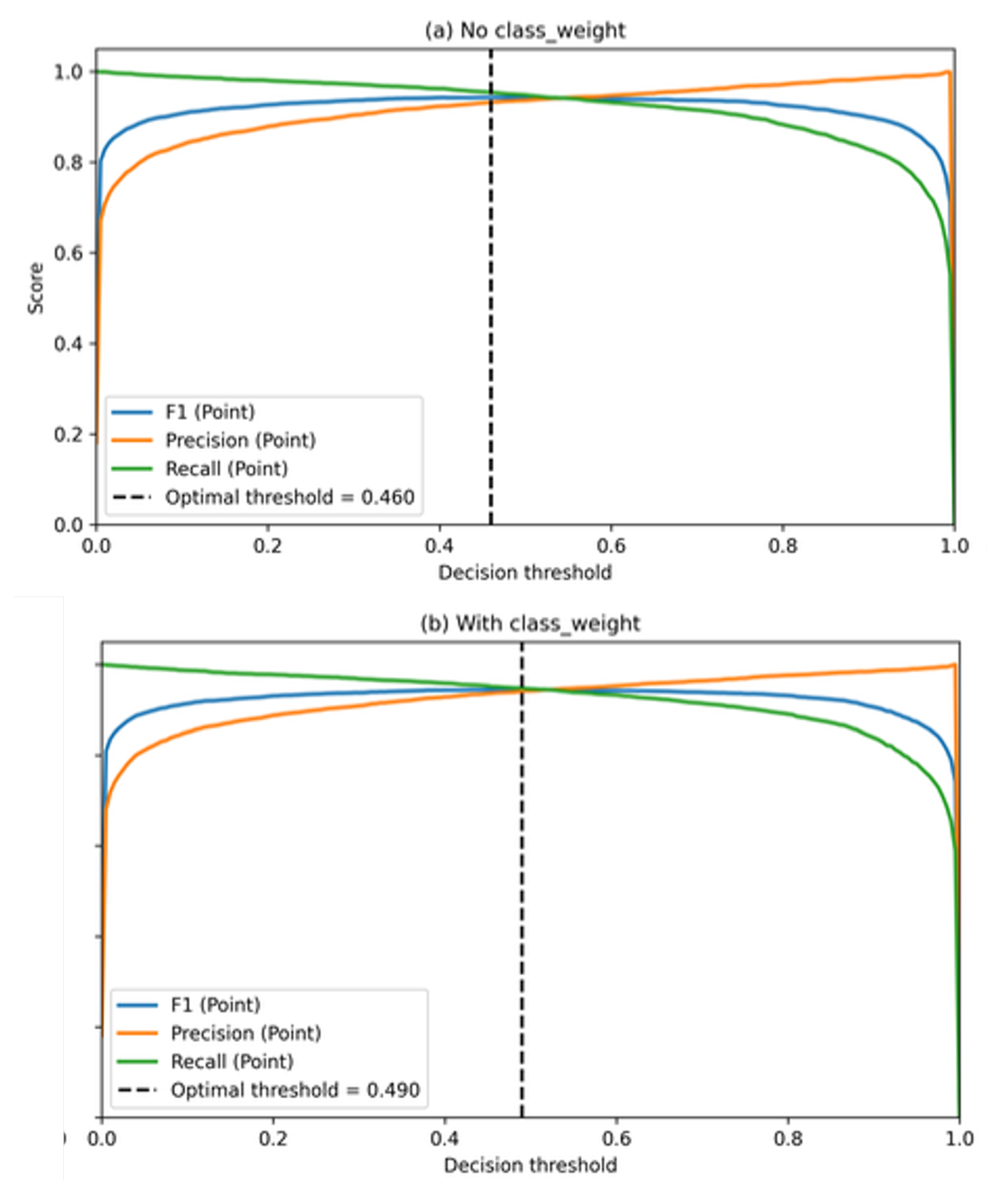
Table 5 summarizes the optimal thresholds selected for the configurations without and with class weighting, together with the corresponding point-class performance on the validation set.

Table 5.
Optimal decision thresholds selected on the validation set and corresponding point-class performance.
Table 5.
Optimal decision thresholds selected on the validation set and corresponding point-class performance.
| Configuration | Optimal threshold | Precision (P) | Recall (P) | F1-score (P) |
|---|---|---|---|---|
| No class_weight | 0.460 | 0.932 | 0.954 | 0.943 |
| With class_weight | 0.490 | 0.941 | 0.948 | 0.944 |
Note: Precision (P), Recall (P), and F1-score (P) refer to performance metrics computed for the point class.
Although both optimal thresholds are close to the conventional value of 0.50, the observed differences have a measurable impact on the balance between false positives and false negatives, as further analyzed below [18].
5.3. ROC and Precision–Recall Analysis
To complement threshold-specific evaluations, classifier performance was also analyzed using Receiver Operating Characteristic (ROC) and Precision–Recall (PR) curves. These curves provide a continuous view of classifier behavior across all possible decision thresholds and allow the assessment of intrinsic discriminative capacity [42].
Given the class imbalance, PR curves are particularly informative because they characterize the precision–recall trade-off under varying decision thresholds and are more sensitive to minority-class behavior than ROC curves in highly imbalanced settings [17,22]. Figure 7 and Figure 8 present the ROC and PR curves for the models trained without and with class weighting, respectively.
The high ROC-AUC and PR-AUC values observed in both configurations indicate strong intrinsic separability between line and point classes [17,42]. Importantly, these results demonstrate that threshold calibration operates on an already well-discriminative classifier, refining the decision policy rather than compensating for structural model limitations [18,41].
5.4. Confusion Matrix Analysis
To provide a concrete and interpretable view of classification errors, confusion matrices were computed for both configurations on the test set using a fixed decision threshold of 0.50. This controlled operating point was intentionally selected to isolate the effect of class weighting on the learned decision boundary, independently of decision threshold calibration effects [16,38,39,40]. Figure 9 contrasts the resulting error profiles.
At this fixed operating point, the introduction of class weighting leads to a simultaneous reduction in both false negatives and false positives for the minority point class. This behavior indicates that class weighting improves the intrinsic separability between classes by reshaping the learned decision boundary during training, rather than merely shifting the classifier’s operating point at inference time [16]. Consequently, the observed improvements reflect a genuine enhancement in classification performance, rather than a trade-off between sensitivity and precision.
5.5. Image-Level Aggregation Results
Beyond patch-level evaluation, patch-wise predictions were aggregated at the image level by computing, for each image, the proportion of patches classified as “point”. This image-level descriptor is denoted as and summarizes the structural composition of each image based on model outputs [11].
The suffix “pred” is used to emphasize that this descriptor is derived from model predictions, in contrast to image-level descriptors computed from ground-truth annotations used elsewhere in the study.
Figure 10 presents the distribution of the pct_point_pred descriptor across the training, validation, and test sets. The boxplot visualization highlights comparable central tendency and dispersion among the three data splits, indicating that the image-level partitioning strategy does not introduce structural bias in terms of aggregated morphological composition [9].
The observed variability of pct_point_pred across images confirms that bioelectrographic images are structurally heterogeneous at the image level, even when patch-level classification performance is stable [8]. This image-level descriptor thus provides a complementary and interpretable summary of classifier behavior, bridging patch-wise predictions and higher-level structural analysis [11].
The implications of this aggregation strategy, particularly with respect to inter-image structural variability and dataset stratification, are further examined in Section 6 and 7.
6. Structural Variability Across Images
While the patch-based formulation adopted in this study effectively addresses intra-image heterogeneity, substantial variability is also observed at the inter-image level [8,9]. Different bioelectrographic images exhibit markedly distinct structural compositions, with some images dominated by filamentary (line-like) structures and others characterized by a higher prevalence of point-like patterns. This variability has important methodological implications for dataset stratification, performance stability, and image-level interpretation of patch-based predictions [11].
6.1. Definition of the pct_point_true Metric
To quantitatively characterize structural variability across images, the metric pct_point_true is defined as the proportion of patches labeled as point-like structures relative to the total number of patches extracted from a given image. This metric provides a compact, image-level descriptor that summarizes the structural composition of each bioelectrographic image while preserving the local nature of the underlying patch-based analysis [11].
The metric is formally defined as:
where denotes the number of patches labeled as point-like structures and represents the total number of patches extracted from the corresponding image.
Importantly, this metric is computed exclusively from ground-truth patch labels and is therefore independent of classifier predictions. As such, it serves as a structural descriptor of the dataset rather than a performance-dependent quantity [9].
Throughout this work, we explicitly distinguish image-level prevalence descriptors computed from ground-truth annotations (pct_point_true) from analogous descriptors computed from model predictions (pct_point_pred), in order to avoid ambiguity between dataset structure and classifier behavior.
6.2. Distribution and Interpretation of Structural Variability
Figure 11 presents the empirical distribution of the pct_point_true metric across the analyzed bioelectrographic images. The distribution reveals pronounced inter-image variability, with values spanning a wide range between images predominantly composed of linear structures and images with a substantially higher proportion of point-like patterns [8].
This variability indicates that bioelectrographic images cannot be assumed to contribute homogeneously to aggregated performance metrics. In particular, images with extreme values of pct_point_true alter the effective class prior at the image level and may disproportionately influence patch-level evaluation results, especially when performance is summarized using threshold-dependent measures such as precision, recall, and F1-score [17,22,43].
From a methodological perspective, the observed distribution justifies the use of pct_point_true (or closely related prevalence descriptors) as a stratification variable during dataset partitioning at the image level, as introduced in earlier sections. Such prevalence-aware stratification is aligned with established practices in experimental design and validation protocols aimed at improving split comparability and reducing variance in performance estimates [9,44]. Moreover, it motivates the subsequent integrated analysis of patch-level performance and image-level behavior, addressed in Section 7.
7. Integrated Results Analysis
The results presented in the previous sections demonstrate that robust patch-level classification performance can be achieved through methodological refinements rather than architectural complexity [8,36]. However, an integrated analysis is required to reconcile patch-level performance metrics with image-level structural behavior and to assess the stability of the proposed pipeline under heterogeneous data conditions [9,11].
At the patch level, the combination of image-level data splitting, class imbalance handling, and validation-based threshold calibration resulted in stable and reproducible performance across all evaluated metrics [16,18]. The consistency observed between validation and test sets, together with the high ROC-AUC and PR-AUC values reported in Section 5, indicates that the classifier learned discriminative morphological representations rather than image-specific artifacts [17,42].
Nevertheless, patch-level performance alone does not fully capture the operational behavior of the system when applied to complete bioelectrographic images. As shown in Section 6, individual images exhibit substantial variability in their internal structural composition, as quantified by the pct_point_true metric. This variability directly affects the distribution of patch-level predictions aggregated at the image level and highlights the importance of interpreting classification results within a hierarchical data framework [9,11].
The integration of patch-level predictions into image-level descriptors provides two key insights. First, aggregation attenuates the impact of isolated misclassifications at the patch level, leading to more stable image-level behavior [11]. Second, it enables explicit characterization of structural heterogeneity across images, revealing that similar patch-level performance metrics may correspond to markedly different image-level profiles [8].
From a methodological perspective, these findings emphasize that stability and interpretability are as critical as raw performance metrics in heterogeneous imaging scenarios [9]. A classifier operating at a fixed decision threshold may exhibit comparable F1-scores across datasets while producing substantially different distributions of false positives and false negatives when evaluated at the image level [23]. The explicit separation between representation learning, decision policy calibration, and aggregation strategy adopted in this study enables these effects to be disentangled and analyzed systematically [18].
Importantly, the integrated analysis confirms that the observed improvements are not driven by overfitting or threshold-specific artifacts. Instead, they emerge from a coherent methodological framework that aligns data partitioning, imbalance handling, threshold selection, and hierarchical evaluation [9]. This alignment ensures that performance estimates remain meaningful under realistic deployment conditions, where structural variability across images is unavoidable [8].
Overall, the combined patch-level and image-level analyses support the central premise of this work: in structurally heterogeneous image datasets, methodological rigor and evaluation design play a decisive role in determining classifier reliability [9,11]. These insights provide a direct bridge to the broader interpretation of results and methodological implications discussed in the following section.
8. Discussion
This study investigated the classification of elementary morphological patterns in bioelectrographic images through a patch-based computational pipeline explicitly designed to address structural heterogeneity, class imbalance, and hierarchical data dependencies [8,9,11]. Rather than proposing architectural innovations, the work deliberately emphasized methodological rigor, evaluation validity, and interpretability— dimensions that are frequently underemphasized in applied computer vision studies involving complex and heterogeneous imaging data [36].
A central finding of this work is that substantial gains in classifier reliability can be achieved through careful control of experimental design choices. In particular, the correction of data leakage via image-level splitting proved to be a necessary prerequisite for meaningful performance estimation. Although this correction led to a modest reduction in absolute performance metrics, it resulted in more stable and reproducible behavior, confirming that earlier gains observed under patch-level splitting were partially inflated by shared image-specific information. This observation is fully consistent with prior reports highlighting the risks of hierarchical data leakage in patch-based and medical imaging pipelines [9,37].
The explicit calibration of the decision threshold further demonstrated that classifier performance in imbalanced scenarios cannot be adequately characterized by fixed or conventional operating points [17,22]. Validation-based threshold selection enabled direct and transparent control over the trade-off between sensitivity and precision for the minority class, without altering the underlying learned representations [18]. Importantly, ROC and Precision–Recall analyses confirmed that this calibration operated on a classifier with strong intrinsic discriminative capacity, reinforcing that performance gains arose from decision-policy refinement rather than compensatory effects [42].
The interaction between class weighting and threshold calibration provides an additional methodological insight. While class weighting enhanced sensitivity to point-like structures during training, its effect on false positive rates was strongly dependent on the selected operating threshold. This behavior supports the view that loss reweighting and decision calibration address distinct stages of the learning pipeline and should therefore be considered jointly rather than as interchangeable mechanisms [16,23].
Beyond patch-level performance, the introduction of the pct_point_true metric enabled explicit characterization of inter-image structural variability. The results demonstrated that bioelectrographic images differ markedly in their internal structural composition, even when global acquisition conditions are controlled [8]. This variability has direct implications for evaluation and deployment, as similar patch-level metrics may correspond to qualitatively different image-level behaviors. The aggregation strategy adopted in this study mitigates local classification noise while preserving interpretability, but it simultaneously highlights the need to explicitly account for structural heterogeneity when drawing higher-level conclusions [11].
From a broader perspective, these findings underscore that patch-based learning is not merely a strategy for increasing sample size, but a methodological necessity when dealing with images that contain multiple coexisting morphological patterns. Global image-level labeling in such contexts risks obscuring relevant local structures and introducing semantic ambiguity [4]. By contrast, the hierarchical formulation adopted here enables localized interpretation while still supporting image-level analysis through controlled aggregation [9,11].
Although this study focuses on bioelectrographic imaging, the methodological principles discussed are transferable to other domains characterized by heterogeneous spatial patterns, including biomedical microscopy, remote sensing, and materials imaging [8]. In such settings, the combination of leakage prevention, imbalance-aware evaluation, threshold calibration, and hierarchical analysis provides a robust foundation for statistically defensible computer vision pipelines [9].
Overall, the discussion reinforces the central premise of this work: in applied vision problems involving structurally heterogeneous images, methodological discipline and evaluation design are at least as important as model architecture [11,36]. This perspective directly informs the limitations and implications discussed in the following section.
9. Limitations and Implications
Despite the methodological rigor adopted throughout this study, several limitations must be acknowledged when interpreting the results and considering potential applications of the proposed pipeline. These limitations primarily stem from the nature of the dataset, the scope of the experimental design, and the intended methodological focus of the work [9].
A first limitation concerns the specificity of the analyzed data. The experiments were conducted exclusively on bioelectrographic images acquired under controlled conditions using a single acquisition protocol. Although this constraint enhances internal validity, it limits direct generalization to datasets obtained with different devices, parameter settings, or experimental environments [4,8]. Variations in acquisition conditions may alter luminance distributions, noise characteristics, and structural densities, potentially affecting preprocessing behavior and patch extraction outcomes; such shifts can also amplify methodological pitfalls in biomedical imaging pipelines [37].
A second limitation relates to the binary formulation of morphological patterns. The classification task was restricted to two elementary classes—line-like and point-like structures—defined through operational criteria at the patch level. While this formulation is appropriate for reducing semantic ambiguity and enabling statistical analysis, it does not capture the full spectrum of structural complexity observed in bioelectrographic images, such as branching patterns, transitional forms, or composite structures [4,8]. Extending the framework to multi-class or continuous morphological representations remains an open direction for future work.
The aggregation strategy adopted at the image level also introduces implicit assumptions. Aggregating patch-level predictions into a single image-level descriptor assumes that the proportion of detected structures provides a meaningful summary of image content. Although this approach improves stability and interpretability, it may oversimplify images exhibiting spatially localized or highly heterogeneous structural configurations [11]. Alternative aggregation strategies that incorporate spatial distribution, regional weighting, or multiple-instance formulations may offer a more nuanced characterization of image-level structure [11].
From a methodological standpoint, the study deliberately prioritizes evaluation validity over architectural optimization. As a result, no extensive exploration of alternative network architectures, feature extractors, or training strategies was performed [36]. While this choice strengthens the interpretability and statistical defensibility of the reported results, it leaves open the question of how architectural modifications might interact with the proposed methodological controls, particularly in the presence of hierarchical and imbalanced data [20].
Despite these limitations, the implications of the present work are significant. The results demonstrate that careful handling of data leakage, class imbalance, and decision policy calibration can substantially improve the reliability of patch-based classification pipelines, even without increasing model complexity [9,16,18]. This finding challenges the common tendency to attribute performance gains primarily to architectural novelty and highlights the central role of experimental design and evaluation strategy.
More broadly, the methodological framework proposed here is applicable to a wide range of imaging domains characterized by hierarchical data structures and intra-image heterogeneity, including histopathology, biomedical microscopy, materials imaging, and remote sensing [8,11]. By explicitly separating representation learning, decision calibration, and aggregation, the pipeline provides a transparent and reproducible basis for interpreting classifier behavior under realistic deployment conditions [37].
These considerations motivate future investigations focusing on cross-dataset generalization, extension to richer morphological taxonomies, and integration with domain-specific validation protocols [4,8]. The conclusions drawn in this study should thus be viewed as a foundation for methodologically robust analysis rather than as an endpoint for applied deployment.
10. Conclusions
This study presented a patch-based computational pipeline for the classification of elementary morphological patterns in bioelectrographic images, with a primary focus on methodological rigor, evaluation validity, and interpretability in the presence of structural heterogeneity [8,9,11,37]. By explicitly addressing hierarchical data dependencies, class imbalance, and decision policy design, the proposed framework provides a statistically defensible alternative to conventional image-level classification approaches, which are known to be vulnerable to bias in heterogeneous and hierarchically structured datasets [23].
The results demonstrate that reliable performance can be achieved without architectural novelty when critical methodological issues are systematically controlled [36]. Image-level data splitting proved essential to prevent data leakage and ensure realistic estimates of generalization performance, a requirement increasingly emphasized in recent machine learning guidelines for biomedical imaging [9,37]. Validation-based decision threshold calibration enabled explicit control of the precision–recall trade-off for the minority class, while ROC and Precision–Recall analyses confirmed that these refinements operated on a classifier with strong intrinsic discriminative capacity [17,18,22,42].
Beyond patch-level evaluation, the introduction of an image-level structural descriptor allowed inter-image variability to be explicitly quantified and interpreted. The combined analysis of patch-level and image-level behavior highlighted that similar performance metrics may correspond to distinct structural profiles, reinforcing the importance of hierarchical evaluation strategies in heterogeneous imaging contexts [4,8,11].
Rather than optimizing for maximal performance, this work emphasizes the importance of experimental transparency, reproducibility, and stability. The proposed pipeline demonstrates that careful alignment between data partitioning, imbalance handling, decision calibration, and aggregation strategies is crucial for producing results that are both interpretable and scientifically robust, particularly in settings involving complex spatial variability and class imbalance [9,16].
Although the study is grounded in bioelectrographic imaging, the methodological principles established here are broadly applicable to other domains characterized by complex spatial heterogeneity and hierarchical data structures, such as biomedical microscopy, remote sensing, and materials imaging [4,8,11]. As such, this work contributes a transferable framework for patch-based image analysis that prioritizes methodological soundness over architectural complexity, providing a solid foundation for future research and application-driven studies [36]. In summary, the primary contribution of this work lies not in architectural novelty, but in the systematic integration of leakage-aware data partitioning, imbalance-sensitive evaluation, decision threshold calibration, and hierarchical analysis within a unified and reproducible patch-based framework.
Author Contributions
Conceptualization, R.G.P.P.; methodology, R.G.P.P.; software, R.G.P.P.; formal analysis, R.G.P.P.; investigation, R.G.P.P.; data curation, R.G.P.P.; writing—original draft preparation, R.G.P.P.; writing—review and editing, R.G.P.P.; visualization, R.G.P.P.; supervision, R.G.P.P. All authors have read and agreed to the published version of the manuscript.
Funding
This research received no external funding.
Institutional Review Board Statement
Not applicable.
Informed Consent Statement
Not applicable.
Data Availability Statement
The data presented in this study are not publicly available due to privacy and experimental restrictions.
Acknowledgments
During the preparation of this manuscript, the authors used generative AI tools for language refinement and clarity improvement. The authors reviewed and edited the output and take full responsibility for the content of this publication.
Conflicts of Interest
The authors declare no conflicts of interest.
Abbreviations
The following abbreviations are used in this manuscript:
| CNN | Convolutional Neural Network |
| ROC | Receiver Operating Characteristic |
| PR | Precision–Recall |
| DoG | Difference of Gaussians |
References
- Pehek, J.O.; Kyler, H.J.; Faust, D.L. Image Modulation in Corona Discharge Photography. Science 1976, 194, 263–270. [Google Scholar] [CrossRef]
- Korotkov, K.G.; Matravers, P.; Orlov, D.V.; Williams, B.O. Application of Electrophoton Capture (EPC) Analysis Based on Gas Discharge Visualization (GDV) Technique in Medicine: A Systematic Review. The Journal of Alternative and Complementary Medicine 2010, 16, 13–25. [Google Scholar] [CrossRef]
- Shichkina, Y.; Fatkieva, R.; Sychev, A.; Kazak, A. Method for Detecting Pathology of Internal Organs Using Bioelectrography. Diagnostics 2024, 14, 991. [Google Scholar] [CrossRef]
- Komura, D.; Ishikawa, S. Machine Learning Methods for Histopathological Image Analysis. Computational and Structural Biotechnology Journal 2018, 16, 34–42. [Google Scholar] [CrossRef]
- Zhou, S.; Greenspan, H.; Shen, D. Deep Learning for Medical Image Analysis: A Survey. Neurocomputing 2021, 452, 631–647. [Google Scholar]
- Gonzalez, R.C.; Woods, R.E. Digital Image Processing, 4 ed.; Pearson, 2018. [Google Scholar]
- Wang, J.; Yang, Y.; Chen, X. Patch-based image classification: A review. Pattern Recognition 2019, 88, 32–48. [Google Scholar]
- Litjens, G.; Kooi, T.; Bejnordi, B.E.; et al. A Survey on Deep Learning in Medical Image Analysis. Medical Image Analysis 2017, 42, 60–88. [Google Scholar] [CrossRef] [PubMed]
- Roberts, M.; Driggs, D.; Thorpe, M.; et al. Common Pitfalls and Recommendations for Using Machine Learning to Detect and Prognosticate for COVID-19 Using Chest Radiographs and CT Scans. Nature Machine Intelligence 2021, 3, 199–217. [Google Scholar] [CrossRef]
- Haralick, R.M.; Shanmugam, K.; Dinstein, I. Textural features for image classification. IEEE Transactions on Systems, Man, and Cybernetics 1973, SMC-3, 610–621. [Google Scholar] [CrossRef]
- Carbonneau, M.A.; Cheplygina, V.; Granger, E.; Gagnon, G. Multiple Instance Learning: A Survey of Problem Characteristics and Applications. Pattern Recognition 2018, 77, 329–353. [Google Scholar] [CrossRef]
- Ojala, T.; Pietikäinen, M.; Mäenpää, T. Multiresolution gray-scale and rotation invariant texture classification with local binary patterns. IEEE Transactions on Pattern Analysis and Machine Intelligence 2002, 24, 971–987. [Google Scholar] [CrossRef]
- Campanella, G.; Hanna, M.G.; Geneslaw, L.; et al. Clinical-Grade Computational Pathology Using Weakly Supervised Deep Learning on Whole Slide Images. Nature Medicine 2019, 25, 1301–1309. [Google Scholar] [CrossRef]
- Kather, J.N.; Krisam, J.; Charoentong, P.; et al. Predicting Survival from Colorectal Cancer Histology Slides Using Deep Learning. PLOS Medicine 2019, 16, e1002730. [Google Scholar] [CrossRef] [PubMed]
- Bulten, W.; Pinckaers, H.; van Boven, H.; et al. Automated Deep-Learning System for Gleason Grading of Prostate Cancer Using Biopsies. The Lancet Oncology 2020, 21, 233–241. [Google Scholar] [CrossRef] [PubMed]
- He, H.; Garcia, E.A. Learning from imbalanced data. IEEE Transactions on Knowledge and Data Engineering 2009, 21, 1263–1284. [Google Scholar] [CrossRef]
- Saito, T.; Rehmsmeier, M. The precision–recall plot is more informative than the ROC plot when evaluating binary classifiers on imbalanced datasets. PLOS ONE 2015, 10, e0118432. [Google Scholar] [CrossRef]
- Guo, C.; Pleiss, G.; Sun, Y.; Weinberger, K.Q. On Calibration of Modern Neural Networks. In Proceedings of the 34th International Conference on Machine Learning (ICML); 2017; pp. 1321–1330. [Google Scholar]
- Korotkov, K. Human Energy Field: Study with GDV Bioelectrography; CRC Press, 2012. [Google Scholar]
- LeCun, Y.; Bengio, Y.; Hinton, G. Deep learning. Nature 2015, 521, 436–444. [Google Scholar] [CrossRef] [PubMed]
- Japkowicz, N.; Stephen, S. The Class Imbalance Problem: A Systematic Study. Intelligent Data Analysis 2002, 6, 429–449. [Google Scholar] [CrossRef]
- Davis, J.; Goadrich, M. The Relationship between Precision–Recall and ROC Curves. In Proceedings of the Proceedings of the 23rd International Conference on Machine Learning, 2006; pp. 233–240. [Google Scholar]
- Hand, D.J. Measuring Classifier Performance: A Coherent Alternative to the Area Under the ROC Curve. Machine Learning 2009, 77, 103–123. [Google Scholar] [CrossRef]
- Frénay, B.; Verleysen, M. Classification in the Presence of Label Noise: A Survey. IEEE Transactions on Neural Networks and Learning Systems 2014, 25, 845–869. [Google Scholar] [CrossRef] [PubMed]
- Mongan, J.; Moy, L.; Kahn, C.E.J. Checklist for Artificial Intelligence in Medical Imaging (CLAIM): A Guide for Authors and Reviewers. Radiology: Artificial Intelligence 2020, 2, e200029. [Google Scholar] [CrossRef] [PubMed]
- Szeliski, R. Computer Vision: Algorithms and Applications; Springer, 2010. [Google Scholar]
- Soille, P. Morphological Image Analysis: Principles and Applications; Springer, 2003. [Google Scholar]
- Serra, J. Image Analysis and Mathematical Morphology; Academic Press, 1982. [Google Scholar]
- Marr, D.; Hildreth, E. Theory of Edge Detection. Proceedings of the Royal Society of London B 1980, 207, 187–217. [Google Scholar] [CrossRef]
- Lindeberg, T. Scale-Space Theory: A Basic Tool for Analyzing Structures at Different Scales. Journal of Applied Statistics 1994, 21, 225–270. [Google Scholar] [CrossRef]
- Lowe, D.G. Distinctive Image Features from Scale-Invariant Keypoints. International Journal of Computer Vision 2004, 60, 91–110. [Google Scholar] [CrossRef]
- Yosinski, J.; Clune, J.; Bengio, Y.; Lipson, H. How Transferable Are Features in Deep Neural Networks? Advances in Neural Information Processing Systems 2014, 27. [Google Scholar]
- Deng, J.; Dong, W.; Socher, R.; Li, L.J.; Li, K.; Fei-Fei, L. ImageNet: A Large-Scale Hierarchical Image Database. In Proceedings of the Proceedings of the IEEE Conference on Computer Vision and Pattern Recognition (CVPR), 2009; pp. 248–255. [Google Scholar]
- Russakovsky, O.; Deng, J.; Su, H.; et al. ImageNet Large Scale Visual Recognition Challenge. International Journal of Computer Vision 2015, 115, 211–252. [Google Scholar] [CrossRef]
- Lin, M.; Chen, Q.; Yan, S. Network In Network. arXiv 2013, arXiv:1312.4400. [Google Scholar]
- Goodfellow, I.; Bengio, Y.; Courville, A. Deep Learning; MIT Press, 2016. [Google Scholar]
- Wolff, J.; Büchel, C.; Kather, J.N. Leakage in Biomedical Image Classification: Sources, Consequences and Remedies. Nature Machine Intelligence 2022, 4, 371–380. [Google Scholar]
- King, G.; Zeng, L. Logistic Regression in Rare Events Data. Political Analysis 2001, 9, 137–163. [Google Scholar] [CrossRef]
- Cui, Y.; Jia, M.; Lin, T.; Song, Y.; Belongie, S. Class-Balanced Loss Based on Effective Number of Samples. In Proceedings of the Proceedings of the IEEE/CVF Conference on Computer Vision and Pattern Recognition (CVPR), 2019; pp. 9268–9277. [Google Scholar] [CrossRef]
- Lin, T.; Goyal, P.; Girshick, R.; He, K.; Dollár, P. Focal Loss for Dense Object Detection. In Proceedings of the Proceedings of the IEEE International Conference on Computer Vision (ICCV), 2017; pp. 2980–2988. [Google Scholar] [CrossRef]
- Niculescu-Mizil, A.; Caruana, R. Predicting Good Probabilities with Supervised Learning. In Proceedings of the Proceedings of the 22nd International Conference on Machine Learning (ICML), 2005; pp. 625–632. [Google Scholar]
- Fawcett, T. An Introduction to ROC Analysis. Pattern Recognition Letters 2006, 27, 861–874. [Google Scholar] [CrossRef]
- Forman, G.; Scholz, M. Apples-to-Apples in Cross-Validation Studies: Pitfalls in Classifier Performance Measurement. SIGKDD Explorations Newsletter 2010, 12, 49–57. [Google Scholar] [CrossRef]
- Kohavi, R. A Study of Cross-Validation and Bootstrap for Accuracy Estimation and Model Selection. In Proceedings of the Proceedings of the 14th International Joint Conference on Artificial Intelligence (IJCAI), 1995; pp. 1137–1143. [Google Scholar]
Figure 1.
Overview of the proposed patch-based pipeline for morphological classification of bioelectrographic images, including preprocessing, patch extraction, unsupervised organization, supervised classification, and statistically guided evaluation stages.
Figure 1.
Overview of the proposed patch-based pipeline for morphological classification of bioelectrographic images, including preprocessing, patch extraction, unsupervised organization, supervised classification, and statistically guided evaluation stages.
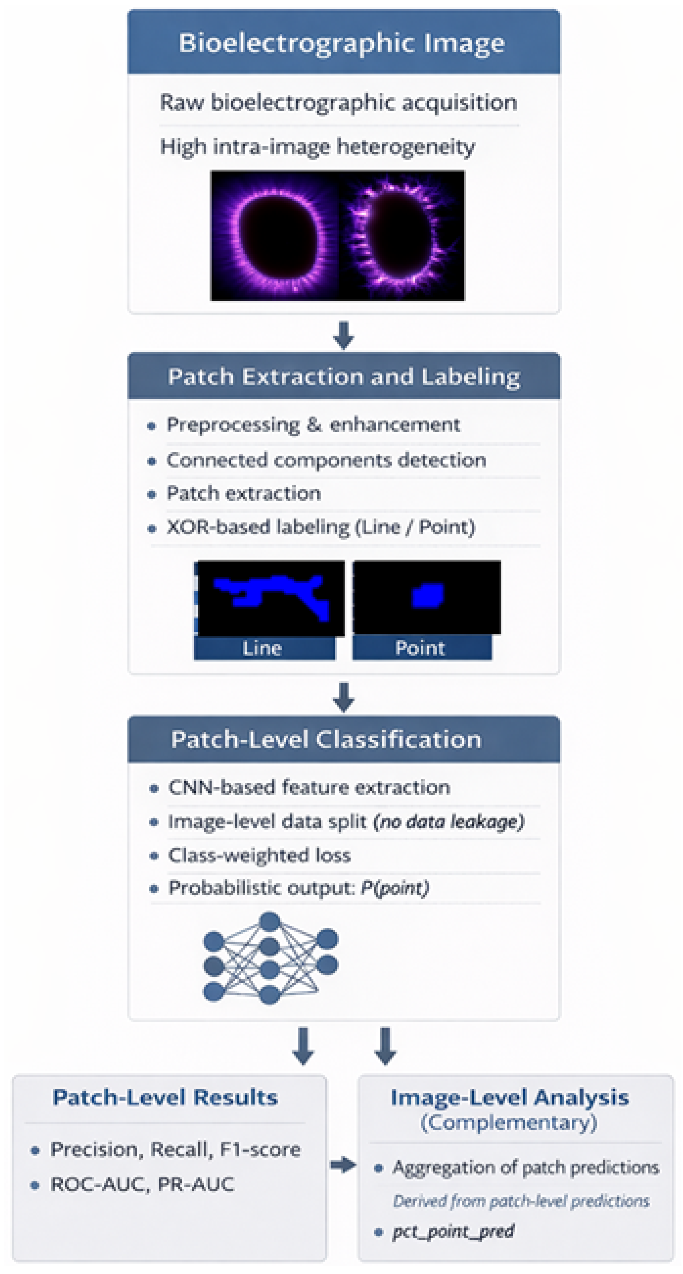
Figure 2.
Patch-level class distribution (line vs. point) after applying the XOR rule.
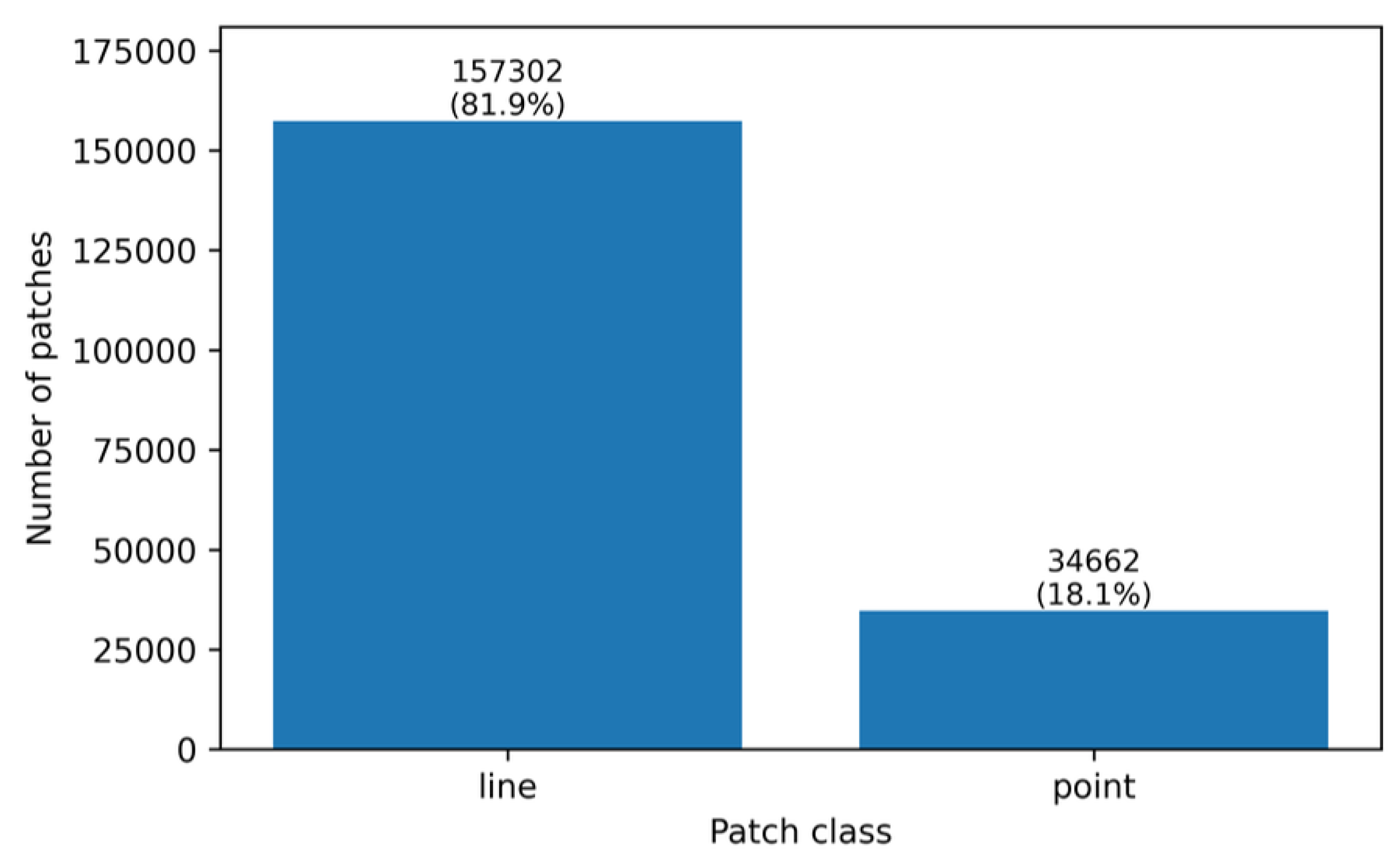
Figure 3.
Illustration of the preprocessing pipeline. From left to right: original bioelectrographic image, enhanced structural representation after preprocessing, and a combined visualization highlighting morphologically relevant structures prior to patch extraction.
Figure 3.
Illustration of the preprocessing pipeline. From left to right: original bioelectrographic image, enhanced structural representation after preprocessing, and a combined visualization highlighting morphologically relevant structures prior to patch extraction.

Figure 4.
Baseline CNN architecture used for patch-level morphological classification. The convolutional backbone is pre-trained on ImageNet and acts as a fixed feature extractor, followed by a lightweight classification head optimized for binary classification.
Figure 4.
Baseline CNN architecture used for patch-level morphological classification. The convolutional backbone is pre-trained on ImageNet and acts as a fixed feature extractor, followed by a lightweight classification head optimized for binary classification.
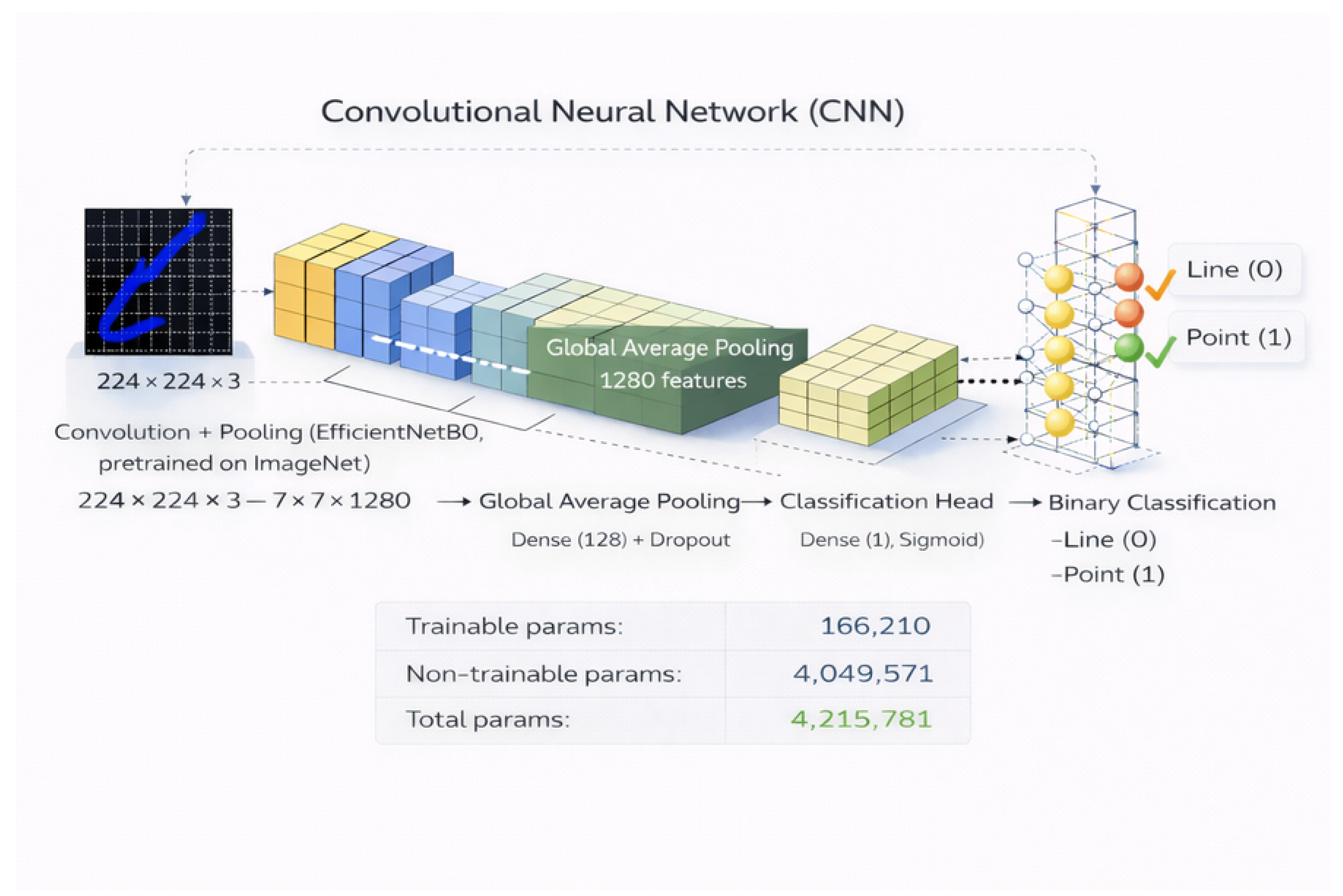
Figure 5.
Effect of image-level data splitting on the precision–recall trade-off for the point class (decision threshold = 0.50).
Figure 5.
Effect of image-level data splitting on the precision–recall trade-off for the point class (decision threshold = 0.50).
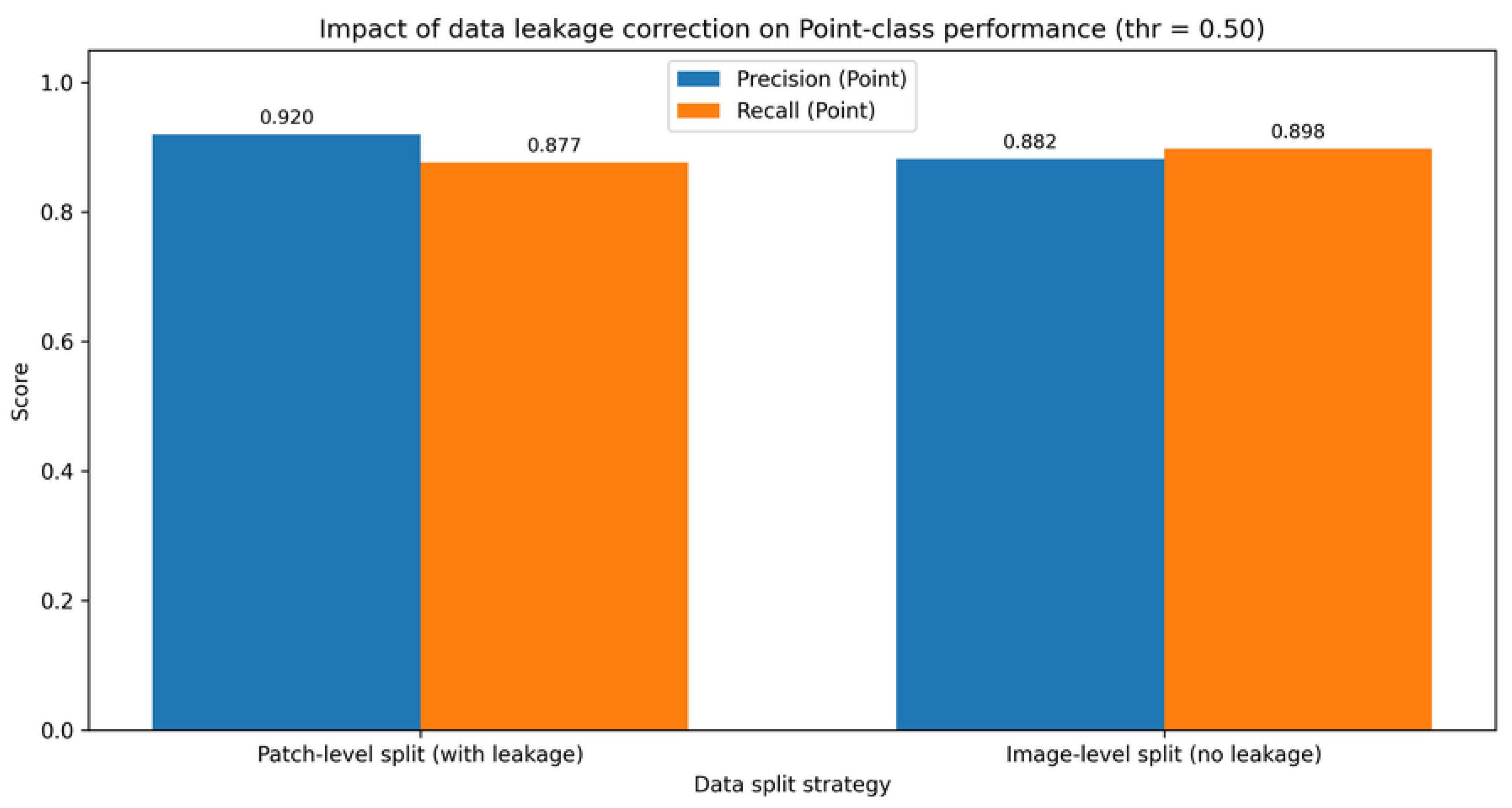
Figure 7.
ROC and Precision–Recall curves for the model trained without class weighting.
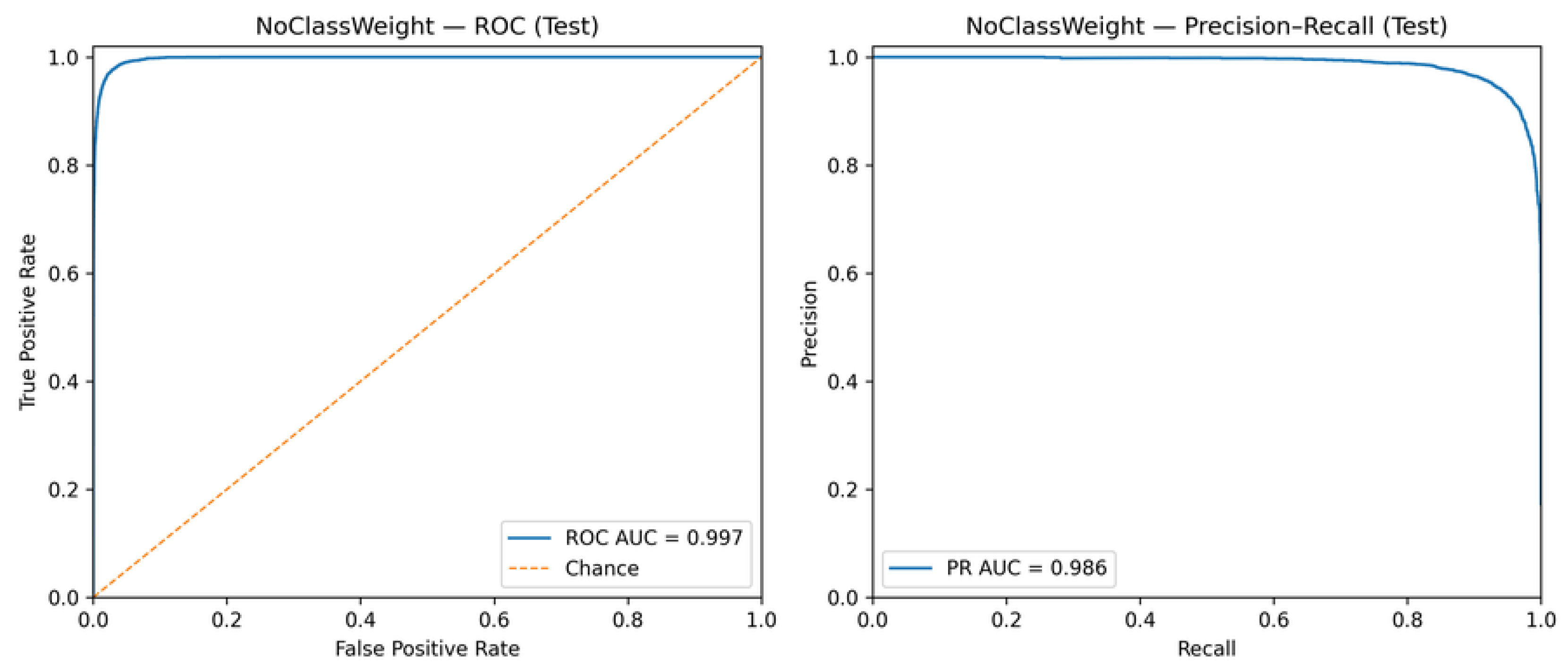
Figure 8.
ROC and Precision–Recall curves for the model trained with class weighting.
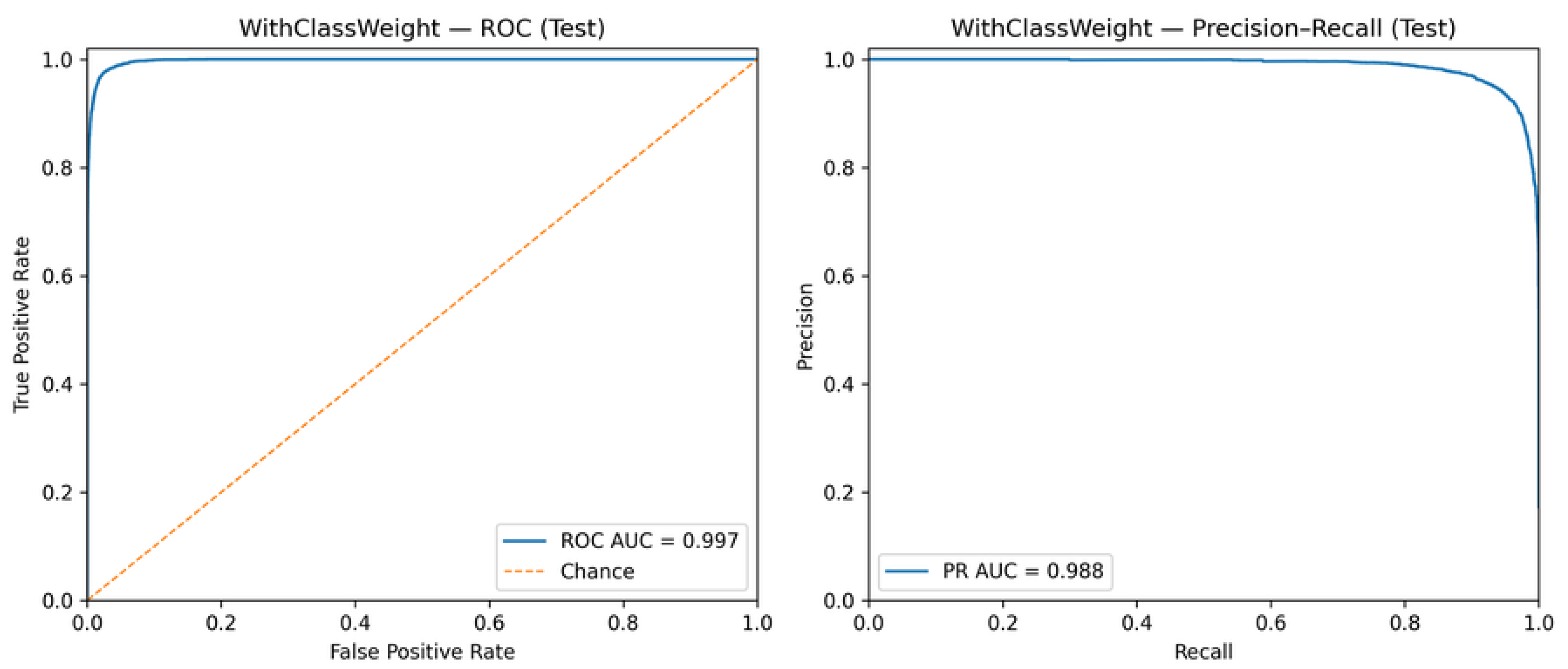
Figure 9.
Patch-level confusion matrices obtained on the test set for models trained without and with class weighting (decision threshold = 0.50).
Figure 9.
Patch-level confusion matrices obtained on the test set for models trained without and with class weighting (decision threshold = 0.50).
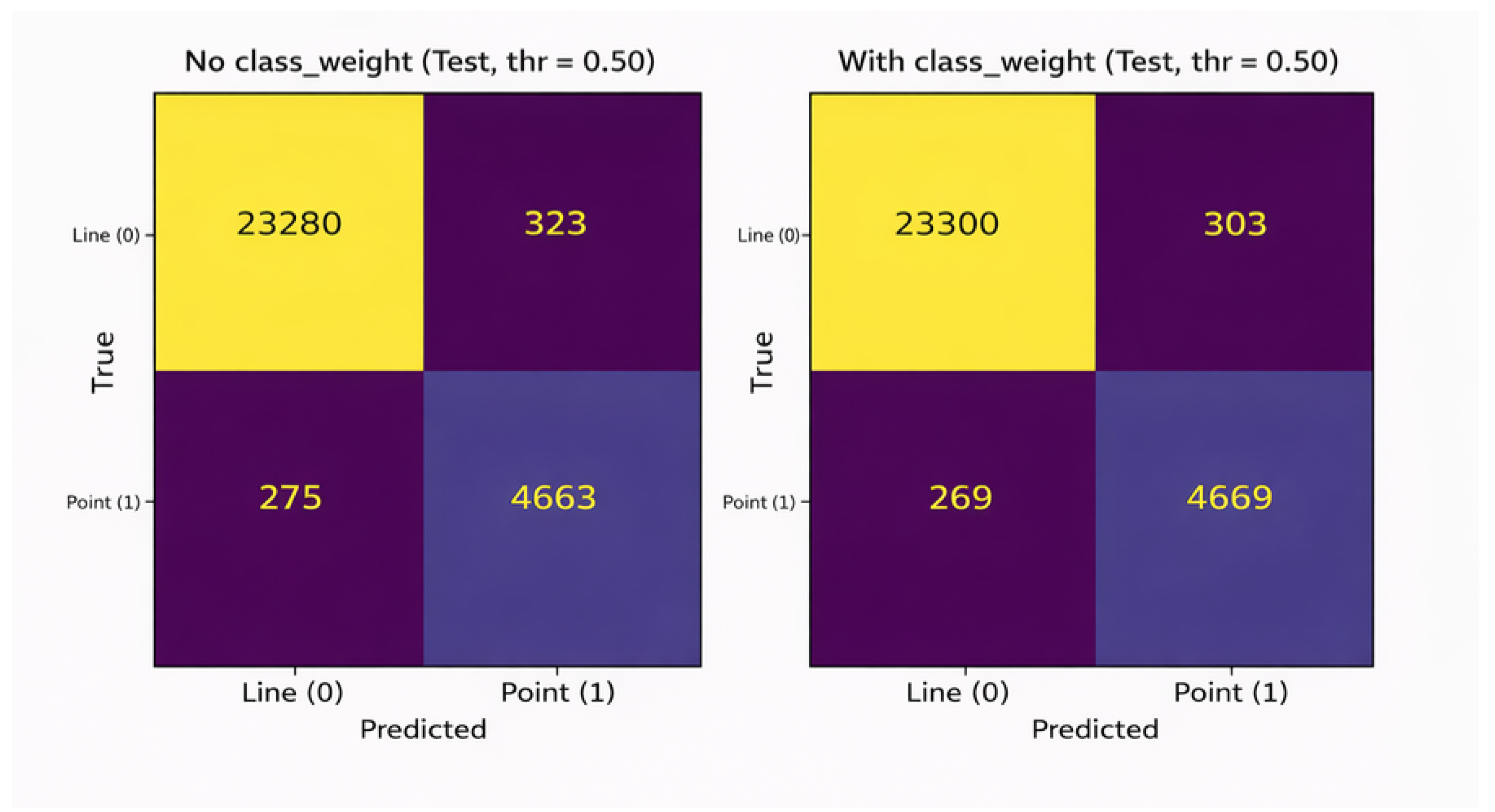
Figure 10.
Distribution of the image-level descriptor pct_point_pred across training, validation, and test sets. Similar medians and interquartile ranges indicate consistent structural composition across data splits, while the presence of outliers reflects natural inter-image variability.
Figure 10.
Distribution of the image-level descriptor pct_point_pred across training, validation, and test sets. Similar medians and interquartile ranges indicate consistent structural composition across data splits, while the presence of outliers reflects natural inter-image variability.
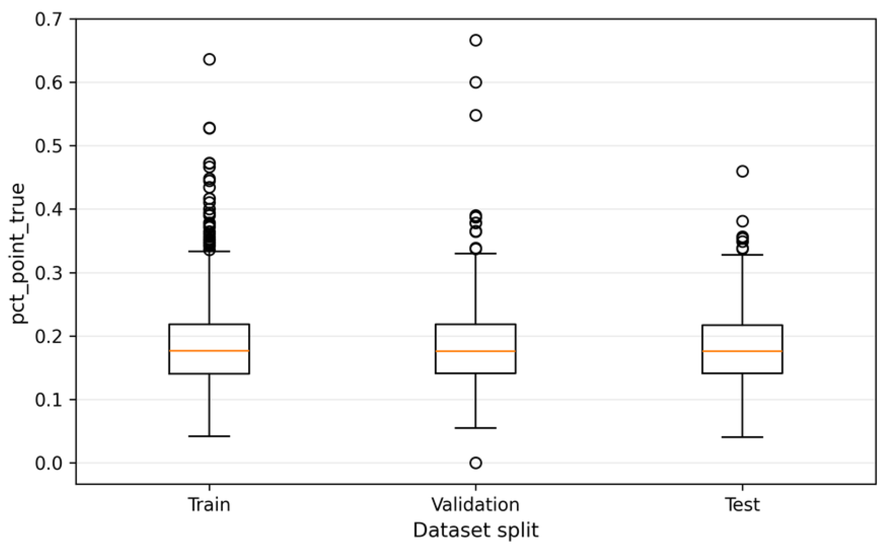
Figure 11.
Empirical distribution of the pct_point_true metric across the analyzed bioelectrographic images, highlighting substantial inter-image structural variability.
Figure 11.
Empirical distribution of the pct_point_true metric across the analyzed bioelectrographic images, highlighting substantial inter-image structural variability.
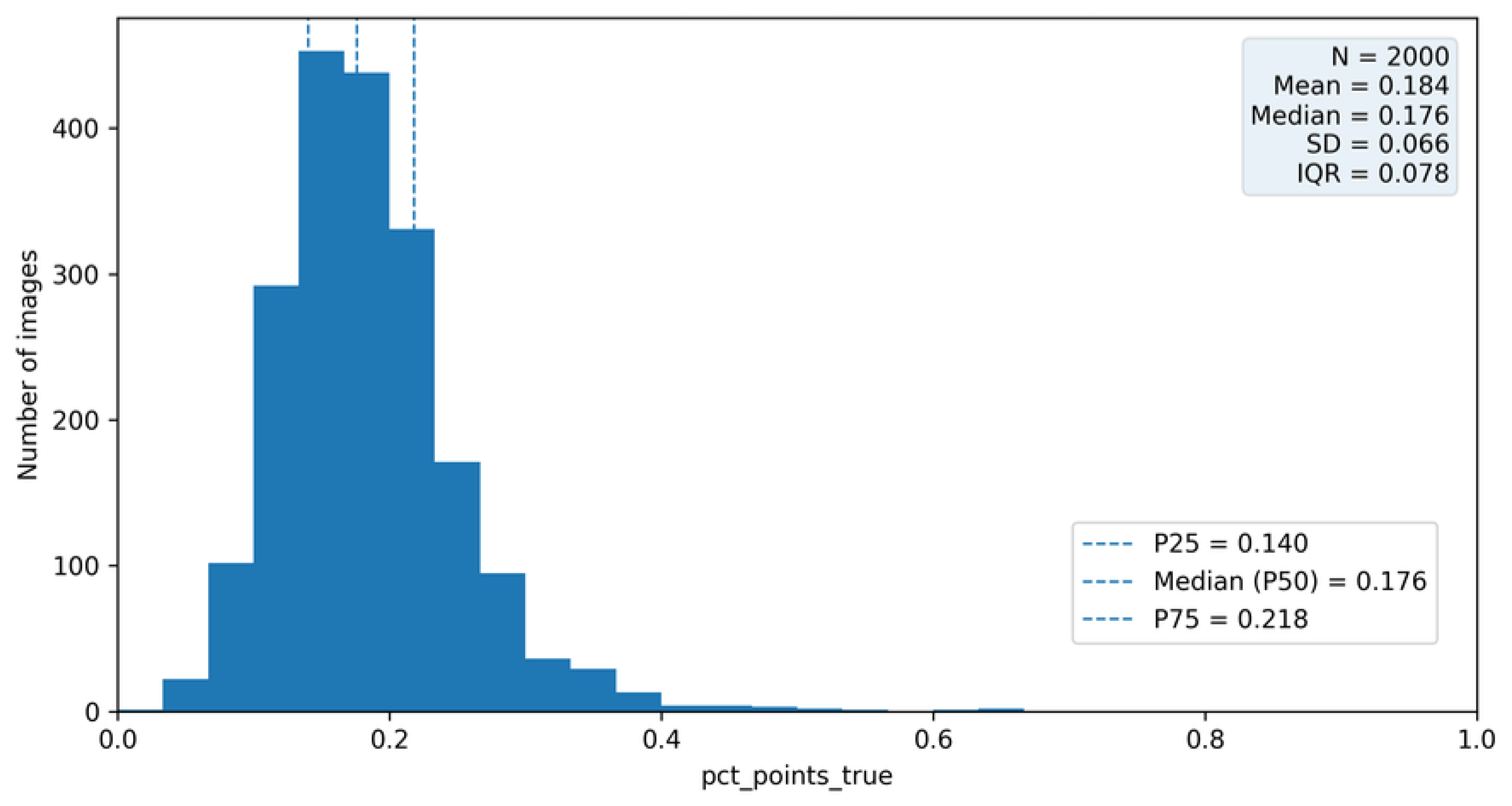
Table 1.
Summary of the analyzed dataset (image-level and patch-level volumetry).
| Statistic | Value |
|---|---|
| Number of images | 2,000 |
| Number of patches | 191,964 |
| Mean patches per image | 95.98 |
| Standard deviation | 25.13 |
| Minimum | 3 |
| 1st Quartile (Q1) | 81 |
| Median (Q2) | 97 |
| 3rd Quartile (Q3) | 112 |
| Maximum | 200 |
Table 2.
Final class distribution after applying the XOR consistency rule.
| Class | Number of patches | Percentage |
|---|---|---|
| Line | 157,302 | 81.94% |
| Point | 34,662 | 18.06% |
| Total | 191,964 | 100.00% |
Table 3.
Fixed preprocessing, patch extraction, training, and decision hyperparameters used throughout the experimental pipeline.
Table 3.
Fixed preprocessing, patch extraction, training, and decision hyperparameters used throughout the experimental pipeline.
| Stage | Parameter | Value |
|---|---|---|
| Preprocessing (edges / mask) | Ring threshold percentile () | 85 |
| Ring band width () | 18 | |
| Inner margin () | 9 | |
| Inner edge band () | 12 | |
| Gaussian blur kernel | ||
| Gaussian blur sigma | 1.3 | |
| DoG sigma1 | 0.40 | |
| DoG sigma2 | 1.90 | |
| DoG threshold percentile | 65 | |
| Morphological opening kernel | 2 | |
| Minimum blob area | 25 | |
| Resize max side (pixels) | 900 | |
| IoU acceptance threshold | 0.40 | |
| Adaptive thresholding | Target P95 | 210.0 |
| Scale factor (K) | 2.5 | |
| Threshold min / max | 65 / 72 | |
| Density factor | 1.75 | |
| Components factor | 2.0 | |
| Connectedness criterion | IoU-based filtering | |
| Binary mask generation | Enabled | |
| Patch extraction | Minimum component area | 30 |
| Padding around component | 5 | |
| CNN input and split | Input size | |
| Batch size | 32 | |
| Random seed | 42 | |
| Split strategy | Stratified by image_id | |
| Validation fraction | 0.15 | |
| Test fraction | 0.15 | |
| CNN training | Loss function | Binary cross-entropy |
| Optimizer (initial) | Adam () | |
| Optimizer (fine-tuning) | Adam () | |
| Epochs (initial) | 15 | |
| Epochs (fine-tuning) | 10 | |
| Early stopping | Enabled (patience = 5) | |
| Dropout rate | 0.2 | |
| Weight decay | Not applied | |
| Decision calibration | Output activation | Sigmoid |
| Threshold sweep | 201 values in | |
| Sweep step | 0.005 | |
| Selection criterion | Max F1 on validation set |
Table 4.
Patch-level performance comparison before and after image-level data splitting (decision threshold = 0.50).
Table 4.
Patch-level performance comparison before and after image-level data splitting (decision threshold = 0.50).
| Split strategy | Acc. | Prec. (P) | Rec. (P) | F1 (P) | Supp. (P) | FP (L→P) | FN (P→L) |
|---|---|---|---|---|---|---|---|
| Patch-level split (with leakage) | 0.9644 | 0.9202 | 0.8769 | 0.8981 | 5144 | 391 | 633 |
| Image-level split (no leakage) | 0.9600 | 0.8819 | 0.8979 | 0.8898 | 5240 | 630 | 535 |
Disclaimer/Publisher’s Note: The statements, opinions and data contained in all publications are solely those of the individual author(s) and contributor(s) and not of MDPI and/or the editor(s). MDPI and/or the editor(s) disclaim responsibility for any injury to people or property resulting from any ideas, methods, instructions or products referred to in the content. |
© 2026 by the authors. Licensee MDPI, Basel, Switzerland. This article is an open access article distributed under the terms and conditions of the Creative Commons Attribution (CC BY) license (http://creativecommons.org/licenses/by/4.0/).
Copyright: This open access article is published under a Creative Commons CC BY 4.0 license, which permit the free download, distribution, and reuse, provided that the author and preprint are cited in any reuse.


