
Submitted:
06 January 2026
Posted:
08 January 2026
You are already at the latest version
Abstract
We introduce a formal and systematic analogy between static mechanical spring networks and electrical resistor networks, establishing a one‑to‑one mathematical correspondence where spring displacements map to electric potentials, spring constants to conductances, and forces to currents. This equivalence transforms the static equilibrium equations of point-mass-spring systems into the nodal equations of resistor networks, enabling the construction of a conductance matrix that is identical in form to a mechanical stiffness matrix and coincides with the weighted graph Laplacian. We demonstrate the versatility of this framework through a series of examples from elementary series and parallel combinations to non-planar networks such as the 3D resistor cube and the Petersen graph. We show that the method provides both an intuitive mechanical interpretation of circuit concepts and a systematic, matrix-based computational algorithm for calculating equivalent resistance. The approach naturally extends to AC networks containing resistors, capacitors, and inductors, offering a unified treatment of linear networks in both DC and AC regimes. We discuss the pedagogical value of the analogy for teaching circuit theory and network analysis, as well as its connections to graph theory and computational implementation. Limitations of the method, including its restriction to linear elements and the numerical considerations of matrix inversion, are briefly discussed.
Keywords:
resistor network
; equivalent resistance
; matrix method
; graph theory
1. Introduction
Mathematical analogies between different physical systems have long been recognized as powerful tools for understanding and problem-solving in physics and engineering [1]. In electrical engineering education, analogies between mechanical and electrical systems are particularly valuable for developing intuition [2,3]. The well-known mass-spring-damper analogy to RLC circuits is a staple of systems dynamics education [4,5]. However, a formal analogy specifically between static spring networks and resistive circuits remains underdeveloped in the literature.
This paper establishes a precise mathematical correspondence between the equilibrium conditions of point masses connected by linear springs and the nodal analysis of resistor/impedance networks. The analogy provides not only an intuitive mechanical interpretation of electrical concepts but also a systematic matrix method for calculating equivalent resistance/impedance between any two nodes in a complex network.
1.0.0.1
The spring-resistor analogy builds upon the observation that Hooke’s Law for springs and Ohm’s Law for resistors share the same mathematical form,
where F is force, k is spring constant, x is displacement, I is current, G is conductance, and V is voltage. We note the directivity of both the electrical current and the mechanical force.
2. Mathematical Formalism
2.1. The Spring-Resistor Correspondence
Consider a system of N point masses connected by ideal springs obeying Hooke’s Law. For a spring connecting points i and j with spring constant , the force exerted by the mass i on the mass j through the spring is given by,
where and are the positions (abscissa) of the two endpoints relative to some reference and the unit vector is directed from point mass i to point mass j. We consider a spring with a vanishing unstretched length. For a resistor obeying Ohm’s Law, the current through a resistor from node i toward node j is,
where and are the electric potentials at the nodes, is the resistance, and is the conductance. The mathematical equivalence between Eqs. 3 and 4 establishes the fundamental analogy, summarized in Table 1. The pairing shown in Figure 1 allows a transfer of intuition about mechanical equilibrium, where forces balance and displacements propagate through a spring network to the electrical domain, where currents balance and potentials distribute through a resistor network. The identical mathematical structure, when paired with the visual analogy, reinforces the conceptual bridge between mechanics and circuit theory.
2.2. Nodal Equilibrium Equations
For a point mass m connected to several springs, static equilibrium requires,
where denotes the set of points connected to m.
For an electrical node m connected to several resistors, Kirchhoff’s Current Law gives,
2.3. The Stiffness/Conductance Matrix as Graph Laplacian
For a system with n nodes, we can write the equilibrium equations in matrix form. Let be the displacement vector (or potential vector in the electrical analogy). The equilibrium conditions yield,
where is the stiffness matrix (or conductance matrix in the electrical context) with elements:
and is the external force vector (current injection vector in the electrical context). We note that the matrix is exactly the Laplacian matrix of the underlying graph weighted by conductances [3]. This connects our method to spectral graph theory.
2.4. Equivalent Resistance Calculation: Complete Algorithm
The matrix is singular (each row sums to zero), reflecting gauge invariance of potentials (adding a constant to all potentials doesn’t change physics). To solve the system, we must ground one node (set its potential to zero). The complete algorithm is outlined as follows,
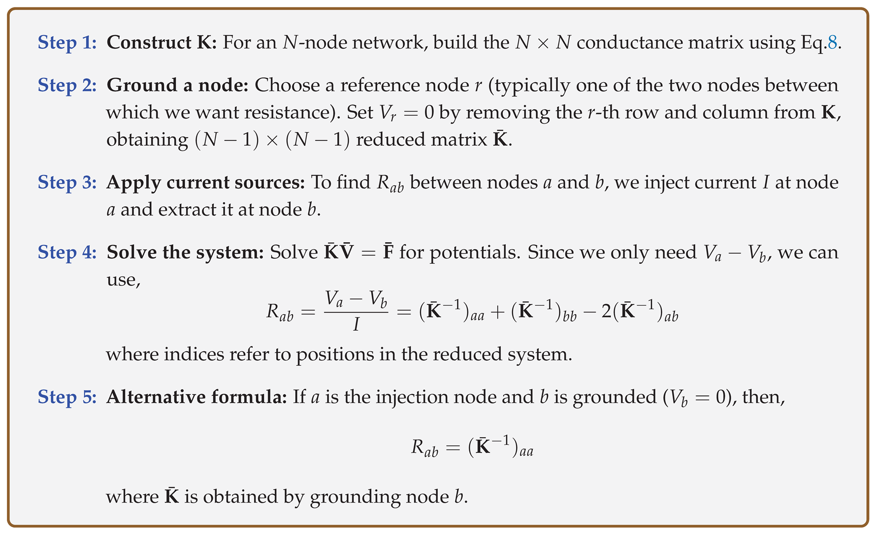
The matrix method is particularly suited to computational solution. Algorithm 1 provides pseudocode for calculating the equivalent resistance.
| Algorithm 1:Calculate Equivalent Resistance Between Two Nodes |
|
While mechanical–electrical analogies have a long history in physics education, the present work distinguishes itself in several important respects.
Traditional nodal analysis solves for node voltages given current injections, but does not inherently provide a physical interpretation of the conductance matrix. Our formulation explicitly identifies the conductance matrix as a stiffness matrix arising from Hookean springs, thereby giving a concrete mechanical meaning to each term in the matrix. This allows students to visualize current flow as force transmission and potential differences as spring displacements such perspective is absent in conventional circuit pedagogy. Furthermore, nodal analysis is indeed systematic, our formulation provides a single, consistent matrix method that works for DC resistor networks, AC networks with complex impedances, Arbitrary linear networks with dependent sources and Non-planar and high-symmetry networks, all within the same intuitive mechanical framework. Thus, the novelty lies not in discovering a new circuit solution method, but in reframing and enriching an existing method with mechanical intuition, graph-theoretical insight, and pedagogical clarity.
3. Applications
In this section we put the matrix method to the test showing its systematic resolution of different types of simple and complex electric circuits, in DC and AC regimes.
3.1. Series Resistors
Consider two resistors and in series between nodes A and C, with intermediate node B, as shown in Figure 2.
The conductance matrix is,
Ground node C (),
With current injection at A and extraction at C,
3.2. Parallel Resistors
After merging identical nodes:
Ground node B:
Thus:
3.3. Square-Cross Bridge
Consider the square-cross bridge in Figure 4 where we look for the equivalent resistance between the nodes A and D. This example shows the systematic nature of the matrix method irrespective of the complexity of the network.
The conductance matrix is given by,
For with node D grounded, we obtain after reduction to a conductance matrix,
where,
and,
which simplifies for equal resistors to,
3.4. The 3D Resistor Cube
The resistor cube in Figure 5 has 8 nodes and 12 edges. Traditional series-parallel reduction fails due to 3D symmetry. Our matrix method solves it systematically,
Step 1: Label nodes
1=A, 2=B, ..., 8=G.
Step 2: Build
Each node connects to 3 others with conductance ,
Step 3: Ground node G (node 8)
We Remove the 8th row and column.
Step 4: Solve
With current injection at A (node 1) and extraction at G,
Result:
After symbolic or numerical computation and for identical resistors ,
This matches known results from symmetry arguments, but obtained systematically.
3.5. A Non-Planar Network: The Petersen Graph
A principal strength of the formulated matrix method is its universal applicability to any connected graph structure. Formally, a graph is defined by a set of vertices V and a set of edges E connecting them [6,7]. The conductance matrix constructed in Eq. 8 is precisely the weighted Laplacian matrix of this underlying graph [8], where edge weights are given by conductances . Consequently, the algorithm for computing equivalent resistance is not limited to circuits drawn in a textbook; it provides a general solution for the resistance distance, a well-known metric in graph theory, between any two nodes in any weighted, undirected graph. This makes the method directly applicable to the analysis of celebrated and well-studied graph families such as the Petersen graph [9], complete graphs (), cycle graphs (), cubic graphs, and bipartite graphs () [10]. The formalism thus bridges circuit theory and structural graph theory, offering a computational tool for problems in network science, chemistry such as analyzing fullerene graphs [11], and beyond.
The Petersen graph in Figure 6, presents a significant challenge for traditional circuit analysis methods. With 10 nodes and 15 edges, it is non-planar, that is, cannot be drawn in a plane without edge crossings, and lacks the symmetry or series/parallel combinations to be simplified. Moreover, Delta-wye transformations introduces more complexity than simplifications. In general, each resistor has an arbitrary value, eliminating symmetry-based approaches. The matrix method provides the only systematic approach for such networks.
Matrix Method Solution
- Node labeling: Label nodes as (outer pentagon) and (inner pentagram).
-
Conductance matrix construction: The conductance matrix has,
- Diagonal elements: where
- Off-diagonal elements: if nodes i and j are connected, 0 otherwise
- Grounding: To find between nodes and , ground node ().
- Matrix reduction: Remove row and column corresponding to , obtaining matrix .
- Solution: The equivalent resistance is,
Symbolic Result:
For arbitrary resistors, the symbolic expression is extremely complex (over 100 terms even for this modest network). However, for equal resistors , symmetry yields,
Algorithm 2 solves for the equivalent resistance in an arbitrary Petersen graph.
| Algorithm 2:Solve Arbitrary Petersen Graph Resistance |
|
3.6. AC Network with RLC Elements
The network in Figure 7 contains both energy storage elements (inductor , capacitors , ) and dissipative elements (resistors , , ). In the AC regime at angular frequency , we use complex impedances,
where . The corresponding complex admittances are .
Matrix Formulation for AC:
The spring-resistor correspondence extends naturally to AC networks by replacing conductances with complex admittances,
- Complex admittance matrix: For each element between nodes i and j, compute complex admittance .
- Complex stiffness matrix: Construct with elements,
- Grounding: Ground node B, removing corresponding row/column to get .
- Complex solution: Solve where A (unit current source), for .
- Equivalent impedance: (since and ).
Symbolic Solution:
For the network in Figure 7, after grounding node B,
where rows/columns correspond to nodes A, C, D, E.
The equivalent impedance is,
The circuit has five nodes: A, B, C, D, and E. Node B is chosen as the reference (ground). The independent nodes are A, C, D, and E. The admittances of the components at angular frequency are,
The admittance matrix for nodes A, C, D, E is,
The equivalent impedance between nodes A and B is given by,
where is the submatrix obtained by deleting the first row and first column of ,
The determinants and are complex polynomials in . Their explicit expansions are,
and
These expressions provide a complete analytical solution for . For specific component values, the determinants can be evaluated numerically or symbolically to obtain the impedance as a function of frequency. The matrix method generalizes to any linear network containing resistors, capacitors, inductors, and linear dependent sources,
Complex Admittance Matrix:
For network with N nodes at frequency :
where is the complex admittance matrix, is the node voltage vector, and is the current injection vector.
Dependent Sources:
Voltage-controlled current sources (VCCS) with transconductance add terms to ,
Matrix Solution:
After grounding one node,
Equivalent Impedance:
These examples demonstrate that while traditional methods fail for complex or non-planar networks, the matrix approach provides a systematic solution. The extension to AC networks shows the method’s generality, introducing students to complex numbers and frequency-domain analysis in a unified framework.
4. Discussion and Conclusion
The spring-resistor analogy provides a powerful pedagogical bridge between mechanics and circuit theory. The matrix formulation offers a systematic computational approach for equivalent resistance that complements traditional methods [2]. Table 2 compares the matrix method to other well established circuit reduction methods, highlighting its unique position as a general-purpose, analytic and systematic technique that bridges physical intuition with mathematical formalism.
From a pedagogical perspective, the spring-resistor analogy offers several distinct advantages that make it particularly valuable for introductory circuit theory education [1]. Students who have already developed intuition about mechanical systems can leverage their understanding of forces and displacements to grasp the more abstract concepts of current flow and potential differences. This physical grounding makes electrical theory more concrete and accessible. The matrix formulation, while introducing computational complexity, provides a systematic framework that works uniformly for any resistor/impedance network, eliminating the need for the pattern recognition and cleverness often required by traditional methods. This consistency helps students develop confidence in tackling complex problems. Moreover, the analogy naturally extends to visualizing current as force flow and potential as displacement, fostering physical intuition about circuit behavior that complements the mathematical analysis. The method’s generality demonstrates the unity of mathematical approaches across disciplines, connecting circuit analysis to structural mechanics, heat transfer, and even social network theory, thereby broadening students’ appreciation for mathematical modeling [3].
However. while the matrix method introduces students to computational thinking and provides a unified analytical framework, it is important to acknowledge its inherent limitations [12]. The approach fundamentally assumes linear relationships in both domains, Ohm’s law for resistors and Hooke’s law for springs, which restricts its direct application to nonlinear circuit elements. Practical considerations include potential numerical instability in large networks, where the conductance matrix may become ill-conditioned, and the computational cost of matrix inversion, which scales as and becomes inefficient for very large networks compared to sparse solvers. Despite these constraints, the method retains substantial value for pedagogical applications and moderate-sized networks, where its systematic nature and intuitive mechanical connection provide significant educational benefits.
The method presented in this work is particularly useful for analyzing complex networks that resist solution by traditional series-parallel reduction or symmetry arguments. Future work could explore applications to random resistor networks [13], percolation theory, and the development of interactive educational tools based on this analogy, further enhancing its pedagogical impact and extending its reach to more advanced topics in network analysis and computational modeling.
References
- Burde, J.P.; Weatherby, T.S.; Kronenberger, A. An Analogical Simulation for Teaching Electric Circuits: A Rationale for Use in Lower Secondary School. Physics Education 2021, 56, 055010. [Google Scholar] [CrossRef]
- Alexander, C.K.; Sadiku, M.N.O. Fundamentals of Electric Circuits, 6th ed.; McGraw-Hill, 2017. [Google Scholar]
- Klein, D.J.; Randić, M. Resistance Distance. Journal of Mathematical Chemistry 1993, 12, 81–95. [Google Scholar] [CrossRef]
- Woodson, H.H.; Melcher, J.R. Electromechanical Dynamics; Wiley, 1968. [Google Scholar]
- Desoer, C.A.; Kuh, E.S. Basic Circuit Theory; McGraw-Hill, 1969. [Google Scholar]
- Harary, F. Graph Theory; Addison-Wesley: Reading, MA, 1969. [Google Scholar]
- Diestel, R. Graph Theory, 5th ed.; Springer: Berlin, Heidelberg, 2017. [Google Scholar]
- Merris, R. Laplacian matrices of graphs: a survey. Linear Algebra and its Applications 1994, 197-198, 143–176. [Google Scholar] [CrossRef]
- Petersen, J. Sur le théorème de Tait. L’Intermédiaire des Mathématiciens 1898, 5, 225–227. [Google Scholar]
- Bollobás, B. Modern Graph Theory; Springer: New York, NY, 1998. [Google Scholar]
- Fowler, P.W.; Manolopoulos, D.E. An Atlas of Fullerenes. International Series of Monographs on Chemistry 1995, 30. [Google Scholar]
- Golub, G.H.; Loan, C.F.V. Matrix Computations, 4th ed.; Johns Hopkins University Press, 2013. [Google Scholar]
- Kirkpatrick, S. Percolation and Conduction. Reviews of Modern Physics 1973, 45, 574–588. [Google Scholar] [CrossRef]
Figure 1.
Fundamental analogy between a single spring and a single resistor.
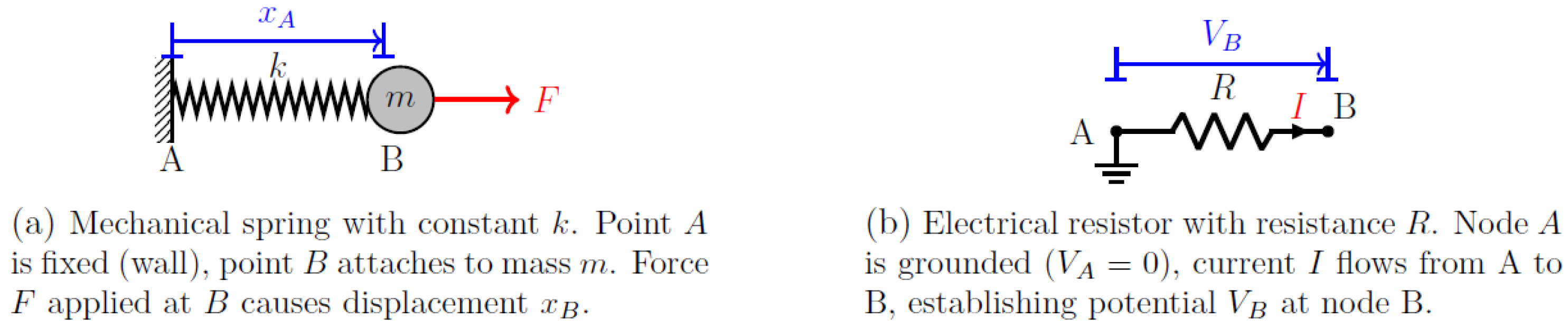
Figure 2.
Two resistors in series.
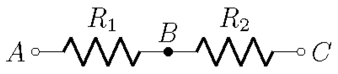
Figure 3.
Two resistors in parallel (nodes A=C and B=D are electrically same).
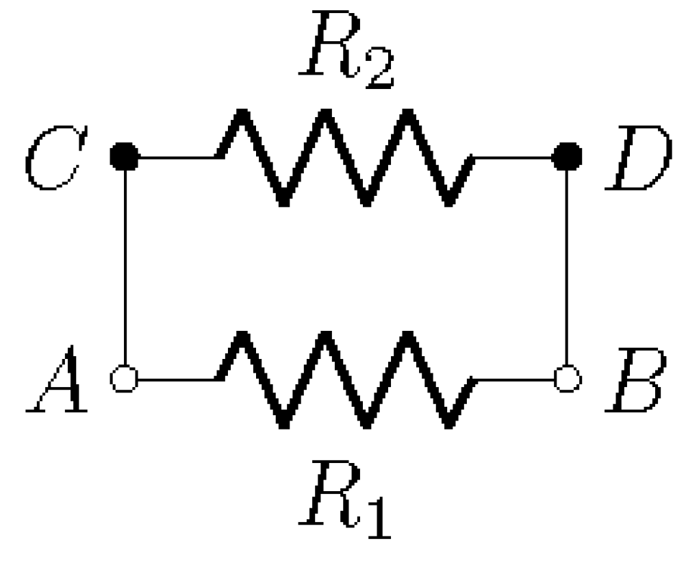
Figure 4.
Square-Cross bridge circuit.
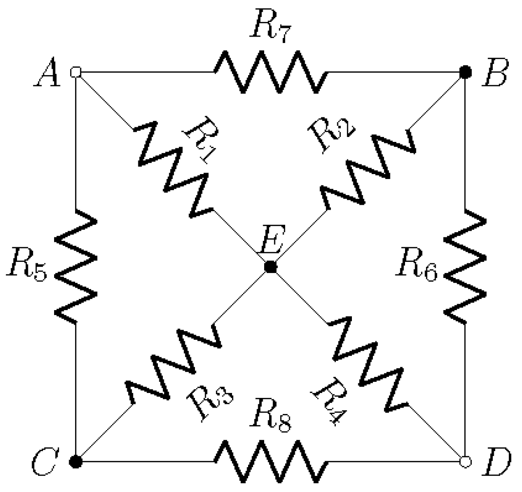
Figure 5.
3D resistor cube: 12 identical resistors R on edges of a cube. Finding (corner to opposite corner) is nontrivial with traditional methods.
Figure 5.
3D resistor cube: 12 identical resistors R on edges of a cube. Finding (corner to opposite corner) is nontrivial with traditional methods.
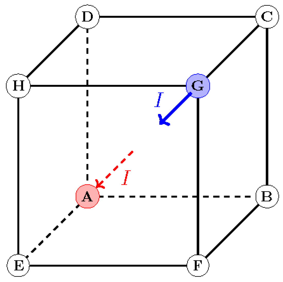
Figure 6.
Petersen graph with 10 nodes and 15 edges. This non-planar graph cannot be simplified using series-parallel or delta-wye transformations. All 15 resistors have arbitrary values .
Figure 6.
Petersen graph with 10 nodes and 15 edges. This non-planar graph cannot be simplified using series-parallel or delta-wye transformations. All 15 resistors have arbitrary values .
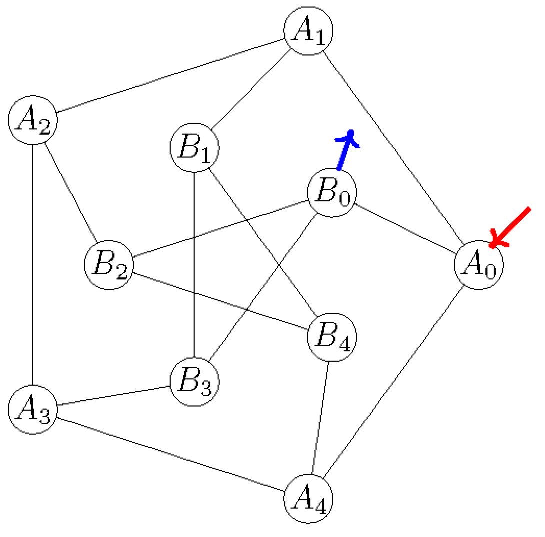
Figure 7.
AC network with resistors, inductors, and capacitors. The goal is to find the equivalent impedance between nodes A and B at angular frequency .
Figure 7.
AC network with resistors, inductors, and capacitors. The goal is to find the equivalent impedance between nodes A and B at angular frequency .
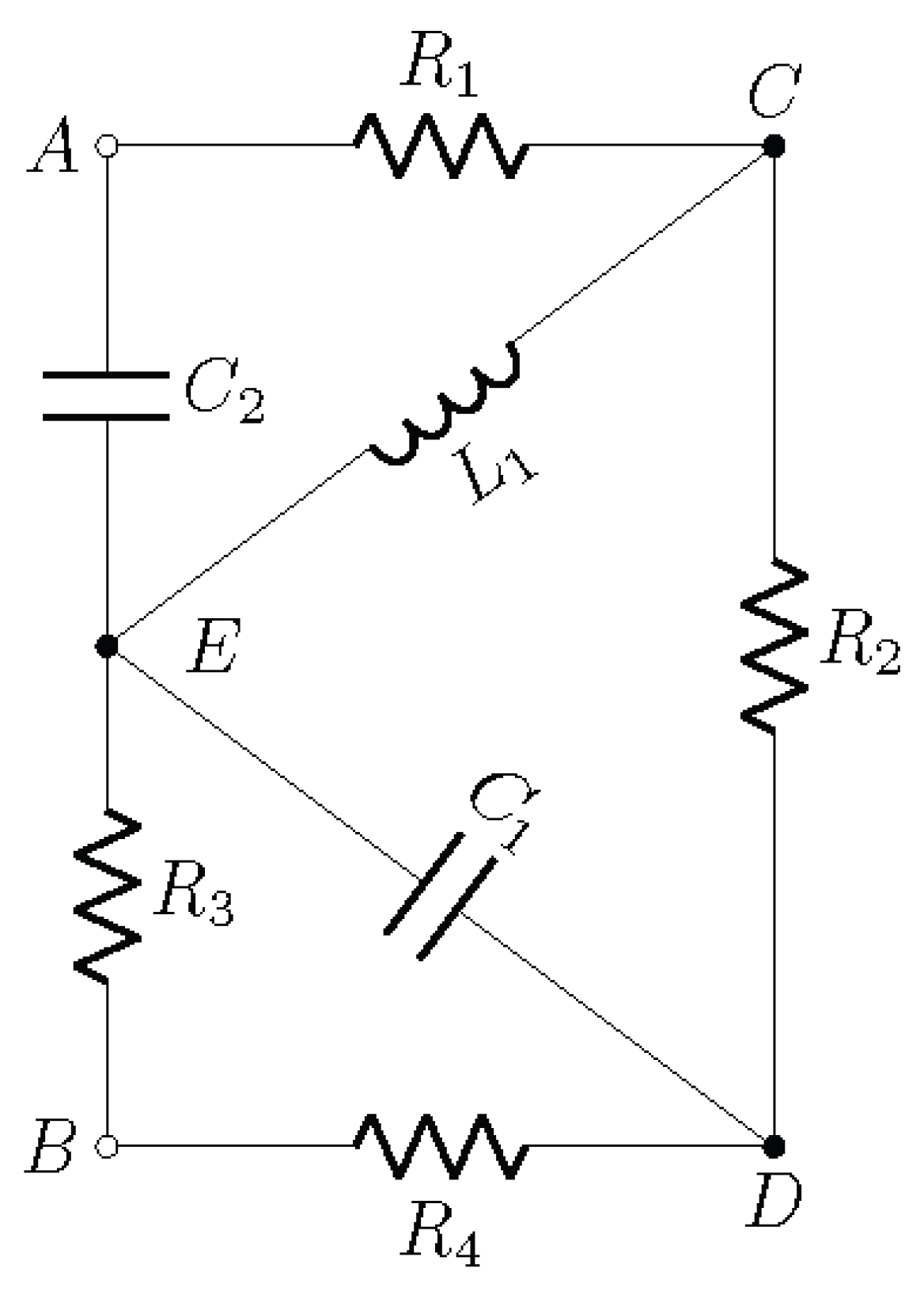

Table 1.
Correspondence between mechanical and electrical quantities
| Mechanical System (Springs) | Electrical System (Resistors) |
|---|---|
| Displacement of point i | Electric potential at node i |
| Spring constant | Conductance |
| Force in spring i-j | Current through resistor i-j |
| Point mass (node) | Circuit node |
| Static equilibrium: | Kirchhoff’s Current Law: |
| Relative displacement | Potential difference |
| External force on mass | Current injection at node |
| Stiffness matrix | Conductance matrix |
Table 2.
Comparison of resistance calculation methods
| Method | Advantages | Disadvantages |
|---|---|---|
| Series-Parallel Reduction | Intuitive, quick for simple circuits | Fails for complex networks (e.g., cube, bridges) |
| Delta-Wye Transformation | Powerful for certain symmetric circuits | Limited applicability, requires pattern recognition |
| Nodal-Mesh Analysis | Systematic, taught in standard curriculum | Requires solving linear equations manually |
| Spring-Conductance Matrix Method | Systematic for any network, connects to mechanics, computationally friendly | Requires matrix operations, singular matrix handling |
Disclaimer/Publisher’s Note: The statements, opinions and data contained in all publications are solely those of the individual author(s) and contributor(s) and not of MDPI and/or the editor(s). MDPI and/or the editor(s) disclaim responsibility for any injury to people or property resulting from any ideas, methods, instructions or products referred to in the content. |
© 2026 by the authors. Licensee MDPI, Basel, Switzerland. This article is an open access article distributed under the terms and conditions of the Creative Commons Attribution (CC BY) license (http://creativecommons.org/licenses/by/4.0/).
Copyright: This open access article is published under a Creative Commons CC BY 4.0 license, which permit the free download, distribution, and reuse, provided that the author and preprint are cited in any reuse.


