
Submitted:
06 January 2026
Posted:
07 January 2026
You are already at the latest version
Abstract
After approximately 60 years of service the 2856 MHz LINAC injector, of the Canadian Light Source (CLS), has been retired to make space for a new 3000.24 MHz LINAC injector, the frequency of which is a multiple of the 500.04 MHz CESR-B type superconductive radio frequency cavity used in the CLS storage ring. The new CLS LINAC injector has been designed and built by RI Research Instruments GmbH. The design is based on their robust S-band RF traveling wave accelerating structures technology, already serving other laboratories in the USA, Australia, Taiwan, Switzerland, and Sweden. In order to reduce cost and optimize space, the CLS has replaced its six accelerating RF structures, each 3.05 meters long, delivering 250 MeV electron beam with three 5.26 m long accelerating structures that will deliver the same beam energy. In order to do so, one RF structure is powered by one modulator-klystron and the last two RF structures receive their RF power from a second modulator-klystron that passes through a SLED system. The SLED system multiplies the peak power by a factor 5 to 6 and is then equally split to power each structure. We are reporting on the issues encountered during the commissioning of this new injector, on how we have tackled them and where the injector, compared to its technical specification, is standing today.
Keywords:
LINAC
; RF conditioning
; accelerator commissioning
1. Introduction
The new CLS "turn-key" LINAC, as a new injector for the CLS booster ring, operates at 1 Hz for beam operation and is capable of 10 Hz for Radio Frequency (RF) conditioning. A schematic overview of the LINAC beamline can be seen in Figure 1. It consists of a series of elements the first one being the 90 keV DC thermionic electron source. The electron bunches are created at cathode emitter and extracted by a pulsed and modulated grid at a frequency of 500.04 MHz. The charge and the number of electron bunches in a bunch train can be adjusted and, for operation, typically consists of ≈ 30 bunches with a charge of ≈ 100 pC per single bunch. There are five different types of RF cavities in the LINAC: A Pre-Bunching Unit (PBU), a Final Bunching Unit (FBU), three accelerating structures (ACC) and, post acceleration, an Energy Compression System (ECS) RF structure. They all operate at a frequency of 3000.24 MHz to match the harmonic of the CLS booster and storage ring frequency of 500.04 MHz [1]. Following the schematic of the beamline in Figure 1, the fifth type of RF structure is a 500.04 MHz single cell Subharmonic Pre-Buncher (SPB). It compresses each single electron bunch of the bunch train in time from the ≈ 200 ps rms at the entrance of the SPB to 10-20 ps rms at the entrance of the PBU. A single cell Pre-Bunching Unit (PBU), installed between the SPB and FBU, reduces the energy spread of the electron bunches at the entrance of the FBU. The FBU is a 14 cell traveling wave (TW) accelerator structure that compresses the electron bunches further to ≈ 10 ps rms and accelerates them to a relativistic energy of ≈ 4 MeV. Following the FBU are three identical TW accelerating structures (ACC1, ACC2, & ACC3) that bring the electron bunches to a final energy of ≈ 250 MeV. The main acceleration is provided by these three 5.26 m long 156 cell S-band TW accelerating structures with a phase advance of 120 degree per cell. In order to reach the requested beam energy, the necessary high RF accelerating electric field in ACC2 & ACC3 are being provided through one SLED (SLAC Energy Doubler) system [2].
One air cooled solenoid at the exit of the electron source and 19 subsequent water cooled solenoids surround the first 2 meters of the beamline including the SPB, PBU, FBU, and the first half meter of ACC1. The solenoids are required to keep the emittance low and to keep the non-relativistic electrons within a few mm from the optical axis of the accelerating structures. A quadrupole triplet between ACC1 and ACC2, called the Medium Energy Beam Transport (MEBT) line, keeps the beam size down to a few millimeter and quasi parallel inside ACC2 and ACC3.
Two CryoelectraTM RF amplifiers, one 500 MHz and one 3 GHz, provide the needed RF power to the SPB and PBU respectively. Two ScandiNovaTM K300 modulators with CanonTM klystrons (Canon E37302A), capable of 40 MW within 4.5 s, provide the necessary high power RF to accelerate electrons to their nominal 250 MeV. A complex waveguide network contains phase shifters and power dividers, shown in Figure 1. The phase shifters are arranged to allow for independent phasing of the cavities, while the power dividers are arranged to distribute the RF power to the various cavities in two ways. In normal mode, the RF power provided by modulator 1 is routed to reach the FBU, ACC1, and the ECS, while modulator 2 feeds ACC2 and ACC3. In recovery mode, a single modulator feeds enough power to all cavities to achieve a 180 MeV electron energy.
A number of diagnostic devices are installed along the LINAC to characterize the properties of the beam [3]. A Faraday Cup (FC) as well as an Optical Monitor (OM) are located immediately at the exit of the electron gun. A second OM is installed immediately after the SPB cavity. Another diagnostics section is located after the FBU with a Beam Position Monitor (BPM), a Wall Current Monitor (WCM), and an OM. A Fast Current Transformer (FCT), a BPM, and an OM provide diagnostics for the beam after ACC1 and ACC2. After ACC3 the total current is measured by an Integrating Current Transformer (ICT) and another FCT; a BPM and an OM locate the beam position at the exit of the LINAC prior to entering the magnetic chicane of the ECS system [4].
The design of the CLS LINAC injector is very similar to the one initially delivered by ACCEL Instruments GmbH to Paul Scherrer Institute for the Swiss Light Source [5]. The overall design has been installed and are in operation in other accelerator facilities and some of the components, like the 5 m long S-band accelerating structures, have been provided to other facilities as part of their own design. The installation of the injector was completed in early August 2024 followed by its commissioning. We are updating our previous reporting [6] regarding the RF processing and commissioning of the injector and the decision taken to come back to user operation after staying dark 9 months beyond the original plan. Commissioning experiences are usually presented in conferences and complemented within short proceedings. They are rarely presented in a long paper, like the one for SwissFEL [7]. It is even more rare to find extensive written public documentation on a commissioning failures for an operating facility. We believe that the struggle we faced may help other laboratories or companies, planning or having installed an accelerator, with their commissioning schedule in view of their intended normal operation.
2. Pre-Commissioning Work
This section describes work items that were completed prior to commencing commissioning work. It includes a brief description of the decommissioning of the old LINAC, installation of the new injector in the LINAC tunnel, as well as, work performed on various sub-components of the LINAC before and after the new LINAC installation. A final subsection describes software and tools that were developed in order for commissioning to progress.
2.1. Installation
End of May 2024, the CLS old injector was switched off and its complete disassembly started, including the removal of the modulator-klystron system feeding them that are located in a dedicated room. Over 170 individual pieces of equipment were surveyed for radiation contamination before removal, and the tunnel was cleaned, repainted, and floor resurfaced within the first two weeks of June. The rest of June focused on the installation of the two ScandiNova modulators and their electrical cabinets in the modulator room. By the end of June, the mechanical supports for the three ACCs and the MEBT were installed in the tunnel. During the month of July, the installation work continued with completion of the assembly of the three ACCs and the waveguide system that feeds RF power into them. During the month of August, all other components were installed, cabled, cooled, surveyed and the injector was put under vacuum.
2.2. Pre-Commissioning Checks
The pre-commissioning checks consist of controlling all subsystems and verifying that they perform as designed, e.g. cameras acquiring data, UHV valves closing and opening, magnet polarities being correct etc.
2.2.1. Quadrupole Triplet Verification Measurements
The MEBT, located between ACC1 and ACC2, consists mainly of steering coils and a quadrupole triplet. Following the MEBT’s arrival at the CLS and prior to installation in the LINAC tunnel, we performed a series of magnetic and survey measurements, together with beam simulations, to verify its performance. The triplet was removed from the MEBT table and each magnet tested individually; see Figure 2.
Each quadrupole’s field gradient was measured via a Hall probe, the magnetic center located via a vibrating wire [8], and the vibrating wire’s position related to fiducials via laser tracker. The measured field strengths were consistent across the magnets within 1%; field gradients at maximum magnet current (5 A) agreed with the nominal design value (4.8 T/m) within approximately 3%, which we deemed acceptable in view of the beam dynamic result.
The triplet was then reinstalled and surveyed on the MEBT table, where the quadrupoles share a common mounting rail (and have no mechanism for relative adjustment). We found the triplet’s magnetic centers were consistent within 0.23 mm and the magnetic axes parallel within 1.2 mrad. We fed the observed misalignment’s into a General Particle Tracer (GPT) [9] model of the LINAC and found they would cause only trivial steering deflections of about 0.4 mm over 14 m, easily corrected by the steering coils. Given these results, we were confident the MEBT would operate appropriately in the LINAC.
2.2.2. Magnet Polarity Tests
After installation in the LINAC tunnel, all magnets—steerers, solenoids, and quadrupoles—were tested for polarity and performance. The magnets were energized at a low current (few Amperes) and their polarity checked with a handheld magnetic field shape indicator (MagnaprobeTM Mark II). Instances of incorrect connections (open circuits, inconsistent polarity, etc.) were identified easily and resolved.
Steering magnets were disconnected during the complete system bakeout, that the RF ACC structures were subjected to, and their polarity was re-checked with the MagnaprobeTM following bakeout.
2.3. Implementation of Controls
2.3.1. Control of LLRF Waveforms
We developed a control interface to generate Low Level RF (LLRF) waveforms to send to the Cryoelettra LLRF system that controls the pulse shaping of the modulator. The waveforms include a DC pulse for modulator high voltage as well as amplitude and phase waveforms for the LLRF pulse into the klystron. The LLRF interface allows for setting the amplitude and width of the LLRF pulse to the klystron, along with timing and phase features necessary to define the pulse produced by the SLED cavity.
The LLRF waveforms are generated by a table of values defining in sequence each transition of each waveform. To reduce high frequency variations in the RF that can be generated by the instantaneous amplitude change of square pulses, we can numerically smooth the waveforms prior to sending them to the LLRF. Figure 3 shows amplitude and phase waveforms for the klystron pulse with key features annotated.
By adjusting the timestamp and shape of the appropriate rising or falling edge of the LLRF waveforms, one can manipulate the RF output waveform of the SLED. Figure 4 shows the RF forward power measured by a directional coupler at the input of ACC3 during RF conditioning on April , 2025. The observed features align well with the expected behaviour from the SLED per the LLRF settings at that time; the SLED cavity was filled for 3000 ns, the SLED phase was flipped over 100 ns, and klystron power was halted 200 ns after the start of the phase flip.
Initially the conditioning of ACC2 and ACC3 was done with a 180 degree phase flip of the RF pulse to the SLED. However, this produced an RF pulse with a sharp transition to high peak power at the time of the phase flip at the SLED output [2]. This high peak power can be the source of arcing in the accelerators. To reduce the peak power and create a more flat top compressed RF pulse at the exit of the SLED, the phase modulation of the RF input pulse was adjusted according to [10]. For our application the optimal settings were found to be a 4.5 s long RF pulse with a phase flip of 77 degree 3.3 s after the onset of the RF pulse, followed by a parabolic phase ramp to 180 degree over the next 800 ns. This produced an RF pulse with a less sharp transition to lower peak power, allowing the accelerating cavities to condition more gently. Once the accelerating cavities were conditioned to handle a certain peak power, the optimal settings were adjusted for beam operations to be a 4.5 s long RF pulse with a phase flip of 90 degree 3.3 s after the onset of the RF pulse, followed by a parabolic phase ramp to 180 degree over the next 500 ns. This produced an RF pulse with a slightly sharper transition to peak power, and by controlling the modulator output, we could maintain the same peak power. The change in phase flip settings traded conditions necessary for gentle RF conditioning, for conditions that produced a beam of higher energy and lower energy spread.
2.4. SLED Tuning
Initially the 3-dB hybrid and the two RF-cavities of the SLED were tuned during production by using a vector network analyzer (VNA) type Rhode and Schwarz ZVB8. Each separate cavity was tuned after the final brazing step by minimizing at the operating frequency. This was done by a small deformation of the bottom plate of the cavity, connected to a tuning screw. The 3-dB hybrid was tuned before the final brazing step by adjusting a tuning stub ensuring a balanced 50/50 power division and 90 degree phase difference between outputs of the hybrid at the operating frequency.
After on-site installation of the SLED system inside the high power vacuum RF waveguide network, the two RF cavities of the SLED were mechanically fine tuned. This was done by small adjustments of the tuning screws to maximize the compressed RF power at the output of the SLED. For this a flat top 4.5 RF pulse of a few kW coming from the klystron was used with a 180 degree phase inversion at 1.25 before the end of the RF pulse.
During RF conditioning of ACC2 and ACC3 the increase in RF power from the klystron was limited to . The reflected power coming back from the SLED toward the klystron was too high and interlocked the modulator to prevent the klystron from being damaged. This hardware interlock level in the modulator was set to . Depending on the setting of the waveguide phase shifter, located between klystron and SLED, reflected power peaks of up to 15 % of the klystron power were measured. Although the 3-dB hybrid and the two RF-cavities of the SLED were tuned during production, onsite mechanical fine tuning of the cavities was required to reduce the reflected power. On distance motorized tuning of the cavities was unfortunately not available. Instead of physically removing the RF-cavities and retuning them separately by minimizing at the operating frequency, it was chosen to retune the cavities by interdependently adjusting the temperatures of the SLED RF-cavities. By using the temperature tuning technique, the cavities can be tuned at high klystron power with a LLRF phase and amplitude change over time that generates the desired compressed high power RF pulse to feed ACC2 and ACC3. Another advantage is that potential excessive deformation of the cavities during mechanical tuning can be avoided.
In the current configuration the temperature of both cavities are controlled by one single temperature chiller. To be able to make small adjustments to the temperature of the cavities separately, heat tapes were wrapped around them. Each cavity was wrapped with 2 heat tapes, one on top and one at the bottom of the cavities to minimize temperature gradients over the complete volume of the cavity. One thermocouple was connected to each cavity to measure their temperature. An in-house made PLC-based bakeout controller connected to the heat tapes and thermocouples, allowed the change in temperature of the cavities to be done independently in steps and within a stability of . During high power conditioning of a few MW, scans for different cavity temperatures and settings of the phase shifter were done to determine the required temperature change of the cavities for minimal RF power reflection toward the klystron. With the optimized change in temperature for the cavities, the reflected RF power towards the klystron could be reduced to below 3%. The values of the required temperature change of the cavities were used to calculate the equivalent frequency change. This frequency change was then used to calculate the equivalent required change of the tuning screw which deforms the bottom plate of cavities. The cavities were ultimately mechanically re-tuned using these calculated values, as to void the need of using the heat tapes. Once properly mechanically tuned and according to MAX IV experience over the years, they shall be no need to retune the SLED cavities.
Given the slight imbalance of the coupling coefficients of the cavities () as measured during the factory acceptance test, a reflected power below 2 % is not expected. If this reflection would turn out to be still too high during full power operation of the klystron, the SLED cavities potentially have to be remade. This extreme case will depend on the apertures of the cavities if it cannot be mechanically fine tuned towards a more equal value of both cavities.
The overall SLED system can be de-tuned by cooling both cylinders to a lower temperature (∼) than the operating temperature (∼) using the chiller cooling/heating system. When de-tuned by temperature, in theory, the SLED cavities do not absorb power and the SLED system acts as a normal waveguide. We have observed, at the exit of the temperature de-tuned SLED system, some ripples on the flat top of the power waveform of the RF pulse (without phase inversion) coming from the klystron of . We believe that the ripples come from the imbalance of the coupling coefficients and the imperfect tuning of the cavities. CLS has used this de-tuning feature during our RF conditioning campaign for processing the ACCs, ECS and FBU RF structures to understand the influence of the SLED pulse as well as initially assessing the SLED tuning quality .
3. RF Conditioning - RF Processing
RF conditioning or RF processing of normal or superconducting RF structures, to a define targeted accelerating field, can be rather an aggressive procedure that will induce surface damages as higher electric fields on axis and on surface are achieved. The processing techniques, for normal conducting structure or superconducting cavity have been widely described in the literature since many years and modeling through controlled environment with DC techniques have been used to understand vacuum breakdown. We will not describe the onset of a vacuum breakdown (RF initiated nor DC initiated) or how damages are initiated (craters, pitting, grain movement, gas in the grain boundaries) but we will provide a set of documents as a starter for interested readers [11,12,13,14,15,16,17,18,19,20,21]. During RF conditioning, it is expected that RF breakdowns occur and RF power will be dumped in the created plasma that will create high vacuum burst and will pit the surface. Recovery past a breakdown will be the challenge for the individual responsible for conditioning the structure, not only to recover from, but to advance beyond the setback. At the end of the process, a stable accelerating field must be achieved. Stable means an accelerating field targeted that will hold during a determined time. For CLS we have targeted a time of less than 1 breakdown per 24 hours of operation and a recovery to the nominal field in less than 15 minutes. This shall be held by all RF accelerating cavities or sections independently of their resonant frequencies.
The conditioning process consists of progressively and iteratively providing more RF power to the cavities until they can sustain it without experiencing any breakdowns. During the processing, vacuum breakdowns/arcing are expected. The processing is heuristic in nature and one must build its experience while keeping in mind that patience is key. It is expected, as the processing progresses to the set goal, that less and less arcing shall occur. It is also "hoped" that after every breakdown encountered one will recover by curing the damages created by the arc through "burning" the potential source of emitter. The usual technique to process a normal conducting RF structure will use three parameters that can be modified in order to increase the overall RF energy supplied to the cavities: the pulse repetition rate, the pulse width, and the peak power.
- The pulse repetition rate controls how frequently the cavities experience RF pulses, and subsequently how frequently they can experience breakdowns that hopefully contribute to their conditioning. It is generally admitted that it is better to use a high repetition rate (50 or 60 Hz-or more if possible). At CLS our RF systems operate at maximum 10 Hz, hence our conditioning repetition rate.
- As the pulse width is increased, any imperfections or field emitters have more time under high field to experience breakdowns. By slowly increasing the pulse width, the imperfections or field emitters may be able to "evaporate", or the surface of the subsurface can rearrange itself (grain movement, gas release, electromigration [12,16,22]) which may, in case of an arc, be a lesser version of an explosive emission breakdown, hence allowing the surface to process in a safer way until reaching the desired end pulse width that is needed for beam commissioning.
- As the peak power is increased, any imperfections or field emitters, like any kind of protrusions present on the surface, will be subjected to an increased electric field strength. If the imperfections or field emitters experience too high of an electric field before they have been conditioned away, they can experience a vacuum breakdown that, instead of eating away potential field emitters, can create more "sharp" imperfections and field emitters. This type of explosive emission can potentially damage an RF structure if the repetition of this type of arcing event is high enough. By slowly increasing the peak RF power, the imperfections and field emitters may experience softer explosive emission such that the surface becomes "smoother" and can handle higher peak powers without larger breakdowns. Again, the reasons of why a surface arcs is not clear as sometimes arcs can be seen on grains without any previous damages or residual contaminants.
We hence conditioned the surface with the idea in mind that if an arc occurs we will create sharp features that can cause future damages. It is also clear that the notion of smooth, soft, and hard breakdowns are a way to describe what the processing does and how the person in charge of the RF conditioning may perceive every arcing event encountered. The surface after a vacuum breakdown never does become smooth, but rather more pitted. Surprising enough and despite the "craterization" of the surface, the damages incurred transform a mirror like surface into a moon like type of surface. If the processing is done carefully and with patience, this allows the surface to hold higher RF field strength.
Two different approaches were followed throughout the conditioning process, in both cases, one start at low power and at the smallest pulse width allowed by the RF system:
- 1.
-
Scanning pulse width:Start pulsing the cavity with low power (e.g. ) and with a short RF pulse width (i.e. ) while monitoring the vacuum levels. If the vacuum level stays below a certain threshold (e.g. ) after pulsing for a certain period of time, and the cavity does not experience any breakdowns, then the pulse width would be increased by 100 ns. The process repeats until the pulse width is increased to the final pulse width (). Once the final pulse width is reached for the given power level, the system is left pulsing in this configuration for a period of time . If the cavity did not experience any breakdowns in this time and the vacuum levels stayed below threshold, the pulse width would be reduced (typically to the starting pulse width ), the power level would be increased by a certain fraction , and the pulse width would be iteratively increased again. This process of scanning through the pulse widths for a given power level would repeat until the final power level is achieved.
- 2.
-
Scanning peak power:Start pulsing the cavity with low power (e.g. ) and with a short RF pulse width (i.e. ) while monitoring the vacuum levels. If the vacuum level stays below a certain threshold (e.g. ) after pulsing for a certain period of time and the cavity does not experience any breakdowns, then the power level would be increased by a certain fraction . The process repeats until the maximum deliverable peak power is reached . Once this final power level is reached for this given pulse width, the system would be left pulsing in this configuration for a period of time . If the cavity did not experience any breakdowns in this time and the vacuum levels stay below threshold, the power level would be reduced by an appreciable fraction . The pulse width would be increased by 100 ns, and the power level would be iteratively increased again. This process of scanning through power levels for a given pulse width would repeat until the final pulse width is achieved.
Once the procedure or algorithm is set and the variability accounted for to allow for deviations or pivoting, one can decide to process the structure manually, semi-automatically, or automatically. Depending on the individual and according to their experience, you will have a different answer of what is best. Each option has its own advantages and disadvantages. Nevertheless, even if the system is fully automated, one must look at the data (vacuum level, RF power reflected and transmitted, breakdown location, etc.) to determine if the conditioning is proceeding properly, or if one enters a risky area and whether a step back should be taken to minimize the chances to upset the surfaces.
The next question to be considered is the recovery from a breakdown, i.e. what is the procedure to be followed to bring the system back into an operational state? Or to the same value before arcing? and . Again, there are various approaches that can be taken. One may choose to reduce to a slightly lower pulse width or reduce completely to the starting point. For CLS, the shortest RF pulse is 100 ns. Alternatively, one may choose to keep the pulse width as is and reduce drastically the peak power level before restarting. Both recovery procedures were followed through the conditioning campaign depending on the circumstances and severity of the observed breakdowns. Lessons learned during the early stages of the conditioning process were applied later on, i.e not being shy to either lower the power or reducing the pulse width to almost starting point. In rare cases a combination of both reduction would be applied. Appreciating the severity of an arc and the decision of what to do is, as written earlier, an heuristic approach, however based on RF power transmitted and reflected and the vacuum level that gauges are displaying, the recovery procedure provides a guideline of what to do after the assessment of the arc severity.
Before entering the details of the conditioning, and in order to compare our S-band structure handling of the RF processing with other structures of different design or of different frequencies (C-band or X-band), we are providing in Table 1 and Table 2 a conversion between the input power seen in the cavity of our TW structure to peak field on axis or at a specific point of the surface. The conversion is calculated using the CST Studio Suite® [23]. The total acceleration that a beam shall see after 5.5 m of acceleration is calculated. It must be reminded that the magnetic field associated to the electromagnetic wave is minimal where the electric field is maximal and vice versa. The design of the cavity has to take this aspect into account due to the eddy current running on the surface due to the magnetic field variation. The RF pulse heating will induce surface stress or fatigue that can drive RF breakdowns.
3.1. Early RF Processing - 2024
After successful installation of all components in the accelerator tunnel and the RF systems in the designated modulator room, conditioning of the RF structures commenced during the month of September 2024.
During the September to December 2024 period the 3 accelerating structures (ACC1,ACC2,ACC3), the SPB and the PBU exhibited issues. Originally, it was estimated that the first three weeks of September would be dedicated and sufficient time to RF condition the whole set of accelerating structures to meet the injector technical specifications. The 5.5 m long S-band accelerating structures were conditioned with short pulses and increased power towards the klystron output of 38 MW. As the processing was ongoing the structures were conditioned in an aggressive manner e.g by not reducing the power significantly after each breakdown. The pulse length was increased quickly. As a result, the structure faced a more explosive emission RF conditioning than an evaporation RF emission, which helps smoothing the surface or smoothing out sharp edges that are the remnants of an explosive emission of a field emitter. Continuous breakdowns, mostly in ACC2, prevented any attempt of beam commissioning. In mid October 2024, it was decided to thermally de-tune the SLED cavities, as described at the end of Section 2.4, to lower the peak power directed towards ACC2 and ACC3 and feed the structure by directly coupling the RF power from the klystron to the ACC2 and ACC3 without power enhancement. Additionally, the modulators did not behave as expected and immediate support by the vendor was provided. The summary of the first months of operation and issues encountered by the modulator are shown in Figure 5. The figure shows the results achieved by the modulators over time as a measure of the power and pulse width achieved within the structures.
Furthermore, RF windows separating the vacuum in the waveguides from the vacuum in the accelerating structures that were suspected to be faulty, were removed from the system in late November 2024. Figure 6 shows the RF window separating the vacuum on ACC2 from its waveguide. It can be clearly observed a dark discoloration in the ceramic central part.
Following those modifications, conditioning was restarted and the structures reached the field gradient achieved prior to the RF windows removal but could not process further, limited by numerous arcing events in ACC2. It was then decided to lower the target power value in an attempt to achieve beam injection into the CLS booster ring with a lower beam energy than the 250 MeV specified in the call for tender. At the end of 2024, the new injector delivered a 184 MeV beam to the Booster ring, where it completed one thousand turns without the booster RF cavity on.
In parallel to the RF processing of the ACC’s, the two bunching structures, SPB and PBU, were fed independently by their own RF generators. The SPB was conditioned using its generator operating at 450 Hz but refused to condition and exhibited high vacuum spike for different settings of the two solenoids placed before and after it.
3.2. RF Processing Until April 2025
During the Christmas break, around 10 days, the LINAC was kept ready to operate. As we resumed operation, the pre-Christmas RF power values used to operate on the accelerating structures (ACC2 and ACC3) could not be reached again and both structures exhibited a higher rate of breakdowns while trying to reach the pre-Christmas operating points. We discovered that the LINAC RF waveguide system had a small vacuum leak above ACC3. As both structures are connected through the waveguides, see Figure 1, the small air leak over the 10 days downtime resulted in memory erase of the RF processing. This memory erase of RF processing or vacuum conditioning after an air vent is a known issue. This requires a full reconditioning of the system from start. In general, a recovery from an air vent does not take as long as the initial processing time (vacuum or RF conditioning).
Because of the poor performances pre-Christmas and the setback we experienced, a decision was taken to stop operation and to launch a thorough troubleshooting campaign, starting by visually inspecting all the structures. The injector was fully vented with dry Nitrogen. As expected, pitting and some discoloration were found on the input couplers of the ACC structures, see Figure 7. The amount of pitting diminished as we moved downstream of the input coupler towards the output couplers. A borescope was used to take pictures of the first four cells of the cavity. Figure 7 shows, from top to bottom, the pictures of the first, second, third and fourth irises. As it can be observed, significant pitting and discoloration was seen on the first iris. The visual evidence of arcing seems to become less obvious for subsequent irises. As it will be described in Section 4, dedicated diagnostics allowed to confirm that most of the RF breakdowns were happening near the input coupler.
The RF pick up installed at the beginning (cell 4) showed signs of pitting and it was decided to remove both RF pickups at the beginning and end of the structures (cell 156). They were replace by specially designed RF plugs to prevent RF leakage. Figure 8 shows a picture taken of the vacuum side in one of the pickups. A fiber stuck on a polymer droplet can be seen at the bottom right of the feed-through. A few other spots with mild discoloration can also be seen around the pickup, which confirmed suspicion of arcing.
The inspection of the SPB and PBU RF couplers showed some sort of copper coating on the inner piece that should have been "white" reflecting the natural color of the ceramics. The pieces were sent to RI for Sandblasting and they were reinstalled. Subsequent commissioning of the SPB, April-May 2025, showed good conditioning of the cavity including different solenoid field strengths.
The waveguides were also reconfigured to allow us to use the second modulator as a test stand to qualify every component that could be RF tested up to 38 MW and 4.5 s; RF loads, RF windows, and RF directional couplers. The RF windows, located in front of ACC1, before the SLED and in front of the ECS and FBU) were removed given their conditions, see Figure 6. Two RF windows and loads were sent to the vendor after they failed RF testing. All other components were reassembled and the full waveguides tested to our satisfaction, see Section 3.4 and Table 3.
By mid February 2025, ACC2 was the most concerning cavity as it had shown the highest breakdown rate. As ACC2 and ACC3 are vacuum connected, through their RF waveguides and through the vacuum beam pipe, recall Figure 1, any arcing in ACC2 would interlock the RF system and prevent ACC3 from reaching higher powers where it may have broken down. With ACC2 breaking down at lower power levels or shorter pulse widths than ACC3, it was not possible to judge the health of ACC3. It was decided to probe this last cavity in a stand alone mode to prove the health of ACC3 and that the RI design of the ACC structures was sound. It must be reminded that 20 similar ACC structures were delivered to MAX IV and they do operate around our targeted field gradient through a SLED system. The waveguide system was hence reconfigured to feed ACC3 only and ACC2 was disconnected from the RF system.
A bakeout of ACC3 and its temporary waveguide system was performed. Based on previous knowledge [12] a full bakeout of the injector above to remove adsorbed water was proposed prior to the injector RF conditioning started. This was disregarded for schedule reasons and a competing knowledge that a 10 Hz RF conditioning would remove the adsorbed gas. The other risk that a bakeout of the fully vacuum connected system would bring, was: the potential mechanical damages and potentially opening a leak due to a) various thermal expansion of components and b) the absence of bellows capable of absorbing such expansion. This is especially true for the copper RF waveguide system and for some of the very long (7 m) waveguides. As an example the thermal expansion for copper is calculated where L is the original length, the change in temperature and the coefficient of linear expansion for copper (16.4× /°C). Those risks, schedule and mechanical, buried the suggestion at the time. The importance of the bakeout, for 10 days, was revisited with external experts and their successes in conditioning their own RF structures or system (MAX IV and Elettra). A very precautionary approach was taken and the temperature was ramped up at a rate of per hour, up to a temperature of and of per hour, until reaching , our plateaued temperature, for a week. It should be stated that some areas, in particular those surrounding the directional couplers at the end of the cavity, were ramped to a lower maximum temperature to prevent potential damage of components only specified to and a fan was added to ensure extra cooling around those delicate components. The vacuum baseline after bakeout was improved by a factor 10. Rate of rise tests were performed in various configurations, for ACC3 alone and for the LINAC when reconnected, to control the quality of the vacuum baseline.
A careful and patient RF conditioning of ACC3 saw more progress in being able to reach higher field gradient (handling higher RF power) and longer pulse widths than it had achieved while coupled to ACC2. We confidently concluded that the design of the structures was not the cause of all of the breakdowns ACC2 had been experiencing. The following figures, Figure 9 and Figure 10, summarize the conditioning operation and issues encountered until the overall bakeout of the LINAC at the end of April 2025.
3.3. RF Processing Beyond April 2025
The whole LINAC was reassembled in May 2025. Upon the good RF conditioning results obtained after ACC3 bakeout (Figure 10), fastest RF conditioning to RF power values achieved previously, it was decided to bake the whole LINAC without the RF waveguides for a full week at . The temperature ramp-up and ramp-down was per hour. Gas analyses, with a residual gas analyzer (RGA) prior to bakeout, during ramp up (), at plateau and during ramp down () were taken. The results show a significant decrease of the water peak in the system. The RGA is located on a turbo cart attached to the LINAC vacuum system. The turbo cart was isolated from the UHV system after the ion pumps were turned on, hence the absence of an RGA at room temperature. A final note on the bakeout impact was, that although it really helped in the RF conditioning, it was not as efficient, as we could not bake the whole waveguide system and hence when the RF was poured in the waveguides and cavities, gauges and ion pumps recorded high excursion of the total pressure. This slowed down the RF processing as we had to wait for a more acceptable vacuum level (low Torr range) before increasing the RF power.
The results of the RF conditioning, at 10 Hz, to target power levels that would produce an electron beam energy of ∼180 MeV was achieved early July 2025, see Figure 11. The 180 MeV target value for this conditioning was prompted by a few factors; some contractual and some technical and are listed below:
- "Recovery Mode" target to be demonstrated as requested by the Technical Specification
- Limitation on the modulator IGBT (too low voltage rating, 1.7 kV instead of 3.3 kV) for both modulators
- Concerns regarding the health of klystron #1
Figure 11.
Klystron power output into the RF structures (FBU, ACC1, ACC2 and ACC3, with or without SLED from May to September 2025.
Figure 11.
Klystron power output into the RF structures (FBU, ACC1, ACC2 and ACC3, with or without SLED from May to September 2025.
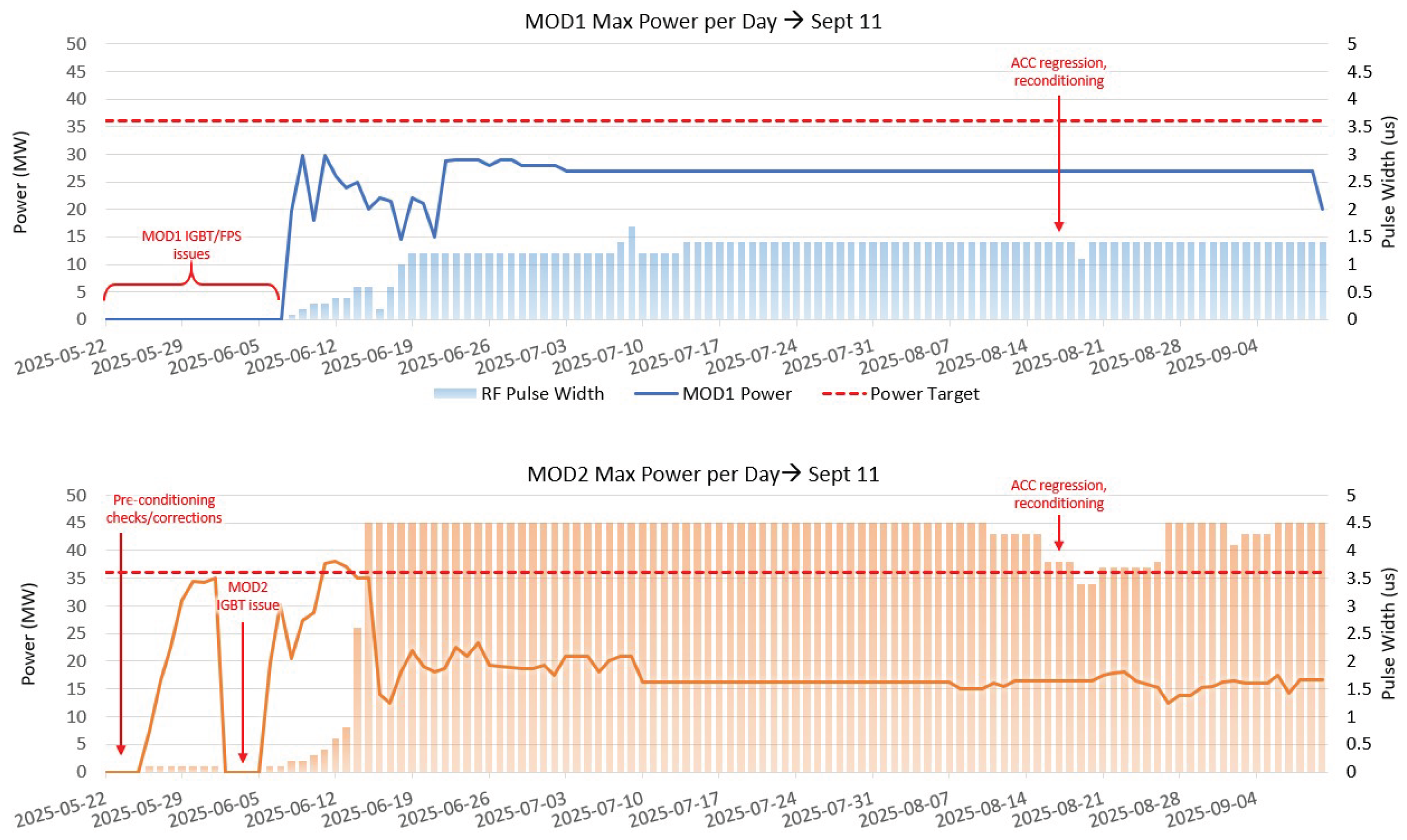
After reaching, what we considered a stable point, conditioning above the targeted equivalent of 180 MeV with a longer pulse length and holding for 12 hours at 10 Hz, was performed to provide confidence in the machine stability. We reduced the power level to the targeted goal and operated at 1 Hz to produce our first electron beam since December 2024. The team produced a quality beam from the LINAC (emittance and charge) that was captured by the Booster and sent to the Storage Ring. In just over a week, Top-Up mode at 220 mA circulating current was established.
As we were ready to provide beam for beamlines, in a more permanent fashion and after weeks of solid operation Figure 11, ACC2 suffered from a series of breakdowns. We recovered rapidly from it but a few days later one breakdown could not be recovered from without restarting RF conditioning from scratch at low power and at a shorter RF pulse length (100 ns), Figure 12. The reason of the setback is not understood. Although this came as a surprised to the RI-CLS team, this behaviour was not considered abnormal by colleagues from other laboratories.
3.4. Testing of RF Components
During several different periods of time, throughout the conditioning phase, the waveguides for the LINAC were reconfigured so one modulator could be used for testing individual RF components (windows, loads, and directional couplers) to power levels and pulse widths they would see during operation. Originally, the machine protection system (MPS) was configured in such a way that a fault detected by one of the modulator MPS would interlock the two modulators and would also stop the electron gun should there be beam.
The conditioning on each component was automated by scripting procedures that followed approach #1 (scanning pulse width) as described in the introduction to Section 3. The particular case showed in Figure 13, implemented the procedure with , a final dwell time of and a pressure threshold of 50 nTorr. The plot (Figure 13) presents the pressure values (orange line) and input power into the test stand (blue line) versus time for a period of approximately 8 hours during the spinner ACC3 RF load test. Initially the system is being pumped down until it has reached a pressure value of approximately before any input RF power is fed into the waveguide. The RF power was started near the end of February 2nd with a starting point of approximately 2.5 MW. After a small increase in power, vacuum activity was observed leading to an RF system interlocking. The RF power was restarted after a 40 minute pause to let the vacuum pressure decrease to our previous starting value. At this point, the operator started pulsing with a low 1 MW of RF power provided by the klystron with a pressure rise following a few minutes after. The RF was ramped up at a very slow rate, which was linked to vacuum pressure activity. Patience in ramping was required. At around 4 MW peak power a large vacuum event developed with pressures reaching 180 nTorr. The system under test was kept at the same RF power level until the vacuum recovered to the pressure value before the spike, 50 nTorr, and then RF conditioning was resumed.
Table 3 presents a summary of the details for all components that were tested. The duration of each test was impacted not only by equipment under test but also by the status of the machine.
4. Localizing the RF Breakdowns
As the RF conditioning did not go as planned, it was necessary to understand the location of the breakdowns. Traditionally, one can determine, with the help of 2 directional couplers, the location of the breakdown through the relative timings of the forward and reflected RF pulses [11,24]. The other method that was used successfully at SLAC in the early 2000, and then used at other labs: KEK, DESY etc. is to use a distribution of microphones [25,26,27,28].
4.1. Breakdown Localization Using the RF Signals
The edge-timing method relies on monitoring three key RF waveforms during a breakdown event, the incident (INC), transmitted (TRA), and reflected (REF) waves [24]. CLS designed a compact low-power directional coupler that fits into tight spaces and supports RF breakdown localization. It splits the RF signal so it can be sent to different devices such as RF detectors, peak power meters (for monitoring and triggering), and oscilloscopes (for viewing and recording the signal) [3]. By analyzing the temporal characteristics of these waveforms, specifically the rising edge of the Reflected (REF) signal and the falling edge of the Transmitted (TRA) signal, the breakdown position can be inferred.
Given knowledge of the physical lengths of the waveguides (WG) and accelerator (ACC) sections, along with the RF group velocity profile through each region, the breakdown time and position can be estimated within a couple of cells. The breakdown time is calculated using the relation, , where, is the breakdown time, is the time at which the reflected wave rises, is the time at which the transmitted wave falls, and denotes the RF filling time of the structure. Given the lengths of the waveguides and accelerator section and the group velocity profiles, this timing can be translated into a spatial position along the RF structure.
Figure 14 shows the three RF waveforms—INC, TRA, and REF—along with the detected edges used for breakdown localization, specifically the rising edge of the REF signal and the falling edge of the TRA signal. Figure 15 illustrates the estimated breakdown location within the accelerator structure for a representative event.
4.2. Microphone Breakdown Localization
STMicroelectonics Micro-Electro-Mechanical System (MEMS) IMP23AABSU microphones [29] were installed along the accelerator RF structures, on the waveguides and around the RF directional couplers to detect where breakdown events were occurring. The microphones are monitored at 125 kSa/s using a D-tAcq ACQ435ELF Analog Digital Converter (ADC). The data collection is triggered on the onset of a reflection, above a given threshold, seen by the directional couplers. The data acquired by the acquisition system (Figure 16) is displayed for real-time monitoring and simultaneously recorded for post-processing.
The microphones are triggered by the loss of the modulator trigger. The data is saved every time the modulator trigger is shut off, independent of the reason of why the trigger stops. In consequence, there are more data files than there are RF events. The files and their content must be filtered to identify the ones that are of interest, others can be discarded. Each data file contains the data of the event corresponding to the data registered at the time of the trigger loss, and includes the ones from the 10 triggers before. This provides non-event pulses that can be used as a baseline of a sensor response. For each file saved, the absolute maximum of the pre-final triggers were determined, the baseline is the average of all 10 maximums saved prior the loss of the trigger. To account for the noise of the sensor, the maximum amplitude is normalized against the baseline. This is shown as a solid line in Figure 17. Locations of events with a normalized amplitude over a certain value threshold, shown as the dashed line in Figure 17, are tagged with light blue markers. The sensor reacting the most to an RF event is marked with a red marker as displayed in Figure 17. It is likely the sensor the closest to where the breakdown happened.
Heatmaps from the microphone data, used in Figure 17 are displayed in Figure 18. They confirm the estimated location of the breakdowns. The heatmap plots are used for manual visual inspection to confirm the location of the RF event. In the example provided, the two figures point to an event in cell 64 of ACC3.
The data for the heatmaps is the absolute of the post-final trigger data, normalized against the absolute maximum for each microphone. So for each microphone, the black (in the color map in Figure 18), corresponding to the maximum response, value 1, is the “loudest” for that microphone. This means that the heatmap determines the “loudest” moments for each individual microphone. This adds a way to “see” the noise of the events travel through the structures. The phonon wave propagation, from cell 64, displayed in Figure 18 requires that the microphone channels are read sequentially and that the microphones are connected equally sequentially to those channels. It is not always the case that the loudest location in the amplitude plots aligned to where the noise appeared to start in the heatmaps. The heatmaps may show the noise first starting at a different location than where the loudest amplitude was. This is typically due to the different materials that make up the full accelerating structure, mainly copper but with flanges in stainless steel around the input and output couplers connecting the TW structure and the RF waveguides. RF waveguides and the RF structures are made of copper but of a different thickness. Tapping gently with a wrench, the waveguide and the RF structure produce very different sound and sound ringing. In any event(s) located close to the input couplers, the waveguides, appeared to “hear” the breakdown events the loudest regularly. Although the microphone method is simple and efficient depending on the system that is under scrutiny, more than one analysis method may be necessary to extract the appropriate information and derive the correct conclusion regarding the location of an RF Breakdown.
4.3. Overview of Breakdown Events
To develop a comprehensive understanding of the spatial distribution of RF breakdowns, both RF waveform-based and microphone-based localization techniques were systematically analyzed and compared across a series of recorded events. Two main testing periods were carried out. The first period took place between the end of March and tenth of April 2025, during which two accelerator structures (ACC1 and ACC3) were RF processed. The second period began on the ninth of June, following RF component testing and RF structure bakeout. At this stage, all three structures (ACC1, ACC2, and ACC3) were reconnected through the vacuum system and RF system for RF processing and beam commissioning over a duration of two months. A principal outcome of this study is the consistent identification of breakdowns, by both diagnostic methods, predominantly occurring near the entrance of the accelerator structures, as shown, for example in ACC2, in Figure 19. At the input coupler, or in the first cells following, the electric field is similar as the last cell as the ACC are at a constant gradient. The power however is the highest in the first cells, and as it gets absorbed by the material as it travels downstream, the structure reduces towards the end of the structure. The fact that the numerous events are located at the entrance of the structure is expected.
During the RF processing period indicated in Figure 19, the three accelerator sections (ACC1, ACC2, and ACC3) were investigated using both microphone measurements and RF waveform analysis. At this point, the accelerator team installed 32 microphones, read by the 32 ADC channels available. The microphone sensors were split between the three structures, with most microphones located at the entrance side of each RF structures.
The RF detection method records all reflected power, and triggers only when the power is above the machine protection set threshold. So not every power reflection means that the structure has been subject to arcing. In contrast, the microphone system only records events (RF breakdown probably) that causes a system interlock. Microphones react to the level of RF power dumped in the structure [27]. It may be that an arc happening at low power will not generate a sound wave in the copper that is strong enough to be easily analyzed. As a result, during structure recovery at low RF power, if reflections occur, the microphones may not record them. Therefore, statistically, the number of events detected by the RF method is usually higher than those detected by the microphones, see Figure 19 and Figure 20.
The results show that breakdown activity is concentrated near the input coupler and within the first twenty cells of the structure. As illustrated in Figure 19, the RF reflection method identifies cell 5 as the dominant hot spot, with 19 recorded events, followed by additional activity at cell 2 and a distributed region covering cells 7–14. Microphone measurements provide complementary information at the locations where sensors were installed (cells 4, 6, 8, and 18).
A discrepancy appears at cell 8, where the microphone registered a high number of events. RF localization shows that most of these events actually originated in neighboring cells rather than at cell 8 itself. Because no microphones were installed between cells 7 and 14, the sensor at cell 8 detected acoustic signals from this entire region, leading to an artificial inflation of the event count at that position.
A special case occurs at the input coupler, where 20 breakdowns were detected exclusively by microphones. RF-based localization is not applicable in this region due to wave-propagation and geometric constraints before the entrance to the accelerating structure.
Overall, after correcting for the limitations imposed by microphone placement, the RF data clearly show that cell 5 is the dominant breakdown location in ACC2, with supporting activity at cell 2 and a distributed contribution from cells 7–14, excluding the input-coupler region. Cell 4 on ACC2 used to host an RF pickup antenna, which was removed and blanked after the visual inspection around February 2025.
The number of breakdowns are monitored daily under different operating conditions - RF power levels and pulse lengths - from the klystron or the SLED. Those conditions depend on the status of the RF processing or beam commissioning. Figure 20 shows the time distribution of breakdown events observed in ACC1, ACC2, and ACC3, the daily averages of power, pulse length, and the number of events detected by both the microphone and RF methods. The direct implication of the statistic is the identification of a stable operating condition. It shows the stability of the RF source and the reaction of the structure to the RF power coming in. One can see that ACC1 and ACC3 are far more stable than ACC2. The dips in the RF power to zero may mean a maintenance period. As ACC2 and ACC3 share the same RF system - ACC2’s behaviour will drive the RF source conditions, while ACC3 stays stable with almost no reaction over time and ACC2 shows many RF events.
Figure 21 illustrates the breakdown rate for the structures between July 9 and September 16, 2025, showing trends. During this period, ACC3 stabilized at an average rate of 0.0158 events per hour.
The RF-based localization technique determines the breakdown position by comparing the arrival times of the reflected and transmitted RF signals using the known group-velocity profile inside the accelerating cells. This method is reliable within the structure, where the phase advance and group velocity vary gradually from cell to cell and produce measurable timing differences. Upstream of the input coupler, however, the RF wave travels through a short waveguide section at nearly the speed of light. In this region, the propagation time is much faster for both the phase and group velocities, and the available experimental timing resolution is insufficient to resolve the rising and falling edges of the reflected pulses with the required precision. As a result, breakdowns occurring in the coupler or upstream waveguide produce reflection times that cannot be distinguished within the timing resolution of the measurement system, and only the microphone measurements provide a reliable breakdown localization. As illustrated in Figure 17 and Figure 18, several events were unambiguously localized just upstream of the first cell, suggesting origins within the waveguide or coupler assembly.
4.4. Concluding on the Two Methods
The microphone and RF breakdown localization results were compared. The findings on the two methods discussed in this section (Section 4) confirm the complementary capabilities of the two diagnostic approaches. While RF-based timing provides accurate localization within the calibrated domain of the accelerator cells, the microphone system extends the effective detection range to include regions upstream of the structure, where RF methods are less effective. It is also noted that the spatial resolution of the microphone system varies along the structure due to the non-uniform placement of sensors, with a higher resolution near the entrance of the structure where more microphones were installed. One consideration to be reminded is that the microphone’s crude analyses were used to provide a general idea of where an event is located: beginning, middle, end of the structure and not the exact location. More advanced analysis regarding timing and installing more microphones would be needed to accurately localize vacuum breakdowns within a cell error and eventually where within one cell [27].
In summary, both diagnostic methods converge on the conclusion that breakdown events are most frequent at or near the entrance of the accelerator structure, particularly in the vicinity of the input coupler and the first few cells. This region, therefore, warrants focused investigation on quality of machining and assembly as well as opens the door for potential RF design optimization.
5. Beam Commissioning
Beam commissioning in the fall of 2024 occurred interleaved with RF conditioning during the original attempt to provide beam to the booster and ultimately to the SR. The parameters to be achieved are provided in Table 4.
Beam commissioning, even for the charges and energy of this LINAC, can be damaging to the equipment. Figure 22 shows an Yttrium Aluminium Garnet (YAG) screen that was damaged by an uncontrolled discharge of electrons from the electron source during the first round of beam commissioning. The dark current coming from the electron source was initially very intense and was over-focused, together with the normal beam, on the YAG. The dark current emission was adjusted at the electron source by adjusting the extraction Voltage.
The first round of beam commissioning efforts resulted in the capture by the booster ring of a 173 MeV electron beam, with up to 34 bunches of 80 pC for each bunch. The train was accelerated to 2.9 GeV extraction energy by the end of 2024. In January 2025, after a 10 day shutdown, the accelerating structures showed increased arcing. Beam commissioning activities were paused in order to investigate the causes of the breakdown in the accelerator sections, see Figure 10.
A further regression of ACC2 in August 2025, Figure 12, which we could not recover from, forced us to look for a stable operation point of the LINAC. As a consequence, the RF power in the ACCs were lowered significantly and the LINAC produced a reliable beam with an energy around 152 MeV. With such lower beam energy coming out of the injector, compared to the technical specification, a new setpoint for the booster, for capturing, accelerating the beam to 2.9 GeV and extracting it with enough charge to fill the Storage Ring, and to ensure top-up, had to be developed. During the later rounds of setting up the booster for the different energies, we adjusted the transverse tunes over the booster ramp to avoid resonances and improve capture efficiency, though there were still losses in the range of 50% during the first 100 ms of the booster ramp. In order to prepare for a future setback in RF power that the ACC can handle, a campaign of measurement to capture the beam from the injector will be developed during 2026. It shall determine the energy floor of the beam coming from the injector that can be captured by the booster for injection, with sufficient charge, in the storage ring.
5.1. Imaging of the Electron Gun Cathode
At some point in time, it was suspected that, the cathode of the electron gun may be damaged. An experiment was conducted to image the cathode of the electron gun, to verify that electrons were homogeneously emitted from the cathode surface. The second solenoid was turned off and the other 2 solenoids between the electron source and the second optical monitor (Figure 1) were adjusted so the image plane of the cathode coincides with the YAG screen of the second optical mirror. The raster of the grid, which is positioned 160 m in front of the cathode, with a wire thickness of 20 m is clearly visible in the image, indicating the cathode is being imaged, see Figure 23. The highlighted white spot are the electrons extracted at the cathode surface and the lines are formed by the grid locally blocking the electrons. The electron distributions are relatively homogeneous and was deemed good enough for further operations. The imaging of the grid can only be done when space charge effect are small. Too high space charge will blur out the grid lines. To keep space charge effects as low as possible the SPB and PBU were turned off so that there was no velocity bunching. A charge of 20 pC per bunch was used to image the cathode as GPT simulations showed that higher charges per single bunch started blurring out the grid image. To still have enough light gain from the YAG screens, a bunch train of 70 bunches was used for this measurement. Checking the cathode image on a regular base should indicate when cathode replacement is necessary.
5.2. Solenoid Tuning
Extraction of the first beam began with using the gun bias to minimize the dark current coming from the electron gun. YAG screens along the LINAC were put into the beam path, one at a time, starting closest to the gun to see the electrons as they were extracted from the gun along the beginning of the LINAC. The electron bunches at low energy are kept small in radius and quasi parallel with the solenoids. The values of solenoid currents were obtained from beam line optimizations in GPT simulations. A quadrupole triplet between Acc1 and Acc2 are used to keep the beam parallel in the higher energy section. Using steering magnets and viewing the beam on YAG screens, the beam was sent down the LINAC, through the three accelerating sections to the entrance of the Energy Compression System (ECS), the first dipole magnet of the ECS was turned on and adjusted such that the beam could be seen on a screen behind it. This first dipole can also act as a spectrometer and gave an energy estimate and energy spectrum of the electron beam.
5.3. Phase Adjustment
The initial approximate setting of the phases of the grid of the electron source and RF cavities (SPB, PBU and FBU) in the low energy part of the LINAC, can be found once the electrons can be detected by the WCM. The WCM was connected to a 3.5 GHz oscilloscope (Tektronic DPO 7354C) and shows if a single 1 ns electron bunch generated by the 500 MHz grid at the cathode is compressed in one single 3 GHz RF bucket of the FBU. For this to happen, the phases of the grid, SPB and FBU have to be close to the right settings, determined by simulation and adjusted by hand. Once the phase of the cavities in the low energy part have been found, the electron bunch becomes relativistic () and it can be sent through the accelerator till the ECS spectrometer. By turning on the RF structure one by one, the phase for maximal acceleration of each accelerating section can easily be found by looking at the energy spectrum in the ECS spectrometer.
Once this was done, optimization of the beam parameters was started. Iterative adjustments were done to optimize the RF phases between the gun, bunching units, and accelerating sections. The first accelerating section (ACC1) was used as the phase anchor and all other RF structures were adjusted with respect to it. First, the Gun phase was adjusted to minimize the energy spread observed. The phase for ACC2 and ACC3, being phase locked to each other, was then adjusted to maximize the energy gain. When achieved, the timing of the RF pulse to accelerating sections 2 and 3 was adjusted relative to the bunch trains arrival to minimize bunch-to-bunch energy spread. The overall process was iterated multiple times to maximize the beam energy and minimize the beam energy spread coming out of the LINAC. The emittance was also measured and provided extra information on the quality of the beam at the end of the LINAC.
5.4. Energy and Energy Spread Measurements
Energy measurements were done with the first dipole of the ECS, using the value the magnet was at with the 250 MeV beam from the previous LINAC. The energy was calculated with a linear extrapolation of the 250 MeV value based on what magnet value got the beam in the middle of the screen. The energy spread and stability measurements were done in the LINAC to Booster (LTB) transfer line at the first double bend achromat, where the dispersion is well known.
The energy spread and beam centroid stability are essential parameters for ensuring reliable booster capture. Figure 24 shows an energy spread measurement in a location of known dispersion; the energy spread, with a Full Width Half-Maximum (FWHM) value of 0.319%, is reasonable for capturing beam in our booster ring. In order to stabilize the energy centroid value, we added thermal insulation on the SLED cavity.
Figure 25 shows a measurement of the energy centroid stability; while there is some drift, it was acceptable for the booster.
5.5. Emittance Measurement and Comparison with the "Old" LINAC
The normalized root mean squared (RMS) emittance of the electron beam coming from the LINAC was measured at the beginning of the LTB using the quadrupole scan method [30]. The emittance of the new and old LINAC were compared.
As seen in both Figure 26 and Figure 27, the emittances of the new LINAC are much different than the old LINAC. Figure 26 compares the horizontal emittances measured, the new LINAC has a much larger horizontal normalized emittance of 58.1 mm*mrad compared to the 2.3 mm*mrad of the old LINAC. The vertical emittances, compared in Figure 27 go the other way, where the new LINAC normalized emittance, at 55.9 mm*mrad is almost half that of the old LINAC that was 88.7 mm*mrad. The difference in emittance is also linked to the quality of the beam control one had on the electron beam and optimization made to ensure capture in the booster ring. On the old linac, the beam had to be steered heavily from the gun on, which added difficulty in doing the quadrupole scan to be steering free. This is not the case with the new linac. The quality of the beam being rounder for the new injector compared to the older one also helps in its transport to the booster ring.
5.6. LINAC Temperature Stability
On Dec. 1, 2024, we observed large energy drifts, greater than 4%, correlated with changes in the RF forward power in ACC2 and ACC3. ACC2 and ACC3 are connected to the SLED, Figure 1, so it is hypothesized that the SLED shifting off resonance caused the instability. We noticed that the largest fluctuations occurred approximately every 70 minutes. The modulator room air temperature was identified as a possible source of the 70 minute oscillation. We tracked the issue to the LLRF rack in the modulator room and by forcing the rack temperature to equate the room temperature at any moment, improvement in beam stability was gained. Learning from this instability, we improved the air temperature stability in the modulator room. Note that large changes in the SLED water temperature, with a period of several minutes, was a separate but possibly interrelated source of energy drift. Insulating the SLED and adjusting the chiller regulation so that the water temperature fluctuations were less than seems to have stabilized this drift. A combination of temperature stabilization at the SLED, SLED chiller, and modulator room, as well as ensuring that the modulator/klystron operate in saturation, resulted in a large improvement in energy stability.
5.7. LINAC Frequency Variation
The LINAC RF frequency is matched to our storage ring (SR) with a nominal RF frequency of 500.04 MHz. However, over time our SR has shrunk pushing its frequency to 500.045 MHz. The LINAC frequency is adjusted by changing the temperature of all the LINAC RF structures. The nominal LINAC frequency of 500.04 MHz corresponds to a temperature of C at the RF structures. For the SR RF frequency, a C temperature change is equivalent to kHz. In order to verify that the LINAC can match the SR, we monitored the horizontal beam profile while changing the RF frequency followed by the temperature of the chillers with the ECS on. The camera (CCD0003-06) is downstream of the first dipole after the ECS, as already stated, in a location with known dispersion to measure the beam energy and the energy spread. We can measure the horizontal beam profile hence the change in energy due to the frequency shift of the structures driven by the temperature changes. Figure 28 shows the horizontal beam profile at the camera. The shift in energy, caused by the change in the RF frequency, was well compensated for by adjusting the temperature of all the structures. The LINAC performed well across the SR frequency range when both the ECS and temperature variation were used together. The LINAC exceeded the technical specification on this parameter by operating beyond the +30 kHz originally specified.
6. Summary
We hope this paper will highlight the failures one can face in any commissioning of an instrument and how realignment of decision making has allowed the team, RI and CLS, to better tackle the issues that were left unsolved after the first phase of the RF conditioning. The following will summarize the issues encountered.
To stress how long the commissioning is taking, when anything that can go wrong seems to go wrong is summarized by the overall timeline summary of the operation since September 2024 to September 2025 provided in the Figure 5, Figure 9, and Figure 11. Previous documentation quoted; Ask for two things when doing RF processing: carefulness and patience in applying one’s procedure. At CLS, and for a few reasons, we have mostly conditioned our structure manually. Finally, quoting our colleague from MAX IV regarding his lessons learned, and echoed by others: if you want to go fast, go slow.
It is clear that in the CLS case the commissioning of the LINAC did not go as smoothly as one would have hoped. We started with confidence in the overall team knowledge and experience. However, the first error was about the difference of knowledge and certitude of the CLS-RI team members, given their background and experience.
The RF conditioning strategy did not have consensus, plans laid out, including on what to do after an RF breakdown were not followed or with a too big of a deviation. Due to scheduling constraints, we started beam production in 2024, with the beam accelerated at a reduced accelerating field, compared to the technical specifications. The beam provided was on an unstable machine, as the RF system was not fully conditioned. We paid the price on the regression of the beam quality in early January 2025.
A second mistake was that we had basic functionality in our control system to start the commissioning, but not the full fledge control system that was promised/expected as a "turn-Key" machine. Although the tools present were necessary to start operation, basic Graphic User Interfaces, they were not sufficient to commission serenely. This included a semi-automatized system for RF processing. Significant efforts were required to develop viable ad-hoc solutions to diagnose problems. The lack of functioning diagnostics proved challenging. It is always an issue in a project, due to cost, to determine if a diagnostic or the quantity of a type is a nice to have or is necessary [3]. It is clear that diagnostics are mostly superfluous, until one has a problem. One shall treat diagnostic such as one decides to buy insurance. Finally, as time progressed and provided more advanced control tools, implementation of the interlocks that had been requested months ago, and availability of diagnostics - made our own reaction time and consensus on what to do, based on factual evidence, faster. The team came together on a unified strategy and held to it after collaborated discussions with colleagues from other labs that had success in their own endeavours of commissioning their own LINAC.
Out of the results obtained until December 2024, a few key decisions were taken by the commissioning team until April 2025. RF pickups were removed from all the RF ACC structures and the holes were plugged with specially made blanks. New directional couplers were installed at the end of each ACC structures before the RF loads to allow RF localization of the breakdowns. The input couplers on SPB and FBU were removed and sent to RI for sand blasting, as copper color was observed instead of the color of the expected ceramic, and reinstalled. The SPB structure was then successfully reconditioned with its own power supply at 450 Hz.
A quick program to install microphones and software to read their output through repurposed ADCs was launched. In less than 3 weeks, microphones could be read by a CLS made software. A change of strategy in our RF conditioning was operated such that a less aggressive conditioning method was used and was agreed upon by all members of the team. CLS team took point in the write up of the RF processing procedures and in their enactment, minor deviation to them were left to the appreciation of the operators on shift, while more drastic changes were either discussed by the CLS-RI team and enacted by the person in charge of the RF conditioning, or decided by the physicist in charge of the overall RF processing campaign. A bakeout to was performed on one structure followed by a less aggressive RF conditioning. Results obtained showed good improvement in term of accelerating field achieved and stability for a given power and pulse length, prompting the combined (RI and CLS) team to agree to bakeout as much of the LINAC as mechanically possible. The commissioning has resumed by slowly reconditioning the three long S-band RF structures.
The use of the RF and acoustic localization of the breakdowns were in agreement and pointed to the entrance of the structures. The visual inspection carried out in February 2025 had shown heavy pitting on the iris of the input coupler, while disappearing downstream of the input coupler, and was observed by carefully driving a borescope through the first cells of the RF structures. The visual inspection extended to the RF pick ups on all ACCs, the SPB, PBU and FBU, as well as the RF input couplers on SPB and PBU, see Figure 1 for location.
We targeted an equivalent output energy of 180 MeV from the LINAC with a breakdown rate of less that 1 breakdown per 0.1 million pulses before injecting an electron beam into the booster ring. We were expecting a possible beam commissioning by mid July 2025 for an injection in the booster, and the storage ring by end of July 2025 at the earliest. This goal was achieved until the "surprising" setback in RF performances in August 2025. New beam set points coming out of simulation and previous beam run led to a change of operating setpoint, basically bypassing the use of the PBU cavity. This is certainly important for RI for their next linac design. Today, the injector provides a reliable 152 MeV electron beam that is successfully capture by the Booster ring, accelerated and injected into the storage ring. Operation under top-up mode has been assured and users are back to the facility. Reaching the technical specification of 250 MeV electron beam at the end of the injector and other parameters, see Table 4, will require much longer time for RF processing of the actual RF structures. However, depending on their performances upon increased RF power, it may become necessary to manufacture new RF structures, with the same design or an altered design of the Input Coupler. CLS has already received a new ACC structure identical to the one installed and a new input coupler design is already in discussion for the next generation of ACC structures. Independently of the structures to be RF conditioned, they will be RF processed carefully following the now well established and accepted procedure that was developed during the past 6 months and are laid out in the document.
Acknowledgments
The authors would like to acknowledge the work by the staff of the CLS technical service department for having dismantled and installed the new LINAC from RI Research Instruments GmbH in record time. The authors also would like to acknowledge the help by the Science division staff and ex-AOD operator (P. Sharma) in volunteering to run shifts, including nights and weekends, when operators were not available. The authors are also recognizing all the efforts by the Control, Technical, and Engineering departments for their prompt assistance in all the issues encountered. The authors also thank K. Calder for her help in improving the readability of this document. The CLS and RI team acknowledges the input from colleagues from MAX IV (D. Kumbaro), CERN (W. Wuensch), SLAC (V. Dolgashev), Elettra (N. Shafqat), PSI (R. Zennaro) for their time in sharing their experience on conditioning their RF structures. A special mention to D. Kumbaro and his management for having had the pleasure to host him for a week at CLS. Numerous discussions on how to proceed supported by MAX IV evidence of success was a turning point in addressing our challenges. The Canadian Light Source received funding from the Canadian Foundation for Innovation, the Natural Science and Engineering Research Council of Canada, the University of Saskatchewan, the Canadian Institute for Health Research and the Government of Saskatchewan.
References
- CLS machine description is found under Facilities and Machine. Available online: https://www.lightsource.ca/facilities/machine.php.
- Farkas, Z.; Hogg, H.; Loew, G.; Wilson, P.B. SLED: A method of doubling SLAC’s energy. In Proceedings of the Proc. Of 9th Int. Conf. On High Energy Accelerators, SLAC, 1974, pp. 576–583.
- Batten, T.; Bree, M.; Kolmakov, I.; del Busto, E.N.; Randall, C.; Saadat, S. Beam instrumentation for the new linear accellerator at the Canadian Light Source. In Proceedings of the Proc. IBIC’25, Liverpool, UK, 2025. [Google Scholar]
- Laxdal, R. Design of an Energy Compression System for the Saskatchewan Linear Accelerator. Master’s thesis, University of Saskatchewan., 1980. [Google Scholar]
- Peiniger, M.; Piel, C.; Vogel, H.; vom Stein, P. A 100-MeV injector linac for the Swiss Light Source supplied by industry. In Proceedings of the IEEE Particle Accelerator Conference (PAC 99), 3 1999, pp. 3510–3512.
- Le Pimpec, F.; et al. Return of Expereince in the Commissioning of the New CLS LINAC Injector. In Proceedings of the Proc. IPAC2025, Taipei, Taiwan, 2025. [Google Scholar]
- Schietinger, T.; et al. Commissioning experience and beam physics measurements at the SwissFEL Injector Test Facility. Phys. Rev. Accel. Beams 2016, 19, 100702. [Google Scholar] [CrossRef]
- Temnykh, A. The use of vibrating wire technique for precise positioning of CESR Phase III super-conducting quadrupoles at room temperature. In Proceedings of the PACS2001. Proceedings of the 2001 Particle Accelerator Conference (Cat. No.01CH37268), 2001, Vol. 5, pp. 3469–3471. [CrossRef]
- General Particle Tracer - Pulsar Physics. Available online: http://www.pulsar.nl/gpt/.
- Olsson, D.; Lilja, P.; Malmgren, L. Increasing the Photon Energy for Photonuclear Experiments in MAX-lab by Phase Modulating the SLED Pulse. Technical Report LUTEDX/(TEAT-7242)/1-11/(2016) 2016.
- Adolphsen, C.; Baumgartner, W.; Jobe, K.; Le Pimpec, F.; Loewen, R.; McCormick, D.; Ross, M.; Smith, T.; Wang, J.W.; Higo, T. Processing studies of X band accelerator structures at the NLCTA. Conf. Proc. C 2001, 0106181, 478–480. [Google Scholar] [CrossRef]
- Harvey, S.E.; Le Pimpec, F.; Kirby, R.E.; Marcelja, F.; Adamson, K.; Garwin, E.L. Surface analysis of OFE copper X band accelerating structures and possible correlation to RF breakdown events. J. Vac. Sci. Technol. A 2004, 22, 1326. [Google Scholar] [CrossRef]
- Le Pimpec, F.; Ganter, R. High Voltage DC Breakdown of Technical Surfaces at PSI of Technical Surfaces at PSI, 2006. Available online: https://indico.cern.ch/event/3511/contributions/826724/attachments/694003/952903/HG2006_FLP02.pdf.
- Timkó, H.; et al. Mechanism of surface modification in the plasma surface interaction in electrical arcs. Phys. Rev. B 2010, 81, 184109. [Google Scholar] [CrossRef]
- Timkó, H.; Djurabekova, F.; Nordlund, K.; Parviainen, S.; Pohjonen, A.; Ruzibaev, A.; Samela, J.; Calatroni, S.; Santiago Kern, R.; Kovermann, J.; et al. A Review of CLIC Breakdown Studies, 2011. Available online: https://indico.cern.ch/event/132278/contributions/127875/attachments/98960/141243/Timko_CLICmeeting_08042011.pdf.
- Antoine, C.; Peauger, F.; Le Pimpec, F. Erratum to: Electromigration occurences and its effects on metallic surfaces submitted to high electromagnetic field: A novel approach to breakdown in accelerators. Nuclear Instruments and Methods in Physics Research Section A: Accelerators, Spectrometers, Detectors and Associated Equipment 2012, 670, 79–94. [Google Scholar] [CrossRef]
- Wuensch, W. A Review of Vacuum Breakdown in High-Gradient Accelerators. In Proceedings of the 2018 28th International Symposium on Discharges and Electrical Insulation in Vacuum (ISDEIV), 2018, Vol. 2, pp. 747–752. [CrossRef]
- Padamsee, H. History of gradient advances in SRF. Technical report, Cornell University, 2020,. [CrossRef]
- Padamsee, H. Superconducting Radiofrequency Technology for Accelerators: State of the Art and Emerging Trends; Willey, 2023. [Google Scholar] [CrossRef]
- Norem, J.; Insepov, Z.; Hassanein, A. An integrated approach to understanding RF vacuum arcs. Scientific Reports 2021, 11, 2361. [Google Scholar] [CrossRef] [PubMed]
- Wuensch, W.; Calatroni, S.; Djurabekova, F.; Kyritsakis, A.; Ashkenazy, Y. Fundamentals of Vacuum Breakdown in High-Field Systems. arXiv 2025. [Google Scholar] [CrossRef]
- Le Pimpec, F.; Harvey, S.; Kirby, R.; Marcelja, F. Autopsy on an RF-Processed X-band Travelling Wave Structure. arXiv 2002. [Google Scholar] [CrossRef]
- CST Studio Suite: Electromagnetic field simulation software. Available online: https://www.3ds.com/products-services/simulia/products/cst-studio-suite/.
- Rajamaki, R. Vacuum arc localization in CLIC prototype radio frequency accelerating structures. Master’s thesis, Aalto U., 2016. [Google Scholar]
- Frisch, J.; Nelson, J.L.; Le Pimpec, F.; Jobe, K.; McCormick, D.; Ross, M.C.; Smith, T. Studies of breakdown in high gradient X band accelerator structures using acoustic emission. In Proceedings of the 21st International Linear Accelerator Conference, 8 2002, pp. 790–792.
- Le Pimpec, F. Limitations on the use of acoustic sensors in RF breakdown localization. SLAC-TN-04-049, LCC-0149 2004. [CrossRef]
- Le Pimpec, F.; Frisch, J.; Jobe, K.; McCormick, D.; Nelson, J.L.; Ross, M.; Smith, T. An Acoustic Sensor System for Localizing RF Breakdown in Warm Copper Accelerating Structures. Nucl. Instrum. Meth. A 2007, 582, 345–355. [Google Scholar] [CrossRef]
- Delerue, N. Identifying high power breakdowns in accelerating structures with acoustic sensors, 2004. Available online: https://www-jlc.kek.jp/ nicolas/cband/talks/0402appi.pdf. [CrossRef]
- STMicroelectronics. Available online: https://www.st.com/en/mems-and-sensors/imp23absu.html.
- Limborg, C.; Emma, P.; Frisch, J.; Huang, Z.; Krejcik, P.; Schmerge, J. A Modified Quadscan Technique for Emittance Measurement of Space Charge Dominated Beams. Technical Report SLAC-PUB-10733, SLAC National Accelerator Laboratory, 2003. Presented at the Particle Accelerator Conference (PAC 2003), Portland, OR.
Figure 1.
Schematic overview of the positions of the different RF components, solenoids, quadrupoles, and beam diagnostics in the LINAC. This includes the RF distribution network, the electron source, RF single cell cavities, and accelerator sections. Dimensions are not to scale.
Figure 1.
Schematic overview of the positions of the different RF components, solenoids, quadrupoles, and beam diagnostics in the LINAC. This includes the RF distribution network, the electron source, RF single cell cavities, and accelerator sections. Dimensions are not to scale.
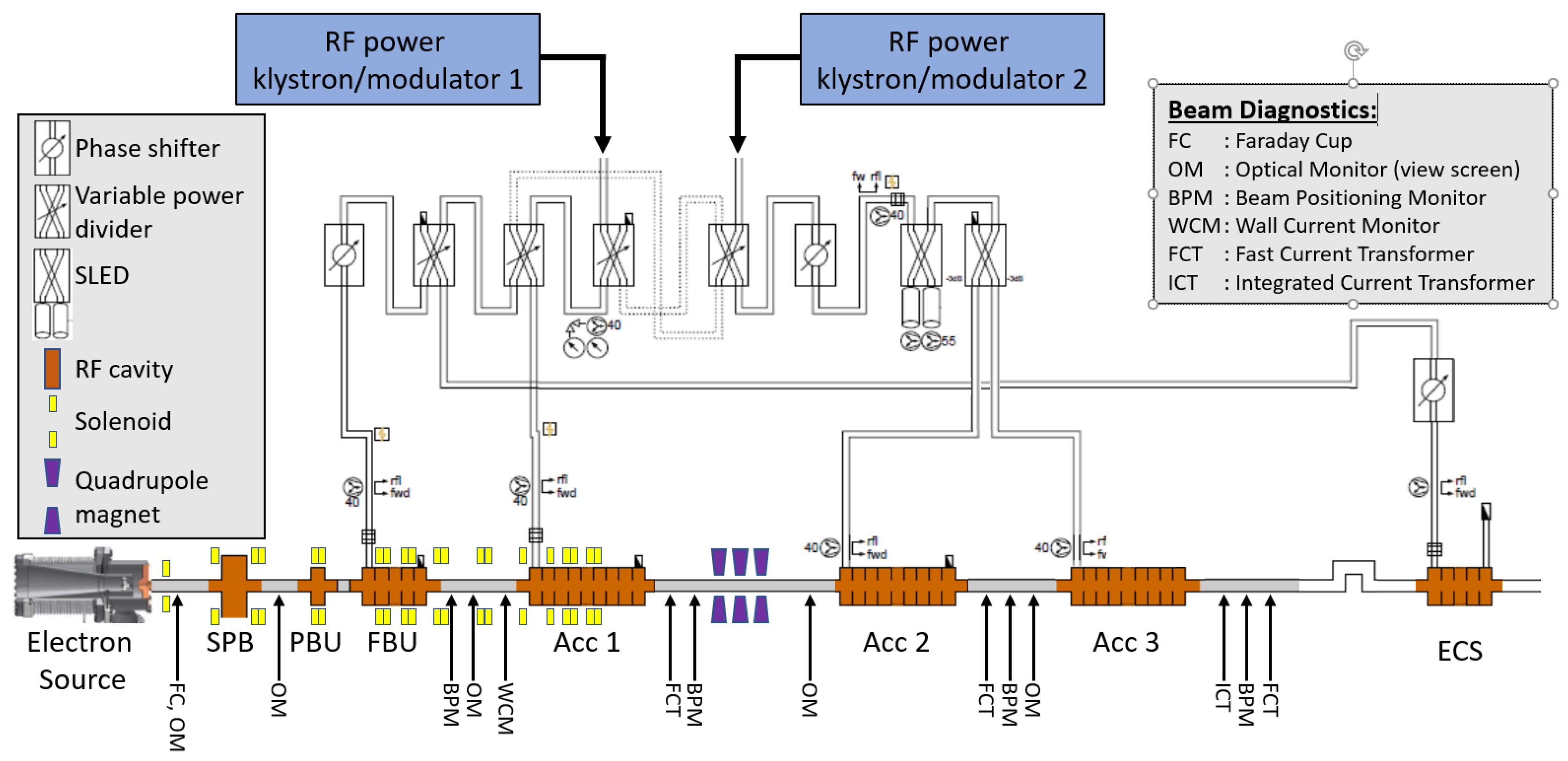
Figure 2.
One of the MEBT quadrupoles on test stand with the Hall probe and vibrating wire in place for measurement.
Figure 2.
One of the MEBT quadrupoles on test stand with the Hall probe and vibrating wire in place for measurement.
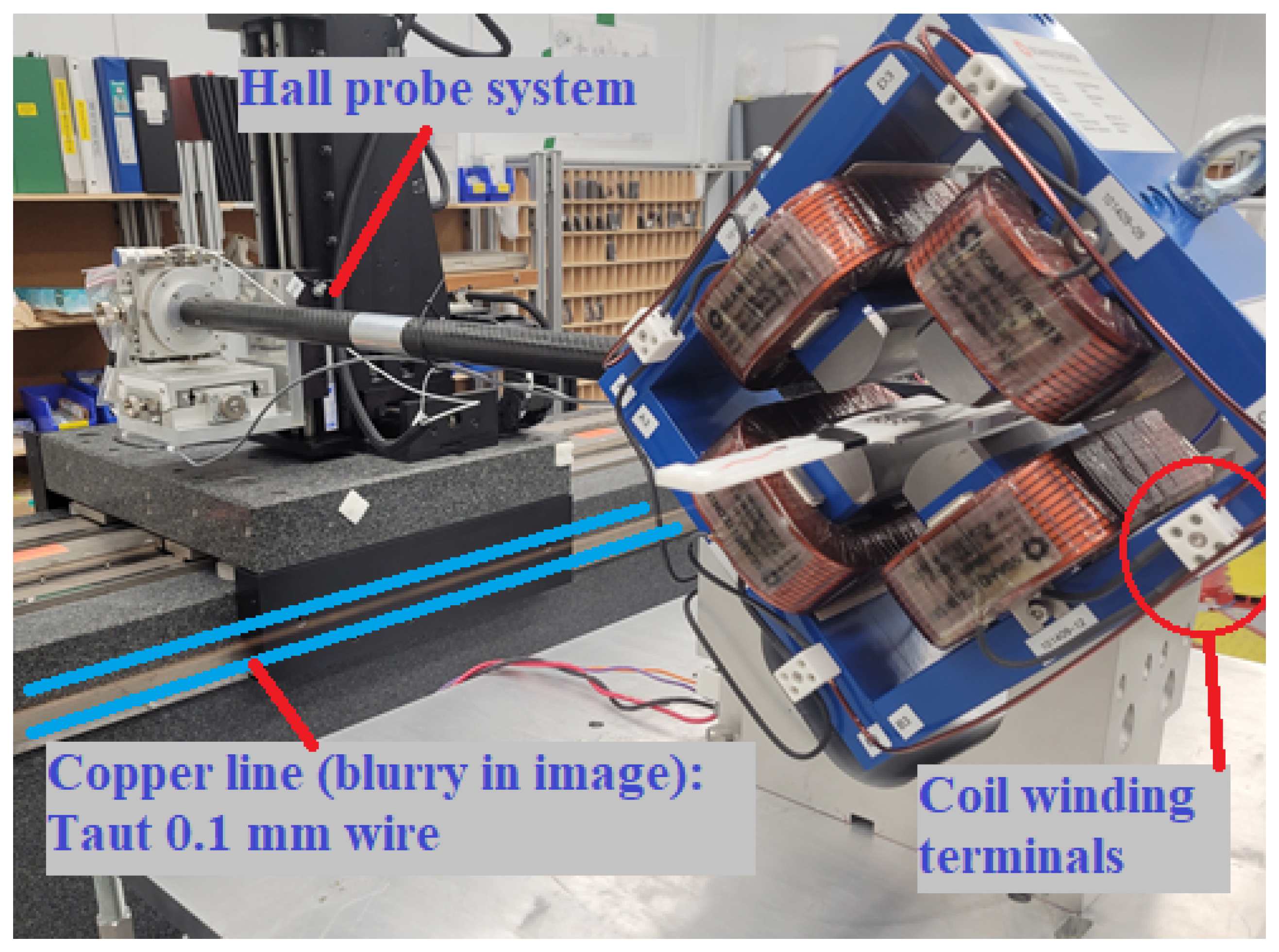
Figure 3.
A snippet of the LLRF control interface showing waveforms for klystron amplitude (above) and phase (below) with annotations to illustrate the klystron pulse width, SLED cavity filling time (time between the start of the klystrons RF pulse and the phase flip), timing of SLED phase flip, and width of SLED’d pulse (time between the phase flip and end of the klystrons RF pulse).
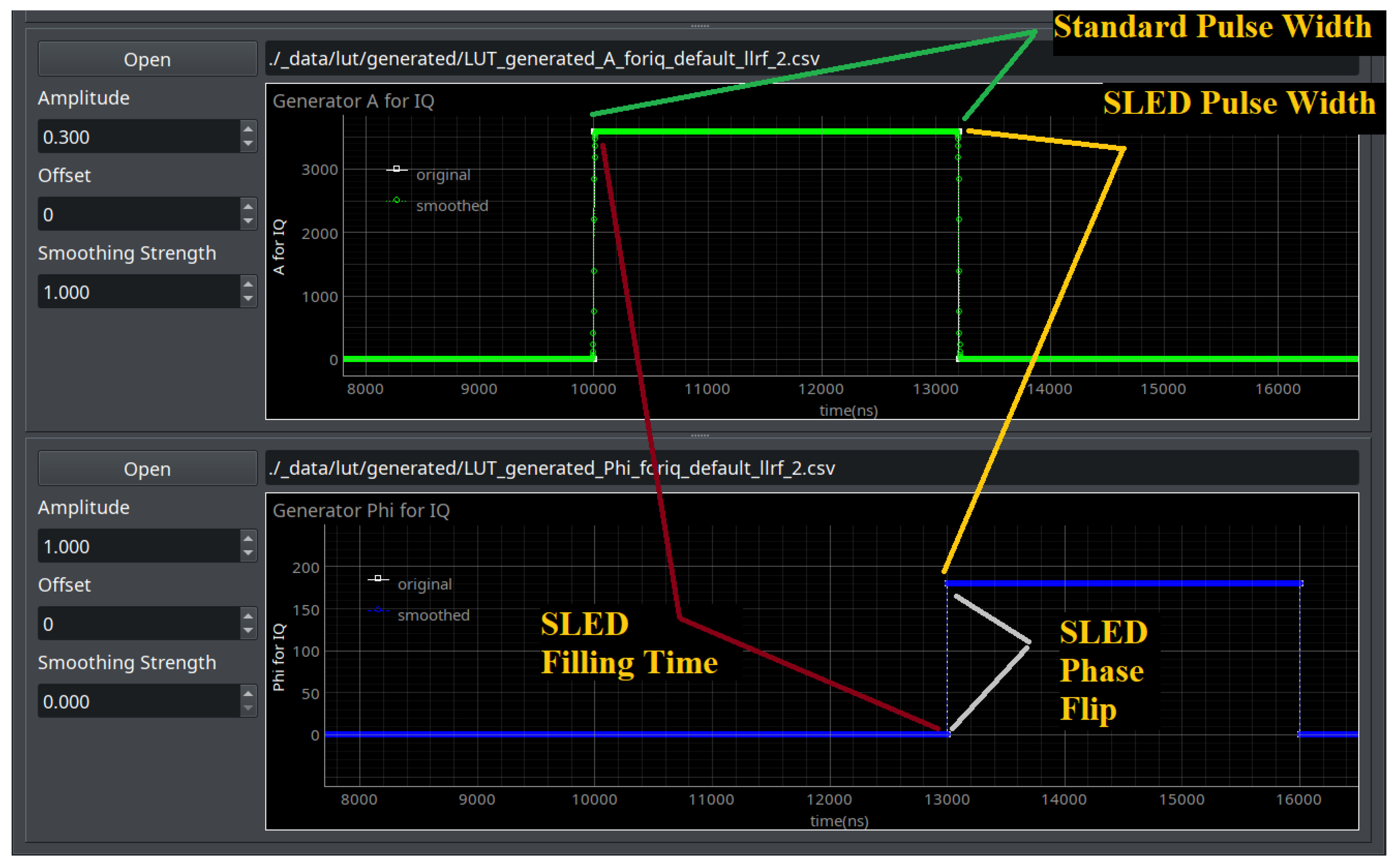
Figure 4.
Measurement of forward power from directional coupler at input of ACC3 during RF conditioning with SLED pulse.
Figure 4.
Measurement of forward power from directional coupler at input of ACC3 during RF conditioning with SLED pulse.
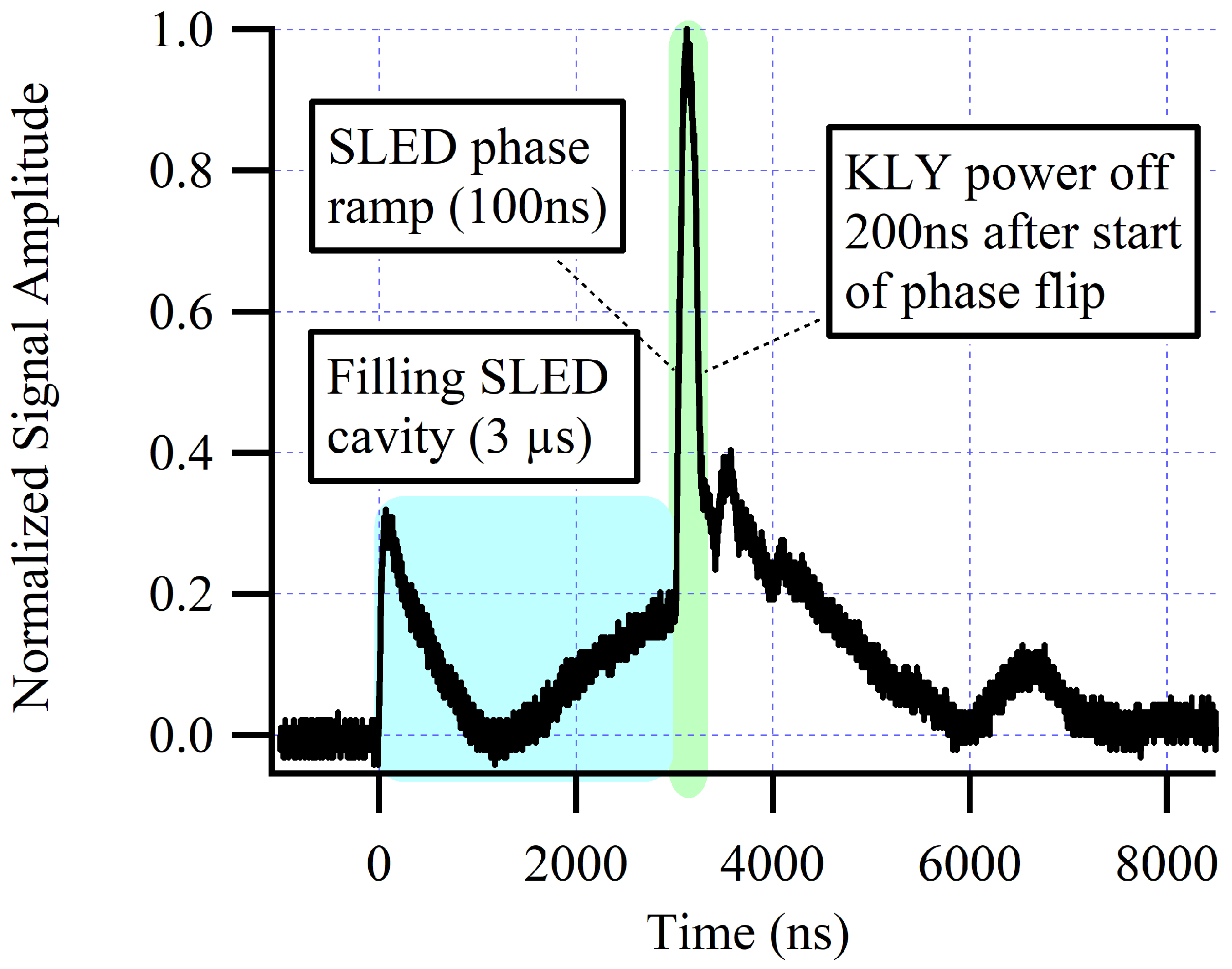
Figure 5.
Klystron power output and pulse width into the RF structures (FBU, ACC1, ACC2 and ACC3, with or without SLED until December 2024.
Figure 5.
Klystron power output and pulse width into the RF structures (FBU, ACC1, ACC2 and ACC3, with or without SLED until December 2024.
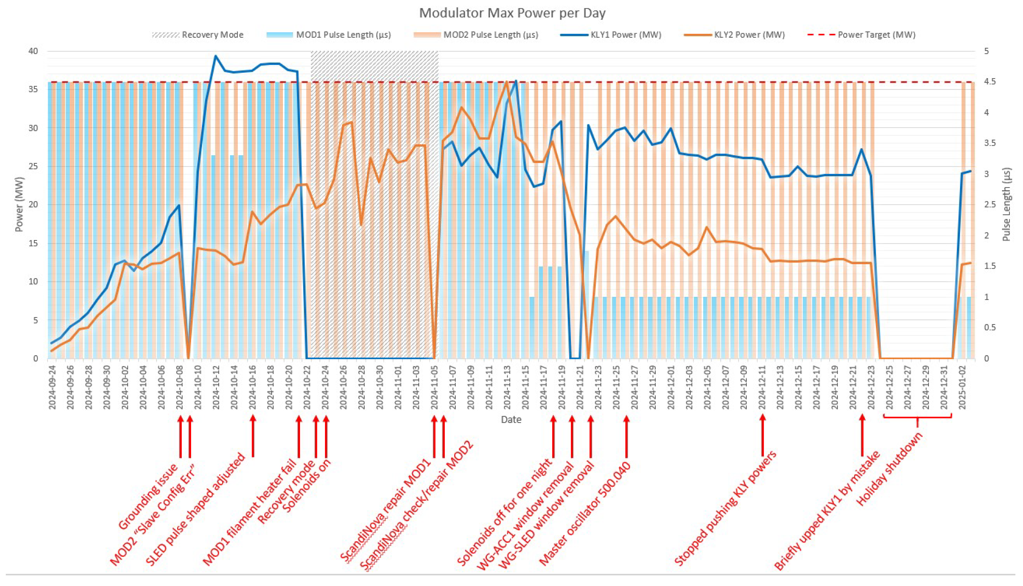
Figure 6.
Photo of the ACC2 RF Window mounted on a CF flange.
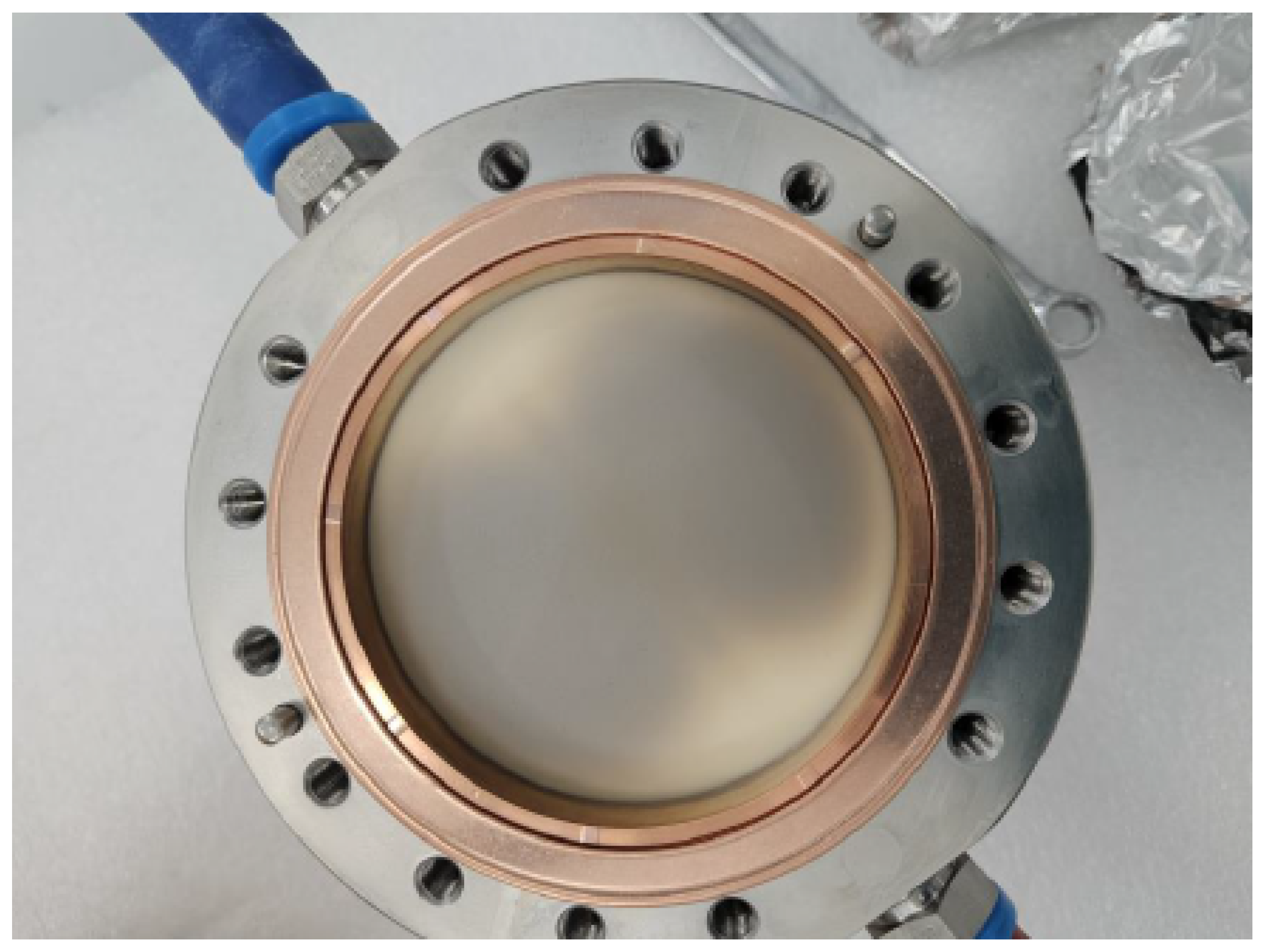
Figure 7.
Images of the first four irises of ACC2.
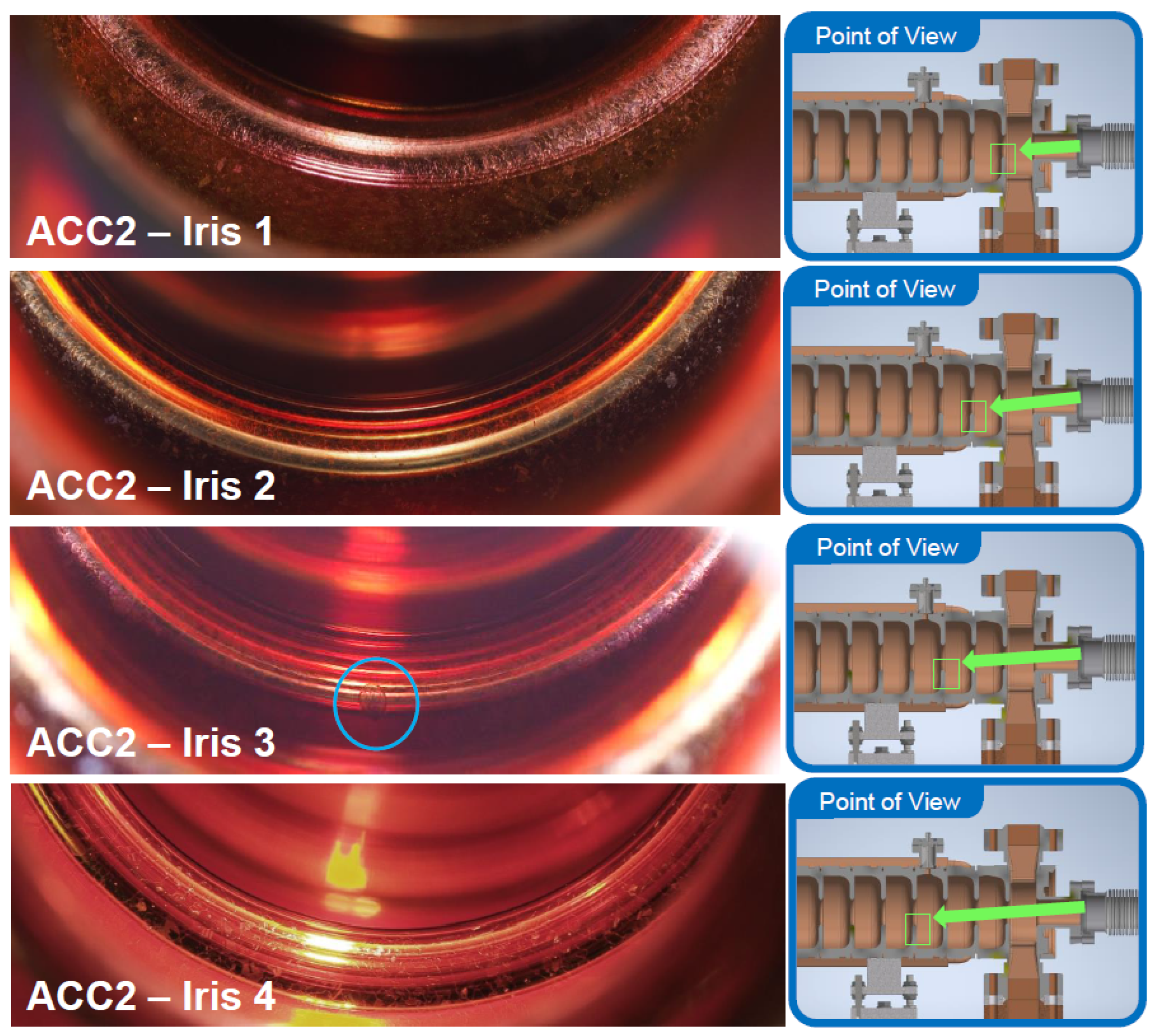
Figure 8.
Photo of the RF pickup installed in the accelerating structures.
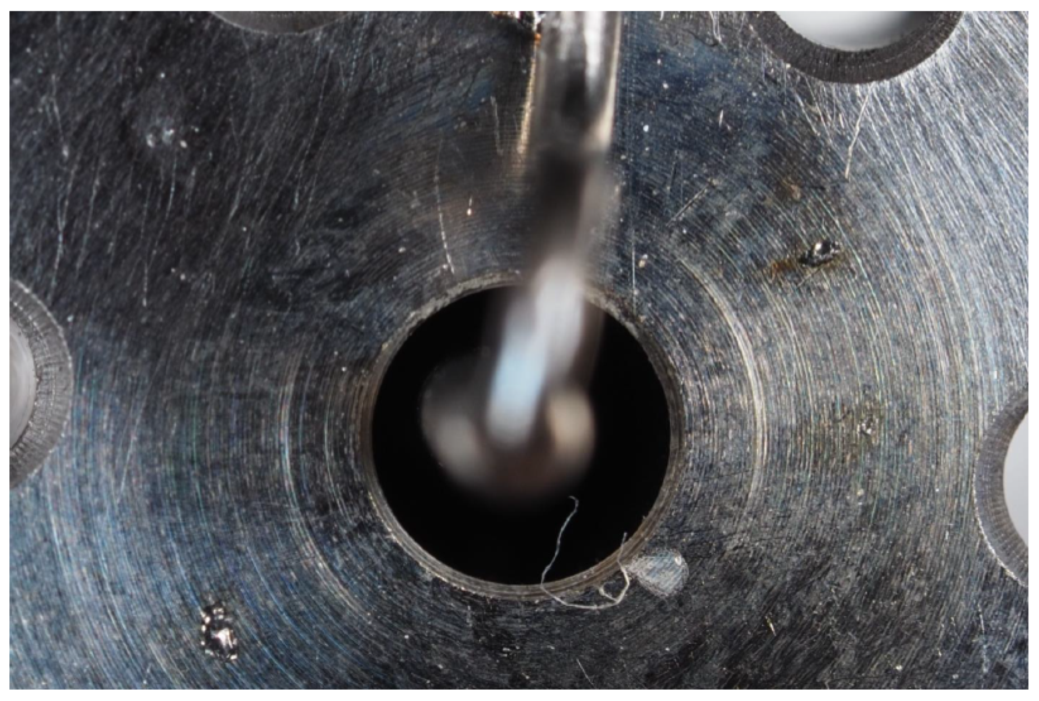
Figure 9.
Klystron power output into the RF structures (FBU, ACC1, ACC2 and ACC3, with or without SLED until April 2025.
Figure 9.
Klystron power output into the RF structures (FBU, ACC1, ACC2 and ACC3, with or without SLED until April 2025.
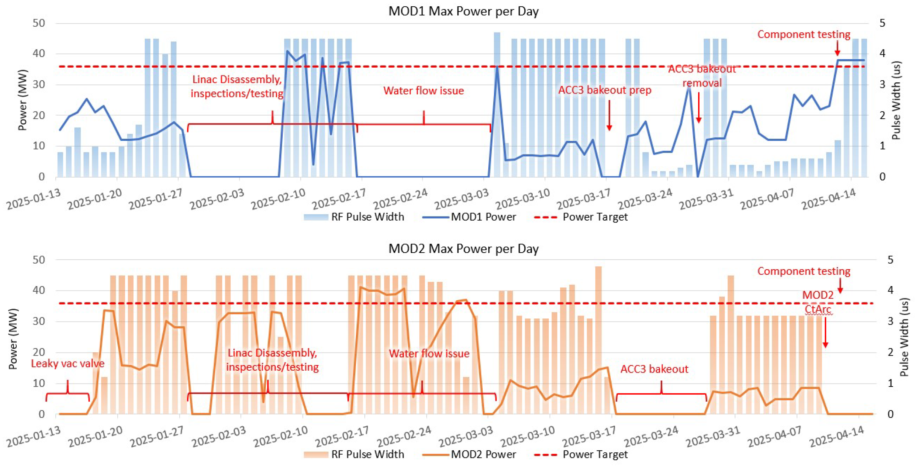
Figure 10.
RF power sustained by ACC1, ACC2 and ACC3, with or without SLED until April 2025.
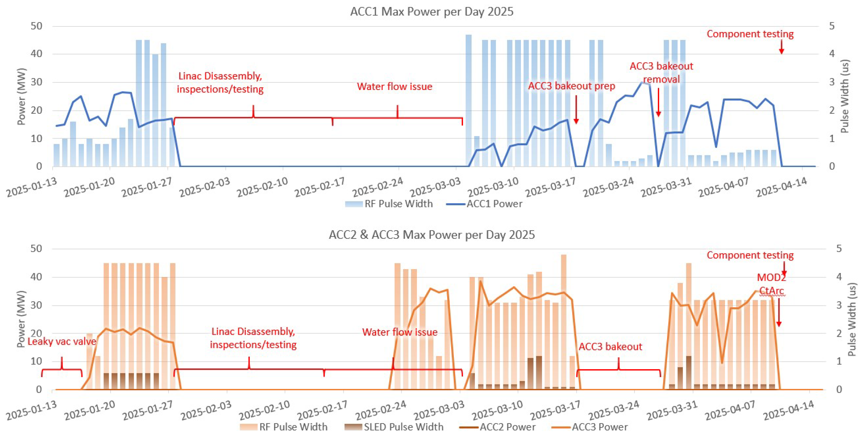
Figure 12.
ACC1, ACC2&3 power - timeline and regression in stability due to a severe breakdown forcing a full methodical RF conditioning process.
Figure 12.
ACC1, ACC2&3 power - timeline and regression in stability due to a severe breakdown forcing a full methodical RF conditioning process.
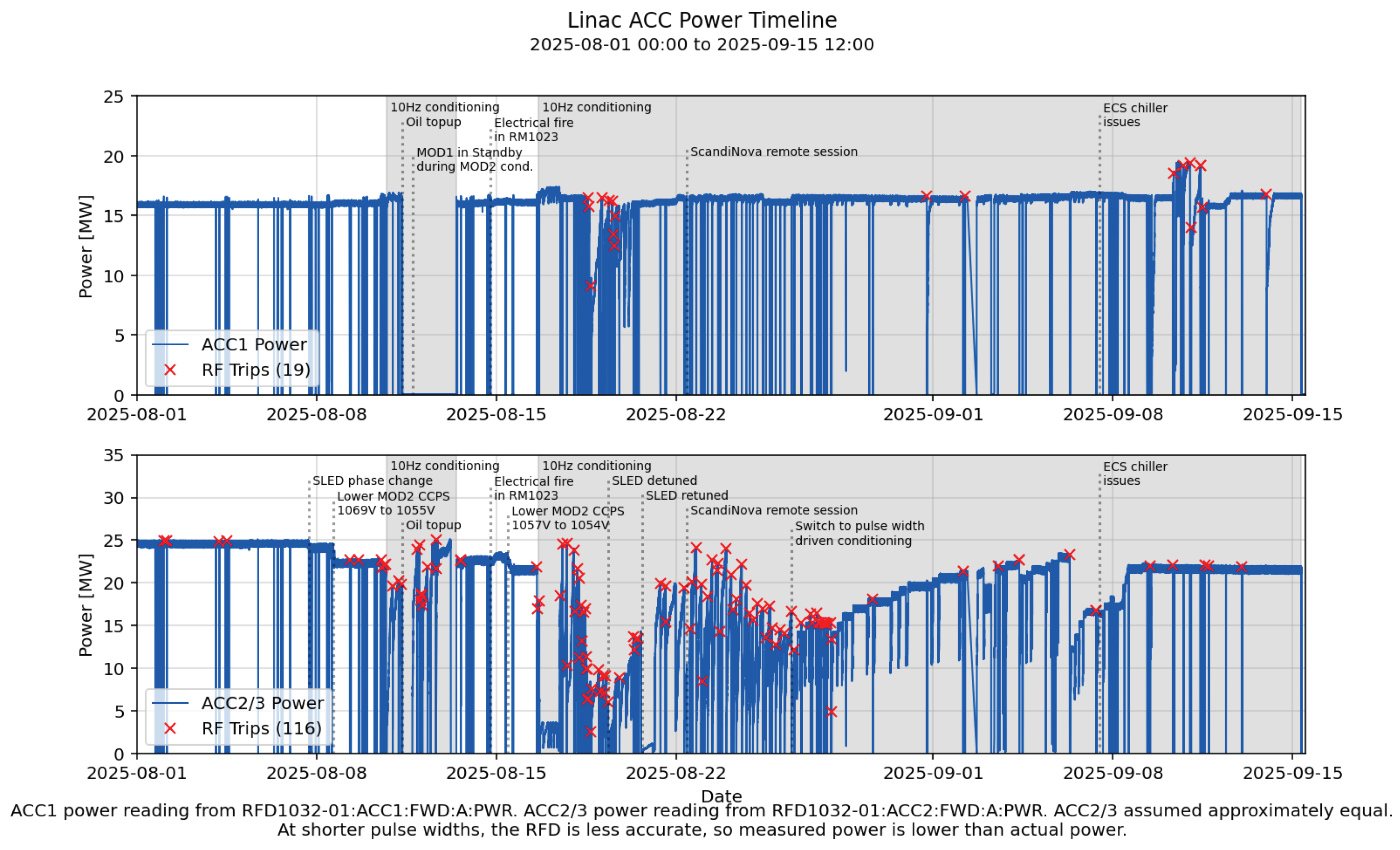
Figure 13.
RF conditioning of the spinner load for ACC1. The RF power in MW (blue) is steadily increased as long as the pressure in Torr (orange) stayed below the threshold for the specified dwell time.
Figure 13.
RF conditioning of the spinner load for ACC1. The RF power in MW (blue) is steadily increased as long as the pressure in Torr (orange) stayed below the threshold for the specified dwell time.
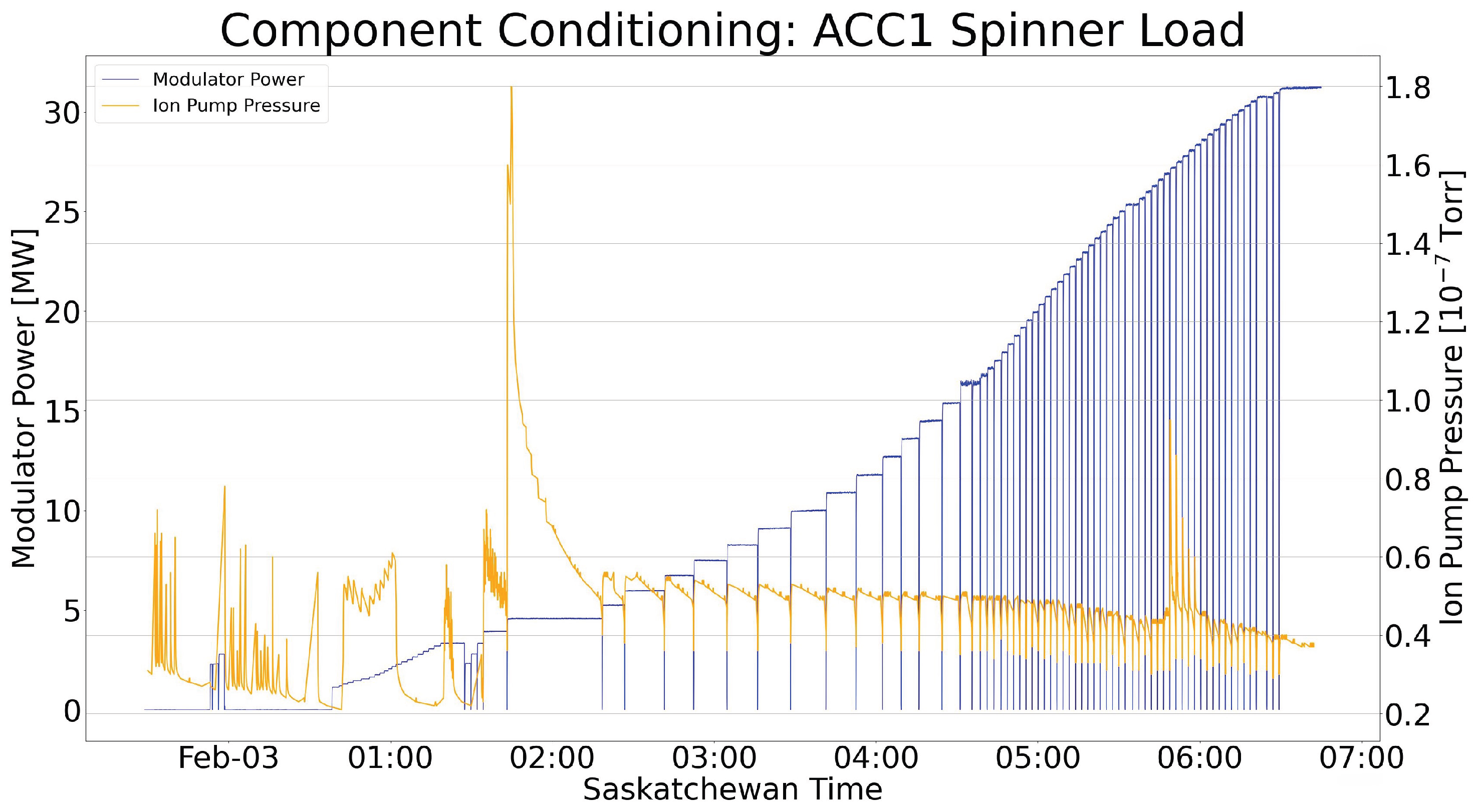
Figure 14.
Incident RF pulse (solid orange), reflected pulse (dashed green), and transmitted pulse (dotted blue) of ACC1 (without SLED) as recorded by the oscilloscope. The corresponding detected edges for each waveform are marked using the same colors.
Figure 14.
Incident RF pulse (solid orange), reflected pulse (dashed green), and transmitted pulse (dotted blue) of ACC1 (without SLED) as recorded by the oscilloscope. The corresponding detected edges for each waveform are marked using the same colors.
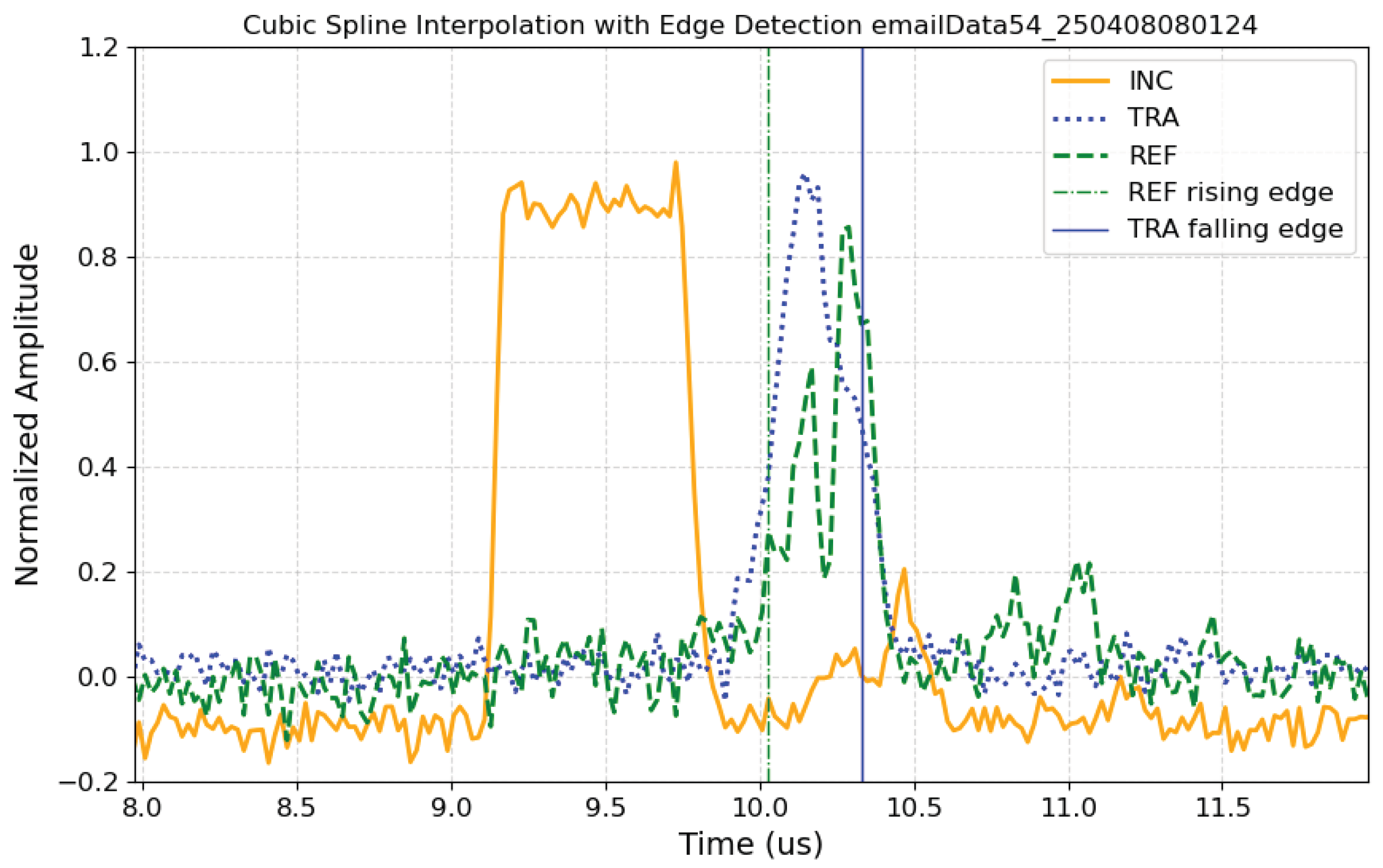
Figure 15.
Estimated location of the RF breakdown within the accelerator structure for one event, occurring at cell 75 (2.50 m from the structure entrance).
Figure 15.
Estimated location of the RF breakdown within the accelerator structure for one event, occurring at cell 75 (2.50 m from the structure entrance).
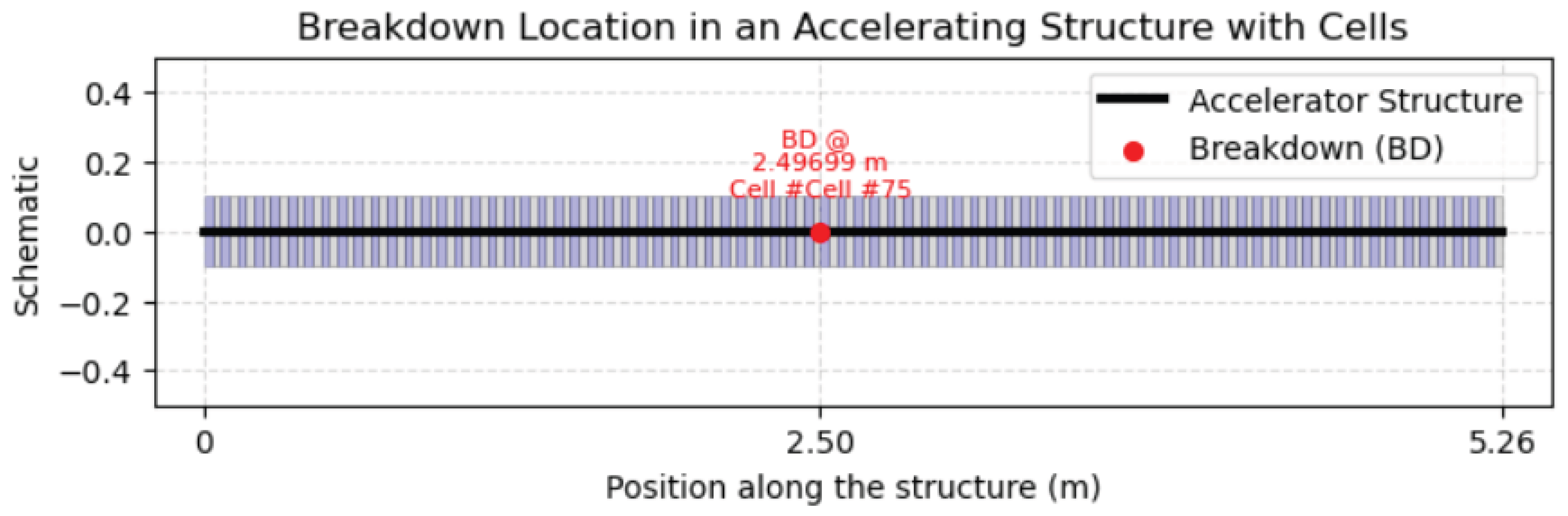
Figure 16.
RF localization hardware schematic.
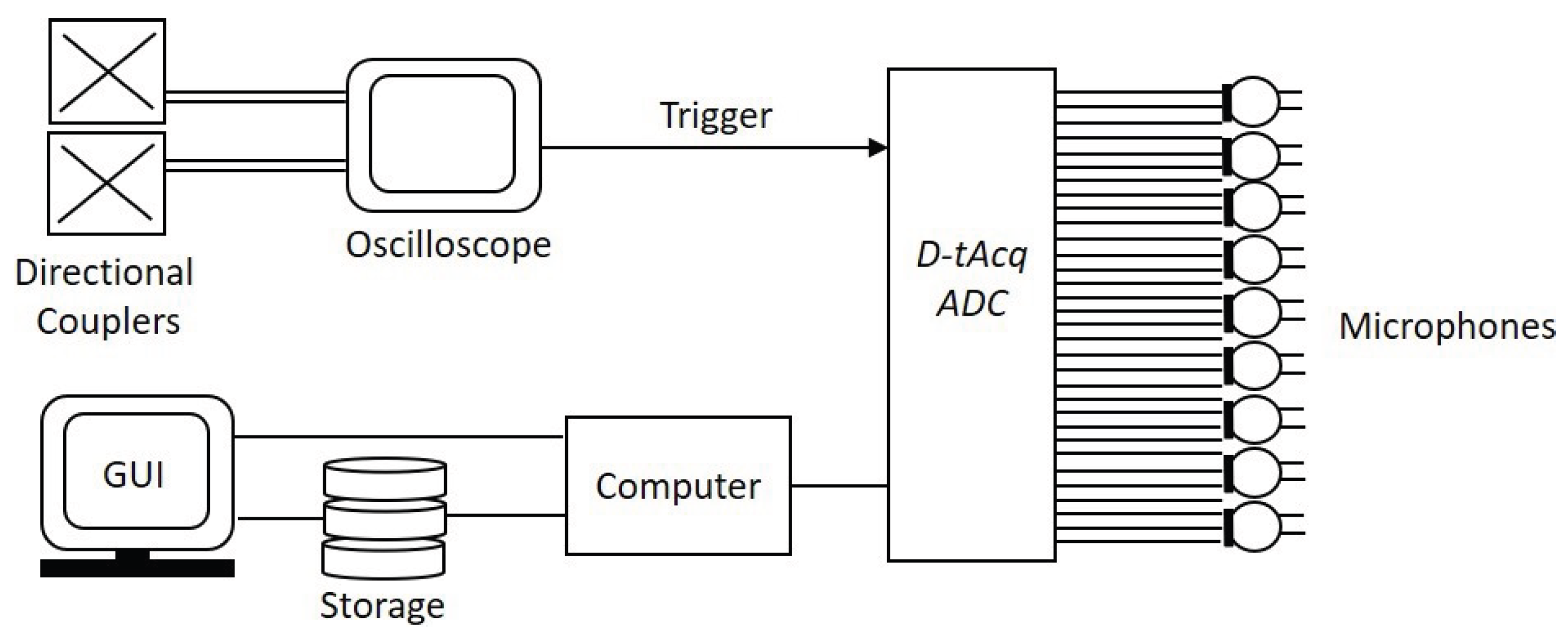
Figure 17.
An amplitude (arb. unit) plot of a set of microphone data during an RF breakdown versus the cell number of where they are mounted on the ACC3 RF structure. The probable location of the arc within ACC3 is cell 64.
Figure 17.
An amplitude (arb. unit) plot of a set of microphone data during an RF breakdown versus the cell number of where they are mounted on the ACC3 RF structure. The probable location of the arc within ACC3 is cell 64.
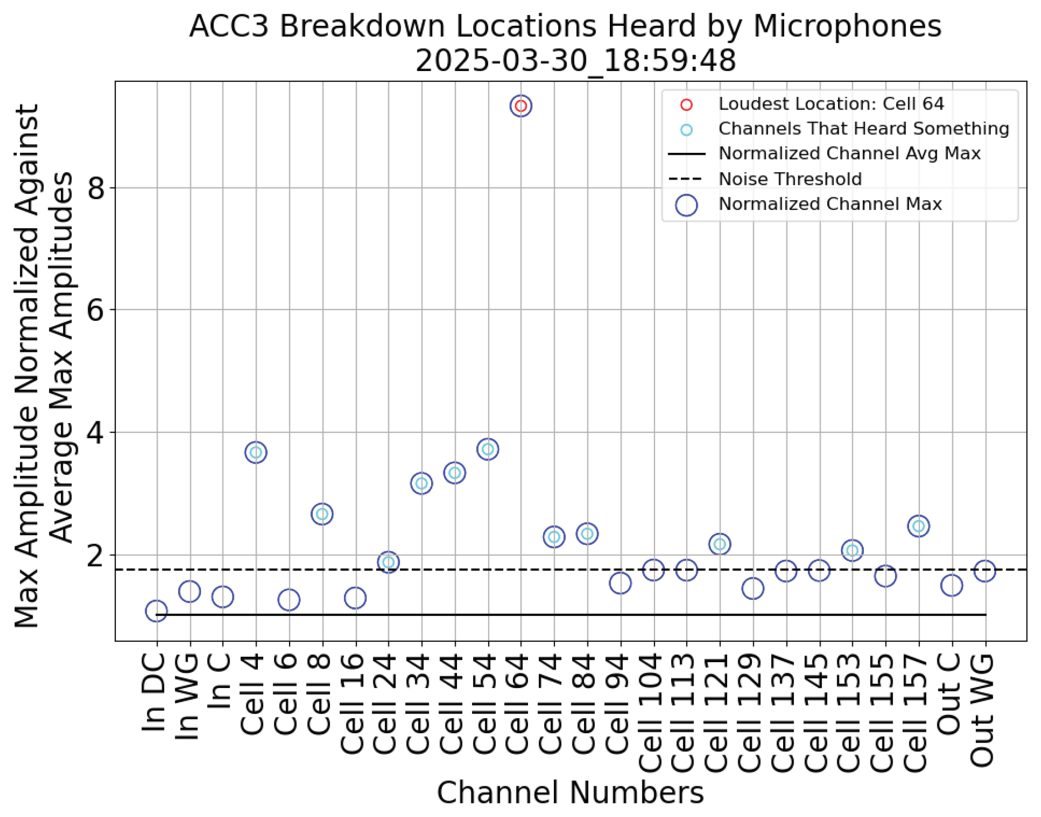
Figure 18.
A heatmap plot from a data set of microphones after an RF breakdown in Cell 64. The sound wave propagation on both sides of the identified location of the RF breakdown is picked up by the other microphones at different times.
Figure 18.
A heatmap plot from a data set of microphones after an RF breakdown in Cell 64. The sound wave propagation on both sides of the identified location of the RF breakdown is picked up by the other microphones at different times.
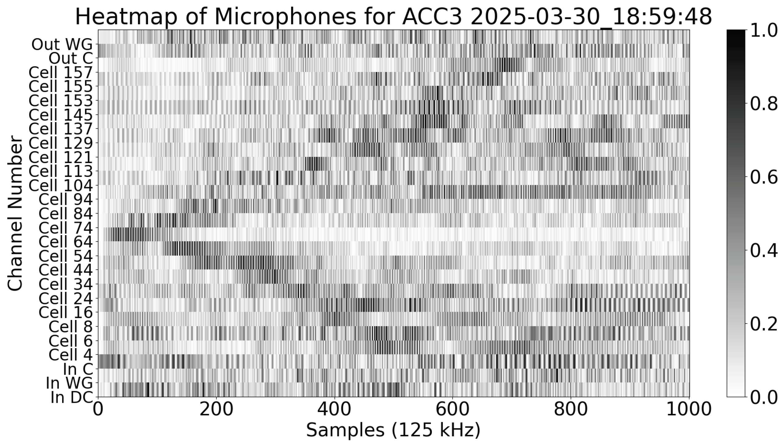
Figure 19.
Breakdown localization distribution in ACC2 for events collected between the 9th of June until 25th of August. Blue and red bars represent events reconstructed with directional coupler and microphone data respectively.
Figure 19.
Breakdown localization distribution in ACC2 for events collected between the 9th of June until 25th of August. Blue and red bars represent events reconstructed with directional coupler and microphone data respectively.
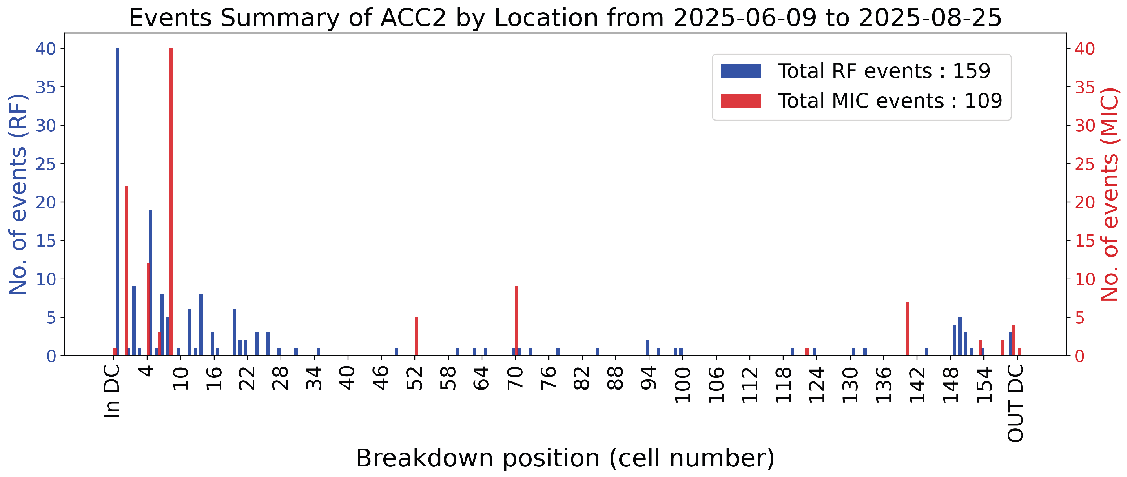
Figure 20.
Daily summary of structures showing average RF power (grey line, left axis), pulse length (blue bars, right axis), and number of breakdown events detected by the RF method (black bars) and by microphones (red bars). The plot illustrates how variations in power and pulse length correlate with the frequency of detected breakdowns, highlighting differences between the two diagnostic techniques.
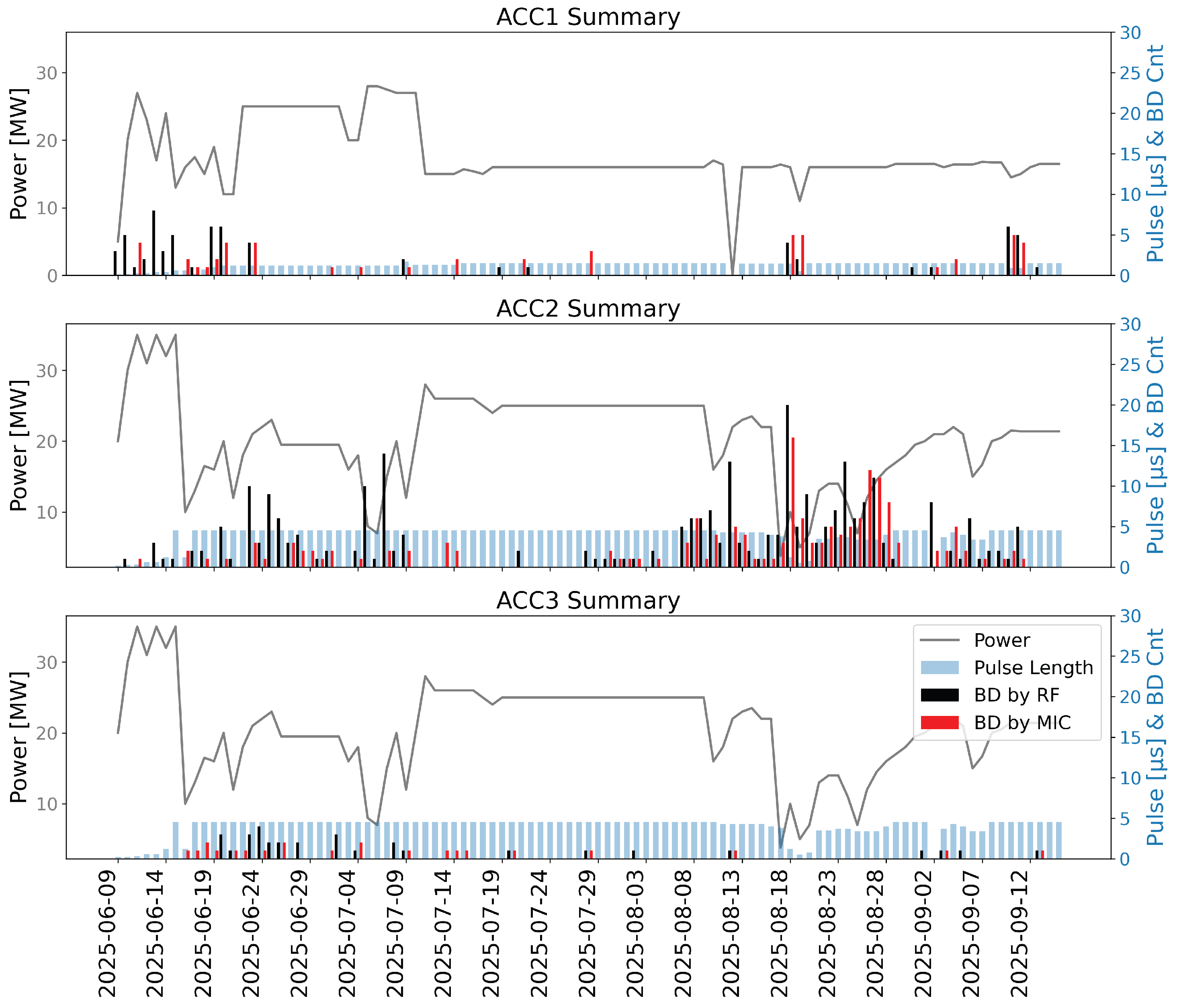
Figure 21.
Breakdown rate for structures as a function of time between June and September 2025. The bars represent the rates calculated from RF detection (blue) and microphone measurements (red). The dashed blue line indicates the exponential moving average(EMA) applied to RF data and The dashed red line indicates the EMA applied to MIC data, showing the trend in breakdown rate evolution.
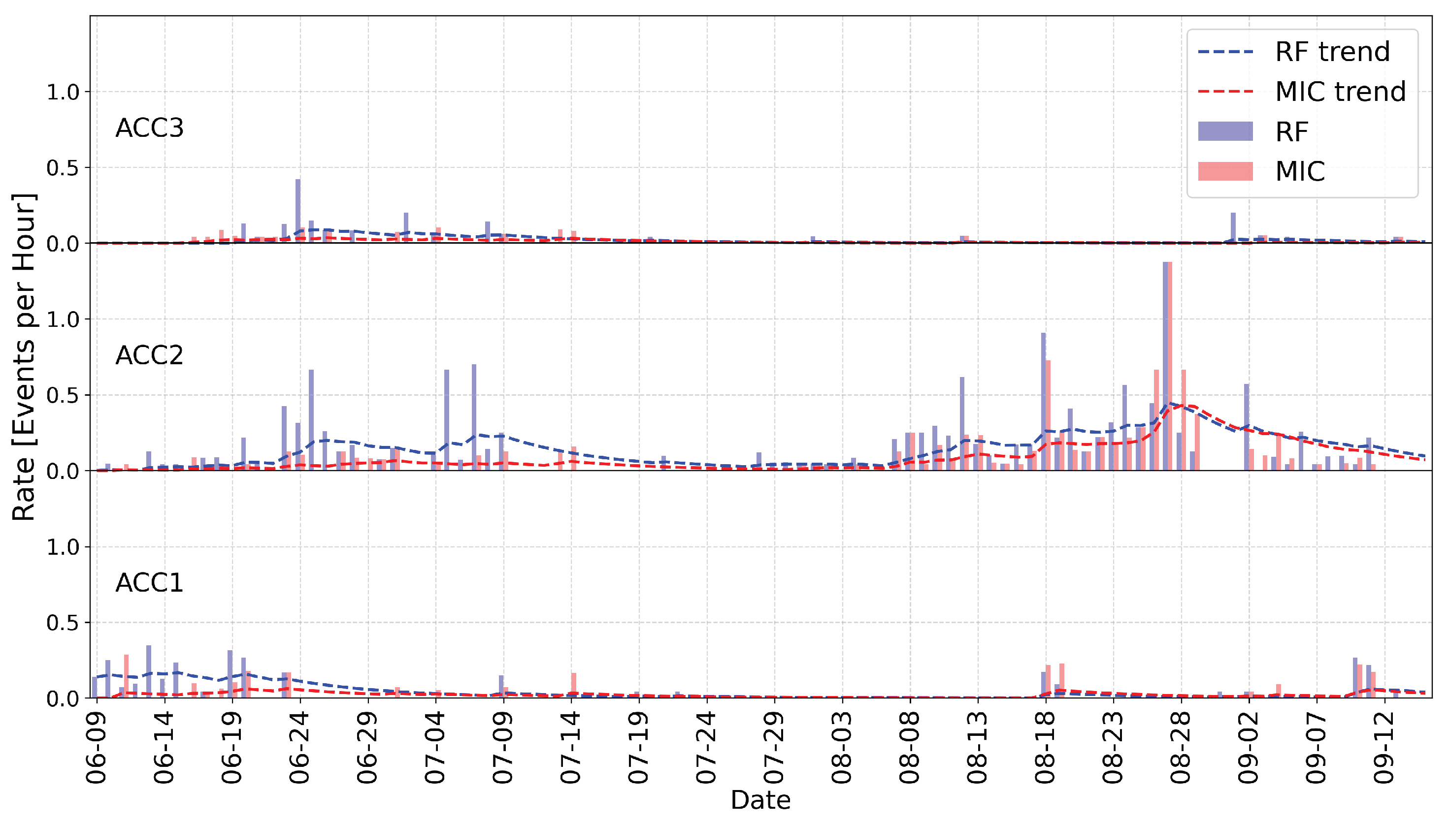
Figure 22.
YAG screen damaged by an over-focused electron beam from the electron source at 90 keV.
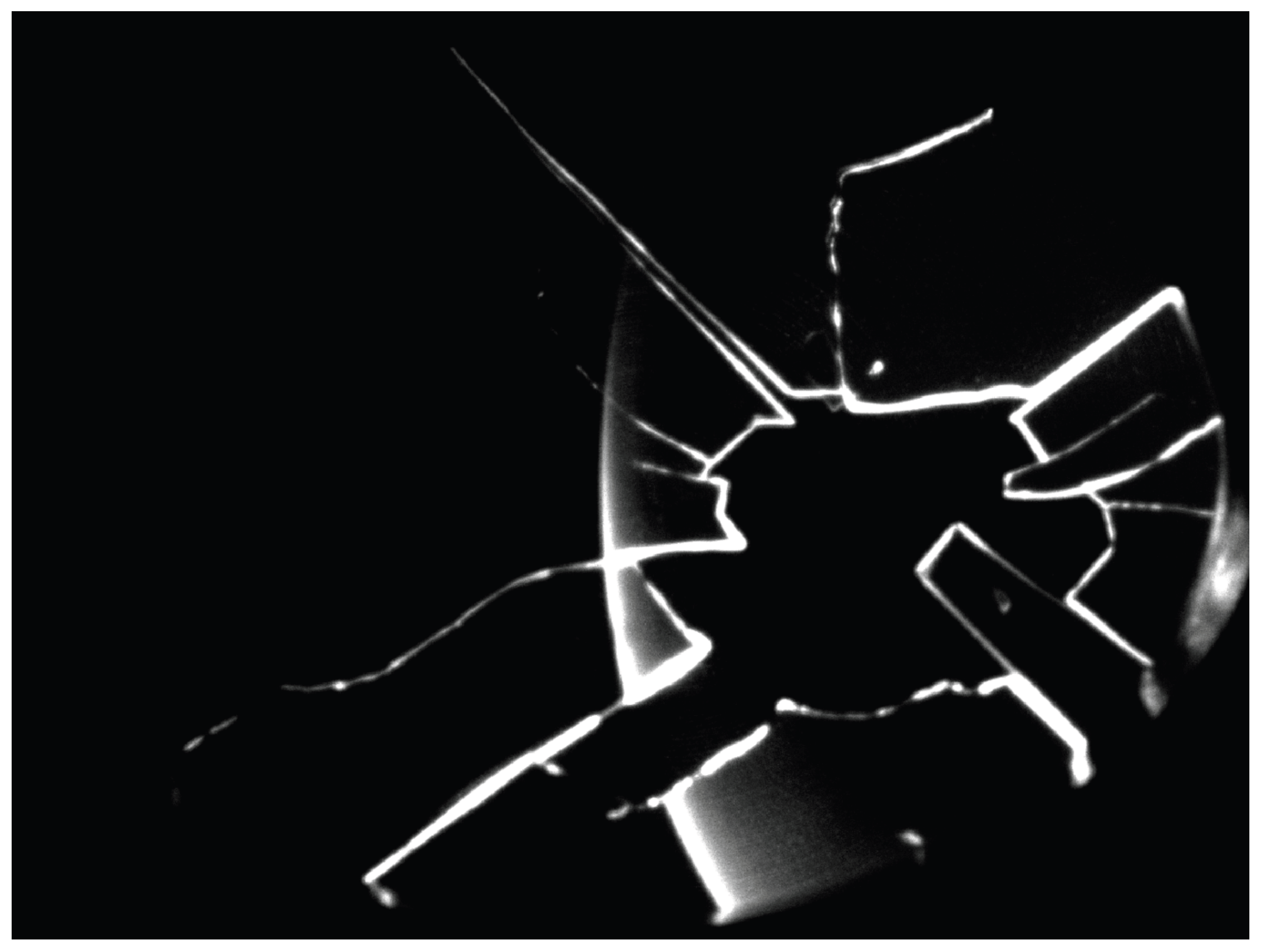
Figure 23.
Image of the electron gun cathode.
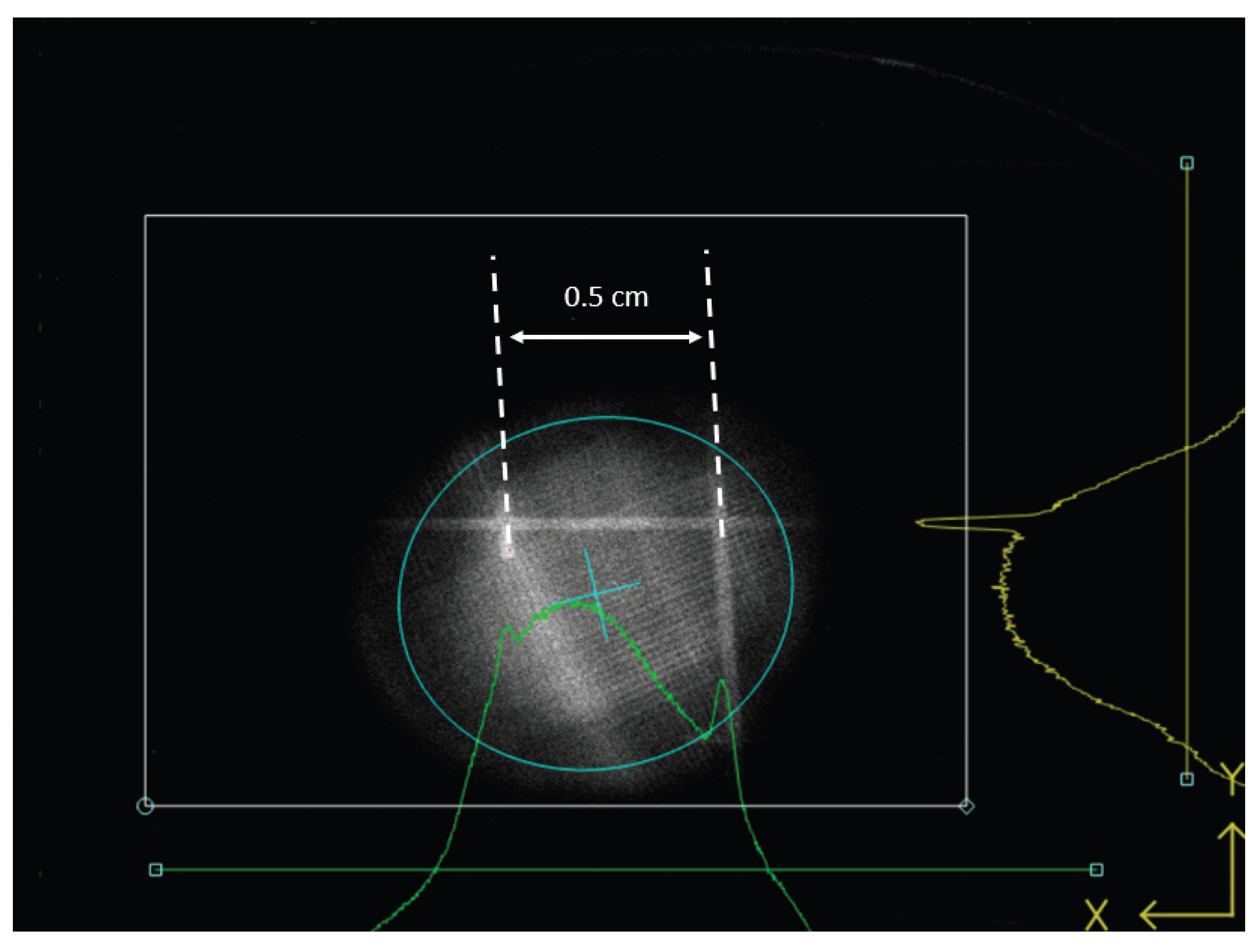
Figure 24.
LINAC beam energy spread measurement using a YAG screen and CCD camera. This measurement shows an energy spread that is acceptable to the booster. Oddly, there was a double-bump structure at the time of this measurement. The structure would vary with LINAC setup and some measurements had a more pronounced low-energy tail.
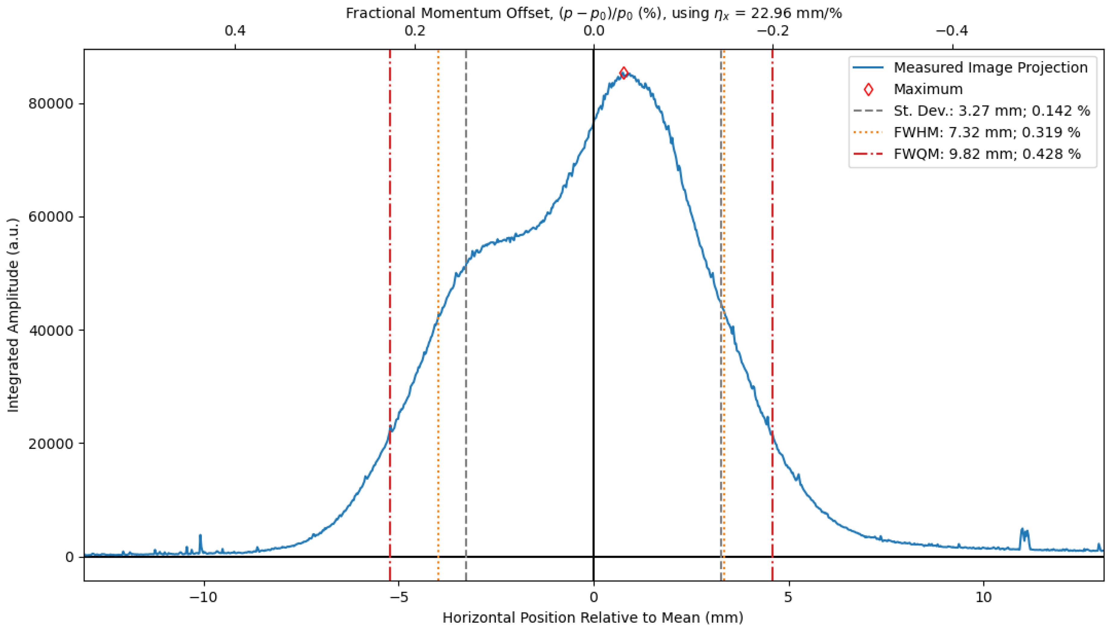
Figure 25.
Energy centroid stability measurement over about 80 minutes showing the centroid energy mostly within ±0.1%.
Figure 25.
Energy centroid stability measurement over about 80 minutes showing the centroid energy mostly within ±0.1%.

Figure 26.
The horizontal beam size, represented as the beam variance, plotted against the change in strength of a defocusing quadrupole for the old and new LINAC. Fits are done to calculate the horizontal normalized emittance.
Figure 26.
The horizontal beam size, represented as the beam variance, plotted against the change in strength of a defocusing quadrupole for the old and new LINAC. Fits are done to calculate the horizontal normalized emittance.
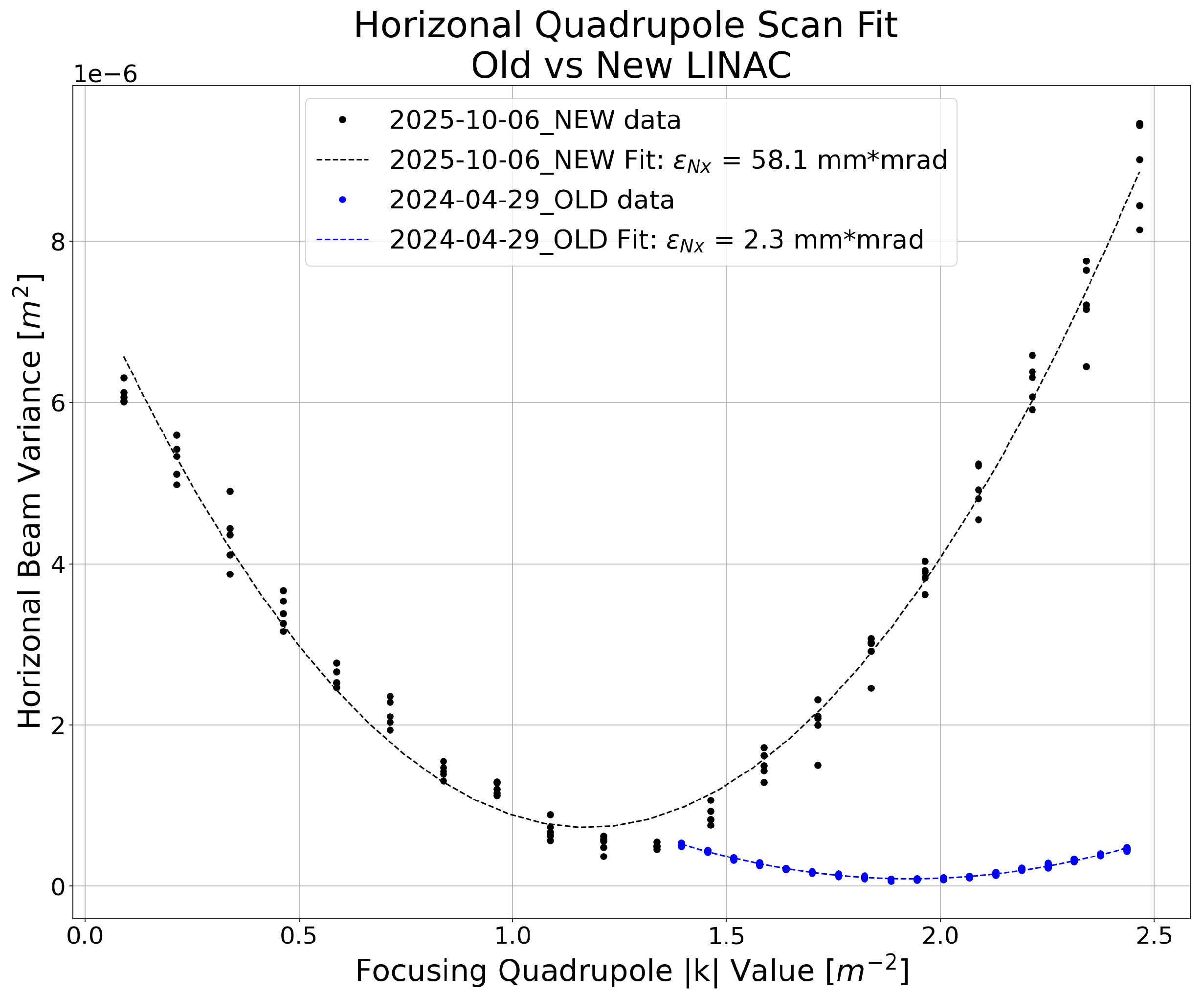
Figure 27.
The vertical beam size, represented as the beam variance, plotted against the change in strength of a focusing quadrupole for the old and new LINAC. Fits are done to calculate the vertical normalized emittance.
Figure 27.
The vertical beam size, represented as the beam variance, plotted against the change in strength of a focusing quadrupole for the old and new LINAC. Fits are done to calculate the vertical normalized emittance.
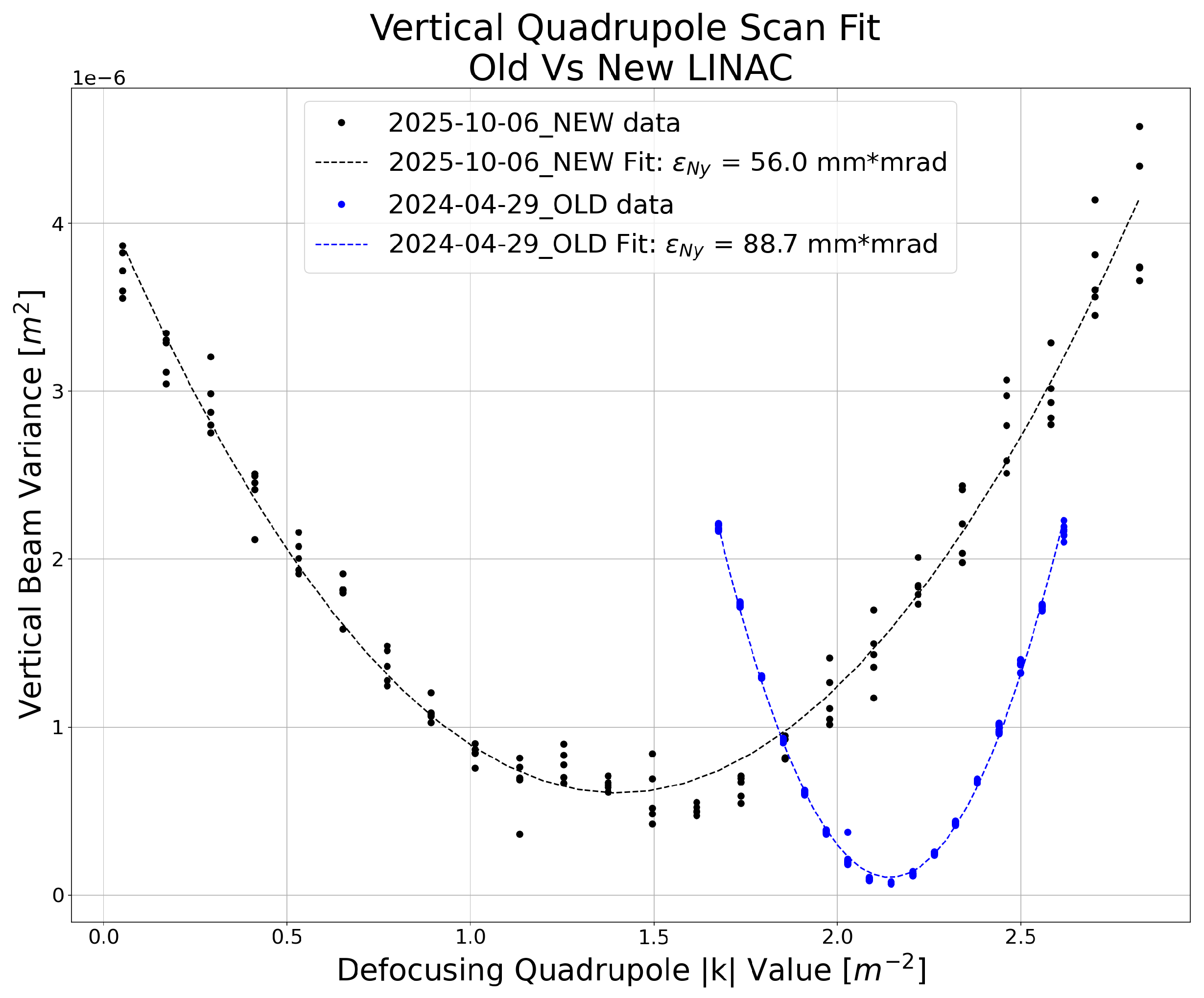
Figure 28.
LINAC frequency variation test on Aug. 9, 2025. The horizontal beam profile at the camera downstream of the ECS [orange] is show alongside the SR RF frequency [grey] and the SLED water temperature [blue] (all the structure temperatures were varies by the same step size).
Figure 28.
LINAC frequency variation test on Aug. 9, 2025. The horizontal beam profile at the camera downstream of the ECS [orange] is show alongside the SR RF frequency [grey] and the SLED water temperature [blue] (all the structure temperatures were varies by the same step size).


Table 1.
Conversion of power in the 5.5 m long ACC cavity to the equivalent of the maximum electric fields on axis and on the surface. The total gain in beam energy is provided.
Table 1.
Conversion of power in the 5.5 m long ACC cavity to the equivalent of the maximum electric fields on axis and on the surface. The total gain in beam energy is provided.
| CST | Analytic | ||
|---|---|---|---|
| E peak center | Energy gain | ||
| MW | MV/m | MV/m | MeV |
| 5 | 11.1 | 6.0 | 31.5 |
| 10 | 15.6 | 8.5 | 44.6 |
| 15 | 19.1 | 10.5 | 54.6 |
| 20 | 22.1 | 12.1 | 63.0 |
| 25 | 24.7 | 13.5 | 70.0 |
| 30 | 27.1 | 14.8 | 77.0 |
| 35 | 29.2 | 16.0 | 83.4 |
Table 2.
Conversion of power in the 50 cm long FBU structure to the equivalent of the maximum electric fields on axis and on the surface.
Table 2.
Conversion of power in the 50 cm long FBU structure to the equivalent of the maximum electric fields on axis and on the surface.
| CST | ||
|---|---|---|
| E peak center | ||
| MW | MV/m | MV/m |
| 1 | 7.5 | 5.2 |
| 2.5 | 11.9 | 8.2 |
| 4 | 15.1 | 10.4 |
| 5 | 16.9 | 11.9 |
Table 3.
Summary table with main parameters and results of the RF test and components tested.
| Test Date | Component | Starting Vacuum (Torr) |
Vacuum At Max Power (Torr) |
Duration (h) |
RF Power (MW) |
Result |
|---|---|---|---|---|---|---|
| Jan 30th to Jan 31st |
ACC2 load (CML) |
5.7 | 36 | Pass | ||
| Jan 31st | ACC2 directional coupler (Spinner) |
7 | 38 | Pass | ||
| Feb 1st | ACC1 directional coupler (Spinner) |
5.4 | 38 | Pass | ||
| Feb 1st to Feb 2nd & Feb 3rd |
ACC3 directional coupler (Spinner) |
8.6 + 3.2 | 38 | Pass* | ||
| Feb 2nd | ACC3 load (CML) |
7.3 | 38 | Pass | ||
| Feb 2nd to Feb 3rd |
ACC1 load (Spinner) |
5 | 38 | Pass | ||
| Feb 4th to Feb 5th & Feb 6th to Feb 7th |
ACC2 Load (Spinner) |
– | – | 2.5 | Fail* | |
| Feb 5th | ACC3 Load (Spinner) |
– | – | 4.8 | Fail | |
| Feb 5th to Feb 6th |
FBU Load (Spinner) |
5 | 38 | Pass | ||
| Feb 6th | ECS Load (Spinner) |
11 | 38 | Pass | ||
| Feb 18th to Feb 19th |
Spare directional coupler (Spinner) |
23 | 38 | Pass | ||
| Feb 20th to Feb 21st |
FBU Window (Spinner) |
21 | 38 | Pass | ||
| Apr 16th to Apr 18th |
ECS Window (Spinner) |
16 | 38 | Pass | ||
| Apr 23rd to Apr 24th & Apr 25th to Apr 28th |
SLED Window (Spinner) |
75 | 38 | Pass*,** | ||
| Apr 28th to Apr 29th |
ACC1 Window (Spinner) |
– | – | 4.2 | Fail |
* These components received multiple rounds of RF conditioning before passing or failing. ** Although this window passed, it was decided against re-installing it.
Table 4.
Summary table of the main parameters required in the technical specification and the results achieved.
Table 4.
Summary table of the main parameters required in the technical specification and the results achieved.
| Requirement | Technical Specification | Technical Specification |
|---|---|---|
| Reached | ||
| Electron energy | 250 MeV | 152 MeV |
| Beam production in Recovery Mode | 180 MeV in RF failure mode | No |
| Beam macrobunch repetition rate | 1 Hz | 1 Hz |
| Modulator/klystron repetition rate | 10 Hz | 10 Hz |
| RF frequency | 500.04 ± 0.005 MHz | 500.04 ± 0.005 MHz |
| 3000.24 ± 0.030 MHz | 3000.24 ± 0.030 MHz | |
| Beam charge Multibunch per 500 MHz bunch | > 0.08 nC (distributed in one or two 3 GHz bunches) | Yes |
| Multibunch train length | 1 to 70 bunches at 500 MHz with 2 ns spacing (2 to 140 ns) | 1 to 35 bunches at 500 MHz with 2 ns spacing (2 to 70 ns) |
| Center energy stability pulse to pulse | < 0.1 % rms | < 0.1 % rms |
| Energy spread | < 0.5 % rms | 0.15 % rms |
| Normalized emittance | < 50 (1 in x/y) | 52.5/55.5 (in x/y) |
| Pulse to pulse beam position variation | 0.2 mm rms | < 0.1 % rms |
| Pulse to pulse beam angle variation | 0.05 mrad rms | Not tested |
| Beam charge Single Bunch per 500 MHz bunch | > 1.5 nC (distributed in one or two 3 GHz bunches) | Not tested |
| Single Bunch bunch length | 1 ns | Not tested |
Disclaimer/Publisher’s Note: The statements, opinions and data contained in all publications are solely those of the individual author(s) and contributor(s) and not of MDPI and/or the editor(s). MDPI and/or the editor(s) disclaim responsibility for any injury to people or property resulting from any ideas, methods, instructions or products referred to in the content. |
© 2026 by the authors. Licensee MDPI, Basel, Switzerland. This article is an open access article distributed under the terms and conditions of the Creative Commons Attribution (CC BY) license (http://creativecommons.org/licenses/by/4.0/).
Copyright: This open access article is published under a Creative Commons CC BY 4.0 license, which permit the free download, distribution, and reuse, provided that the author and preprint are cited in any reuse.


