A Two-Level Relative-Entropy Theory for Isotropic Turbulence Spectra: Fokker–Planck Semigroup Irreversibility and WKB Selection of Dissipation Tails

1. Introduction

The concept of the energy cascade in three-dimensional homogeneous isotropic turbulence traces back to Kolmogorov’s seminal 1941 work (Kolmogorov, 1941). Energy is injected at large scales by external forcing, transferred hierarchically toward smaller scales through the inertial subrange, and ultimately converted into heat by viscous dissipation. To describe this process, Kolmogorov introduced a self-similarity hypothesis depending only on the mean energy dissipation rate $\epsilon$ and the kinematic viscosity $\nu$, thereby deriving the inertial-range energy spectrum $E\left(k\right)=C_K\hspace{0.17em}{\epsilon }^{2/3}\hspace{0.17em}{k}^{-5/3},$ where $k$denotes the wavenumber and $C_K$ is the Kolmogorov constant. This framework underpins Batchelor’s theory of homogeneous turbulence (Batchelor, 1953) and has served as a cornerstone for numerous subsequent statistical theories of turbulence. At the same time, Kolmogorov’s theory is essentially a scaling argument confined to the inertial subrange and is theoretically silent about the spectral shape across the full wavenumber range, including the dissipation range. To bridge this gap, spectral closure theories based on the Lin or Kármán–Howarth equations (e.g., DIA, LET) have been developed (McComb, 2017; Zhou, 2021).

As practical models for spectra including the dissipation range, Pao’s model (Pao, 1965) and Pope’s empirical spectral function (Pope, 2000) are widely used. While preserving the inertial-range $k^{-5/3}$ scaling, these models introduce an exponential cutoff from around the Kolmogorov wavenumber $k_d$ toward higher wavenumbers, reproducing DNS data with high fidelity (Verma et al., 2017; Dos Santos et al., 2022). Recent analyses of high-Reynolds-number DNS and experimental data further indicate that the dissipation-range spectrum is not well described by a simple $\mathrm{e}\mathrm{x}\mathrm{p}(-\beta k)$form, but rather by a stretched exponential,

$E\left(k\right)\sim C_K\hspace{0.17em}{\epsilon }^{2/3}\hspace{0.17em}{k}^{-5/3}\mathrm{e}\mathrm{x}\mathrm{p}\left[-\beta {\left({\displaystyle \frac{k}{k_d}}\right)}^m\right],$as reported in, e.g., Gorbunova et al. (2020), Buaria et al. (2020), and Verma et al. (2017). Here the exponent $m$typically lies in the range $m\in [4/\mathrm{3,3}/2]$ and is suggested to vary with flow conditions and Reynolds number. This “non-universality of $m$” confronts turbulence theory—historically oriented toward universal scaling—with fundamental questions: why does the dissipation-range spectrum assume a stretched-exponential, rather than a simple $\mathrm{e}\mathrm{x}\mathrm{p}(-\beta k)$, form; why is $m$constrained to the relatively narrow interval $4/3\le m\le 3/2$; what is the “selection principle” that determines $m$; and to what extent can $m$be uniquely fixed from Navier–Stokes dynamics? Existing spectral models, in many cases, rely on empirical fitting or semi-empirical scaling assumptions, and thus remain insufficient as first-principles derivations (Solsvik & Jakobsen, 2017).

In parallel, a rapidly growing line of research has begun to reinterpret turbulence not merely as an “energy cascade,” but as a process of information generation and transfer. For instance, a “hydrodynamic entropy” defined for Euler turbulence has been shown to quantify the formation and dissolution of coherent structures (Verma & Chatterjee, 2022), and within information thermodynamics, universal lower bounds have been established for inter-scale information flow in shell-model turbulence (Tanogami & Araki, 2024). Moreover, for multi-field turbulence, studies inspired by quantum information theory have introduced von Neumann entropy and entanglement entropy to simultaneously characterize the strength of nonlinear mode coupling and the direction of energy transfer (Yatomi & Nakata, 2025). Collectively, these developments foreground a shared perspective: in turbulence, energy dissipation is intrinsically tied to information generation and loss, in a manner complementary to Kolmogorov theory and classical spectral closures.

However, most information-theoretic approaches have focused less on directly determining the specific functional form of the energy spectrum than on quantifying information flows associated with the cascade or elucidating the information-geometric structure of nonequilibrium fluctuations. Consequently, an “entropy principle for determining the energy spectrum”—namely, a program that (i) defines an appropriate turbulence entropy $S_{\mathrm{t}\mathrm{u}\mathrm{r}\mathrm{b}}$, (ii) proves that its evolution satisfies $d{S}_{\mathrm{t}\mathrm{u}\mathrm{r}\mathrm{b}}/dt\ge 0$ (an $H$-theorem), and (iii) derives the realized energy spectrum $E\left(k\right)$ from a corresponding entropy variational principle—has not yet been established in a fully satisfactory form.

To bridge the remaining gap between “dynamics (admissibility)” and “information-theoretic selection (realizability)” in turbulence spectral theory, we propose a two-level theory that integrates a Lin-equation-based coarse-graining with a relative-entropy principle in logarithmic wavenumber space. The central idea is as follows: (i) within the class of autonomous conservative Fokker–Planck (FP) semigroups consistent with Navier–Stokes dynamics, we establish an irreversible structure via an $H$-theorem; (ii) in the dissipation range, we analyze an effective stationary problem incorporating killing (absorption) by WKB methods to strongly constrain the admissible tail classes; and (iii) within the resulting admissible class, we identify the exponent that minimizes additional information by formulating it as a relative-entropy minimization problem.

In the first stage (the dynamical level), we start from the fact that the energy spectrum $E(k,t)$ of three-dimensional homogeneous isotropic turbulence satisfies the Lin equation. Based on the mapping $\xi =\mathrm{l}\mathrm{n}\left(k/k_0\right)$ and a locality (near-neighbor) assumption for the flux, we introduce in a consistent manner the scale-space probability density $P(\xi ,t)$ and the probability current $J(\xi ,t)$. By making explicit the boundary conditions and the regularity of coefficients—most notably, a positive lower bound for the diffusion coefficient—we construct a framework in which integration by parts and relative-entropy estimates are mathematically justified. As a result, under an autonomous conservative FP semigroup, the relative turbulence entropy becomes a Lyapunov functional and monotonicity (an $H$-theorem) holds rigorously.

In the second stage (the selection level), we aim to determine the dissipation-range spectral shape in a verifiable manner while avoiding the intrinsic difficulty of directly treating the “nonzero-flux NESS itself” as a limit of a conservative semigroup. To this end, we introduce, in the dissipation range, an effective stationary equation that includes killing (absorption), and evaluate its high-wavenumber tail via WKB (eikonal) analysis. This yields a strong constraint: the dissipation tail must reduce to a stretched-exponential form. Nonetheless, the exponent (or an equivalent parameter) still remains as a candidate set.

We therefore define a physically meaningful “global domain” for comparing candidate families by introducing the lower endpoint ${\xi }_{-}=\mathrm{l}\mathrm{n}{k}_f$, where $k_f$ is a representative forcing-band wavenumber, and setting

$\xi \in [{\xi }_{-},\mathrm{\infty }).$

We then unify the integration domain of the KL functional to this common lower bound, thereby avoiding any unnatural extension of the dissipation-tail shape into the low-wavenumber energy-containing range. This unification ensures that the KL distance between the reference distribution and each candidate distribution is well-defined over the entire domain and closes a mathematical loophole that would otherwise arise from mismatched lower limits.

Next, we incorporate the $m$–$\gamma$ coupling obtained as a WKB consequence in Section 4 (equivalently, $m=1+\gamma /2$) as a constraint, thereby eliminating arbitrariness associated with independent optimization over $\gamma$. Specifically, rather than adopting a two-variable optimization in $\left(m,\gamma \right)$, we reduce the identification problem to a one-dimensional optimization in $\gamma$ alone (Hyper-MaxEnt) by enforcing the coupling relation.

With these ingredients, we construct the reference distribution globally on $[{\xi }_{-},\mathrm{\infty })$ and identify ${\gamma }^{*}$ by minimizing the KL distance to the candidate family via a one-dimensional optimization; the final exponent $m^{*}$ is then determined through the coupling relation. Consequently, the exponent $m^{*}$ in this paper is not a post hoc fit parameter chosen to match observations; rather, it is defined by a verifiable logical chain consisting of (i) the irreversible structure at the dynamical level, (ii) the strong WKB constraint on the candidate set, (iii) reduction of degrees of freedom, and (iv) relative-entropy minimization.

Within this framework, our contributions can be summarized in three points. First, by coarse-graining based on the Lin equation, we establish the setting of an autonomous conservative FP semigroup and position—explicitly specifying boundary conditions and coefficient regularity—the result that the relative turbulence entropy functions as a Lyapunov functional (an $H$-theorem). Second, by extracting the dissipation range as an effective stationary problem with killing and analyzing it via WKB methods, we show that the tail must reduce to a stretched-exponential form, thereby strongly constraining the “dynamically admissible asymptotic class.” Third, after unifying the integration domain to $\left.\xi \in [{\xi }_{-},\mathrm{\infty }\right)$, we incorporate the WKB-derived $m$–$\gamma$ coupling as a constraint and formulate KL minimization as a one-dimensional optimization, providing a reduced Hyper-MaxEnt framework that identifies $m^{*}$ without externally fixing it.

The remainder of this paper is organized as follows. In Section 2, we formulate the mapping from the Lin equation to logarithmic wavenumber space and develop the conservative FP coarse-graining. In Section 3, we establish monotonicity (an $H$-theorem) for the relative turbulence entropy under an autonomous conservative FP semigroup, thereby providing the irreversible structure at the dynamical level. In Section 4, we formulate the dissipation range as an effective stationary problem with killing and derive, via WKB analysis, the stretched-exponential constraint on the dissipation tail. In Section 5, we unify the comparison domain to $[{\xi }_{-},\mathrm{\infty })$, incorporate the WKB coupling constraint, and present the final principle that identifies $m^{*}$through a one-dimensional optimization, clarifying the connection between the dynamical and selection levels.

2. Dynamical Modelling of the Turbulent Cascade

This Section formulates the first stage (dynamical level) of the proposed two-level theory. We begin with the energy-spectrum balance equation derived from the Navier–Stokes equations, namely the Lin equation. The associated energy flux in the Lin equation is intrinsically nonlocal, being defined through an integral over all wavenumbers of triadic interactions, and therefore admits no closed form in general. In this work, we regard the turbulent cascade as an aggregate of many local transfer events and coarse-grain it as an effective Markov process in logarithmic wavenumber space. In the continuous limit, this yields a Fokker–Planck (FP) equation, which provides a unified foundation for the probability current, entropy, and WKB analyses developed in subsequent Sections. A key point is that the drift and diffusion coefficients $A(\xi ,t)$ and $D(\xi ,t)$ introduced here are effective coefficients, defined as low-order moments of a coarse-grained transition kernel, rather than “exact quantities” that fully encode triadic interactions. All subsequent analysis is constructed self-consistently within this effective-theory framework.

2.1. Lin Equation and the Energy-Spectrum Budget

Let $E(k,t)$ denote the energy spectrum of three-dimensional homogeneous isotropic turbulence, and define the total kinetic energy per unit mass by

$E_{\mathrm{t}\mathrm{o}\mathrm{t}}\left(t\right)={\int }_0^{\mathrm{\infty }}E(k,t)\hspace{0.17em}dk.$

Let $T_f(k,t)$ be the spectral density of energy injection by external forcing, and let $\nu$be the kinematic viscosity. Then $E(k,t)$ satisfies the Lin equation,

${\displaystyle \frac{\partial E(k,t)}{\partial t}}+{\displaystyle \frac{\partial \mathsf{\Pi }(k,t)}{\partial k}}=T_f(k,t)-2\nu k^{2}E(k,t)$ (1)

Here $\mathsf{\Pi }(k,t)$ is the energy flux in wavenumber space; since it arises from triadic interactions, it is in general defined by a nonlocal integral.

In a statistically stationary state, ${\partial }_{t}E=0$, and (1) reduces to

${\displaystyle \frac{\partial \mathsf{\Pi }\left(k\right)}{\partial k}}=T_f\left(k\right)-2\nu k^{2}E\left(k\right)$ (2)

Define the dissipation rate $\epsilon$ by

$\epsilon =2\nu {\int }_0^{\mathrm{\infty }}{k}^{2}E\left(k\right)\hspace{0.17em}dk$ (3)

If the forcing is localized in a finite wavenumber band, and in the inertial subrange

$k_f\ll k\ll k_d$ one has $T_f\simeq 0$ while viscous dissipation is negligible, then (2) yields

$\mathsf{\Pi }\left(k\right)\simeq \epsilon (k_f\ll k\ll k_d)$ (4)

Consistently, Kolmogorov’s $-5/3$law holds:

$E\left(k\right)\simeq C_K\hspace{0.17em}{\epsilon }^{2/3}{k}^{-5/3}$ (5)

To connect with the dissipation range, define the Kolmogorov wavenumber by

$k_d={\left({\displaystyle \frac{\epsilon }{{\nu }^3}}\right)}^{1/4}$ (6)

and introduce the dimensionless wavenumber $x=k/k_d$.

2.2. Unified Spectral Representation Including the Dissipation Range

To represent the full spectrum, including the dissipation range, in a unified form, we adopt the following cutoff representation:

$E\left(k\right)=C_K\hspace{0.17em}{\epsilon }^{2/3}{k}^{-5/3}f\hspace{0.17em}\left({\displaystyle \frac{k}{k_d}}\right)$ (7)

Here $f\left(x\right)$ is a smooth function satisfying $f\left(x\right)\to 1$ for $x\ll 1$ and decaying exponentially for $x\gg 1$. In the latter part of this paper (Section 4 and Section 5), we will constrain the dynamically admissible class of $f$ via asymptotic analysis and select the remaining freedom by an information-theoretic principle.

2.3. Log-Wavenumber Space and the Definition of Probability Densities

To treat the distribution in wavenumber space on a logarithmic scale, fix a reference wavenumber $k_0>0$ and introduce

$\xi =\ln \hspace{0.17em}\left({\displaystyle \frac{k}{k_0}}\right)$ (8)

The mapping $k=k_0{e}^{\xi }$ is a $C^{\mathrm{\infty }}$-diffeomorphism between $\mathbb{R}$ and $\left(0,\mathrm{\infty }\right)$, with Jacobian

${\displaystyle \frac{dk}{d\xi }}=k\left(k=k_0{e}^{\xi }\right)$ (9)

i.e., $dk=k\hspace{0.17em}d\xi$.

Henceforth, for each time $t$, we assume that the spectrum $E(k,t)$ is measurable on $\left(0,\mathrm{\infty }\right)$ and satisfies

$E\left(k,t\right)\ge 0 (\mathrm{a}.\mathrm{e}. \mathrm{on} (0,\mathrm{\infty }))$ (10)

Define the total kinetic energy per unit mass by

$E_{\mathrm{t}\mathrm{o}\mathrm{t}}\left(t\right)={\int }_0^{\mathrm{\infty }}E\left(k,t\right)\hspace{0.17em}dk$ (11)

and assume

$0<E_{\mathrm{t}\mathrm{o}\mathrm{t}}\left(t\right)<\mathrm{\infty }$ (12)

so that normalization is well-defined.

Under the change of variables $k=k_0{e}^{\xi }$and using (9), (11) can be rewritten as

$E_{\mathrm{t}\mathrm{o}\mathrm{t}}\left(t\right)={\int }_0^{\mathrm{\infty }}E\left(k,t\right)\hspace{0.17em}dk={\int }_{-\mathrm{\infty }}^{\mathrm{\infty }}k\hspace{0.17em}E\left(k,t\right)\hspace{0.17em}d\xi$ (13)

Define the unnormalized scale density in log-wavenumber space by

$\left(\xi ,t\right)\equiv k\hspace{0.17em}E\left(k,t\right),\left(k=k_0{e}^{\xi }\right)$ (14)

By (10), $\bar{P}(\xi ,t)\ge 0$ (a.e.), and by (12) ans (13) one has $\bar{P}(\cdot ,t)\in L^1\left(\mathbb{R}\right)$ with

${\int }_{-\mathrm{\infty }}^{\mathrm{\infty }}\mathcal{P}\left(\xi ,t\right)\hspace{0.17em}d\xi =E_{\mathrm{t}\mathrm{o}\mathrm{t}}\left(t\right)$ (15)

We then define the normalized probability density in log-wavenumber space by

$P\left(\xi ,t\right)\equiv {\displaystyle \frac{\mathcal{P}\left(\xi ,t\right)}{E_{\mathrm{t}\mathrm{o}\mathrm{t}}\left(t\right)}}={\displaystyle \frac{k\hspace{0.17em}E\left(k,t\right)}{E_{\mathrm{t}\mathrm{o}\mathrm{t}}\left(t\right)}},\left(k=k_0{e}^{\xi }\right)$ (16)

By assumption (12), the right-hand side is well-defined, and (15) immediately yields the normalization

${\int }_{-\mathrm{\infty }}^{\mathrm{\infty }}P(\xi ,t)\hspace{0.17em}d\xi =1.$Conversely, from (16), for any $k>0$,

$E\left(k,t\right)={\displaystyle \frac{E_{\mathrm{t}\mathrm{o}\mathrm{t}}\left(t\right)}{k}}\hspace{0.17em}P\left(\xi ,t\right),\xi =\ln \hspace{0.17em}\left({\displaystyle \frac{k}{k_0}}\right)$ (17)

From Section 2 through Section 3, $P(\xi ,t)$ denotes the normalized probability density defined in (16), while the unnormalized quantity is always denoted by $\bar{P}(\xi ,t)$. When, from Section 4 onward, the unnormalized density becomes the primary unknown, we continue to use the same symbols $P$ and $\bar{P}$ accordingly, without redefining $P$.

2.4. Coarse-Graining: From a Jump Process to the Fokker–Planck Equation

The energy flux $\mathsf{\Pi }(k,t)$ appearing in the Lin equation originates from triadic interactions and is, in general, defined as a nonlocal integral over the entire wavenumber range. In this section, rather than retaining the full nonlocal detail, we coarse-grain the cascade as an effective transition process on the logarithmic wavenumber $\xi$, and derive, in its diffusion limit, a Fokker–Planck (FP) equation. Using a Chapman–Kolmogorov-type master equation as the starting point is not in conflict with the section title “Fokker–Planck equation”: the master equation is the fundamental evolution law for a jump process, and in the continuous limit where near-neighbor jumps (small $\mathsf{\Delta }\xi$) dominate, its generator converges to a second-order differential operator, yielding the FP equation.

2.4.1. Assumptions for the Jump Process and the Master Equation

We approximate energy transfer on the logarithmic wavenumber axis as an accumulation of “jumps from $\xi$ to $\xi +\mathsf{\Delta }\xi$,” and represent the transition by a conditional transition kernel (jump kernel)

$W(\mathsf{\Delta }\xi ;\xi ,t)\ge 0$ (18)

As explicit premises of the coarse-graining, we impose the following.

First, quasi-locality (locality): for fixed $\left(\xi ,t\right)$, the dominant transitions are concentrated in $\mid \mathsf{\Delta }\xi \mid \ll 1$, and large jumps are sufficiently suppressed. Introducing a small parameter $\delta \downarrow 0$, this may be expressed, for instance, as

${\int }_{\mid \mathsf{\Delta }\xi \mid >\eta }W(\mathsf{\Delta }\xi ;\xi ,t)\hspace{0.17em}d\left(\mathsf{\Delta }\xi \right)\underset{\delta \to 0}{\to }0 (\forall \hspace{0.17em}\eta >0)$ (19)

which signifies the vanishing of the large-jump tail probability.

Second, effective Markov property (short memory): on the coarse-grained time scale, short memory holds, and the time evolution of $\xi$ follows a Chapman–Kolmogorov-type master equation. For the normalized probability density $P(\xi ,t)$ defined in Section 2.3, the master equation takes the form

${\partial }_{t}P(\xi ,t)={\int }_{-\mathrm{\infty }}^{\mathrm{\infty }}\left[W\right(\mathsf{\Delta }\xi ;\xi -\mathsf{\Delta }\xi ,t)\hspace{0.17em}P(\xi -\mathsf{\Delta }\xi ,t)-W(\mathsf{\Delta }\xi ;\xi ,t)\hspace{0.17em}P(\xi ,t\left)\right]\hspace{0.25em}d\left(\mathsf{\Delta }\xi \right)$ (20)

The right-hand side is the difference between the “probability inflow into $\xi$” and the “probability outflow from $\xi$,” and can be interpreted as the jump-process analogue of the probability-conservation law.

2.4.2. Kramers–Moyal Expansion and the Diffusion Limit: Reduction to the FP Equation

To obtain a continuous-limit equation from (20), we perform a Kramers–Moyal (K–M) expansion using $\mid \mathsf{\Delta }\xi \mid \ll 1$. For this purpose, we assume that the conditional moments of the jump kernel,

$a_n(\xi ,t):={\int }_{-\mathrm{\infty }}^{\mathrm{\infty }}(\mathsf{\Delta }\xi {)}^n\hspace{0.17em}W(\mathsf{\Delta }\xi ;\xi ,t)\hspace{0.17em}d\left(\mathsf{\Delta }\xi \right)$ (21)

exist and are finite up to the required order. Moreover, under tail suppression such as (19), higher-order remainder terms are controlled, and the interchange of expansion and integration (at least in a weak sense) is justified. Under these conditions, (20) reduces to the K–M expansion

$${\partial }_{t}P={\sum }_{n=1}^{\mathrm{\infty }}{\displaystyle \frac{{\left(-1\right)}^n}{n!}}\hspace{0.17em}{\partial }_{\xi }^{\hspace{0.17em}n}\hspace{0.17em}\left(a_n\right(\xi ,t)\hspace{0.17em}P(\xi ,t\left)\right)$$

(22)

We then adopt, as a diffusion approximation, a second-order closure of (22). A crucial point is that, for a finite-order truncation to remain consistent with the nonnegativity of the probability density, the second-order closure has a distinguished status: in light of Pawula’s consistency result, the minimal nontrivial closure compatible with positivity is of second order. Accordingly, we employ the effective model assumption

$a_n\left(\xi ,t\right)\equiv 0 (n\ge 3)$ (23)

Then only terms up to second order remain in (22), yielding the Fokker–Planck equation

${\partial }_{t}P(\xi ,t)=-{\partial }_{\xi }\hspace{0.17em}\left(A\right(\xi ,t)\hspace{0.17em}P(\xi ,t\left)\right)+{\partial }_{\xi }^{\hspace{0.17em}2}\hspace{0.17em}\left(D\right(\xi ,t)\hspace{0.17em}P(\xi ,t\left)\right)$ (24)

The coefficients are defined by

$A(\xi ,t):=a_1(\xi ,t),D(\xi ,t):={\displaystyle \frac{1}{2}}\hspace{0.17em}{a}_2(\xi ,t)$ (25)

where $A$ is the effective drift and $D$ the effective diffusion coefficient. Thus $A$ and $D$ do not represent the full details of triadic interactions; rather, they encode the “retained information” as low-order moments of the transition kernel $W$.

To write (24) in conservative form, introduce the probability current (probability flux) $J(\xi ,t)$ by

${\partial }_{t}P(\xi ,t)=-{\partial }_{\xi }J(\xi ,t)$ (26)

$J(\xi ,t)=A(\xi ,t)\hspace{0.17em}P(\xi ,t)-{\partial }_{\xi }\hspace{0.17em}\left(D\right(\xi ,t)\hspace{0.17em}P(\xi ,t\left)\right)$ (27)

In (27), the current is given as the drift contribution minus the diffusive-gradient contribution; we fix this sign convention throughout the paper.

To treat rigorously the $H$-theorem for conservative FP semigroups (monotonicity of relative entropy) in Section 3, (26) and (27) must be formulated within a framework that preserves mass (normalization). We therefore assume, first, that the diffusion coefficient admits a strictly positive lower bound on the domain of interest:

$D(\xi ,t)\ge d_0>0$ (28)

This condition is essential to render later nonnegative expressions of the form $J^2/\left(DP\right)$ mathematically well-defined. Next, as a condition ensuring the vanishing of boundary terms, we adopt, for example,

$\underset{\xi \to \pm \mathrm{\infty }}{\mathrm{l}\mathrm{i}\mathrm{m}}J(\xi ,t)=0$ (29)

(or, on a finite interval, a reflecting boundary condition $J=0$). Integrating (26) over $\xi$ then gives

${\displaystyle \frac{d}{dt}}{\int }_{-\mathrm{\infty }}^{\mathrm{\infty }}P(\xi ,t)\hspace{0.17em}d\xi =-\left[J\right(\xi ,t){]}_{\xi =-\mathrm{\infty }}^{\xi =\mathrm{\infty }}=0$ (30)

so that the initial normalization is preserved for all time.

Within the setting (28)–(30), stationary solutions $P_s\left(\xi \right)$ can be characterized by the zero-flux condition, namely

$J\left(\xi \right)\equiv 0$ (31)

A stationary distribution satisfying (31) is therefore natural as a reference distribution, and from (26) one obtains

${\partial }_{\xi }\hspace{0.17em}\left(D\right(\xi )\hspace{0.17em}{P}_s(\xi \left)\right)=A\left(\xi \right)\hspace{0.17em}{P}_s\left(\xi \right)$ (32)

In Section 3, we take this $P_s$ as the reference and establish the monotonicity of the relative entropy rigorously.

By contrast, the “constant and nonzero energy flux” observed in the inertial subrange of turbulence corresponds intrinsically to an open system with injection and dissipation (a NESS), and thus typically permits

$J\left(\xi \right)\equiv J_0\ne 0$ (33)

However, (33) is incompatible with the zero-flux boundary condition (closed-system setting) such as (29), and therefore lies outside the assumptions under which an $H$-theorem for conservative Markov semigroups is formulated. This motivates the two-level structure adopted in this paper: in Section 3, we rigorously formalize irreversibility (the arrow of time) using a conservative (closed) FP formulation, whereas from Section 4 onward we analyze the dissipation-range exponential decay as a stationary boundary-value problem for an open system using an unnormalized quantity (denoted separately in that context).

Finally, in the inertial subrange $k_f\ll k\ll k_d$, Kolmogorov scaling $E\left(k\right)\propto k^{-5/3}$ implies $kE\left(k\right)\propto k^{-2/3}$. Using the definition in Section 2.3, $P\left(\xi \right)\propto kE\left(k\right)$ (with a constant normalization factor) together with $\xi =\mathrm{l}\mathrm{n}(k/k_0)$, we obtain

$P_{\mathrm{i}\mathrm{n}}\left(\xi \right)\propto e^{-\hspace{0.17em}{\displaystyle \frac{2}{3}}\xi }(k_f\ll k\ll k_d)$ (34)

This provides a concrete asymptotic input to the effective theory, in the sense that the coefficients $A$and $D$are not arbitrary but must be constrained to be consistent with the stationary flux condition and with boundary conditions imposed in the dissipation range.

2.5. Summary

The purpose of this Section is to formulate, in a self-contained manner, the spectral budget of the turbulent cascade as the first stage (dynamical level) of the two-level theory developed in subsequent Sections. We first presented the balance of $E(k,t)$ through the Lin equation, confirmed the inertial-subrange constant flux $\mathsf{\Pi }\left(k\right)\simeq \epsilon$ and the $-5/3$ law, and introduced a unified representation including the dissipation range,

$E\left(k\right)=C_K\hspace{0.17em}{\epsilon }^{2/3}{k}^{-5/3}f(k/k_d),$

as summarized in Equations (1)–(7).

Next, by mapping to logarithmic wavenumber space via $\xi =\mathrm{l}\mathrm{n}(k/k_0)$, we defined with strict separation the unnormalized density $\bar{P}(\xi ,t)=kE(k,t)$ and the normalized probability density $P(\xi ,t)=\bar{P}(\xi ,t)/E_{\mathrm{t}\mathrm{o}\mathrm{t}}\left(t\right)$ (Equations (8))–(17)). We then coarse-grained the nonlocal flux as an accumulation of near-neighbor jumps, and derived—through the master equation, the Kramers–Moyal expansion, and the diffusion approximation—a conservative Fokker–Planck equation together with the conservative-form probability current $J$ (Equations (18))–(27)). To guarantee mass conservation and to ensure the mathematical well-posedness of later nonnegative representations, we explicitly imposed $D(\xi ,t)\ge d_0>0$ and boundary conditions, and defined the zero-flux stationary distribution $P_s$ as a reference distribution (Equations (28))–(32)).

These results establish the framework of a conservative (closed-system) FP dynamics and provide the prerequisites needed to formulate rigorously the $H$-theorem (relative-entropy monotonicity) in Section 3. At the same time, we clarified that physically stationary turbulence intrinsically involves a nonzero flux (an open-system NESS), a feature that is incompatible with the closed-system zero-flux setting. This tension motivates the two-level separation adopted here: the conservative FP setting is used to rigorously establish irreversibility, while the dissipation-range exponential decay is treated separately, from Section 4 onward, as a stationary boundary-value problem for an open system (Equations (33))–(34)).

3. Fokker–Planck Description and Monotonicity of Relative Entropy (H-Theorem)

In this Section, building on the normalized probability density $P(\xi ,t)$ and probability current $J(\xi ,t)$ on the logarithmic wavenumber coordinate $\xi =\mathrm{l}\mathrm{n}(k/k_0)$ introduced in Section 2, we formulate irreversibility generated by a conservative Fokker–Planck description in a rigorous manner using relative entropy (the Kullback–Leibler divergence). Since Shannon-type differential entropy does not, in general, possess a monotonicity property for diffusion processes, we take as the fundamental quantity the relative entropy with respect to a reference distribution $P_s\left(\xi \right)$, and compute its time evolution explicitly. The conclusion is twofold: for a closed system (under conditions that eliminate boundary contributions), the relative turbulence entropy is monotone increasing; for an open system, one obtains a general identity that includes boundary terms.

3.1. Conservative Fokker–Planck Equation and Stationary Distribution

We recall the conservative-form evolution equation derived in Section 2:

${\partial }_{t}P(\xi ,t)=-{\partial }_{\xi }J(\xi ,t)$ (35)

The probability current $J$ is defined in terms of the drift coefficient $A$ and diffusion coefficient $D$ by

$J(\xi ,t)=A(\xi ,t)P(\xi ,t)-{\partial }_{\xi }\hspace{0.17em}\left(D\right(\xi ,t\left)P\right(\xi ,t\left)\right)$ (36)

Henceforth, to state the $H$-theorem of this Section in a strict form, we assume that the coefficients are autonomous (time-independent),

$A(\xi ,t)=A\left(\xi \right),D(\xi ,t)=D\left(\xi \right)$ (37)

which facilitates the use of standard Markov semigroup theory. Moreover, in order to render later quadratic representations well-defined, we assume

$D\left(\xi \right)\ge d_0>0 (\text{全} \xi \in \mathbb{R})$ (38)

since $D\ge 0$ alone would allow division by zero at points where $D=0$. We also assume strict positivity of the density,

$P\left(\xi ,t\right)>0 (\mathrm{a}.\mathrm{e}. \mathrm{in} \xi ,\forall t)$ (39)

so that $\mathrm{l}\mathrm{n}(P/P_s)$ and $J^2/\left(DP\right)$ are well-defined. Normalization follows from Section 2:

${\int }_{-\mathrm{\infty }}^{\mathrm{\infty }}P(\xi ,t)\hspace{0.17em}d\xi =1$ (40)

Differentiating in time yields

${\displaystyle \frac{d}{dt}}{\int }_{-\mathrm{\infty }}^{\mathrm{\infty }}P(\xi ,t)\hspace{0.17em}d\xi ={\int }_{-\mathrm{\infty }}^{\mathrm{\infty }}{\partial }_{t}P(\xi ,t)\hspace{0.17em}d\xi =0$ (41)

A stationary state $P_s\left(\xi \right)$ satisfies ${\partial }_t{P}_s=0$, and thus, from the conservative form (35),

${\partial }_{\xi }{J}_s\left(\xi \right)=0$ (42)

Hence the stationary current is constant:

$J_s\left(\xi \right)=J_0 \left(\mathrm{constant}\right)$ (43)

Applying (36) in the stationary setting, $P_s$satisfies the first-order equation

$\left(D\right(\xi \left)P_s\right(\xi ){)}^{\mathrm{\text{'}}}-A(\xi \left)P_s\right(\xi )+J_0=0$ (44)

As the reference distribution for a closed system (a conservative semigroup), we adopt in this Section the zero-flux stationary distribution, i.e.,

$J_0=0$ (45)

and define $P_s$ by

$\left(D\right(\xi \left)P_s\right(\xi ){)}^{\mathrm{\text{'}}}-A(\xi \left)P_s\right(\xi )=0$ (46)

We further impose normalization as a probability density:

${\int }_{-\mathrm{\infty }}^{\mathrm{\infty }}{P}_s\left(\xi \right)\hspace{0.17em}d\xi =1$ (47)

Solving (46) for $A$under $P_s>0$ gives

$A\left(\xi \right)={\displaystyle \frac{\left(D\right(\xi \left)P_s\right(\xi ){)}^{\mathrm{\text{'}}}}{P_s\left(\xi \right)}}$ (48)

Expanding the right-hand side yields

$A\left(\xi \right)=D^{\mathrm{\text{'}}}\left(\xi \right)+D\left(\xi \right){\displaystyle \frac{P_s^{\mathrm{\text{'}}}\left(\xi \right)}{P_s\left(\xi \right)}}$ (49)

3.2. Definition of Relative Entropy

We define the relative entropy (KL divergence) of $P(\cdot ,t)$ with respect to the reference distribution $P_s$ by

$D\hspace{0.17em}\left(P(\cdot ,t)\hspace{0.17em}\parallel \hspace{0.17em}{P}_s\right):={\int }_{-\mathrm{\infty }}^{\mathrm{\infty }}P(\xi ,t)\mathrm{l}\mathrm{n}\hspace{0.17em}{\displaystyle \frac{P(\xi ,t)}{P_s\left(\xi \right)}}\hspace{0.17em}d\xi$ (50)

In this paper we work with a quantity that increases in time; accordingly, we define the relative turbulence entropy by

$S_{\mathrm{r}\mathrm{e}\mathrm{l}}\left(t\right):=-D\hspace{0.17em}\left(P(\cdot ,t)\hspace{0.17em}\parallel \hspace{0.17em}{P}_s\right)=-{\int }_{-\mathrm{\infty }}^{\mathrm{\infty }}P(\xi ,t)\mathrm{l}\mathrm{n}\hspace{0.17em}{\displaystyle \frac{P(\xi ,t)}{P_s\left(\xi \right)}}\hspace{0.17em}d\xi$ (51)

3.3. H-Theorem and a General Identity for Open Systems

3.3.1. Gradient Form of the Probability Current (Consequence of the Zero-Flux Reference Distribution)

Substituting (49) into (36), we transform the probability current into a gradient form. Expanding (36) gives

$J(\xi ,t)=A\left(\xi \right)P(\xi ,t)-\left(D\right(\xi \left)P\right(\xi ,t){)}^{\mathrm{\text{'}}}$ (52)

Substituting (49) into (52) yields

$J(\xi ,t)=\left(D^{\mathrm{\text{'}}}\right(\xi )+D(\xi \left){\displaystyle \frac{P_s^{\mathrm{\text{'}}}\left(\xi \right)}{P_s\left(\xi \right)}}\right)P(\xi ,t)-\left(D\right(\xi \left)P\right(\xi ,t){)}^{\mathrm{\text{'}}}$ (53)

Expanding the second term on the right,

$\left(DP{)}^{\mathrm{\text{'}}}=D^{\mathrm{\text{'}}}P+D{P}^{\mathrm{\text{'}}}\right.$ (54)

so that (53) becomes

$J=(D^{\mathrm{\text{'}}}+D{\displaystyle \frac{P_s^{\mathrm{\text{'}}}}{P_s}})P-(D^{\mathrm{\text{'}}}P+D{P}^{\mathrm{\text{'}}})=D{\displaystyle \frac{P_s^{\mathrm{\text{'}}}}{P_s}}P-D{P}^{\mathrm{\text{'}}}$ (55)

Equivalently,

$J(\xi ,t)=-D\left(\xi \right)\left(P^{\mathrm{\text{'}}}\right(\xi ,t)-{\displaystyle \frac{P_s^{\mathrm{\text{'}}}\left(\xi \right)}{P_s\left(\xi \right)}}P(\xi ,t\left)\right)$ (56)

The quantity in parentheses coincides with the derivative of the ratio $P/P_s$. Indeed,

${\partial }_{\xi }\hspace{0.17em}\left({\displaystyle \frac{P}{P_s}}\right)={\displaystyle \frac{P^{\mathrm{\text{'}}}}{P_s}}-{\displaystyle \frac{P\hspace{0.17em}{P}_s^{\mathrm{\text{'}}}}{P_s^2}}={\displaystyle \frac{1}{P_s}}(P^{\mathrm{\text{'}}}-{\displaystyle \frac{P_s^{\mathrm{\text{'}}}}{P_s}}P)$ (57)

Substituting (57) into (56) gives

$J(\xi ,t)=-D\left(\xi \right)P_s\left(\xi \right)\hspace{0.17em}{\partial }_{\xi }\hspace{0.17em}\left({\displaystyle \frac{P(\xi ,t)}{P_s\left(\xi \right)}}\right)$ (58)

Using $\mathrm{l}\mathrm{n}(P/P_s)$, we also have

${\partial }_{\xi }\hspace{0.17em}\left[ln{\displaystyle \frac{P}{P_s}}\right]={\displaystyle \frac{P^{\mathrm{\text{'}}}}{P}}-{\displaystyle \frac{P_s^{\mathrm{\text{'}}}}{P_s}}={\displaystyle \frac{1}{P}}(P^{\mathrm{\text{'}}}-{\displaystyle \frac{P_s^{\mathrm{\text{'}}}}{P_s}}P)$ (59)

and hence, from (56), equivalently

$J(\xi ,t)=-D\left(\xi \right)P(\xi ,t)\hspace{0.17em}{\partial }_{\xi }\hspace{0.17em}\left[ln{\displaystyle \frac{P\left(\xi ,t\right)}{P_s\left(\xi \right)}}\right]$ (60)

In what follows, we refer to (58) or (60) as the gradient-form representation.

3.3.2. Time Derivative of the Relative Entropy

We differentiate (50) in time. Formally,

${\displaystyle \frac{d}{dt}}D(P\parallel P_s)={\displaystyle \frac{d}{dt}}\int P\left(ln{\displaystyle \frac{P}{P_s}}\right)\hspace{0.17em}d\xi$ (61)

Assuming that the exchange of differentiation and integration is justified (under integrability and regularity assumptions),

${\displaystyle \frac{d}{dt}}D(P\parallel P_s)=\int {\partial }_{t}P\hspace{0.17em}\mathrm{l}\mathrm{n}\hspace{0.17em}{\displaystyle \frac{P}{P_s}}\hspace{0.17em}d\xi +\int P\hspace{0.17em}{\partial }_t\hspace{0.17em}\left(ln{\displaystyle \frac{P}{P_s}}\right)d\xi$ (62)

Since $P_s$ is stationary and independent of $t$,

${\partial }_t\hspace{0.17em}\hspace{0.17em}\left(ln{\displaystyle \frac{P}{P_s}}\right)={\partial }_t\left(lnP\right)={\displaystyle \frac{{\partial }_{t}P}{P}}$ (63)

Therefore the second term becomes

$\int P\hspace{0.17em}{\partial }_t\hspace{0.17em}\hspace{0.17em}\left(ln{\displaystyle \frac{P}{P_s}}\right)d\xi =\int P\hspace{0.17em}{\displaystyle \frac{{\partial }_{t}P}{P}}\hspace{0.17em}d\xi =\int {\partial }_{t}P\hspace{0.17em}d\xi$ (64)

By (41), $\int {\partial }_{t}P\hspace{0.17em}d\xi =0$, and thus (62) reduces to

${\displaystyle \frac{d}{dt}}D(P\parallel P_s)={\int }_{-\mathrm{\infty }}^{\mathrm{\infty }}{\partial }_{t}P(\xi ,t)\hspace{0.17em}\left(ln{\displaystyle \frac{P(\xi ,t)}{P_s\left(\xi \right)}}\right)\hspace{0.17em}d\xi$ (65)

Substituting (35) yields

${\displaystyle \frac{d}{dt}}D(P\parallel P_s)=-{\int }_{-\mathrm{\infty }}^{\mathrm{\infty }}{\partial }_{\xi }J(\xi ,t)\left(\hspace{0.17em}ln{\displaystyle \frac{P(\xi ,t)}{P_s\left(\xi \right)}}\hspace{0.17em}\right)d\xi$ (66)

3.3.3. Integration by Parts and a Quadratic Dissipation Representation

We integrate (66) by parts, keeping boundary terms explicit:

$-\int \left({\partial }_{\xi }J\right)\hspace{0.17em}\mathrm{l}\mathrm{n}\hspace{0.17em}{\displaystyle \frac{P}{P_s}}\hspace{0.17em}d\xi =-[J\hspace{0.17em}\mathrm{l}\mathrm{n}\hspace{0.17em}{\displaystyle \frac{P}{P_s}}{]}_{-\mathrm{\infty }}^{\mathrm{\infty }}+\int J\hspace{0.17em}{\partial }_{\xi }\left(ln{\displaystyle \frac{P}{P_s}}\right)d\xi$ (67)

Hence,

${\displaystyle \frac{d}{dt}}D(P\parallel P_s)=-\left[J\right(\xi ,t)\hspace{0.17em}\left(\hspace{0.17em}ln{\displaystyle \frac{P(\xi ,t)}{P_s\left(\xi \right)}}\hspace{0.17em}\right){]}_{-\mathrm{\infty }}^{\mathrm{\infty }}+{\int }_{-\mathrm{\infty }}^{\mathrm{\infty }}J(\xi ,t)\hspace{0.17em}{\partial }_{\xi }\hspace{0.17em}\left(\hspace{0.17em}ln{\displaystyle \frac{P(\xi ,t)}{P_s\left(\xi \right)}}\hspace{0.17em}\right)d\xi$ (68)

Using (60),

$J\hspace{0.17em}{\partial }_{\xi }\hspace{0.17em}\left(ln{\displaystyle \frac{P}{P_s}}\right)=(-DP{\partial }_{\xi }\left(ln{\displaystyle \frac{P}{P_s}}\right))\hspace{0.17em}{\partial }_{\xi }\left(ln{\displaystyle \frac{P}{P_s}}\right)=-DP{\left({\partial }_{\xi }\left(ln{\displaystyle \frac{P}{P_s}}\right)\right)}^2$ (69)

Therefore, (68) becomes

${\displaystyle \frac{d}{dt}}D(P\parallel P_s)=-[J\hspace{0.17em}\left(ln{\displaystyle \frac{P}{P_s}}\right){]}_{-\mathrm{\infty }}^{\mathrm{\infty }}-{\int }_{-\mathrm{\infty }}^{\mathrm{\infty }}D\left(\xi \right)P(\xi ,t){\left(\hspace{0.17em}{\partial }_{\xi }ln{\displaystyle \frac{P(\xi ,t)}{P_s\left(\xi \right)}}\hspace{0.17em}\right)}^{2}d\xi$ (70)

Moreover, squaring (60) yields

$J(\xi ,t{)}^2=D(\xi {)}^{2}P(\xi ,t{)}^2{\left(\hspace{0.17em}{\partial }_{\xi }ln{\displaystyle \frac{P(\xi ,t)}{P_s\left(\xi \right)}}\hspace{0.17em}\right)}^2$ (71)

Dividing (71) by $D\left(\xi \right)P(\xi ,t)$ gives

$D\left(\xi \right)P(\xi ,t){\left(\hspace{0.17em}{\partial }_{\xi }ln{\displaystyle \frac{P(\xi ,t)}{P_s\left(\xi \right)}}\hspace{0.17em}\right)}^2={\displaystyle \frac{J(\xi ,t{)}^2}{D\left(\xi \right)P(\xi ,t)}}$ (72)

Substituting this into (70), we obtain

${\displaystyle \frac{d}{dt}}D(P\parallel P_s)=-[J\hspace{0.17em}\mathrm{l}\mathrm{n}\hspace{0.17em}{\displaystyle \frac{P}{P_s}}{]}_{-\mathrm{\infty }}^{\mathrm{\infty }}-{\int }_{-\mathrm{\infty }}^{\mathrm{\infty }}{\displaystyle \frac{J(\xi ,t{)}^2}{D\left(\xi \right)P(\xi ,t)}}\hspace{0.17em}d\xi$ (73)

3.3.4. H-Theorem for a Closed System (Conditions Eliminating Boundary Terms)

For a closed system (i.e., a conservative semigroup), we impose conditions under which boundary contributions vanish. A typical choice is

$\underset{\xi \to \pm \mathrm{\infty }}{\mathrm{l}\mathrm{i}\mathrm{m}}J(\xi ,t)=0$ (74)

together with

$\underset{\xi \to \pm \mathrm{\infty }}{\mathrm{l}\mathrm{i}\mathrm{m}}J(\xi ,t)\hspace{0.17em}\mathrm{l}\mathrm{n}\hspace{0.17em}{\displaystyle \frac{P(\xi ,t)}{P_s\left(\xi \right)}}=0$ (75)

f these conditions hold, then the boundary term in (73) disappears:

$\left[J(\xi ,t)\hspace{0.17em}\mathrm{l}\mathrm{n}\hspace{0.17em}{\displaystyle \frac{P(\xi ,t)}{P_s\left(\xi \right)}}{]}_{-\mathrm{\infty }}^{\mathrm{\infty }}=0\right.$ (76)

Equation (73) then reduces to

${\displaystyle \frac{d}{dt}}D(P\parallel P_s)=-{\int }_{-\mathrm{\infty }}^{\mathrm{\infty }}{\displaystyle \frac{J(\xi ,t{)}^2}{D\left(\xi \right)P(\xi ,t)}}\hspace{0.17em}d\xi \le 0$ (77)

Define the relative-entropy production rate (internal production) by

$\sigma \left(t\right):={\int }_{-\mathrm{\infty }}^{\mathrm{\infty }}{\displaystyle \frac{J(\xi ,t{)}^2}{D\left(\xi \right)P(\xi ,t)}}\hspace{0.17em}d\xi$ (78)

Since the integrand is nonnegative, it follows that

$\sigma \left(t\right)\ge 0$ (79)

hence (77) can be written as

${\displaystyle \frac{d}{dt}}D(P\parallel P_s)=-\sigma \left(t\right)\le 0$ (80)

Recalling that the relative turbulence entropy is $S_{\mathrm{r}\mathrm{e}\mathrm{l}}\left(t\right)=-D(P\parallel P_s)$ (see (51)), we obtain

${\displaystyle \frac{d}{dt}}{S}_{\mathrm{r}\mathrm{e}\mathrm{l}}\left(t\right)=\sigma \left(t\right)\ge 0$ (81)

This is the $H$-theorem for the conservative Fokker–Planck description: $S_{\mathrm{r}\mathrm{e}\mathrm{l}}\left(t\right)$ is a Lyapunov functional and increases monotonically in time.

3.3.5. Open Systems: General Identity with Boundary Terms

For an open system that permits injection and outflow through the boundary, (76) need not hold in general, and (73) remains as a general identity. Namely,

${\displaystyle \frac{d}{dt}}D(P\parallel P_s)=-\sigma \left(t\right)-\left[J\right(\xi ,t)\hspace{0.17em}\mathrm{l}\mathrm{n}\hspace{0.17em}{\displaystyle \frac{P(\xi ,t)}{P_s\left(\xi \right)}}{]}_{-\mathrm{\infty }}^{\mathrm{\infty }}$ (82)

Equivalently, using $S_{\mathrm{r}\mathrm{e}\mathrm{l}}=-D$,

${\displaystyle \frac{d}{dt}}{S}_{\mathrm{r}\mathrm{e}\mathrm{l}}\left(t\right)=\sigma \left(t\right)+\left[J\right(\xi ,t)\hspace{0.17em}\mathrm{l}\mathrm{n}{\displaystyle \frac{P(\xi ,t)}{P_s\left(\xi \right)}}{]}_{-\mathrm{\infty }}^{\mathrm{\infty }}$ (83)

The second term on the right-hand side represents the inflow/outflow of information (relative entropy) through the boundary, and it can break monotonicity. Therefore, for the physically stationary turbulent state (a NESS) in which a nonzero flux is essential, it is not appropriate to apply the closed-system monotonicity statement (81) verbatim; rather, it is more suitable to organize the contributions in the form (82)–(83).

3.4. Summary

In this Section, under the conservative-form Fokker–Planck description introduced in Section 2 ((35)–(36)), we showed that choosing the zero-flux stationary distribution $P_s$ ((46)–(47)) as the reference distribution yields a gradient-form representation of the probability current ((58) and (60)). As a consequence, we derived—within the Section and in a self-contained manner—the $H$-theorem stating that the relative turbulence entropy $S_{\mathrm{r}\mathrm{e}\mathrm{l}}\left(t\right)$ increases monotonically in a closed system ((81)). We further clarified that, for open systems, the result is naturally organized as a general identity including boundary terms ((82)–(83)), and that monotonicity may be violated depending on boundary conditions. In the next Section, we treat the dissipation range not within the conservative setting but as a stationary boundary-value problem incorporating killing (absorption), and we impose constraints on exponential decay via a WKB approximation.

4. Asymptotic Structure of the Dissipation-Range Spectrum via WKB Analysis

In this Section we take as a starting point the conservative Fokker–Planck (FP) description established in Section 2 and Section 3—namely, the normalized density $P(\xi ,t)$ and probability current $J(\xi ,t)$ in logarithmic wavenumber space—while introducing a killing (absorption) term in order to represent the exponential decay intrinsic to the dissipation range. With killing, probability conservation is violated, and the $H$-theorem of Section 3 (relative-entropy monotonicity for conservative semigroups) cannot be applied directly to the governing equation of the present Section. We therefore formulate a stationary boundary-value problem that determines the dissipation-range shape, and analyze its high-wavenumber asymptotics ($\xi \to +\mathrm{\infty }$) by the WKB (Liouville–Green) method.

Hereafter, for $\xi$-derivatives we write $f^{\mathrm{\text{'}}}\left(\xi \right)\equiv {\partial }_{\xi }f\left(\xi \right)$.

4.1. Unnormalized Scale Density and a Stationary Equation with Killing

In Section 2 and Section 3, $P(\xi ,t)$ denoted a normalized probability density satisfying ${\int }_{\mathbb{R}}P\hspace{0.17em}d\xi =1$. By contrast, to describe the dissipation-range shape itself, including the total magnitude, we introduce in this Section the unnormalized scale density as the basic unknown. As in Section 2, the logarithmic wavenumber variable is

$\xi =\mathrm{l}\mathrm{n}\hspace{0.17em}\left({\displaystyle \frac{k}{k_0}}\right),k=k_0{e}^{\xi },dk=k\hspace{0.17em}d\xi$ (84)

We define the unnormalized scale density (density in log-wavenumber space) by

$\bar{P}(\xi ,t)\equiv k\hspace{0.17em}E(k,t)(k=k_0{e}^{\xi }).$ (85)

Then the total kinetic energy per unit mass is

$E_{\mathrm{t}\mathrm{o}\mathrm{t}}\left(t\right)={\int }_0^{\mathrm{\infty }}E(k,t)\hspace{0.17em}dk,$ (86)

and by (84)–(85),

$E_{\mathrm{t}\mathrm{o}\mathrm{t}}\left(t\right)={\int }_{-\mathrm{\infty }}^{\mathrm{\infty }}\bar{P}(\xi ,t)\hspace{0.17em}d\xi .$ (87)

The normalized density used in Section 2 is recovered as

$P(\xi ,t)={\displaystyle \frac{\bar{P}(\xi ,t)}{E_{\mathrm{t}\mathrm{o}\mathrm{t}}\left(t\right)}},$ (88)

and conversely,

$\bar{P}(\xi ,t)=E_{\mathrm{t}\mathrm{o}\mathrm{t}}\left(t\right)\hspace{0.17em}P(\xi ,t).$ (89)

In what follows, we treat $\bar{P}$ as the basic unknown and impose no normalization. In the dissipation range (high-wavenumber side), the spectrum exhibits exponential decay, and a purely conservative diffusion equation is insufficient to represent this shape. As a minimal effective modification encoding this feature, we introduce a killing rate

$\mathsf{\Sigma }\left(\xi \right)\ge 0.$ (90)

Including also a source term $G(\xi ,t)$ representing supply from low wavenumbers (or forcing), we posit the effective equation for the unnormalized density:

${\partial }_t\bar{P}(\xi ,t)=-{\partial }_{\xi }\left(A\right(\xi ,t)\hspace{0.17em}\bar{P}(\xi ,t)-{\partial }_{\xi }(D(\xi ,t)\hspace{0.17em}\bar{P}(\xi ,t)\left)\right)-\mathsf{\Sigma }\left(\xi \right)\hspace{0.17em}\bar{P}(\xi ,t)+G(\xi ,t).$ (91)

Here $A(\xi ,t)$ and $D(\xi ,t)$ are the effective drift and diffusion coefficients introduced in Section 2 via coarse-graining (the diffusion limit of a jump process). In the present Section they are interpreted as transporting the unnormalized density $\bar{P}$, rather than a normalized probability density.

Our objective is the stationary dissipation-range shape, and we therefore adopt the following two assumptions. First, as a locality assumption that injection is negligible in the dissipation range,

$G(\xi ,t)=0(\xi \ge {\xi }_{*}),$ (92)

where ${\xi }_{*}$ is a sufficiently large threshold. Second, we assume stationarity for shape determination:

${\partial }_t\bar{P}(\xi ,t)=0(\xi \ge {\xi }_{*}).$ (93)

From (91)–(93) we obtain, for $\xi \ge {\xi }_{*}$,

${\partial }_{\xi }\hspace{0.17em}\left(A\right(\xi )\hspace{0.17em}\bar{P}(\xi )-{\partial }_{\xi }\hspace{0.17em}(D\left(\xi \right)\hspace{0.17em}\bar{P}\left(\xi \right)\left)\right)=-\mathsf{\Sigma }\left(\xi \right)\hspace{0.17em}\bar{P}\left(\xi \right),$ (94)

where we have suppressed $t$and written $A\left(\xi \right), D\left(\xi \right)$ to emphasize stationarity. Define the stationary “flux” associated with the unnormalized density by

$J\left(\xi \right)\equiv A\left(\xi \right)\hspace{0.17em}\bar{P}\left(\xi \right)-{\partial }_{\xi }\hspace{0.17em}\left(D\right(\xi )\hspace{0.17em}\bar{P}(\xi \left)\right).$ (95)

Then (94) becomes

$J^{\mathrm{\text{'}}}\left(\xi \right)=-\mathsf{\Sigma }\left(\xi \right)\hspace{0.17em}\bar{P}\left(\xi \right).$ (96)

If there were no killing, $\mathsf{\Sigma }\equiv 0$, then $J^{\mathrm{\text{'}}}\left(\xi \right)=0$ and the stationary flux would be constant; under $\mathsf{\Sigma }\ge 0$, however, $J^{\mathrm{\text{'}}}\left(\xi \right)\le 0$, meaning that the flux decreases toward higher wavenumbers.

Next, we derive an equation involving $\bar{P}$ alone from (95) and (96). Differentiating (95) with respect to $\xi$ yields

$J^{\mathrm{\text{'}}}\left(\xi \right)=\left(A\right(\xi \left)\bar{P}\right(\xi ){)}^{\mathrm{\text{'}}}-(D\left(\xi \right)\bar{P}\left(\xi \right){)}^{\mathrm{\text{'}}\mathrm{\text{'}}}.$ (97)

On the other hand, (96) reads

$J^{\mathrm{\text{'}}}\left(\xi \right)=-\mathsf{\Sigma }\left(\xi \right)\bar{P}\left(\xi \right).$ (98)

Equating (97) and (98) gives

$\left(AP{)}^{\mathrm{\text{'}}}-(DP{)}^{\mathrm{\text{'}}\mathrm{\text{'}}}=-\mathsf{\Sigma }P\right.,$ (99)

that is,

$\left(D\right(\xi \left)\bar{P}\right(\xi ){)}^{\mathrm{\text{'}}\mathrm{\text{'}}}-(A\left(\xi \right)\bar{P}\left(\xi \right){)}^{\mathrm{\text{'}}}-\mathsf{\Sigma }\left(\xi \right)\bar{P}\left(\xi \right)=0.$ (100)

This is the second-order linear ordinary differential equation that constrains the stationary dissipation-range shape.

We impose boundary conditions consistent with dissipation-range physics. Since there is no injection at high wavenumbers and the flux is ultimately exhausted by killing, we adopt

$\bar{P}\left(\xi \right)\to 0(\xi \to +\mathrm{\infty }),$ (101)

and

$J\left(\xi \right)\to 0(\xi \to +\mathrm{\infty }).$ (102)

At the low-wavenumber boundary (near the dissipation-range entrance $\xi ={\xi }_d$), we assume that $\bar{P}\left({\xi }_d\right)$ or $J\left({\xi }_d\right)$ is specified by matching to the inertial subrange.

4.2. Derivation of the Exponential Phase by the WKB Method

In this section we analyze the rapidly decaying solution of (108) as $\xi \to +\mathrm{\infty }$. In the dissipation range, $P\left(\xi \right)$ becomes exponentially small; accordingly, we employ the WKB method as an asymptotic procedure that determines the dominant exponential phase.

4.2.1. Regularity and Positivity Assumptions for the Coefficients

To carry out the WKB analysis in a mathematically meaningful form, we assume on the dissipation-range interval $[{\xi }_{*},\mathrm{\infty })$ that:

Regularity of coefficients:

$A,\hspace{0.25em}D,\hspace{0.25em}\mathsf{\Sigma }\in C^2\left(\right[{\xi }_{*},\mathrm{\infty }\left)\right),$ (103)

Positivity of the diffusion coefficient (with a lower bound):

$D\left(\xi \right)\ge d_0>0(\xi \ge {\xi }_{*}),$ (104)

Nonnegativity of the killing rate:

$\mathsf{\Sigma }\left(\xi \right)\ge 0(\xi \ge {\xi }_{*}).$ (105)

Condition (104) is essential to ensure that ratios and square roots (as well as quantities of the form $J^2/\left(DP\right)$) appearing later are well-defined.

4.2.2. A Formal Small Parameter and the WKB Ansatz

For a standard WKB bookkeeping, we introduce a formal small parameter $\delta \downarrow 0$. This is not a physical parameter; it is introduced solely to extract, within (100), the dominant balance that determines the exponential phase.

To reflect that the killing term strongly controls the exponential phase in the dissipation range while retaining the drift contribution at the phase level, we adopt the following distinguished scaling:

$A\left(\xi \right)={\delta }^{-1}\tilde{A}\left(\xi \right),\mathsf{\Sigma }\left(\xi \right)={\delta }^{-2}\tilde{\mathsf{\Sigma }}\left(\xi \right),D\left(\xi \right)=\tilde{D}\left(\xi \right).$ (106)

Here $\tilde{A},\tilde{\mathsf{\Sigma }},\tilde{D}$ are functions on $[{\xi }_{*},\mathrm{\infty })$ independent of $\delta$, and satisfy

$\tilde{D}\left(\xi \right)\ge d_0>0,\tilde{\mathsf{\Sigma }}\left(\xi \right)\ge 0.$ (107)

For notational simplicity, we henceforth write $\tilde{D}$ again as $D$. We seek a decaying solution in the WKB form

$P\left(\xi \right)=Q\left(\xi \right)\mathrm{e}\mathrm{x}\mathrm{p}\left(-{\displaystyle \frac{1}{\delta }}S\left(\xi \right)\right).$ (108)

To select the branch decaying toward high wavenumbers, we require

$S\left(\xi \right)\to +\mathrm{\infty }(\xi \to +\mathrm{\infty }),$ (109)

and, in particular, assume monotonicity of the phase in the far tail:

$S^{\mathrm{\text{'}}}\left(\xi \right)>0 \left(\xi \mathrm{sufficiently} \mathrm{large}\right).$ (110)

4.2.3. Differential Expansions in the WKB Approximation

We compute $\xi$-derivatives of (108). Introduce the shorthand

$\mathrm{e}\mathrm{x}\mathrm{p}\left(-{\displaystyle \frac{1}{\delta }}S\left(\xi \right)\right)=:e^{-S/\delta }.$ (111)

Then (108) reads

$P\left(\xi \right)=Q\left(\xi \right)e^{-S/\delta }.$ (112)

The first derivative is

$P^{\mathrm{\text{'}}}\left(\xi \right)=\left(Q^{\mathrm{\text{'}}}\right(\xi )-{\displaystyle \frac{1}{\delta }}{S}^{\mathrm{\text{'}}}(\xi \left)Q\right(\xi \left)\right)e^{-S/\delta }.$ (113)

The second derivative follows by differentiating (113). Define

$R\left(\xi \right):=Q^{\mathrm{\text{'}}}\left(\xi \right)-{\displaystyle \frac{1}{\delta }}{S}^{\mathrm{\text{'}}}\left(\xi \right)Q\left(\xi \right),$ (114)

so that

$P^{\mathrm{\text{'}}}\left(\xi \right)=R\left(\xi \right)e^{-S/\delta },$ (115)

and hence

$P^{\mathrm{\text{'}}\mathrm{\text{'}}}\left(\xi \right)=\left(R^{\mathrm{\text{'}}}\right(\xi )-{\displaystyle \frac{1}{\delta }}{S}^{\mathrm{\text{'}}}(\xi \left)R\right(\xi \left)\right)e^{-S/\delta }.$ (116)

Here

$R^{\mathrm{\text{'}}}\left(\xi \right)=Q^{\mathrm{\text{'}}\mathrm{\text{'}}}\left(\xi \right)-{\displaystyle \frac{1}{\delta }}{S}^{\mathrm{\text{'}}\mathrm{\text{'}}}\left(\xi \right)Q\left(\xi \right)-{\displaystyle \frac{1}{\delta }}{S}^{\mathrm{\text{'}}}\left(\xi \right)Q^{\mathrm{\text{'}}}\left(\xi \right),$ (117)

and

$-{\displaystyle \frac{1}{\delta }}{S}^{\mathrm{\text{'}}}\left(\xi \right)R\left(\xi \right)=-{\displaystyle \frac{1}{\delta }}{S}^{\mathrm{\text{'}}}\left(\xi \right)Q^{\mathrm{\text{'}}}\left(\xi \right)+{\displaystyle \frac{1}{{\delta }^2}}\left(S^{\mathrm{\text{'}}}\right(\xi \left){)}^{2}Q\right(\xi ).$ (118)

Therefore, from (116)–(118),

$P^{\mathrm{\text{'}}\mathrm{\text{'}}}\left(\xi \right)=\left(Q^{\mathrm{\text{'}}\mathrm{\text{'}}}\right(\xi )-{\displaystyle \frac{2}{\delta }}{S}^{\mathrm{\text{'}}}(\xi \left)Q^{\mathrm{\text{'}}}\right(\xi )-{\displaystyle \frac{1}{\delta }}{S}^{\mathrm{\text{'}}\mathrm{\text{'}}}(\xi \left)Q\right(\xi )+{\displaystyle \frac{1}{{\delta }^2}}(S^{\mathrm{\text{'}}}\left(\xi \right){)}^{2}Q\left(\xi \right))e^{-S/\delta }.$ (119)

Next we compute $\left(DP{)}^{\mathrm{\text{'}}\mathrm{\text{'}}}\right.$ and $\left(AP{)}^{\mathrm{\text{'}}}\right.$ appearing in (100). First,

$D\left(\xi \right)P\left(\xi \right)=D\left(\xi \right)Q\left(\xi \right)e^{-S/\delta }.$ (120)

By the product rule, its first derivative is

$(DP{)}^{\mathrm{\text{'}}}=(D^{\mathrm{\text{'}}}Q+D{Q}^{\mathrm{\text{'}}})e^{-S/\delta }-{\displaystyle \frac{1}{\delta }}{S}^{\mathrm{\text{'}}}DQ\hspace{0.17em}{e}^{-S/\delta },$ (121)

that is,

$(DP{)}^{\mathrm{\text{'}}}=(D^{\mathrm{\text{'}}}Q+D{Q}^{\mathrm{\text{'}}}-{\displaystyle \frac{1}{\delta }}{S}^{\mathrm{\text{'}}}DQ)e^{-S/\delta }.$ (122)

Define

$U\left(\xi \right):=D^{\mathrm{\text{'}}}Q+D{Q}^{\mathrm{\text{'}}}-{\displaystyle \frac{1}{\delta }}{S}^{\mathrm{\text{'}}}DQ,$ (123)

so that

$(DP{)}^{\mathrm{\text{'}}}=U(\xi )e^{-S/\delta }.$ (124)

Hence the second derivative is

$(DP{)}^{\mathrm{\text{'}}\mathrm{\text{'}}}=(U^{\mathrm{\text{'}}}\left(\xi \right)-{\displaystyle \frac{1}{\delta }}{S}^{\mathrm{\text{'}}}\left(\xi \right)U\left(\xi \right))e^{-S/\delta }.$ (125)

We compute $U^{\mathrm{\text{'}}}$ as

$U^{\mathrm{\text{'}}}=D^{\mathrm{\text{'}}\mathrm{\text{'}}}Q+D^{\mathrm{\text{'}}}{Q}^{\mathrm{\text{'}}}+D^{\mathrm{\text{'}}}{Q}^{\mathrm{\text{'}}}+D{Q}^{\mathrm{\text{'}}\mathrm{\text{'}}}-{\displaystyle \frac{1}{\delta }}{S}^{\mathrm{\text{'}}\mathrm{\text{'}}}DQ-{\displaystyle \frac{1}{\delta }}{S}^{\mathrm{\text{'}}}(D^{\mathrm{\text{'}}}Q+D{Q}^{\mathrm{\text{'}}}),$ (126)

namely,

$U^{\mathrm{\text{'}}}=D^{\mathrm{\text{'}}\mathrm{\text{'}}}Q+2D^{\mathrm{\text{'}}}{Q}^{\mathrm{\text{'}}}+D{Q}^{\mathrm{\text{'}}\mathrm{\text{'}}}-{\displaystyle \frac{1}{\delta }}{S}^{\mathrm{\text{'}}\mathrm{\text{'}}}DQ-{\displaystyle \frac{1}{\delta }}{S}^{\mathrm{\text{'}}}(D^{\mathrm{\text{'}}}Q+D{Q}^{\mathrm{\text{'}}}).$ (127)

Moreover,

$-{\displaystyle \frac{1}{\delta }}{S}^{\mathrm{\text{'}}}U=-{\displaystyle \frac{1}{\delta }}{S}^{\mathrm{\text{'}}}(D^{\mathrm{\text{'}}}Q+D{Q}^{\mathrm{\text{'}}})+{\displaystyle \frac{1}{{\delta }^2}}(S^{\mathrm{\text{'}}}{)}^{2}DQ.$ (128)

Substituting (127) and (128) into (125) yields

$$(DP{)}^{\mathrm{\text{'}}\mathrm{\text{'}}}=(D^{\mathrm{\text{'}}\mathrm{\text{'}}}Q+2D^{\mathrm{\text{'}}}{Q}^{\mathrm{\text{'}}}+D{Q}^{\mathrm{\text{'}}\mathrm{\text{'}}}-{\displaystyle \frac{1}{\delta }}{S}^{\mathrm{\text{'}}\mathrm{\text{'}}}DQ-{\displaystyle \frac{2}{\delta }}{S}^{\mathrm{\text{'}}}(D^{\mathrm{\text{'}}}Q+D{Q}^{\mathrm{\text{'}}})+{\displaystyle \frac{1}{{\delta }^2}}\left(S^{\mathrm{\text{'}}}{)}^{2}DQ\right)e^{-S/\delta }.$$

(129)

We next compute $\left(AP{)}^{\mathrm{\text{'}}}\right.$. By the scaling (106),

$A\left(\xi \right)={\delta }^{-1}\tilde{A}\left(\xi \right),$ (130)

and hence

$$A\left(\xi \right)P\left(\xi \right)={\delta }^{-1}\tilde{A}\left(\xi \right)Q\left(\xi \right)e^{-S/\delta }.$$

(131)

Its first derivative is

$(AP{)}^{\mathrm{\text{'}}}={\delta }^{-1}({\tilde{A}}^{\mathrm{\text{'}}}Q+\tilde{A}{Q}^{\mathrm{\text{'}}})e^{-S/\delta }-{\delta }^{-1}{\displaystyle \frac{1}{\delta }}{S}^{\mathrm{\text{'}}}\tilde{A}Q\hspace{0.17em}{e}^{-S/\delta },$ (132)

that is,

$(AP{)}^{\mathrm{\text{'}}}=({\displaystyle \frac{1}{\delta }}({\tilde{A}}^{\mathrm{\text{'}}}Q+\tilde{A}{Q}^{\mathrm{\text{'}}})-{\displaystyle \frac{1}{{\delta }^2}}{S}^{\mathrm{\text{'}}}\tilde{A}Q)e^{-S/\delta }.$ (133)

Finally, the killing term is, by (106),

$$\mathsf{\Sigma }\left(\xi \right)P\left(\xi \right)={\delta }^{-2}\tilde{\mathsf{\Sigma }}\left(\xi \right)Q\left(\xi \right)e^{-S/\delta }.$$

(134)

4.2.4. Substitution into the Governing Equation and Order-by-Order Decomposition

The stationary Equation (100) can be written as

$\left(DP{)}^{\mathrm{\text{'}}\mathrm{\text{'}}}-(AP{)}^{\mathrm{\text{'}}}-\mathsf{\Sigma }\hspace{0.17em}P=0.\right.$ (135)

Substituting (129), (133), and (134) into (135) and removing the common factor $e^{-S/\delta }$, we obtain

$0=(D^{\mathrm{\text{'}}\mathrm{\text{'}}}Q+2D^{\mathrm{\text{'}}}{Q}^{\mathrm{\text{'}}}+D{Q}^{\mathrm{\text{'}}\mathrm{\text{'}}}-{\displaystyle \frac{1}{\delta }}{S}^{\mathrm{\text{'}}\mathrm{\text{'}}}DQ-{\displaystyle \frac{2}{\delta }}{S}^{\mathrm{\text{'}}}(D^{\mathrm{\text{'}}}Q+D{Q}^{\mathrm{\text{'}}})+{\displaystyle \frac{1}{{\delta }^2}}(S^{\mathrm{\text{'}}}{)}^{2}DQ)$$-\left({\displaystyle \frac{1}{\delta }}\right({\tilde{A}}^{\mathrm{\text{'}}}Q+\tilde{A}{Q}^{\mathrm{\text{'}}})-{\displaystyle \frac{1}{{\delta }^2}}{S}^{\mathrm{\text{'}}}\tilde{A}Q)-{\displaystyle \frac{1}{{\delta }^2}}\tilde{\mathsf{\Sigma }}\hspace{0.17em}Q.$ (136)

We now collect terms by powers of $\delta$.

Order${\mathit{\delta }}^{-2}$.

The ${\delta }^{-2}$ terms in (136) yield

$D(S^{\mathrm{\text{'}}}{)}^{2}Q+S^{\mathrm{\text{'}}}\tilde{A}\hspace{0.17em}Q-\tilde{\mathsf{\Sigma }}\hspace{0.17em}Q=0.$ (137)

Assuming $Q\ne 0$, the phase $S$satisfies the eikonal equation

$D\left(\xi \right)\left(S^{\mathrm{\text{'}}}\right(\xi ){)}^2+\tilde{A}(\xi \left)S^{\mathrm{\text{'}}}\right(\xi )-\tilde{\mathsf{\Sigma }}(\xi )=0.$ (138)

Order${\mathit{\delta }}^{-1}$.

The ${\delta }^{-1}$ terms in (136) give

$-D{S}^{\mathrm{\text{'}}\mathrm{\text{'}}}Q-2S^{\mathrm{\text{'}}}(D^{\mathrm{\text{'}}}Q+D{Q}^{\mathrm{\text{'}}})-({\tilde{A}}^{\mathrm{\text{'}}}Q+\tilde{A}{Q}^{\mathrm{\text{'}}})=0.$ (139)

Rearranging into $Q^{\mathrm{\text{'}}}$ and $Q$ terms,

$-(2D{S}^{\mathrm{\text{'}}}+\tilde{A})Q^{\mathrm{\text{'}}}-(D{S}^{\mathrm{\text{'}}\mathrm{\text{'}}}+2D^{\mathrm{\text{'}}}{S}^{\mathrm{\text{'}}}+{\tilde{A}}^{\mathrm{\text{'}}})Q=0,$ (140)

that is,

$(2D{S}^{\mathrm{\text{'}}}+\tilde{A})Q^{\mathrm{\text{'}}}+(D{S}^{\mathrm{\text{'}}\mathrm{\text{'}}}+2D^{\mathrm{\text{'}}}{S}^{\mathrm{\text{'}}}+{\tilde{A}}^{\mathrm{\text{'}}})Q=0.$ (141)

This is the transport equation determining the amplitude $Q$.

Order${\mathit{\delta }}^0$.

The ${\delta }^0$ terms in (136) are

$D^{\mathrm{\text{'}}\mathrm{\text{'}}}Q+2D^{\mathrm{\text{'}}}{Q}^{\mathrm{\text{'}}}+D{Q}^{\mathrm{\text{'}}\mathrm{\text{'}}}=0.$ (142)

In standard WKB practice, (138) and (141) determine the leading phase and amplitude, while (142) is treated as a condition ensuring that the residual is higher order (or as the starting point for higher-order corrections).

Thus, the WKB analysis of (135) is governed primarily by (138) (eikonal) and (141) (transport), which determine the exponential phase and the leading amplitude.

4.2.5. Selection of the Decaying Branch and a General Expression for the Phase

Equation (138) is quadratic in $S^{\mathrm{\text{'}}}$. Its solutions are

$S^{\mathrm{\text{'}}}\left(\xi \right)={\displaystyle \frac{-\tilde{A}\left(\xi \right)\pm \sqrt{\tilde{A}(\xi {)}^2+4D(\xi \left)\tilde{\mathsf{\Sigma }}\right(\xi )}}{2D\left(\xi \right)}}.$ (143)

To obtain a branch that decays toward high wavenumbers, we require $S^{\mathrm{\text{'}}}\left(\xi \right)>0$, and hence select the positive branch for sufficiently large $\xi$:

$S^{\mathrm{\text{'}}}\left(\xi \right)={\displaystyle \frac{-\tilde{A}\left(\xi \right)+\sqrt{\tilde{A}(\xi {)}^2+4D(\xi \left)\tilde{\mathsf{\Sigma }}\right(\xi )}}{2D\left(\xi \right)}}.$ (144)

Integrating yields

$S\left(\xi \right)=S\left({\xi }_0\right)+{\int }_{{\xi }_0}^{\xi }{\displaystyle \frac{-\tilde{A}\left(\eta \right)+\sqrt{\tilde{A}(\eta {)}^2+4D(\eta \left)\tilde{\mathsf{\Sigma }}\right(\eta )}}{2D\left(\eta \right)}}\hspace{0.17em}d\eta .$ (145)

The integration constant $S\left({\xi }_0\right)$ can be absorbed into the amplitude $Q$ and is therefore inessential for the asymptotic phase.

4.3. Absorption-Dominated Limit and the Emergence of a Stretched-Exponential Tail

In this section we show, without skipping intermediate steps, under what assumptions (144) and (145) imply that the spectral tail takes the stretched-exponential cutoff form

$E\left(k\right)\sim k^{-5/3}\mathrm{e}\mathrm{x}\mathrm{p}\left(-\beta {\left({\displaystyle \frac{k}{k_d}}\right)}^m\right).$ (146)

4.3.1. Reduction Under Absorption Dominance

A sufficient condition for the killing term to dominate the exponential phase in (144), with the drift contribution being lower order, is

${\displaystyle \frac{\tilde{A}(\xi {)}^2}{4D\left(\xi \right)\tilde{\mathsf{\Sigma }}\left(\xi \right)}}\to 0(\xi \to +\mathrm{\infty }).$ (147)

Then

$$\sqrt{{\tilde{A}}^2+4D\tilde{\mathsf{\Sigma }}}=2\sqrt{D\tilde{\mathsf{\Sigma }}}\hspace{0.17em}\sqrt{1+{\displaystyle \frac{{\tilde{A}}^2}{4D\tilde{\mathsf{\Sigma }}}}},$$

(148)

and under (147),

$$\sqrt{1+{\displaystyle \frac{{\tilde{A}}^2}{4D\tilde{\mathsf{\Sigma }}}}}=1+o\left(1\right)(\xi \to +\mathrm{\infty }).$$

(149)

Hence

$\sqrt{{\tilde{A}}^2+4D\tilde{\mathsf{\Sigma }}}=2\sqrt{D\tilde{\mathsf{\Sigma }}}\hspace{0.17em}(1+o(1\left)\right)(\xi \to +\mathrm{\infty }).$ (150)

Substituting this into (144) gives

$$S^{\mathrm{\text{'}}}\left(\xi \right)={\displaystyle \frac{-\tilde{A}\left(\xi \right)+2\sqrt{D\left(\xi \right)\tilde{\mathsf{\Sigma }}\left(\xi \right)}\hspace{0.17em}(1+o(1\left)\right)}{2D\left(\xi \right)}}.$$

(151)

Moreover, (147) implies $\mid \tilde{A}\mid \ll \sqrt{D\tilde{\mathsf{\Sigma }}}$, so the leading asymptotics reduce to

$S^{\mathrm{\text{'}}}\left(\xi \right)\sim \sqrt{{\displaystyle \frac{\tilde{\mathsf{\Sigma }}\left(\xi \right)}{D\left(\xi \right)}}}(\xi \to +\mathrm{\infty }).$ (152)

This is the absorption-dominated eikonal reduction.

4.3.2. A Concrete Form of the Killing Rate Corresponding to Viscous Dissipation

In the turbulence spectral balance (the Lin equation), viscous dissipation appears as $2\nu k^{2}E(k,t)$. Using the log-wavenumber density $\bar{P}=kE$, the decay associated with dissipation can be interpreted as

$\left(\mathrm{decay} \mathrm{of} \mathrm{the} \mathrm{density} \mathrm{due} \mathrm{to} \mathrm{dissipation}\right)\propto 2\nu k^2\hspace{0.17em}\bar{P}$ (153)

It is therefore natural to identify the killing rate in the dissipation range as

$\mathsf{\Sigma }\left(\xi \right)=2\nu k^2.$ (154)

Since $k=k_0{e}^{\xi }$ by (84), this becomes

$\mathsf{\Sigma }\left(\xi \right)=2\nu k_0^2{e}^{2\xi }.$ (155)

To match the scaling $\mathsf{\Sigma }={\delta }^{-2}\tilde{\mathsf{\Sigma }}$ in (106), one would write

$\tilde{\mathsf{\Sigma }}\left(\xi \right)={\delta }^2\hspace{0.17em}2\nu k_0^2{e}^{2\xi }.$ (156)

However, in the WKB bookkeeping $\delta$ is purely formal; what is essential for the $\xi$-dependence of the phase is the high-wavenumber scaling

$\tilde{\mathsf{\Sigma }}\left(\xi \right)\propto e^{2\xi }.$ (157)

4.3.3. Asymptotic Scaling of the Diffusion Coefficient and the Emergence of the Exponent $\mathit{m}$

By (152), the phase is determined by the asymptotic scalings of $\tilde{\mathsf{\Sigma }}\left(\xi \right)$ and $D\left(\xi \right)$. We therefore assume, in a general form, that the diffusion coefficient exhibits an exponential scaling in the dissipation range:

$$D\left(\xi \right)\sim D_0{e}^{-\gamma \xi }(\xi \to +\mathrm{\infty }),D_0>0,$$

(158)

where $\gamma \in \mathbb{R}$ (no restriction on $\gamma$ is imposed in this section). Substituting (157) and (158) into (152) yields

$S^{\mathrm{\text{'}}}\left(\xi \right)\sim \sqrt{{\displaystyle \frac{e^{2\xi }}{e^{-\gamma \xi }}}}=C_1\hspace{0.17em}{e}^{(2+\gamma )\xi /2}(\xi \to +\mathrm{\infty }),$ (159)

with

$C_1=\sqrt{{\displaystyle \frac{{\tilde{\mathsf{\Sigma }}}_0}{D_0}}}>0,$ (160)

where $\tilde{\mathsf{\Sigma }}\left(\xi \right)\sim {\tilde{\mathsf{\Sigma }}}_0{e}^{2\xi }$. Integrating (159) gives the phase $S$. Introduce

$m={\displaystyle \frac{2+\gamma }{2}}=1+{\displaystyle \frac{\gamma }{2}}.$ (161)

Then

$S^{\mathrm{\text{'}}}\left(\xi \right)\sim C_1{e}^{m\xi }(\xi \to +\mathrm{\infty }),$ (162)

and hence

$S\left(\xi \right)\sim {\displaystyle \frac{C_1}{m}}{e}^{m\xi }(\xi \to +\mathrm{\infty }),$ (163)

assuming $m\ne 0$. (If $m=0$, then $S\left(\xi \right)\sim C_1\xi$, leading to a simple exponential tail rather than a stretched exponential.)

Let the dissipation-range entrance be $k=k_d$, and define the corresponding ${\xi }_d$ by

${\xi }_d=\mathrm{l}\mathrm{n}\left({\displaystyle \frac{k_d}{k_0}}\right).$ (164)

Then

$\xi -{\xi }_d=\mathrm{l}\mathrm{n}\left({\displaystyle \frac{k}{k_d}}\right),$ (165)

and

$e^{m(\xi -{\xi }_d)}={\left({\displaystyle \frac{k}{k_d}}\right)}^m.$ (166)

Therefore, absorbing constants,

$S\left(\xi \right)\sim \beta \hspace{0.17em}{e}^{m(\xi -{\xi }_d)}(\xi \to +\mathrm{\infty }),$ (167)

where

$\beta ={\displaystyle \frac{C_1}{m}}{e}^{m{\xi }_d}>0.$ (168)

4.3.4. Tail of the Unnormalized Density $\stackrel{\mathit{ˉ}}{\mathit{P}}$

and the Return to $\mathit{E}\left(\mathit{k}\right)$The WKB form (108) reads

$\bar{P}\left(\xi \right)=Q\left(\xi \right)\mathrm{e}\mathrm{x}\mathrm{p}\left(-{\displaystyle \frac{1}{\delta }}S\left(\xi \right)\right).$ (169)

Substituting the phase asymptotics (167) yields

$\bar{P}\left(\xi \right)\sim Q\left(\xi \right)\mathrm{e}\mathrm{x}\mathrm{p}\left(-{\displaystyle \frac{\beta }{\delta }}{e}^{m\left(\xi -{\xi }_d\right)}\right) (\xi \to +\mathrm{\infty }).$ (170)

Here $Q\left(\xi \right)$ is the amplitude governed by the transport Equation (141) and is regarded as varying slowly compared with the exponential phase (consistent with the slow-variation assumption corresponding to (99)). To make the dominant exponential tail explicit, we absorb the amplitude into an effective prefactor and write

$\bar{P}\left(\xi \right)\sim \mathrm{e}\mathrm{x}\mathrm{p}\left(-{\beta }_m{e}^{m\left(\xi -{\xi }_d\right)}\right) (\xi \to +\mathrm{\infty }),$ (171)

where

${\beta }_m={\displaystyle \frac{\beta }{\delta }}>0.$ (172)

Here $\delta$ plays only a bookkeeping role; in the final description, ${\beta }_m$ remains as the effective coefficient. Using (166), (171) becomes

$\bar{P}\left(\xi \right)\sim \mathrm{e}\mathrm{x}\mathrm{p}\left(-{\beta }_m{\left({\displaystyle \frac{k}{k_d}}\right)}^m\right) (k\to +\mathrm{\infty }).$ (173)

Since $\bar{P}=kE$ by definition (85), we obtain

$E\left(k\right)\sim {\displaystyle \frac{1}{k}}\mathrm{e}\mathrm{x}\mathrm{p}\left(-{\beta }_m{\left({\displaystyle \frac{k}{k_d}}\right)}^m\right) (k\to +\mathrm{\infty }).$ (174)

In the spectral representation adopted in Section 2, the inertial and dissipation ranges were unified through a cutoff function $f$ as

$E\left(k\right)=C_K\hspace{0.17em}{\epsilon }^{2/3}{k}^{-5/3}\hspace{0.17em}f\hspace{0.17em}\left({\displaystyle \frac{k}{k_d}}\right).$ (175)

The dissipation-range asymptotics (174) then imply the high-wavenumber behavior of $f$ in (175) as

$f\left(x\right)\sim x^{{\displaystyle \frac{2}{3}}}\mathrm{e}\mathrm{x}\mathrm{p}\left(-{\beta }_m{x}^m\right) (x\to +\mathrm{\infty }),$ (176)

because the prefactor in (175) is $k^{-5/3}$ whereas (174) carries $k^{-1}$, and their ratio is $k^{2/3}$. On the other hand, in common dissipation-range parameterizations one often writes $f\left(x\right)$ itself in a purely exponential form,

$$f\left(x\right)\sim \mathrm{e}\mathrm{x}\mathrm{p}\left(-\beta x^m\right) (x\to +\mathrm{\infty }).$$

(177)

This corresponds to an approximation in which the inertial-range prefactor $k^{-5/3}$ is retained across the dissipation range as a smooth continuation from the inertial side. In the present standpoint, since the inertial-range scaling

$$E\left(k\right)\sim C_K\hspace{0.17em}{\epsilon }^{2/3}{k}^{-5/3} (k\ll k_d)$$

(178)

is already established, and since matching at the dissipation entrance $k\approx k_d$ is imposed, we adopt the representation that preserves the prefactor $k^{-5/3}$ while encoding dissipation through an exponential cutoff:

$E\left(k\right)\sim C_K\hspace{0.17em}{\epsilon }^{{\displaystyle \frac{2}{3}}}{k}^{-{\displaystyle \frac{5}{3}}}\mathrm{e}\mathrm{x}\mathrm{p}\left(-{\beta }_m{\left({\displaystyle \frac{k}{k_d}}\right)}^m\right) (k\to +\mathrm{\infty }).$ (179)

Here ${\beta }_m>0$ is an effective parameter absorbing the coefficient in (172) together with the matching conditions. Equation (179) is the “K41 spectrum with a stretched-exponential cutoff” used throughout this paper.

Finally, the exponent $m$is given by (161) as

$m=1+{\displaystyle \frac{\gamma }{2}}.$ (180)

Thus, the dissipation-tail exponent is determined by the mismatch between the high-wavenumber scaling of the killing rate $\mathsf{\Sigma }\left(\xi \right)\propto e^{2\xi }$ (viscous dissipation) and the asymptotic scaling of the diffusion coefficient $D\left(\xi \right)\sim D_0{e}^{-\gamma \xi }$.

4.4. Summary

What may be claimed as “mathematically rigorous” in the present derivation depends on the adopted notion of rigor. Within the framework of this paper, rigor separates into two layers.

First, once (91) is accepted as an effective model, the stationarization (93), the flux definition (95), and the derivation of the second-order ODE (100) are rigorous in the strict sense that they rely only on definitions and differentiation. In particular,

$$\left(91\right) ⟹ \left(94\right) ⟺ \left(96\right) ⟺ (100)$$

(181)

is purely algebraic.

Second, since WKB is inherently an asymptotic method, its rigor is of the form of asymptotic equivalence as $\xi \to +\mathrm{\infty }$. Namely, under the coefficient regularity and positivity assumptions (103)–(105), together with dominance and slow-variation conditions (e.g., absorption dominance as in (147)) and the WKB slow-variation conditions (of the type mentioned in Section 2), one obtains, in the asymptotic sense,

$\bar{P}\left(\xi \right)\sim \mathrm{e}\mathrm{x}\mathrm{p}\left(-{\beta }_m{e}^{m\left(\xi -{\xi }_d\right)}\right), E\left(k\right)\sim k^{-5/3}\mathrm{e}\mathrm{x}\mathrm{p}\left(-\beta {\left({\displaystyle \frac{k}{k_d}}\right)}^m\right).$ (182)

By contrast, to claim a numerical range (upper and lower bounds) for the exponent $m$, one must further constrain $\gamma$ in (158). Such a constraint does not follow uniquely from the mathematics of (100) and the WKB procedure alone; it depends on additional assumptions ensuring the self-consistency of the coarse-graining (near-neighbor jumps, coefficient slow variation, thickness of the matching layer, consistency of cascade timescales, and related conditions). Accordingly, the conclusions that can be closed within the present Section as “derivations without omission” are:

(i) The stationary boundary-value problem in the dissipation range is governed by (100).

(ii) The WKB method yields the exponential phase in the form (144)-(145).

(iii) Under absorption dominance and the coefficient scaling (158),” E(k)” exhibits the stretched-exponential tail (179).

(iv) The exponent $m$ is determined by the scaling $D\left(\xi \right)\sim D_0{e}^{-\gamma \xi }$ via $m=1+\gamma /2$.

5. Two-Level Entropy Principle and Determination of the Dissipation-Tail Exponent

This Section integrates the framework developed in Section 1, Section 2, Section 3 and Section 4 and formulates the central concept of this paper: the two-level entropy principle. The essential point is to separate (i) the dynamical level, which provides irreversibility for time evolution, from (ii) the selection level, which determines the stationary spectral shape including the dissipation-range exponential tail. These two roles must not be conflated.

5.1. Dynamical Level: Autonomous Conservative FP Semigroup and the H-Theorem

We use the logarithmic wavenumber introduced in Section 2,

$\xi =\mathrm{l}\mathrm{n}\left({\displaystyle \frac{k}{k_0}}\right),$ (183)

together with the normalized probability density $P(\xi ,t)$ satisfying

${\int }_{-\mathrm{\infty }}^{\mathrm{\infty }}P(\xi ,t)\hspace{0.17em}d\xi =1.$ (184)

In this section we assume an autonomous (time-independent) conservative Fokker–Planck (FP) operator: the coefficients $A\left(\xi \right)$ and $D\left(\xi \right)$ do not depend on $t$, and $P(\cdot ,t)$ evolves under the autonomous semigroup $T_t=e^{tL}$. This autonomy is crucial because it permits a rigorous definition of the stationary reference distribution $P_s$.

The conservative FP equation is written in flux form as

${\partial }_{t}P(\xi ,t)=-{\partial }_{\xi }J(\xi ,t),$ (185)

where the probability flux $J$is defined by

$J(\xi ,t)=A\left(\xi \right)\hspace{0.17em}P(\xi ,t)-{\partial }_{\xi }\hspace{0.17em}\left(D\right(\xi )\hspace{0.17em}P(\xi ,t\left)\right).$ (186)

Here $D\left(\xi \right)$ is the diffusion coefficient. For a rigorous H-theorem we assume the uniform positivity

$D\left(\xi \right)\ge d_0>0,$ (187)

which is essential for the well-definedness of expressions of the form $J^2/\left(DP\right)$. We also assume boundary conditions under which boundary terms vanish (reflecting boundary conditions, or sufficiently fast decay at infinity).

The closed-system (zero-flux) stationary reference distribution $P_s\left(\xi \right)$ is the stationary solution satisfying

$J_s\left(\xi \right)\equiv 0.$ (188)

Applying (188) to (186) yields

$$A\left(\xi \right)\hspace{0.17em}{P}_s\left(\xi \right)-{\partial }_{\xi }\hspace{0.17em}\left(D\right(\xi )\hspace{0.17em}{P}_s(\xi \left)\right)=0,$$

(189)

i.e.,

${\partial }_{\xi }\left(D\right(\xi )\hspace{0.17em}{P}_s(\xi \left)\right)=A\left(\xi \right)\hspace{0.17em}{P}_s\left(\xi \right).$ (190)

Define the relative entropy (KL divergence) by

$D\hspace{0.17em}\left(P(\cdot ,t)\hspace{0.17em}\mid \hspace{0.17em}{P}_s\right)={\int }_{-\mathrm{\infty }}^{\mathrm{\infty }}P(\xi ,t)\hspace{0.17em}\mathrm{l}\mathrm{n}\left({\displaystyle \frac{P(\xi ,t)}{P_s\left(\xi \right)}}\right)\hspace{0.17em}d\xi ,$ (191)

and define the relative turbulence entropy as its sign reversal,

$S_{\mathrm{r}\mathrm{e}\mathrm{l}}\left(t\right)\equiv -\hspace{0.17em}D\hspace{0.17em}\left(P(\cdot ,t)\hspace{0.17em}\mid \hspace{0.17em}{P}_s\right)=-{\int }_{-\mathrm{\infty }}^{\mathrm{\infty }}P(\xi ,t)\hspace{0.17em}\mathrm{l}\mathrm{n}\left({\displaystyle \frac{P(\xi ,t)}{P_s\left(\xi \right)}}\right)\hspace{0.17em}d\xi .$ (192)

From the normalization (184),

${\int }_{-\mathrm{\infty }}^{\mathrm{\infty }}{\partial }_{t}P(\xi ,t)\hspace{0.17em}d\xi =0.$ (193)

Therefore, differentiating (191) gives

${\displaystyle \frac{d}{dt}}D\hspace{0.17em}\left(P\hspace{0.17em}∣\hspace{0.17em}{P}_s\right)={\int }_{-\mathrm{\infty }}^{\mathrm{\infty }}{\partial }_{t}P(\xi ,t)\hspace{0.17em}\mathrm{l}\mathrm{n}\left({\displaystyle \frac{P(\xi ,t)}{P_s\left(\xi \right)}}\right)\hspace{0.17em}d\xi .$ (194)

Substituting (185) and integrating by parts (using vanishing boundary terms) yields

${\displaystyle \frac{d}{dt}}D\hspace{0.17em}\left(P\hspace{0.17em}∣\hspace{0.17em}{P}_s\right)={\int }_{-\mathrm{\infty }}^{\mathrm{\infty }}J(\xi ,t)\hspace{0.17em}{\partial }_{\xi }\left[\hspace{0.17em}ln\left({\displaystyle \frac{P(\xi ,t)}{P_s\left(\xi \right)}}\right)\right]\hspace{0.17em}d\xi .$ (195)

From (189)–(190) one has

$A\left(\xi \right)=D^{\mathrm{\text{'}}}\left(\xi \right)+D\left(\xi \right)\hspace{0.17em}{\displaystyle \frac{P_s^{\mathrm{\text{'}}}\left(\xi \right)}{P_s\left(\xi \right)}}.$ (196)

Hence (186) can be rearranged into the gradient-flux forms

$$J(\xi ,t)=-D\left(\xi \right)\hspace{0.17em}{P}_s\left(\xi \right)\hspace{0.17em}{\partial }_{\xi }\hspace{0.17em}\left({\displaystyle \frac{P(\xi ,t)}{P_s\left(\xi \right)}}\right),$$

(197)

or equivalently

$J(\xi ,t)=-D\left(\xi \right)\hspace{0.17em}P(\xi ,t)\hspace{0.17em}{\partial }_{\xi }\hspace{0.17em}\left[\hspace{0.17em}ln\left({\displaystyle \frac{P(\xi ,t)}{P_s\left(\xi \right)}}\right)\right].$ (198)

Substituting (198) into (195) gives

${\displaystyle \frac{d}{dt}}D\hspace{0.17em}\left(P\hspace{0.17em}∣\hspace{0.17em}{P}_s\right)=-{\int }_{-\mathrm{\infty }}^{\mathrm{\infty }}D\left(\xi \right)\hspace{0.17em}P(\xi ,t)\hspace{0.17em}{\left\{{\partial }_{\xi }\hspace{0.17em}\left[\hspace{0.17em}ln\left({\displaystyle \frac{P(\xi ,t)}{P_s\left(\xi \right)}}\right)\right]\right\}}^2\hspace{0.17em}d\xi ,$ (199)

whose right-hand side is nonpositive. Hence

${\displaystyle \frac{d}{dt}}D\hspace{0.17em}\left(P\hspace{0.17em}∣\hspace{0.17em}{P}_s\right)\le 0,$ (200)

and therefore

${\displaystyle \frac{d}{dt}}{S}_{\mathrm{r}\mathrm{e}\mathrm{l}}\left(t\right)\ge 0.$ (201)

Moreover, from (198) it follows that

$D\left(\xi \right)\hspace{0.17em}P(\xi ,t)\hspace{0.17em}{\left\{{\partial }_{\xi }\left[\hspace{0.17em}ln\left({\displaystyle \frac{P(\xi ,t)}{P_s\left(\xi \right)}}\right)\right]\right\}}^2={\displaystyle \frac{J(\xi ,t{)}^2}{D\left(\xi \right)\hspace{0.17em}P(\xi ,t)}},$ (202)

so (199) can be written as

$${\displaystyle \frac{d}{dt}}D\left(P\hspace{0.17em}∣\hspace{0.17em}{P}_s\right)=-{\int }_{-\mathrm{\infty }}^{\mathrm{\infty }}{\displaystyle \frac{J(\xi ,t{)}^2}{D\left(\xi \right)\hspace{0.17em}P(\xi ,t)}}\hspace{0.17em}d\xi .$$

(203)

Defining the production rate

$\sigma \left(t\right)\equiv {\int }_{-\mathrm{\infty }}^{\mathrm{\infty }}{\displaystyle \frac{J(\xi ,t{)}^2}{D\left(\xi \right)\hspace{0.17em}P(\xi ,t)}}\hspace{0.17em}d\xi ,$ (204)

we obtain

${\displaystyle \frac{d}{dt}}{S}_{\mathrm{r}\mathrm{e}\mathrm{l}}\left(t\right)=\sigma \left(t\right)\ge 0.$ (205)

This completes the first stage (dynamical level). The key point is that (205) provides irreversibility (an arrow of time) for an autonomous conservative FP semigroup, but it does not directly determine the shape selection for a nonzero-flux NESS in an open system, in particular the dissipation-tail exponent $m$.

5.2. Consequence of the WKB Analysis and the Stretched-Exponential Tail

In Section 4, in order to describe the dissipation-range shape itself, we used the unnormalized density

$\bar{P}(\xi ,t)\equiv k\hspace{0.17em}E(k,t)(k=k_0{e}^{\xi }),$ (206)

as the fundamental unknown (here we denote the unnormalized quantity by $\bar{P}$to avoid confusion with the normalized density $P(\xi ,t)$). The total energy is

$E_{\mathrm{t}\mathrm{o}\mathrm{t}}\left(t\right)={\int }_{-\mathrm{\infty }}^{\mathrm{\infty }}\bar{P}(\xi ,t)\hspace{0.17em}d\xi ,$ (207)

so that

$P(\xi ,t)={\displaystyle \frac{\bar{P}(\xi ,t)}{E_{\mathrm{t}\mathrm{o}\mathrm{t}}\left(t\right)}}.$ (208)

In the dissipation range we adopted an effective equation with killing:

${\partial }_t\bar{P}=-{\partial }_{\xi }\hspace{0.17em}\left(A\right(\xi )\bar{P}-{\partial }_{\xi }(D\left(\xi \right)\bar{P}\left)\right)-\mathsf{\Sigma }\left(\xi \right)\bar{P}+G(\xi ,t),$ (209)

and assumed that injection is negligible at sufficiently large $\xi$,

$$G(\xi ,t)\simeq 0\left(\xi \mathrm{sufficiently} \mathrm{large}\right),$$

(210)

together with stationarity ${\partial }_t\bar{P}=0$. Then

${\partial }_{\xi }J\left(\xi \right)=-\mathsf{\Sigma }\left(\xi \right)\bar{P}\left(\xi \right),$ (211)

where the unnormalized flux is

$$J\left(\xi \right)\equiv A\left(\xi \right)\bar{P}\left(\xi \right)-{\partial }_{\xi }\hspace{0.17em}\left(D\right(\xi \left)\bar{P}\right(\xi \left)\right).$$

(212)

From (211) and (212) one obtains

$\left(D\right(\xi \left)\bar{P}\right(\xi ){)}^{\mathrm{\text{'}}\mathrm{\text{'}}}-(A\left(\xi \right)\bar{P}\left(\xi \right){)}^{\mathrm{\text{'}}}-\mathsf{\Sigma }\left(\xi \right)\bar{P}\left(\xi \right)=0.$ (213)

In the dissipation range it is natural to impose $\bar{P}\left(\xi \right)\to 0$ and $J\left(\xi \right)\to 0$ as $\xi \to +\mathrm{\infty }$. The WKB (eikonal) analysis in Section 4 shows that, under sufficient smoothness of coefficients and in the limit where the exponential phase dominates in the dissipation range, the decaying solution of (213) possesses a stretched-exponential tail:

$E\left(k\right)\sim C_K\hspace{0.17em}{\epsilon }^{{\displaystyle \frac{2}{3}}}\hspace{0.17em}{k}^{-{\displaystyle \frac{5}{3}}}\mathrm{e}\mathrm{x}\mathrm{p}\left[-\beta {\left({\displaystyle \frac{k}{k_d}}\right)}^m\right] (k\to \mathrm{\infty }),$ (214)

where the Kolmogorov wavenumber is

$k_d={\left({\displaystyle \frac{\epsilon }{{\nu }^3}}\right)}^{1/4}.$ (215)

The claim of “rigor” within the present framework is: for the effective problem (209)–(213), provided the assumptions of Section 4 (regularity, slow variation, and phase dominance in the dissipation range) hold, the dissipation tail reduces to the family (214). However, to determine $m$uniquely one needs global information on $A,D,\mathsf{\Sigma }$in (209) and an additional selection principle. This motivates the second stage (selection level).

5.3. Formulation of the Two-Level Principle and Parameter Identification

The two-level principle can be organized as a conceptual composition. At the dynamical level,

$$P(\xi ,t)\underset{\mathrm{autonomous} \mathrm{conservative} \mathrm{FP}}{\to } S_{\mathrm{r}\mathrm{e}\mathrm{l}}\left(t\right) \mathrm{is} \mathrm{Lyapunov} (\mathrm{monotone} \mathrm{increasing}).$$

(216)

At the selection level, the conclusion (214) constrains the dissipation tail to belong to a stretched-exponential family. Accordingly, we introduce the candidate spectral family

$E_{m,\beta }\left(k\right)=C_K\hspace{0.17em}{\epsilon }^{2/3}\hspace{0.17em}{k}^{-5/3}\mathrm{e}\mathrm{x}\mathrm{p}\left[-\beta {\left({\displaystyle \frac{k}{k_d}}\right)}^m\right], (\beta >0, m>0).$ (217)

The corresponding unnormalized density is, by (206),

${\bar{P}}_{m,\beta }\left(\xi \right)\equiv k\hspace{0.17em}{E}_{m,\beta }\left(k\right),$ (218)

and using $k=k_0{e}^{\xi }$,

${\bar{P}}_{m,\beta }\left(\xi \right)=C_K\hspace{0.17em}{\epsilon }^{2/3}\hspace{0.17em}{k}^{-2/3}\hspace{0.17em}\mathrm{e}\mathrm{x}\mathrm{p}\left[-\beta {\left({\displaystyle \frac{k}{k_d}}\right)}^m\right], (k=k_0{e}^{\xi }).$ (219)

We restrict attention to the physically meaningful domain, represented by ${\xi }_{-}$corresponding to a representative forcing wavenumber $k_f$,

${\xi }_{-}=\mathrm{l}\mathrm{n}\left({\displaystyle \frac{k_f}{k_0}}\right),$ (220)

and define

$\mathsf{\Omega }=[{\xi }_{-},\mathrm{\infty }).$ (221)

(The low-wavenumber energy-containing range is not modeled by extending the $k^{-5/3}$ form in (217) all the way to $k\to 0$.) For comparison we define the normalized density on $\mathsf{\Omega }$ by

$P_{m,\beta }\left(\xi \right)\equiv {\displaystyle \frac{{\bar{P}}_{m,\beta }\left(\xi \right)}{{\int }_{{\xi }_{-}}^{\mathrm{\infty }}{\bar{P}}_{m,\beta }\left(\eta \right)\hspace{0.17em}d\eta }},(\xi \in [{\xi }_{-},\mathrm{\infty }\left)\right).$ (222)

All KL integrals below are evaluated over $[{\xi }_{-},\mathrm{\infty })$. As the selection principle we adopt minimization of the relative entropy (KL divergence) against a reference distribution $P_s^{\left(\gamma \right)}\left(\xi \right)$:

$D_{\mathrm{K}\mathrm{L}}(m,\beta ;\gamma )\equiv {\int }_{{\xi }_{-}}^{\mathrm{\infty }}{P}_{m,\beta }\left(\xi \right)\hspace{0.17em}\mathrm{l}\mathrm{n}\left({\displaystyle \frac{P_{m,\beta }\left(\xi \right)}{P_s^{\left(\gamma \right)}\left(\xi \right)}}\right)\hspace{0.17em}d\xi .$ (223)

Furthermore, the WKB result of Section 4 (absorption-dominant decaying branch) implies that when the diffusion coefficient in the dissipation range satisfies

$D\left(\xi \right)\sim D_{\mathrm{\infty }}{e}^{-\gamma \xi }(\xi \to \mathrm{\infty }),$the dissipation-tail exponent obeys the coupling relation

$m=1+{\displaystyle \frac{\gamma }{2}}.$ (224)

Hence $m$ is not optimized independently; instead we set

$m\left(\gamma \right)\equiv 1+{\displaystyle \frac{\gamma }{2}},$ (225)

and reduce the selection problem to a one-parameter identification in $\gamma$.

5.4. Construction of the Reference Distribution and a Global Model

5.4.1. General Integral Form of the Zero-Flux Stationary Distribution

From (189) and (190), the zero-flux condition is

$\left(D{P}_s{)}^{\mathrm{\text{'}}}=A\hspace{0.17em}{P}_s.\right.$ (226)

Dividing both sides by $D{P}_s$ gives

${\displaystyle \frac{\left(D{P}_s{)}^{\mathrm{\text{'}}}\right.}{D{P}_s}}={\displaystyle \frac{A}{D}},$ (227)

hence

$$\mathrm{l}\mathrm{n}\left(D{P}_s\right)={\int }^{\xi }{\displaystyle \frac{A\left(\eta \right)}{D\left(\eta \right)}}\hspace{0.17em}d\eta +\mathrm{const}.$$

(228)

Exponentiating yields

$$D\left(\xi \right)P_s\left(\xi \right)=C_s\mathrm{e}\mathrm{x}\mathrm{p}\left({\int }^{\xi }{\displaystyle \frac{A\left(\eta \right)}{D\left(\eta \right)}}\hspace{0.17em}d\eta \right),$$

(229)

and therefore

$P_s\left(\xi \right)={\displaystyle \frac{C_s}{D\left(\xi \right)}}\mathrm{e}\mathrm{x}\mathrm{p}\left({\int }^{\xi }{\displaystyle \frac{A\left(\eta \right)}{D\left(\eta \right)}}\hspace{0.17em}d\eta \right).$ (230)

The normalization constant $C_s$ is fixed on $\left.\mathsf{\Omega }=[{\xi }_{-},\mathrm{\infty }\right)$ by

$1={\int }_{{\xi }_{-}}^{\mathrm{\infty }}{P}_s\left(\xi \right)\hspace{0.17em}d\xi .$ (231)

5.4.2. Introducing Global Models ${\mathit{A}}^{\left(\mathit{\gamma }\right)}\left(\mathit{\xi }\right)$

and ${\mathit{D}}^{\left(\mathit{\gamma }\right)}\left(\mathit{\xi }\right)$To use (230) in practice, one needs explicit global models for $A/D$ and $D$. Here we adopt analytic forms that simultaneously satisfy the minimal requirements:

(i) slow variation at low-to-intermediate wavenumbers (consistent with the effective-theory premise),

(ii) the dissipation-range scaling $D\left(\xi \right)\sim D_{\mathrm{\infty }}{e}^{-\gamma \xi }$ at high wavenumbers,

(iii) integrability of $P_s^{\left(\gamma \right)}$ over $[{\xi }_{-},\mathrm{\infty })$,

while remaining explicitly representable.

Introduce a transition-width parameter $a>0$ and the dissipation-entry point ${\xi }_d$, and define

$H\left(\xi \right)\equiv {\displaystyle \frac{1}{1+e^{-a(\xi -{\xi }_d)}}},$ (232)

so that $H\left(\xi \right)\to 0$ as $\xi \ll {\xi }_d$ and $H\left(\xi \right)\to 1$ as $\xi \gg {\xi }_d$.

Define the diffusion coefficient by

$D^{\left(\gamma \right)}\left(\xi \right)\equiv D_0\hspace{0.17em}{e}^{{\displaystyle \frac{2}{3}}\xi }{\left(1+e^{a(\xi -{\xi }_d)}\right)}^{-{\displaystyle \frac{2/3+\gamma }{a}}}(D_0>0).$ (233)

Then

$D^{\left(\gamma \right)}\left(\xi \right)\sim D_0\hspace{0.17em}{e}^{{\displaystyle \frac{2}{3}}\xi }(\xi \ll {\xi }_d),$ (234)

And

$D^{\left(\gamma \right)}\left(\xi \right)\sim D_{\mathrm{\infty }}\hspace{0.17em}{e}^{-\gamma \xi },D_{\mathrm{\infty }}\equiv D_0\hspace{0.17em}{e}^{(2/3+\gamma ){\xi }_d}(\xi \gg {\xi }_d).$ (235)

Next, define the drift coefficient by

$$A^{\left(\gamma \right)}\left(\xi \right)\equiv -\alpha \hspace{0.17em}{D}^{\left(\gamma \right)}\left(\xi \right)\hspace{0.17em}H\left(\xi \right)(\alpha >0),$$

(236)

so that, on the high-wavenumber side,

${\displaystyle \frac{A^{\left(\gamma \right)}\left(\xi \right)}{D^{\left(\gamma \right)}\left(\xi \right)}}\to -\alpha (\xi \to \mathrm{\infty }).$ (237)

This ensures that the exponent in (230) approaches a linear form, allowing one to control the integrability of $P_s^{\left(\gamma \right)}$.

5.4.3. Explicit Global Expression for ${\mathit{P}}_{\mathit{s}}^{\left(\mathit{\gamma }\right)}\left(\mathit{\xi }\right)$

Substitute (233) and (236) into (230). First,

${\displaystyle \frac{A^{\left(\gamma \right)}\left(\xi \right)}{D^{\left(\gamma \right)}\left(\xi \right)}}=-\alpha \hspace{0.17em}H\left(\xi \right),$ (238)

Hence

$${\int }^{\xi }{\displaystyle \frac{A^{\left(\gamma \right)}\left(\eta \right)}{D^{\left(\gamma \right)}\left(\eta \right)}}\hspace{0.17em}d\eta =-\alpha {\int }^{\xi }H\left(\eta \right)\hspace{0.17em}d\eta .$$

(239)

For $H$in (232), one has

${\int }^{\xi }H\left(\eta \right)\hspace{0.17em}d\eta ={\displaystyle \frac{1}{a}}\mathrm{l}\mathrm{n}\left(1+e^{a(\xi -{\xi }_d)}\right)+\mathrm{const}.$ (240)

Therefore (230) becomes

$$P_s^{\left(\gamma \right)}\left(\xi \right)={\displaystyle \frac{C_s^{\left(\gamma \right)}}{D^{\left(\gamma \right)}\left(\xi \right)}}{\left(1+e^{a(\xi -{\xi }_d)}\right)}^{-\alpha /a}.$$

(241)

From (233),

$${\displaystyle \frac{1}{D^{\left(\gamma \right)}\left(\xi \right)}}={\displaystyle \frac{1}{D_0}}\hspace{0.17em}{e}^{-{\displaystyle \frac{2}{3}}\xi }{\left(1+e^{a(\xi -{\xi }_d)}\right)}^{{\displaystyle \frac{2/3+\gamma }{a}}},$$

(242)

and thus

$P_s^{\left(\gamma \right)}\left(\xi \right)={\displaystyle \frac{C_s^{\left(\gamma \right)}}{D_0}}\hspace{0.17em}{e}^{-{\displaystyle \frac{2}{3}}\xi }{\left(1+e^{a(\xi -{\xi }_d)}\right)}^{{\displaystyle \frac{2/3+\gamma -\alpha }{a}}}.$ (243)

The constant $C_s^{\left(\gamma \right)}$ is determined from

$1={\int }_{{\xi }_{-}}^{\mathrm{\infty }}{P}_s^{\left(\gamma \right)}\left(\xi \right)\hspace{0.17em}d\xi .$ (244)

The high-wavenumber asymptotics of (243) is, for $\xi \gg {\xi }_d$,

$$P_s^{\left(\gamma \right)}\left(\xi \right)\sim \mathrm{const}.\times e^{(\gamma -\alpha )\xi }(\xi \to \mathrm{\infty }),$$

(245)

so a sufficient condition for integrability on $[{\xi }_{-},\mathrm{\infty })$ is

$\alpha >\gamma .$ (246)

With this, the reference distribution is explicitly defined over the full domain, and the KL integral (223) is well-defined on $\mathsf{\Omega }$.

5.5. Fixing Parameters by Dissipation-Rate Consistency

To avoid arbitrariness associated with keeping $\beta$ as a free parameter, we fix $\beta$ by enforcing dissipation-rate consistency, thereby reducing the remaining freedom to $\gamma$alone. We define the dissipation rate with the common low-wavenumber cutoff $k_f$ as

$\epsilon =2\nu {\int }_{k_f}^{\mathrm{\infty }}{k}^2\hspace{0.17em}{E}_{m,\beta }\left(k\right)\hspace{0.17em}dk.$ (247)

Substituting (217) yields

$\epsilon =2\nu \hspace{0.17em}{C}_K\hspace{0.17em}{\epsilon }^{2/3}{\int }_{k_f}^{\mathrm{\infty }}{k}^{1/3}\mathrm{e}\mathrm{x}\mathrm{p}\left[-\beta {\left({\displaystyle \frac{k}{k_d}}\right)}^m\right]dk.$ (248)

Let $x=k/k_d$, so that $k=k_{d}x$ and $dk=k_d\hspace{0.17em}dx$. Defining

$x_f\equiv {\displaystyle \frac{k_f}{k_d}},$we obtain

$\epsilon =2\nu \hspace{0.17em}{C}_K\hspace{0.17em}{\epsilon }^{2/3}\hspace{0.17em}{k}_d^{4/3}{\int }_{x_f}^{\mathrm{\infty }}{x}^{1/3}{e}^{-\beta x^m}\hspace{0.17em}dx.$ (249)

Next, apply the change of variables $u=\beta x^m$, i.e., $x=(u/\beta {)}^{1/m}$and $dx={\displaystyle \frac{1}{m}}{\beta }^{-1/m}{u}^{1/m-1}\hspace{0.17em}du$, to obtain

${\int }_{x_f}^{\mathrm{\infty }}{x}^{1/3}{e}^{-\beta x^m}\hspace{0.17em}dx={\displaystyle \frac{1}{m}}\hspace{0.17em}{\beta }^{-4/\left(3m\right)}\hspace{0.17em}\mathsf{\Gamma }\hspace{0.17em}\left({\displaystyle \frac{4}{3m}},\beta x_f^m\right)(\beta >0, m>0),$ (250)

where $\mathsf{\Gamma }(s,z)$ denotes the upper incomplete gamma function. Hence (249) becomes

$\epsilon =2\nu \hspace{0.17em}{C}_K\hspace{0.17em}{\epsilon }^{2/3}\hspace{0.17em}{k}_d^{4/3}\cdot {\displaystyle \frac{1}{m}}\hspace{0.17em}{\beta }^{-4/\left(3m\right)}\hspace{0.17em}\mathsf{\Gamma }\hspace{0.17em}\left({\displaystyle \frac{4}{3m}},\beta x_f^m\right).$ (251)

In general, $\beta$ cannot be solved for explicitly as a closed-form function of $m$; instead, it is determined implicitly as the unique solution of (251). We therefore define $\beta \left(m\right)$ by

$\beta \left(m\right) \mathrm{is} \mathrm{the} \mathrm{solution} \beta >0 \mathrm{satisfying} \epsilon =2\nu \hspace{0.17em}{C}_K\hspace{0.17em}{\epsilon }^{2/3}\hspace{0.17em}{k}_d^{4/3}\cdot {\displaystyle \frac{1}{m}}\hspace{0.17em}{\beta }^{-4/\left(3m\right)}\hspace{0.17em}\mathsf{\Gamma }\hspace{0.17em}\left({\displaystyle \frac{4}{3m}},\beta x_f^m\right).$ (252)

From the coupling relation (161) derived in Section 4,

$m=m\left(\gamma \right)=1+{\displaystyle \frac{\gamma }{2}},$ (253)

$\beta$ becomes a function of $\gamma$ alone:

$\beta \left(\gamma \right)\equiv \beta \left(m\right(\gamma \left)\right).$ (254)

5.6. Optimization of $\mathit{\gamma }$

and the Admissible Range of the Tail Exponent

5.6.1. WKB Coupling Between $\mathit{\gamma }$

and $\mathit{m}$In the WKB analysis of Section 4 (the absorption-dominated decaying branch), the dominant balance in the eikonal equation is

$$D\left(\xi \right)\hspace{0.17em}\left(S^{\mathrm{\text{'}}}\right(\xi ){)}^2\simeq \mathsf{\Sigma }(\xi \left)\right(\xi \to \mathrm{\infty }),$$

(255)

hence

$S^{\mathrm{\text{'}}}\left(\xi \right)\simeq \sqrt{{\displaystyle \frac{\mathsf{\Sigma }\left(\xi \right)}{D\left(\xi \right)}}}(\xi \to \mathrm{\infty }).$ (256)

Viscous dissipation implies

$$\mathsf{\Sigma }\left(\xi \right)\sim 2\nu k^2=2\nu k_0^2{e}^{2\xi }(\xi \to \mathrm{\infty }),$$

(257)

and we assume, in the dissipation range,

$D\left(\xi \right)\sim D_{\mathrm{\infty }}{e}^{-\gamma \xi }(\xi \to \mathrm{\infty }).$ (258)

Combining (257) and (258) gives

$S^{\mathrm{\text{'}}}\left(\xi \right)\sim \sqrt{{\displaystyle \frac{2\nu k_0^2}{D_{\mathrm{\infty }}}}}\hspace{0.17em}{e}^{{\displaystyle \frac{2+\gamma }{2}}\hspace{0.17em}\xi }(\xi \to \mathrm{\infty }).$ (259)

Integrating yields

$$S\left(\xi \right)\sim {\displaystyle \frac{2}{2+\gamma }}\sqrt{{\displaystyle \frac{2\nu k_0^2}{D_{\mathrm{\infty }}}}}\hspace{0.17em}{e}^{{\displaystyle \frac{2+\gamma }{2}}\hspace{0.17em}\xi }(\xi \to \mathrm{\infty }).$$

(260)

Since $k=k_0{e}^{\xi }$,

$e^{{\displaystyle \frac{2+\gamma }{2}}\hspace{0.17em}\xi }={\left({\displaystyle \frac{k}{k_0}}\right)}^{{\displaystyle \frac{2+\gamma }{2}}},$ (261)

the WKB tail takes the form

$f\left(\xi \right)\sim exp\left[-\beta \hspace{0.17em}{k}^m\right], m={\displaystyle \frac{2+\gamma }{2}}=1+{\displaystyle \frac{\gamma }{2}}$ (262)

This is the WKB-induced $\gamma$–$m$ coupling, derived under the assumptions stated in Section 4.

5.6.2. Final One-Dimensional Optimization in $\mathit{\gamma }$

(Hyper-MaxEnt)

Accordingly, the candidate family is fully parameterized by $\gamma$ via

$$m\left(\gamma \right)=1+{\displaystyle \frac{\gamma }{2}},\beta \left(\gamma \right)=\beta \left(m\right(\gamma \left)\right).$$

(263)

Using (218)–(220), define

$P_{\gamma }\left(\xi \right)\equiv P_{\left(m\left(\gamma \right),\hspace{0.17em}\beta \left(\gamma \right)\right)}\left(\xi \right),P_{\gamma }\left(\xi \right)\equiv {\displaystyle \frac{P_{\gamma }\left(\xi \right)}{{\int }_{{\xi }_{-}}^{\mathrm{\infty }}{P}_{\gamma }\left(\eta \right)\hspace{0.17em}d\eta }}.$ (264)

As the reference distribution, we use $P_s^{\left(\gamma \right)}$ constructed in §5.4, and define the objective functional (KL divergence) by

$$D\left(\gamma \right)\equiv {\int }_{{\xi }_{-}}^{\mathrm{\infty }}{P}_{\gamma }\left(\xi \right)\hspace{0.17em}\mathrm{l}\mathrm{n}\left({\displaystyle \frac{P_{\gamma }\left(\xi \right)}{P_s^{\left(\gamma \right)}\left(\xi \right)}}\right)\hspace{0.17em}d\xi .$$

(265)

The admissible set $\mathsf{\Gamma }$ is determined by the conditions that $D^{\left(\gamma \right)}\left(\xi \right)>0$ (automatically satisfied by (233)), integrability of $P_s^{\left(\gamma \right)}$ (sufficiently ensured by $\alpha >\gamma$; cf. (246)), and validity of the WKB assumptions of Section 4 (slow variation and exponential dominance). To reflect transport relaxation in the dissipation range (decay of $D$ at high wavenumber), we impose

$\gamma >0,$ (266)

and, as a self-consistency requirement for the diffusion approximation (excluding excessively steep coefficient variation),

$\gamma \le 1,$ (267)

thus setting

$\mathsf{\Gamma }=\left(\mathrm{0,1}\right].$ (268)

The final identification is the one-dimensional minimization

${\gamma }^{*}\in \underset{\gamma \in \mathsf{\Gamma }}{\mathrm{a}\mathrm{r}\mathrm{g}\hspace{0.17em}\mathrm{m}\mathrm{i}\mathrm{n}}D\left(\gamma \right),$ (269)

which determines

$$m^{*}=m\left({\gamma }^{*}\right)=1+{\displaystyle \frac{{\gamma }^{*}}{2}},{\beta }^{*}=\beta \left({\gamma }^{*}\right).$$

(270)

A necessary optimality condition is

$${{\displaystyle \frac{d}{d\gamma }}D\left(\gamma \right)\mid }_{\gamma ={\gamma }^{*}}=0,{{\displaystyle \frac{d^2}{d{\gamma }^2}}D\left(\gamma \right)\mid }_{\gamma ={\gamma }^{*}}>0,$$

(271)

while in practice one evaluates $D\left(\gamma \right)$ numerically and checks unimodality and robustness.

5.6.3. Interpretation of the Admissible Range $\mathit{m}\in [4/3,3/2]$

In this paper, combining the WKB coupling (262) with the testable admissible range

$\gamma \in \left[{\displaystyle \frac{2}{3}},\hspace{0.17em}1\right],$ (272)

yields an experimentally verifiable bound on the tail exponent. The lower endpoint $2/3$ is introduced as a minimal requirement that the transition layer have finite width in the sense that inertial-side representative scaling and dissipation-side transport relaxation contribute comparably; ultimately, its appropriateness is to be judged by the numerical evaluation in (277), i.e., it is stated as a model-checkable assumption rather than a fixed truth.

From (262) and (270),

$m=1+{\displaystyle \frac{\gamma }{2}},$ (273)

hence

$m\in \left[1+{\displaystyle \frac{1}{3}},\hspace{0.17em}1+{\displaystyle \frac{1}{2}}\right]=\left[{\displaystyle \frac{4}{3}},\hspace{0.17em}{\displaystyle \frac{3}{2}}\right].$ (274)

5.7. Verification of the Exponent

In the previous section, we found that the admissible range of the dissipation-tail exponent is

$m\in \left[{\displaystyle \frac{4}{3}},\hspace{0.17em}{\displaystyle \frac{3}{2}}\right].$Now, if we take the lower limit of the integral in Equation (249) to $k_f\to 0$, Equation (251) simplifies, and we obtain the following closed-form expression. Specifically, one finds

$\beta ={\left[{\displaystyle \frac{2C_K\hspace{0.17em}\mathsf{\Gamma }\hspace{0.17em}\left(\frac{4}{3m}\right)}{m}}\right]}^{{\displaystyle \frac{3m}{4}}}.$ (275)

Here $C_K$ denotes the Kolmogorov constant. Setting $C_K=1.5$, $\beta$is uniquely determined by $m$. In particular, for $m={\displaystyle \frac{4}{3}}$ we obtain $\beta =2.25$, and for $m={\displaystyle \frac{3}{2}}$ we obtain $\beta =2.37$. The corresponding energy spectra are therefore

$m={\displaystyle \frac{4}{3}}:E\left(k\right)=1.5\hspace{0.17em}{\epsilon }^{2/3}\hspace{0.17em}{k}^{-5/3}\mathrm{e}\mathrm{x}\mathrm{p}\left[-2.25{\left({\displaystyle \frac{k}{k_d}}\right)}^{4/3}\right],$ (276)

$m={\displaystyle \frac{3}{2}}:E\left(k\right)=1.5\hspace{0.17em}{\epsilon }^{2/3}\hspace{0.17em}{k}^{-5/3}\mathrm{e}\mathrm{x}\mathrm{p}\left[-2.37{\left({\displaystyle \frac{k}{k_d}}\right)}^{3/2}\right].$ (277)

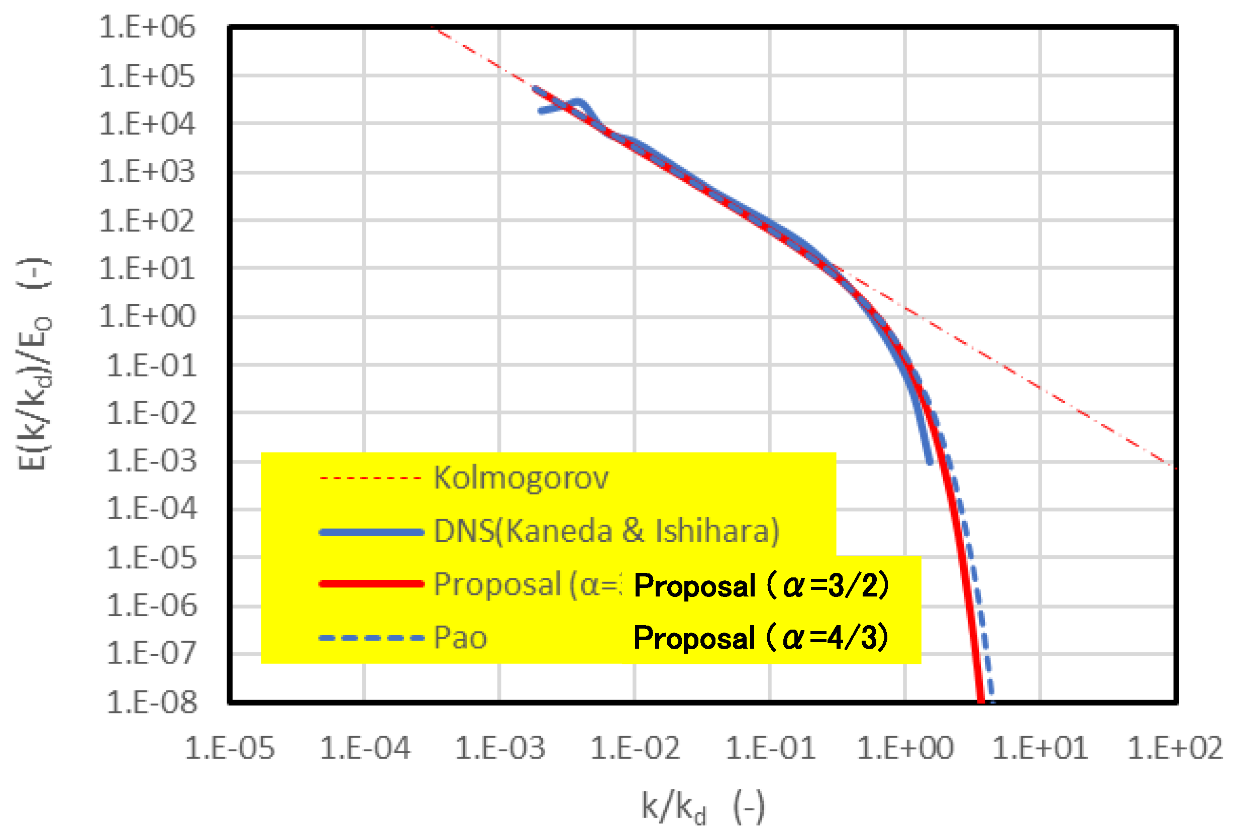
Ishihara et al. performed direct numerical simulations (DNS) of isotropic turbulence up to ${2048}^3$ grid points at $R{e}_{\lambda }=433$, and subsequently Kaneda and Ishihara extended the resolution to ${4096}^3$ at $R{e}_{\lambda }=675$ (Ishihara et al., 2009; Kaneda & Ishihara, 2006). The energy spectra reported by Ishihara et al. exhibit a $-5/3$ power law in the inertial subrange (corresponding to the blue curve in Figure 1) and an exponential-type decay in the dissipation range.

In these DNS datasets, the effective resolution in $k/k_d$ reaches at most approximately $\sim 3$. Under this context, Figure 1 compares the DNS energy spectrum obtained with ${2048}^3$ grid points at $R{e}_{\lambda }=433$ against the spectrum predicted by the present model. In this study, we use $C_K=1.5$as stated above. The proposed model (red curve in the figure) reproduces, with high accuracy, the spectral characteristics observed in DNS across both the inertial and dissipation ranges. For reference, we also plot the Pao model corresponding to $m={\displaystyle \frac{4}{3}}$ within the present formulation; however, the Pao model tends to overestimate the energy spectrum in the dissipation range relative to the DNS results. These comparisons support the plausibility of the exponent range evaluated in this Section. The same comparison has also been noted by Hebishima and Inage (2025).

5.8. Summary: Connecting the First and Second Stages

We summarize the conclusions of this Section. In the first stage (the dynamical level), within the framework of an autonomous conservative FP semigroup, the relative turbulence entropy becomes a Lyapunov functional, and

${\displaystyle \frac{d}{dt}}{S}_{\mathrm{r}\mathrm{e}\mathrm{l}}\left(t\right)=\sigma \left(t\right)\ge 0,$ (205)

holds rigorously. In contrast, in the second stage (the selection level), the WKB analysis in Section 4 constrains the dissipation tail to the stretched-exponential form

$E\left(k\right)\sim C\hspace{0.17em}{\epsilon }^{2/3}\hspace{0.17em}{k}^{-5/3}\mathrm{e}\mathrm{x}\mathrm{p}\left[-\beta {\left({\displaystyle \frac{k}{k_d}}\right)}^m\right],$ (179)

together with the coupling relation

$m=1+{\displaystyle \frac{\gamma }{2}}.$ (180)

Accordingly, we construct the reference distribution $P_s^{\left(\gamma \right)}\left(\xi \right)$ globally on $\left.\mathsf{\Omega }=[{\xi }_{-},\mathrm{\infty }\right)$ and, based on

$P_s^{\left(\gamma \right)}\left(\xi \right)={\displaystyle \frac{C_s^{\left(\gamma \right)}}{D^{\left(\gamma \right)}\left(\xi \right)}}\mathrm{e}\mathrm{x}\mathrm{p}\left({\int }^{\xi }{\displaystyle \frac{A^{\left(\gamma \right)}\left(\eta \right)}{D^{\left(\gamma \right)}\left(\eta \right)}}\hspace{0.17em}d\eta \right), (\xi \in [{\xi }_{-},\mathrm{\infty }\left)\right),$ (241)-(243)

define the one-dimensional optimization (minimization of the KL distance $D\left(\gamma \right)$)

${\gamma }^{*}\in \mathrm{a}\mathrm{r}\mathrm{g}\underset{\gamma \in \mathsf{\Gamma }}{\mathrm{m}\mathrm{i}\mathrm{n}}{\int }_{{\xi }_{-}}^{\mathrm{\infty }}{P}_{\gamma }\left(\xi \right)\mathrm{l}\mathrm{n}\left({\displaystyle \frac{P_{\gamma }\left(\xi \right)}{P_s^{\left(\gamma \right)}\left(\xi \right)}}\right)\hspace{0.17em}d\xi .$ (269)

Then $m$is not fixed externally, but is identified as

$m^{*}=1+{\displaystyle \frac{{\gamma }^{*}}{2}}.$ (270)

Thus, the exponent $m$in this paper is not an a posteriori fitting parameter, but is positioned on a verifiable chain of logic:

$(\mathrm{irreversibility}: \mathrm{H}-\mathrm{theorem}) \Rightarrow (\mathrm{dissipation} \mathrm{tail}: \mathrm{WKB}) \Rightarrow (\mathrm{global} \mathrm{physical} \mathrm{domain}: \mathsf{\Omega }=[{\xi }_{-},\mathrm{\infty })) \Rightarrow (\mathrm{one}-\mathrm{dimensional} \mathrm{optimization} \mathrm{in} \gamma ).$

6. Conclusions

This study established a two-level theory—obtained by serially connecting a dynamical coarse-graining based on the spectral equation of three-dimensional homogeneous isotropic turbulence (the Lin equation) and an information principle in logarithmic wavenumber space (a reduced MaxEnt principle)—and thereby positioned the dissipation-range spectral shape (in particular, the stretched-exponential tail) not as an ad hoc fit, but as the outcome of a verifiable logical chain.

The main achievements can be summarized in the following three points.

• Stage 1 (dynamical level): autonomous FP semigroup and H-theorem.

We explicitly formulated a one-dimensional Fokker–Planck description on the logarithmic wavenumber $\xi =\mathrm{l}\mathrm{n}k$ as an autonomous time evolution (a semigroup). By showing that the relative turbulence entropy (the sign-reversed KL distance) is a Lyapunov functional with monotonicity, we mathematically fixed the “arrow of time” in scale space.

2.

Stage 1.5 (asymptotic constraint): admissible class via WKB.

By applying WKB analysis to the stationary equation in the dissipation range, we clarified that the tail becomes stretched exponential and that the admissible range of exponents is constrained (under asymptotic coefficient scaling). Moreover, the WKB coupling provides the constraint $m=1+\gamma /2$, which reorganizes the degrees of freedom and directly leads to the final formulation in Section 5.

3.

Stage 2: removing arbitrariness and one-dimensional Hyper-MaxEnt.

To eliminate the largest potential arbitrariness—leaving $\beta$ free—we fixed $\beta =\beta \left(m\right)$ by enforcing dissipation-rate consistency, thereby reducing the freedom to $m$ alone. In addition, we unified the lower integration bound for the dissipation-rate integral to ${\xi }_{-}$ (equivalently $k_f$) and closed the remaining “mathematical gaps” concerning integrability and well-definedness of the KL functional. As a result, the selection problem closes as a one-dimensional optimization (Hyper-MaxEnt), and the exponent $m^{*}$can be defined as the exponent within the admissible set that minimizes the KL distance to the reference distribution.

In one sentence, the conclusion of this theory is as follows: the dissipation-range exponent $m$ is selected as $m^{*}$ by necessity from (i) the convergence structure permitted by the dynamics (H-theorem), (ii) the tail class constrained by WKB asymptotics, and (iii) an information principle (reduced MaxEnt) after removing arbitrariness by dissipation-rate consistency.

Natural next steps include: (a) calibration of the reference-distribution parameters from DNS/experiments and robustness assessment of $m^{*}$; (b) extensions to incorporate finite-$Re$ effects, nonstationary forcing, and nonlocality (including identification of FP coefficients and refinement of boundary conditions); and (c) generalization to scalar mixing and anisotropic turbulence. These directions can be pursued in a verifiable manner while preserving the core structure of the present framework—“dynamics $\to$asymptotics $\to$information.”

References

- Kolmogorov, A. N. The local structure of turbulence in incompressible viscous fluid for very large Reynolds numbers. Doklady Akademii Nauk SSSR 1941, Vol. 30, 301–305. [Google Scholar] [CrossRef]
- Batchelor, G. K. The Theory of Homogeneous Turbulence; Cambridge University Press, 1953. [Google Scholar]
- Frisch, U. Turbulence: The Legacy of A. N. Kolmogorov; Cambridge University Press, 1995. [Google Scholar]
- Pope, S. B. Turbulent Flows; Cambridge University Press, 2000. [Google Scholar]
- Davidson, P. A. Turbulence: An Introduction for Scientists and Engineers, 2nd ed.; Oxford University Press, 2015. [Google Scholar]
- Sagaut, P.; Cambon, C. Homogeneous Turbulence Dynamics, 2nd ed.; Springer, 2018. [Google Scholar]
- Pao, Y. H. Structure of turbulent velocity and scalar fields at large wavenumbers. Physics of Fluids 1965, Vol. 8(No. 6), 1063–1075. [Google Scholar] [CrossRef]
- McComb, W. D.; Yoffe, S. R. Renormalization-group methods for Navier–Stokes turbulence. Journal of Physics A: Mathematical and Theoretical 2017, Vol. 50, 415501. [Google Scholar]
- Zhou, Y. Turbulence theories and statistical closure approaches. Physics Reports 2021, Vol. 935, 1–117. [Google Scholar] [CrossRef]
- Verma, M. K.; Kumar, A.; Kumar, P.; Barman, S.; Chatterjee, A. G.; Samtaney, R.; Stepanov, R. A. Energy spectra and fluxes in dissipation range of turbulent and laminar flows. Fluid Dynamics 2018, Vol. 53(No. 6), 862–873. [Google Scholar] [CrossRef]
- Buaria, D.; Sreenivasan, K. R. Dissipation range of the energy spectrum in high Reynolds number turbulence. Physical Review Fluids 2020, Vol. 5, 092601(R). [Google Scholar] [CrossRef]
- Gorbunova, A.; Balarac, G.; Canet, L.; Eyink, G.; Rossetto, V. Spatio-temporal correlations in three-dimensional homogeneous and isotropic turbulence. Physics of Fluids 2021, Vol. 33, 045114. [Google Scholar] [CrossRef]
- Solsvik, J.; Jakobsen, H. A. Development and application of population balance models for dispersed turbulent two-phase flow: A review. AIChE Journal 2016, Vol. 62(No. 6), 1933–1953. [Google Scholar]
- Solsvik, J.; Jakobsen, H. A. Development of fluid particle breakup and coalescence closure models for the complete energy spectrum of isotropic turbulence. Industrial & Engineering Chemistry Research 2016, Vol. 55(No. 23), 6201–6230. [Google Scholar]
- Tanogami, T.; Araki, K. Information-thermodynamic structure of the turbulent energy cascade. Physical Review Research 2024, Vol. 6, 043261. [Google Scholar] [CrossRef]
- Kraichnan, R. H. The Structure of Isotropic Turbulence at Very High Reynolds Numbers. Journal of Fluid Mechanics 1959, 5, 497–543. [Google Scholar] [CrossRef]
- Kovasznay, L. S. G. Spectrum of Locally Isotropic Turbulence. Journal of the Aeronautical Sciences 1948, 15(12), 745–753. [Google Scholar] [CrossRef]
- Verma, M. K. Energy Transfers in Fluid Flows: Multiscale and Spectral Perspectives; Cambridge University Press: Cambridge, 2019. [Google Scholar]
- Risken, H. The Fokker–Planck Equation: Methods of Solution and Applications, 2nd ed.; Springer: Berlin, 1996. [Google Scholar]
- Gardiner, C. W. Stochastic Methods: A Handbook for the Natural and Social Sciences, 4th ed.; Springer: Berlin, 2009. [Google Scholar]
- Cover, T. M.; Thomas, J. A. Elements of Information Theory, 2nd ed.; Wiley: New York, 2006. [Google Scholar]
- Jaynes, E. T. Information Theory and Statistical Mechanics. Physical Review 1957, 106, 620–630. [Google Scholar] [CrossRef]
- Jaynes, E. T. The Minimum Entropy Production Principle. Annual Review of Physical Chemistry 1980, 31, 579–601. [Google Scholar] [CrossRef]
- Pressé, S.; Ghosh, K.; Lee, J.; Dill, K. A. Principles of Maximum Entropy and Maximum Caliber in Statistical Physics. Reviews of Modern Physics 2013, 85(3), 1115–1141. [Google Scholar] [CrossRef]
- Prigogine, I. Introduction to the Thermodynamics of Irreversible Processes, 3rd ed.; Wiley: New York, 1967. [Google Scholar]
- Seifert, U. Stochastic Thermodynamics, Fluctuation Theorems and Molecular Machines. Reports on Progress in Physics 2012, 75, 126001. [Google Scholar] [CrossRef] [PubMed]
- Olver, F. W. J. Asymptotics and Special Functions; Academic Press: New York, 1974. [Google Scholar]
- Bender, C. M.; Orszag, S. A. Advanced Mathematical Methods for Scientists and Engineers; McGraw–Hill: New York, 1978. [Google Scholar]
- Hinch, E. J. Perturbation Methods; Cambridge University Press: Cambridge, 1991. [Google Scholar]
- Spohn, H. Entropy Production for Quantum Dynamical Semigroups. Journal of Mathematical Physics 1978, 19, 1227–1230. [Google Scholar] [CrossRef]
- Van Kampen, N. G. Stochastic Processes in Physics and Chemistry, 3rd ed.; North-Holland: Amsterdam, 2007. [Google Scholar]
- de Groot, S. R.; Mazur, P. Non-Equilibrium Thermodynamics; Dover, New York, 1984. [Google Scholar]
- Kullback, S.; Leibler, R. A. On Information and Sufficiency. Annals of Mathematical Statistics 1951, Vol. 22(No. 1), 79–86. [Google Scholar] [CrossRef]
- Kullback, S. Information Theory and Statistics; Wiley: New York, 1959. [Google Scholar]
- Lebowitz, J. L.; Spohn, H. A Gallavotti–Cohen-Type Symmetry in the Large Deviation Functional for Stochastic Dynamics. Journal of Statistical Physics 1999, Vol. 95(Nos. 1–2), 333–365. [Google Scholar] [CrossRef]
- Edwards, S. F.; McComb, W. D. Generalized Taylor–Kármán Momentum Transfer Theory of Isotropic Turbulence. Journal of Physics A: General Physics 1969, Vol. 2(No. 2), 157–171. [Google Scholar] [CrossRef]
- Verma, M. K.; Chatterjee, A. G. An Introduction to Multiscale Analysis in Turbulence; Springer: Singapore, 2022. [Google Scholar]
- Ishihara, T.; Gotoh, T.; Kaneda, Y. Study of High–Reynolds Number Isotropic Turbulence by Direct Numerical Simulation. Annu. Rev. Fluid Mech. 2009, 41, 165–180. [Google Scholar] [CrossRef]
- Kaneda, Y; Ishihara, T. High-resolution direct numerical simulation of turbulence. J Turbul 2006, 7(20). [Google Scholar] [CrossRef]
- Hebishima, H.; Inage, H. A unified turbulence model bridging low and high Reynolds numbers: Integrating shell models with two-scale direct interaction approximation. Chaos, Solitons and Fractals 2025, 198, 116535. [Google Scholar] [CrossRef]
Figure 1.
This figure compares the energy spectrum obtained from the proposed model with that from direct numerical simulation of turbulence.
Disclaimer/Publisher’s Note: The statements, opinions and data contained in all publications are solely those of the individual author(s) and contributor(s) and not of MDPI and/or the editor(s). MDPI and/or the editor(s) disclaim responsibility for any injury to people or property resulting from any ideas, methods, instructions or products referred to in the content. |
© 2026 by the authors. Licensee MDPI, Basel, Switzerland. This article is an open access article distributed under the terms and conditions of the Creative Commons Attribution (CC BY) license (http://creativecommons.org/licenses/by/4.0/).
Copyright: This open access article is published under a Creative Commons CC BY 4.0 license, which permit the free download, distribution, and reuse, provided that the author and preprint are cited in any reuse.