
Submitted:
05 January 2026
Posted:
06 January 2026
You are already at the latest version
Abstract
In this paper, we consider the development of last scattering polarization from the point of view of our new model of structure formation. It has long been accepted that the CMB polarization on a 1° scale is a consequence of Thomson scattering at the tail-end of the epoch of recombination. We present a new simulation that confirms that idea, but we also show that the standard model, which is based on acoustic oscillations, of how this came about, is unworkable for several reasons in spite of its general acceptance. Our new model of structure formation argues that all structures came into existence at a time of about 10^-5 s and that they did so containing a high density of photons. These were initially trapped inside the structure by scattering, but later began to flow out of the structure with the onset of recombination, and it was this radial flow that created the asymmetric condition necessary for the development of the polarization. Our simulation shows that this radial flow acquired a high degree of polarization in the transverse direction which was then diluted by the background CMB radiation to yield the small degree of polarization detected by observers.
Keywords:
CMB polarization
; last scattering
; CMB anisotorpies
; cosmic structure formation
1. Introduction
There were two epochs in the evolution of the universe during which the polarization of the CMB was established. The first was the relatively short “last scattering” period that concluded the era of recombination. The polarization created during this era has an angular scale of 1°, which matches the angular size of the superclusters of that time. Much later, beginning at the time of galaxy formation, a second period of CMB polarization began after radiation created by supermassive black holes re-ionized the neutral hydrogen that filled the universe. Thomson scattering was again possible, leading to additional CMB polarization, this time on angular scales of 5° or more, corresponding again to the angular size of superclusters. This era had no definite ending, as did the last scattering epoch, but instead the scattering faded away as both the photon and electron densities decreased with the expansion of the universe.
The study of the CMB polarization has a long history, with most, if not all, developments being based on the idea that cosmic structures are a consequence of small perturbations in the initial distribution of matter that eventually grew by accretion into the structures we see today (See e.g. [1,2,3,4,5]). During the past few years, we have been developing a totally different model of structure formation in which all structures in proto form came into existence simultaneously at the time of nucleosynthesis with all their present-day matter content, and with initial sizes several times larger than their present-day sizes. Together with their matter content, the structures also acquired a high density of photons that eventually became today’s CMB [6,7]. The standard model supposes that the CMB temperature and polarization anisotropies came into existence simultaneously during the epoch of last scattering [5]. According to this new model, while that is true of the polarization, the temperature anisotropies were built in at the time of nucleosynthesis.
The general idea of last scattering polarization can be broken down into just a couple of ideas. First, Thomson scattering of a flow of photons traveling in a single direction will result in photons preferentially traveling away from the scatterings in directions perpendicular to the incoming flow, with a net polarization also normal to the incoming flow. If, on the other hand, the intensity of the incoming flow is symmetric or random, the net polarization seen by an observer will be zero because the polarizations of the individual photons will average out. The second idea is that, once a population of photons has acquired a net polarization, the scattering of those photons must cease because any significant amount of additional scattering will randomize their polarizations thus eliminating the net polarization.
It follows that any theory of polarization must explain the origin of the photons, why their distribution was asymmetric, and why the scattering ceased. Everyone will agree that the scattering ceased at the time of recombination because the expansion of the universe cooled the photons to the point that the free electrons could bind with free protons to form neutral hydrogen. In cosmic terms, this process happened quickly, but still it was a matter of more than 500,000 years. Our ideas about the origin of the photons with their asymmetric flow are where we differ completely from the standard model.
Even though the standard model based on the existence of acoustic oscillations is widely accepted, we will argue that, on the scales necessary to explain the 1° scale of the polarization, it is unworkable. The standard model idea is that the universe was filled initially with an isotropic distribution of radiation that together with free electrons initiated acoustic oscillations whose peaks and troughs induced asymmetric flows as the photons travelled from the hot to the cold regions [1].
One problem with this idea is that the 1° scale of the polarization, which corresponds to the size of superclusters of the time, would require coordinated crests and troughs on a scale of . There is no preferred origin or direction so each point in space would receive waves from sources on a shell with a radius of , where is the sound speed, while the sizes of the sources could not have been larger that . Comparing the area of the sphere with the size of the sources shows that each point in space would be receiving input from about uncorrelated sources which would add up to some mean value with a large variance rather than something with crests and troughs in a definite direction. As we showed in [8], considerations of the energy required to explain the temperature anisotropies also result in a similar number of uncorrelated sources. To account for not just the waves but also for the cosmic web, a different collection of sources for every point would have needed to conspire all across the universe to make this happen.
Another problem with the standard model idea is that it assumes the existence of gravitationally induced forces that are necessary for the existence of the waves. While gravitation would have had consequences on length scales on the order of a few lightyears or less at the time of last scattering, we proved in [9] that on any larger scale, the expansion of the universe completely overwhelmed any possible gravitational interaction. The particles were moving away from each other far too rapidly for gravity to influence their motion. So, while oscillations might have been possible on small scales, the gravitationally-induced pressure differences necessary for oscillations on scales the size of superclusters could not have existed before recombination, if ever. Even on scales as small as a galaxy, it would have been long after the time of recombination before gravity began to have any effect.
The standard model idea is that initial events at one place created a flow of matter and radiation that eventually coalesces into structures somewhere else far away. In our new model, there was no such movement. Our model is described in several of our publications, and is summarized in [6], so we will only present a brief introduction of the relevant portions of the model here. In this model, the universe began with a Planck-era inflation during which a self-organizing fractal imprint was established in the vacuum. After the inflation had ended and causality was in play, Einstein’s equations described the evolution of the universe. The basis of our new model is the observation that the curvature of the vacuum must vary with time, and that the vacuum energy must be included in the energy-momentum tensor. We have found the exact solution of Einstein’s equations for such a universe, which gives a scaling that demands an exponential acceleration of the present-day expansion. The formula for the scaling is
where the two adjustable parameters are and with , . The vacuum energy and pressure are given by
and the total energy, given by the sum
The additional, none adjustable, parameters in these formulas are fixed by the solution to be and .
This model makes a number of predictions that agree with observations. For one, the calculated luminosity distance matches the measurements over the whole range of redshifts [6]. For another, its prediction of the present-day vacuum energy density () is within a factor of 3 of the accepted value of the dark energy density. Our energy-momentum tensor does not contain a cosmological constant, but both the energy and pressure formulas contain a constant term which gives their respective values at infinite time. Because these have opposite signs, they cancel in the total energy sum. We can, however, rewrite the energy-momentum tensor in terms of energy and pressure variables that vanish at infinite time, and with that change, the tensor does contain a constant whose value is
which is exactly the same as the cosmological constant’s value of ,10]. We emphise that Equation (4) is a formula, not a parameter fit, which resolves the long-standing mystery about the origin of the cosmological constant’s value.
The model predicts that, at the time of nucleosynthesis, the vacuum energy density was about 11 orders of magnitude larger than the matter energy density. It also predicts that the present-day vacuum energy density is be about the same as that of the matter energy density, and the two together resolve the so-called coincidence problem.
Recently, the DESI collaboration has hinted that dark energy might be varying with time. Our model does not contain dark energy in the standard model, sense, but our vacuum energy does vary with time and our Equation (3) tells by how much. In the limit of infinite time, the equation-of-state, although this is a standard model concept which doesn’t appear in this new model.
This model solves a more fundamental problem presented by the standard model concept of a cosmological constant that exists as a distinct entity. Introducing such a constant in Einstein’s equations presents no problem, but the fact is that the vacuum has no means by which to express such a phenomenon. The universe unfolds as a sequence of hyperspheres with the expansion occurring at each spatial point simultaneously. The critical point is that each such point has a spacelike separation from every other point, so each point must evolve without any knowledge of what any other point is doing. For the vacuum to express a cosmological constant, on the other hand, each point would have to know what every other point was doing to express the same value for the constant, and that is impossible. Our new model avoids the concept of an independent cosmological constant and speaks instead of time-varying energy and pressure with each having a non-zero infinite-time limit whose predicted value is the same as the standard model cosmological constant. Our model is local. With time-varying curvature acting on itself, Einstein’s equations impose the constraint that the curvature must be proportional to the energy density, and to maintain that proportionality, the vacuum must expand. Ignoring the effects of matter, which were extremely small in the early universe, each point arrives independently at the same values for the acceleration, and the energy and pressure including their values at infinite time.
We remind the reader that all these results are the consequence of just two ideas, 1) thatthe curvature varies with time, and 2) that the vacuum energy must be included in the energy-momentum tensor.
Getting back to structures, at a time of about , in a process regulated by the inflation era vacuum imprint, a very small percentage of the energy of the vacuum underwent neutron/antineutron pair production with about extra neutrons for every pair. The masses of the proto-structures were then fixed, but their initial sizes were much larger than their final, present-day sizes in present-day terms1. A byproduct of this process was that the structures ended up containing a very high density of radiation created by both baryon annihilation and charge exchange reactions. It was this radiation that became the CMB with its temperature anisotropies built in.
In Figure 1, we show the evolution of a galaxy cluster predicted by this model [9]. Each line represents the evolution of an evenly spaced interior shell of the cluster. There is no hint in the curves that gravity has any effect on the evolution of structures until long after the epoch of last scattering. Note that this model predicts that the galaxy cluster reached in final size at a time of about or a redshift of about 7. This model also predicts that all galaxies reached their final state at the same time, and that they all developed supermassive black holes because they would have otherwise undergone free-fall collapse and ceased to exist. Both these predictions are in perfect agreement with the results coming from the JWST which is seeing fully developed massive galaxies at a time too early to be accounted for accretion models of structure formation.
Focusing now on polarization, superclusters at the time of last scattering were much smaller than they are now, and looking back at them from the present, we find their apparent size to be about 1° which matches the characteristic angular size of the measured polarization. That is compelling evidence that superclusters were, in some way, responsible for the polarization. But superclusters are made up of one or more galaxy clusters arranged in filaments, so we really need to concentrate on objects the size of galaxy clusters. The present-day diameter of galaxy clusters is about 5% of the linear dimension of a supercluster, but according to our model, at the time of last scattering, the proto-galaxy clusters were nearly 10 times larger, so superclusters at that time would appear more like blobs than filaments. This is shown in Figure 2 from the Planck satellite results [11].
It is reasonable, then, to suppose that the proto-galaxy clusters of each supercluster were collectively responsible for the polarization.
2. The Simulation Model
The basis of our study will be an idealized spherically symmetric galaxy cluster with the mass and present-day size of the Virgo Cluster. Henceforth, we will refer to the sphere as the cluster. We fill this cluster with photons and electrons in amounts fixed by our model, and then watch what happens using a Monte Carlo approach. In the displayed results, dimensions are scaled by the present-day size of the Virgo cluster (), and times are cosmic times expressed in seconds.
To build the model, we divide the cluster into a series of concentric shells of equal thickness and assign to each a distribution of electrons fixed by an assumed radial matter distribution. An example distribution is shown in Figure 3.
The normalization of the curve is fixed by our model requirement that the average density of the cluster should be 2.5 times greater than the energy density of the vacuum, and that its radius is 7.8 times larger than its present-day size, [9]. We fill each shell of the cluster with the primordial blackbody photons with a distribution determined by assuming that their number density is proportional to the matter number density [7]. Their temperature profile is then given by the usual blackbody formula, which at the outer boundary equals the time-varying CMB background temperature.
We also define a so-called outside shell, which begins at the outer boundary of the cluster and extends to the location of the escaped photon furthest from the center of the cluster so its size varies with time. The term “escaped” will be explained below.
The electrons are assumed to be stationary, so they remain within whichever shell they originally occupied. Their densities decrease, however, both because of the expansion and as a result of recombination. To model the latter, we used the curve shown in Figure 4 from [12], which gives the recombination depletion in terms of redshift. The actual depletion is a function of the temperature, so we converted to temperature using the FRW scaling model (instead of our new model scaling.)
This curve defines a temperature-dependent range of times for each shell during which the electron fraction drops from 1 to some small number. In what follows, we will use the term, to indicate the earliest time at which the electron fraction of any shell dropped below . Similarly, we define to be the last time any shell’s fraction dropped below . Finally, by we refer to the time that the background CMB temperature dropped to . Note later that because our scaling is different from the standard model scaling, these events occurred earlier in time than they do according to that model.
We run the simulations in two phases. During the first, we ignore the polarization. We fix the dynamic temperature of each of the shells using a method to be described shortly, and then use those temperature distributions along with the instantaneous densities of the electrons to determine the photon mean-free-paths (MFP) for each shell as a function of time.
Because the number of actual photons is astronomically large, we use the Monte Carlo method of following the evolution of a manageable number of proxy “photons” which, in this phase, we call “cmbs”. Each of these is characterized by a blackbody spectrum whose temperature varies with the expansion and scattering, but not by a polarization. We save the calculated shell dimensions and MFPs from each run for later use in the second phase.
In the second phase, we again fill the same cluster with simulation photons, but this time each “fton” is a proxy for any one of a huge number of single linearly-polarized photons. We start each simulation well before the onset of last scattering at a time when the scattering rate is high enough to eliminate any net polarization. This allows us to initialize the ftons with random polarizations, but from then on, their polarizations are determined by the scattering events.
3. First Phase – Expansion, Temperatures, Mean-free-paths, etc.
We start by assigning some number of cmbs to the outermost cluster shell, which we will call the outer shell (not to be confused with the outside shell), and then filling the remaining shells with counts in proportion to their densities fixed by the temperatures of the shells as described above. Each cmb is assigned a random position and direction within its shell, and its temperature is set to the temperature of its shell.
Initially, the outside shell is empty of cmbs. It is, however, full of background photons which contribute indirectly. First, these determine the MFP of the cmbs that escape the cluster, and second, they are the source of the photons that enter the cluster from outside over time. During each time cycle, the outside shell fills a shell of thickness immediately outside the boundary of the cluster with potential cmbs that are assigned random positions and directions. The distance is the maximum distance that a cmb could travel during a single time step. We then allow each to move in its assigned direction. Depending on the current MFPs, some of these will cross the boundary into the cluster. Those that do are said to have been injected. They become cmbs and are lumped together with all the other cmbs. Those that didn’t cross the boundary are dumped.
As the simulation progresses, some cmbs will cross from inside the cluster into the outside shell, and are then deemed to have escaped. Most of these will move away from the cluster, but because of scattering, some will cross back into the cluster and are then deemed to have been captured. As mentioned earlier, the outer boundary of the outside shell is fixed at any time by the position of the escaped cmb furthest from the boundary of the cluster.
The simulation proceeds by cycling through a series of steps. The origin of our system is the center of the cluster, and expansion is relative to that center. Each cycle begins with an expansion step in which the radii of the shells, the cmb’s distance from the center of the cluster, and their temperatures are adjusted for the change in the scaling. The temperature of the outside shell is set to , and all cmbs within the outside shell are identified. In the third step, the average blackbody temperature of each shell is calculated by adding the energies of all the cmbs that happen to be inside that shell, and then using the standard blackbody energy formula to get the temperature. Using this temperature and the current density of the electrons, the MFP of each shell is calculated. The scattering rate per cmb is given by the formula,
where is the density of free electrons. We get the latter from the expansion of the shells together with the recombination curve of Figure 3. The MFP is then given by .
We next compare the MFP of each shell with the thickness of the shells. If the MFP is less than the thickness, we assume that the scattering rate is high enough to thermalize the cmbs of that shell, and each is assigned the average temperature of the shell. Otherwise, the cmb temperatures within the shell remain unchanged during that time cycle
Next, the outside shell performs the injection process outlined above. This process results in a minor amount of cooling of the interior of the cluster, but a significant increase in the total number of cmbs after the end of scattering.
The final step is the heart of the process. Looping over all the cmbs, we advance each cmb’s position by a series of sub-steps until the length of its travel either reaches in which case, it didn’t scatter during that time step, or it uses up its “distance-to-scatter”, explained below, in which case it does scatter. Because the cmb energies are much smaller than the electron mass, the scattering occurs with no loss of energy by the cmb (Thomson scattering). After a cmb scatters, because each represents a huge number of actual photons, there will not be a preferred direction, so we choose a new random direction from a uniform distribution of possible angles. At the same time, the cmb is assigned a new distance-to-scatter equal to the MFP at its current position. At time advances, the distance-to-scatter is corrected for the expansion of the universe, and for changes in the MFP as the cmb moves from one shell to another. It is then reduced by the distance each cmb travels during the following time steps until it hits zero, whereupon the cmb scatters.
We will now show some results. We divided the cluster into 30 shells and set the initial cmb count in the outer shell to be 4000, which results in a total initial cmb count of 79,300.
In Figure 5, we show the last scattering ranges for each of 30 shells. The shell durations are much the same, but the ranges are spaced in time, with the outermost shell beginning first because it has the lowest temperature. These curves illustrate the meaning of the times of last scattering start and end.
In Figure 6, we show the resulting MFPs for the innermost shell, the outermost shell, and the shell whose index is in the middle. The MFPs increase from the inside to the outside for a given time.
There are several curves in this figure. The causality curve is a plot of measured from the center of the cluster with a start time of . The green line indicates the common thickness of the shells, which increases because of the expansion. The curved lines are the MFPs. The blue lines were computed assuming that the temperatures of shells were determined solely by the expansion of the universe, while the red curves are the MFPs calculated during the simulation using the method discussed earlier. We see that the curves are identical up until the time, . Before , the MFPs were much smaller than the shell thickness, and, as we will see, the cmbs remained trapped in their original shells. In particular, almost no cmbs crossed the cluster boundary in either direction. After that time, the MFPs underwent a rapid increase in magnitude as the free election fraction dropped. The MFPs soon became larger than the shell thickness, and the cmbs began to move between shells and to leave the cluster. Eventually, the free election fraction dropped to zero, and the MFPs became infinite.
As the temperature dropped, the photons eventually reached the point that their probability of an additional scattering vanished. In Figure 7, we show the time intervals for each shell during which the number of scatterings per cmb dropped from 1.05 to 0.95. In this figure, shell 30 is the outside shell.
In Figure 8, we show the total number of scatters as a function of time. We see that the total number of scatters was high before the free election fraction began to fall. The change was initially gradual, but then it dropped dramatically soon after .
The sharp peak in the curve is not physical, but it isn’t an error either. At the time of the elbow in the curve, a significant number of cmbs had their last scattering. The code records a scattering when a cmb uses up is allotted distance-to-scatter. The peak is simply the point at which the cmbs that last scattered at the elbow did just that. By the time of , the MFPs had become infinite, and scattering had ceased.
In Figure 9, we show the number densities of the cmbs versus distance from the cluster center. Each curve represents a single time, and in this case, the curves were spaced 15 simulation cycles apart.
It is clear that as time increased, the densities decreased, and the cmbs spread out. Starting at the top, the blue curves show the distributions before the beginning of the last scattering epoch. Notice the vertical tails on each of those curves. Those show the number densities in the outside shell, the thickness of which is fixed by the location of the escaped cmb furthest from the center. The line is vertical because during this epoch, the cmbs were trapped in the cluster by the scattering.
The green curves show the distributions within the last scattering epoch. The changing slope of the outside shell tail shows that cmbs are escaping and moving away from the cluster in increasing numbers. Finally, the red curves show the progression of the distribution after the end of the last scattering. By the time of the first red curve, the total count of cmbs had increased to 350,000, of which 87% were outside the cluster.
Before the onset of the last scattering epoch, the number of injected cmbs was minimal because the scattering within the cluster that kept the cmbs inside also kept the potential injected cmbs out. After the onset of last scattering, the injection rate rapidly increased, resulting in an increasing number of captured cmbs. Eventually, when scattering ceased, the cluster became transparent. The remaining captured cmbs escaped, and they continued to do so as the outside shell continued to inject more cmbs.
Finally, in Figure 10, we show the temperature distributions.
This is less dramatic than the previous figure. We see that there was a stable distribution before the onset of last scattering in which the temperatures only changed as a result of the expansion. After the onset of last scattering, the cluster shells also began to lose energy because of the escaping cmbs carried away energy, and by the time of the last displayed curve, whose time is , the distribution was flat with a temperature close to the CMB background temperature.
In the next two figures, we show the final time distribution curve in detail. This distribution’s total count of escaped cmbs was on the order of 450,000, whereas the initial population of cmbs was on the order of 80,000, all of which were initially in the interior of the structure. To convert that ensemble into something manageable, we sorted the cmbs into a series of bins of width, or . In Figure 11, we show the counts of escaped cmbs grouped by whether or not each cmb underwent at least one scattering at some point in the past. The red curve shows those with scattering and the green, those without. The heavy blue line at the bottom of the figure indicates the radius of the cluster, and the heavy red line indicates the extent of the outside shell. The cutoff at the boundary of the cluster reflects the fact that we are only considering escaped cmbs.
The FWHM is about 10 bins, which is somewhat larger than the diameter of the Virgo proto-cluster adjusted for the scaling and the multiplier of 7.8. (Compare the heavy blue line at the bottom of the graph with the width of the peak.) It is apparent that the “with scatter” cmbs are traveling ahead of the “no scatter” cmbs, which reflects the fact that a large portion of the “no scatter” cmbs had to have entered the structure after the last scattering and then pass through some portion of the cluster before escaping.
In Figure 12, we show the temperature-CMB ratio, this time with a linear scale.
The blue curve was obtained by combining the “no scatter” with the “with scatter” cmbs to show the effect of the dilution. As time advances, the peaks move to the right as they radiate away from the cluster.
What you undoubtedly notice from this figure is that the predicted temperature anisotropy is orders of magnitude larger than the observed anisotropies. It is not that our calculated anisotropy is wrong; it is that we have not yet allowed for the dilution of the anisotropies by the background CMB photons that fill space, or the finite resolution of the telescopes used to detect the anisotropies. The result with these included is shown in Figure 13 taken from [13].
In this figure, we show the peak temperature fraction () as a function of time for a single position, so an observer would see the curves moving past his or her location from right to left. The observer would see a rapid initial increase in the temperature followed by a slow decline. The upper curve is what one would observe with a telescope with perfect resolution, and without dilution. The lower two curves include the dilution by the background CMB radiation, the degree of which is dependent on the resolution of the telescopes. The horizontal lines show the peak anisotropy temperatures recorded by the Planck and WMAP telescopes. The model predictions are very close to the observed values.
We have explored the origin of the CMB temperature anisotropies, and we have calculated the dimensions and MFPs of each of the shells as a function of time. We now move on to the polarization.
4. Second Phase - Polarization
In the second phase, we switch to a collection of proxy photons called ftons, which are considered to be single objects rather than collections. Instead of being characterized by a temperature, ftons are characterized by their polarization. We set up the simulation in parallel with the first phase, except that the ftons are initialized with a random linear polarization instead of a temperature. The simulation proceeds as before except that we now use the previously calculated MFPs.
The one significant difference is how we treat the scattering. In the cmb case, because each represented a huge number of actual photons, the direction after the scattering was randomly selected from a uniform distribution of possible angles. In the fton case, because we are dealing with individual proxy photons, we again assign a random post-scatter direction, but this time, from a non-uniform distribution proportional to the Thomson scattering cross section,
where is the angle between the incident polarization and the direction of the outgoing photon. Scatterings with near are more likely to occur than those with small values of . To create a corresponding biased probability distribution, we used the simple method of dividing the range of into a set of bins, and then creating a list of duplicate values with the count of duplicate bins added for each value of proportional to . Thus, the value will not appear in the list at all, and the value will appear in the list more often than any other value. To obtain a random , we use a uniform random number generator to pick a list index with being the value held by the bin at that index. Once is determined, we then assign an azimuthal angle in the range 0 to , assuming a uniform distribution. With the outgoing direction established, the polarization of the outgoing fton is fixed by the scattering geometry.
We now run the simulation. The number densities, total scattering counts, and so on are similar to the results shown above, so we won’t repeat the figures.
The principal problem we faced was how to reduce the polarization information of the huge number of calculated ftons to something manageable. A typical total count of escaped ftons was on the order of 450,000, so we couldn’t look at them individually. Ideally, we would place ourselves as an observer at some distant point from the cluster, capture the small percentage of the total ftons that reach our telescope, and calculate the Stokes parameters of the ensemble. The first problem with that idea is that we would be throwing away almost all of the calculated ftons. A bigger problem, however, is that unless the captured ftons lie exactly on our line-of-sight (LOS), the various planes of polarization will be tilted, leading giving the appearance of polarization even when none exists.
Since the ftons do not interact with each other, the results from different angles are uncorrelated, but statistically identical so we can solve the first problem by combining sets of ftons from different directions into a single dataset. To do this, we define a set of observer directions distributed over the sphere using a Fibonacci lattice distribution [14]. We then specify a cutoff angle and identify the sets of ftons whose directions are within the cutoff angle of each of the observer directions. After identifying the individual datasets, we merge them into a larger single set whose central axis is aligned with the z-axis by applying a series of Euler rotations. We define the rotations in terms of the observer directions, and then apply them to all the members of each direction’s dataset. First, we rotate about the z-axis to bring the observer direction into the (x, z) plane, after which we rotate about the y-axis to align the observer direction with the z-axis. After doing this for all the observer directions, we noticed that this process introduces a small bias in the combined distribution. To fix that problem, we rotated each dataset by a random angle about the z-axis before combining.
Setting the cutoff angle was a compromise. Increasing the cutoff captures a higher percentage of the ftons, but too large a cutoff results in overlapping. We can reduce the cutoff to eliminate the overlapping, but that leaves a higher percentage of ftons uncollected. We settled on an angle of 20°, which results in 35 observer directions. With that cutoff, the uncollected ftons amount to about 8% of the total, while the overlap is about 6%. In practice, to prevent duplications due to the overlap, we kept track of the selected frons as we formed the datasets to prevent that from happening.
In Figure 14, we show scatter plots of the escaped ftons long after the last scattering. The z-axis is normal to the plane of the figure. In the left panel, we show the lateral positions of a sample of the ftons from the merged dataset that had undergone at least one scattering. Their total number was 109,000. Because this number is large, we only included every 10th fton in the plot. The red dots indicate those that last scattered inside the cluster, and the blue dots, the ones that last scattered outside the cluster. The black circle indicates the boundary of the cluster. We see that a considerable percentage of the ftons underwent their last scattering after escaping the cluster, and this is particularly true for those furthest from the center of the cluster.
In the right panel, we show the ftons that had not scattered. The total number of these is about 3 times the number that did scatter, so we adjusted the skip count to make the plotted counts approximately the same. Essentially all of these had been injected into the cluster after the scattering had ceased. They then traversed some portion of the cluster before reemerging. Their distribution is more restricted in part because they lag behind the scattered set in time.
Neither of these plots give any idea of the direction of the ftons. In Figure 15, we show those ftons whose directions are within 2° of the z-axis. As expected, the counts are much smaller. This time we see that essentially all the ftons that last scattered inside the cluster would appear to an observer to be coming from the interior, whereas those that last scattered outside the cluster would appear to be coming from both inside and outside the cluster. The right-hand panel shows the “no scatter” ftons, which all appear to be coming from the interior of the cluster. With a cutoff of 1°, there are fewer ftons, but the radius of the enclosing circle is nearly the same.
From these results, we estimate that the distribution of the escaped ftons moving in the general direction of an observer is about 2 ½ times the radius of the cluster. Using the Virgo cluster as an example, its diameter at the time of last scattering is given by the formula [15],
where the factor of 7.85 is the multiplier for the size of the initial proto-structure. Multiplying this result by 2 ½ gives a polarized region diameter of about 0.6°. In the next section, we will finally get to the polarization, where we will see that both the red and blue ftons have a high degree of polarization, which means that this model predicts that the angular scale of the observed last scattering polarization is considerably larger than the angular size of the clusters that were responsible for the polarization. At the same time, the predicted diameter is less than a degree, indicating that the observed characteristic scale of 1° is a consequence of the multiple clusters that make up a supercluster. Jumping ahead a bit, the width of the escaped fton peak is in the range , or while the average dimension of a supercluster at that time was . This shows that the width of the peak is comparable to or larger than the superclusters, so there would be considerable overlap of the radiation coming from the member clusters. To an observer, the polarization would appear to have the angular scale of a supercluster.
Because superclusters are the largest structures that exist in large numbers, these results show that the scale of last scattering polarization could not be larger than about 1°. It is almost a certainty, then, that the observed polarization with a characteristic scale of 5° or more must be a consequence of scattering from re-ionized electrons after the time of galaxy formation. To illustrate the difference, we show the first detected polarization in Figure 16,16] which has a characteristic scale of 1°, which we compare with the 5° scale polarization detected by the BICEP collaboration, [17] shown in Figure 17.
5. Polarization
As noted earlier, our original idea was to place an observer on the z-axis at a large distance from the cluster, and then to pick out those ftons from the merged dataset that would arrive close to the observer. We already explained why that idea would not work, so we needed a new approach that allows us to combine the polarization information from all the ftons.
In practice, one measures the total intensity of a field of photos through a polarizing filter oriented in the coordinate and diagonal directions, and then uses the simple Stokes formulas to obtain the net polarization parameters. The difficulty, from the point of view of our current situation, is that this procedure requires that all the photons must come from a single direction. Clearly, we can’t do that, but we can make use of the fact that the individual ftons represent independent events so if we can define coordinates specific to each fton that have some universal meaning, then we can combine the individual polarizations. Instead of a single observer, we will have many; one for each fton with each observer positioned on each fton’s wave vector axis. We do have the problem that the ftons are at different distances from the central axis but that problem we will just ignore.
For each fton, we first define the direction where is the wave vector. This vector is transverse to the z-axis and so lies in the plane. The other coordinate direction is defined by , and it lies in the plane. The result is a set of reference frames in which each fton sees as pointing in a radial direction, and as pointing in a transverse direction. Since the distribution is statistically rotationally invariant, the individual polarizations can be combined because the individual ftons agree about what is radial and almost agree about what is transverse, even though one fton’s radial isn’t the same as any other fton’s radial.
Each fton’s polarization is expressed in terms of components in the plane normal to the wave vector, which is tilted relative to the plane. We now assume that we can ignore the tilt because the angle is never more than 20°, and hope that the errors average out because of the large number of ftons. This method isn’t strictly correct, but as we will see, it does work.
We will now consider in Figure 18, the merged ftons from the last distribution of Figure 9 at . In this figure, the ftons are distributed into a collection of 30 bins. The colors of the curves are the same as in the earlier figures. With time, the distributions move to the right as they travel away from the cluster. Because the peak is wide in human terms, an observer will not see the whole peak but will instead detect the radiation from only a single slice in time or distance, such as indicated by the orange column. That doesn’t mean that we would not see last scattering if we happen to be around in a different epoch; we just would not be seeing the same set of last scattering clusters.
In Figure 19, we show the polarization from the indicated slice. In this view, the observer with many eyes is looking at the polarization from points far away in each of the wave vector directions. Each observer’s LOS is normal to the polarization plane , and the polarization angle is fixed by the components of the polarization vector in that plane, where , the radial direction, is vertical in the figure. It is here that we make the assumption that since the tilt is small, we can assume that the actual polarization components can replace what should be their projection onto the plane. We sorted the polarization direction for each of the ftons into a collection of angular bins with a width, in this case, of 4.5°, and then scaled the counts by the maximum of either the “no scatter” or the sum of the inside and outside last scatter counts. In this case, we have also added for comparison, the double egg-shaped curve, , which is the expected distribution for a pure quadrupole distribution.
In this slice, inside last scatter is dominant, and, though it is hard to see from the figure, out of the 100,000 or so scattered ftons, not a single one had a polarization vector lying in the radial direction.
Next, in Figure 20, we show the polarization for a smaller value of z, which corresponds to a larger distance from the observer, so it would arrive at the observer’s location after the radiation of Figure 19.
In this case, the “no scatter” results dominate. Real photons always have a polarization, and in this simulation, we assigned a random linear polarization to each new fton. Since it is the scattering that induces a net polarization, the “no scatter” ftons should not show a net polarization, which is what is indicated in the figure. The main reason for showing this figure, however, is that it validates our method of combining the fton polarizations. The “no scatter” ftons underwent the same processing as the scattered ftons, and we see that there is no noticeable bias in the final result.
We will now consider the Stokes parameters. The 3 of the 4 Stokes parameters concerned with linear polarization are defined by
where are the ensemble electric field amplitudes with polarization in the indicated directions. Assuming that all the fields have the same amplitude, the expectations simplify to just the count of ftons in the indicated direction multiplied by a universal constant.
In Figure 21, we show another slice along with the angle bins in the , , and diagonal directions.
The calculated parameters are shown in Table 1. The last row is the “Degree of Polarization” defined by
Clearly, our collection of last scatter ftons has a much higher degree of polarization than is actually observed.
The ftons we have considered so far have all been inside the cluster at some point. We now need to consider the larger number of background CMB photons that did not enter the cluster. These background photons are assumed to be unpolarized, and their contribution is to dilute the density of the polarized photons as seen by an observer. In terms of the Stokes parameters, they add to I, but not to Q or U.
To find their number, we start with the density of the actual photons, which is given by the blackbody formula,
We determine the equivalent fton density by dividing this result by the photon/fton ratio we determined earlier. That count of ftons would be traveling in all directions, so the next step is to select those that would be traveling in the same directions as our simulation ftons for each of our lattice observer directions. The fraction that would have directions within an angular range is given by where, in this case, the angle is 20°. Next, we multiply by the number of merged observer directions (=35), to mimic the merging of the other ftons, and finally, to get the total number for a given slice, we multiply by the volume of the slice. The thickness is given by the slice width, and its radius is given by the position of the slice fton furthest from the central axis.
In Figure 22, we show the resulting degrees of polarization as a function of the distance, z.
The red and blue curves show that their degree of polarization is unity over the whole range of distances. The black line shows the combined polarization diluted by both the “no scatter” and the background ftons, with the latter accounting for essentially all of the total.
The result is a predicted degree of polarization of about .
This model predicts a large difference between the high degree of polarization of the radiation that underwent scattering and what is observed. but the degree is still about 3 orders of magnitude larger than what is actually observed. We will list a number of reasons for the difference, but there could be others. For a start, we assumed spherical symmetry and that all the electric fields had the same amplitude, neither of which is true in reality. We also see from the figures that the predicted dip in the polarization in the radial direction is very narrow, and only a little bit of smearing would reduce the Q values. Another fact is that we have considered only a single isolated cluster, whereas in reality, the radiation will be coming from a collection of clusters, with the closer clusters re-scattering some portion of the radiation from those further away. Still another possibility is that polarization is lost during the passage through the re-ionized electrons after galaxy formation.
What we have shown is that this model provides a natural explanation for the origin of structures and the origin of the CMB temperature anisotropies and polarization unlike the standard model with its contrived acoustic oscillations.
6. Conclusions
Starting from our new model of structure formation in which proto-structures came into existence with all their final mass at a time of about , we show that the high density of photons that filled the proto-galaxy clusters can readily explain the polarization of the CMB radiation at the time of last scattering. Of particular importance is the radial outflow of photons predicted by the model that provided the asymmetry necessary for the development of polarization. The predicted polarization of the outflowing photons is near 100% in the transverse direction, but we then show that the dilution of those photons by the background CMB photons reduces that level of polarization by several orders of magnitude. We can be confident that there is a high correlation between the temperature anisotropies and the polarization because they are different views of a single body of photons.
Using considerations based on the sizes of galaxy clusters and superclusters, and the duration of the last scattering peak, we show that the observed 1° last scattering polarization is likely the consequence of the multiple galaxy clusters that make up the superclusters.
Funding
No funding was received for this research.
Data Availability Statement
Data sharing not applicable - no new data generated.
Conflicts of Interest
The author declares no conflicts of interest.
Use of Artificial Intelligence
No AI-assisted technologies were used in the development of this article.
Code Availability Statement
The vb.net language code used for this work was developed by the author. It is not in a form suitable for general distribution, but is available upon request with limited instruction concerning its use and no guarantees.
References
- Hu, W; White, M. A CMB Polarization Primer. New Astronomy 1997, 2(No 4), 323–244. Available online: https://arxiv.org/abs/astro-ph/9501045v2. [CrossRef]
- Rahimi, M; Reichardt, C. Polarization of the Cosmic Microwave Background. 2024. Available online: https://arxiv.org/abs/2412.04099.
- Kosowsky, A. Cosmic Microwave Background Polarization. ArXiv 1995, 9501045. [Google Scholar] [CrossRef]
- Seljak, U. Measuring Polarization in the Cosmic Microwave Background. AJ 1997, 482, 6–16. Available online: https://iopscience.iop.org/article/10.1086/304123. [CrossRef]
- Seljak, U.; Zaldarriaga, M. A Line of Sight Integration Approach to Cosmic Microwave Background Anisotropies. AJ 1996, 469, 437. Available online: https://ui.adsabs.harvard.edu/link_gateway/1996ApJ...469..437S/doi:10.1086/177793. [CrossRef]
- Botke, John C. Cosmology with Time-Varying Curvature – A Summary, Book chapter, Book, 10.5772/intechopen.1000535, Chapter. 2023. Available online: https://www.intechopen.com/online-first/1167416.
- Botke, J. C. The Origin of Cosmic Structure, Part 4 – Nucleosynthesis. Journal of High Energy Physics, Gravitation and Cosmology 2022, Vol 8(No. 3). Available online: https://www.scirp.org/journal/paperinformation.aspx?paperid=118834. [CrossRef]
- Botke, J. C. The Reality of Baryonic Acoustic Oscillations. Journal of Modern Physics 2024, 2024(15), 377–402. [Google Scholar] [CrossRef]
- Botke, J. C. The Origin of Cosmic Structures Part 1—Stars to Superclusters. Journal of High Energy Physics, Gravitation and Cosmology 2021, 7, 1373–1409. [Google Scholar] [CrossRef]
- Wikipedia. Cosmological constant. 2025. Available online: https://en.wikipedia.org/wiki/Cosmological_constant.
- NASA. Cosmic Microwave Background (CMB) (no date given). Available online: https://lambda.gsfc.nasa.gov/education/graphic_history/microwaves.html.
- Chluba, J.; Vasil, G.; Dursi, l. J. Cosmological Recombination Project. 2010. Available online: https://www.jb.man.ac.uk/jchluba/Science/CosmoRec/Recfast++.html.
- Botke, J. C. The Origin of Cosmic Structures Part 6: CMB Anisotropy. Journal of High Energy Physics, Gravitation and Cosmology 2024, 10, 257–276. [Google Scholar] [CrossRef]
- Gonzalez, A. Measurement of Areas on a Sphere Using Fibonacci and Latitude-Longitude Lattices. Math Geosci 2010, 42, 49–64. Available online: http://www.geonaut.eu/published/2010_Gonzalez__Measurement_of_areas_on_a_sphere_using_Fibonacci_and_latitude-longitude_lattices.pdf. [CrossRef]
- Botke, J. C. A Different Cosmology: Thoughts from Outside the Box. Journal of High Energy Physics, Gravitation and Cosmology 2020, 6, 473–566. [Google Scholar] [CrossRef]
- Kovac, J. Detection of Polarization in the Cosmic Microwave Background using DASI 772–787. Figure from CernCourier. Nature 2002, 420, 772–787. Available online: https://cerncourier.com/a/dasi-measures-cmb-polarization/. [CrossRef] [PubMed]
- Ade, P.A. R. Detection of B-Mode Polarization at Degree Angular Scales by BICEP2. Phys. Rev. Lett. 2014, 112, 241101. [Google Scholar] [CrossRef] [PubMed]
| 1 | We will often compare sizes using the qualifier “in present-day terms” which means that we make the comparison after adjusting for the expansion to the present-day. For example, if we say that the size of a proto cluster was 7.8 time larger that its present-day size “in present-day terms”, that means that, while the size of the structure was orders of magnitude smaller in meters at the time of nucleosynthesis, after allowing for the expansion to the present day, it would be 7.8 times larger than the actual present-day size of the structure |
Figure 1.
Evolution of a galaxy cluster. The upper green line represents the outer boundary of the cluster, and the others represent the evolution of interior locations within the cluster. The black line is the causality limit measured from the center of the cluster, assuming a start time of , (the time at which the CMB temperature dropped below the breakup energy of Deuterium.).
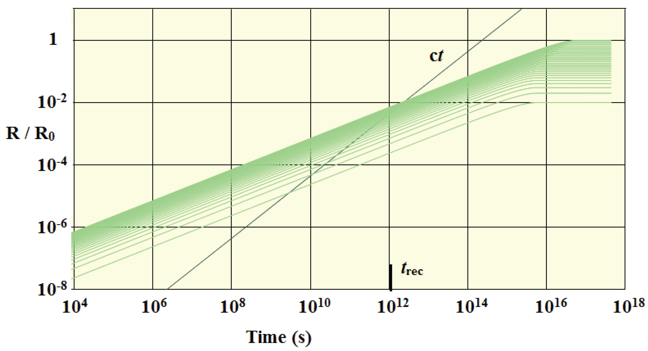
Figure 2.
A 10° square portion of the CMB as seen by the Planck satellite. We see that 1° is characteristic of both the sizes of the superclusters and their spacing.
Figure 2.
A 10° square portion of the CMB as seen by the Planck satellite. We see that 1° is characteristic of both the sizes of the superclusters and their spacing.
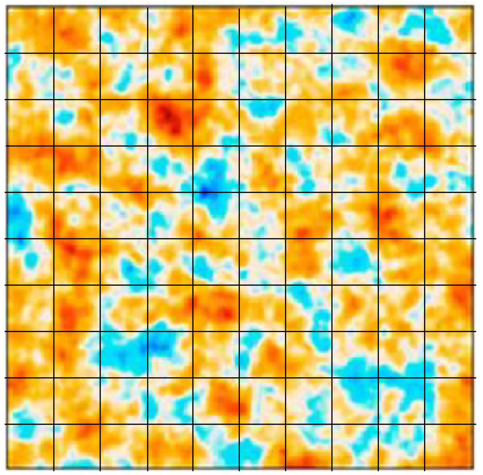
Figure 3.
Example matter distribution. This is a cubic distribution constrained to have zero slope at both the origin and at the outer boundary.
Figure 3.
Example matter distribution. This is a cubic distribution constrained to have zero slope at both the origin and at the outer boundary.
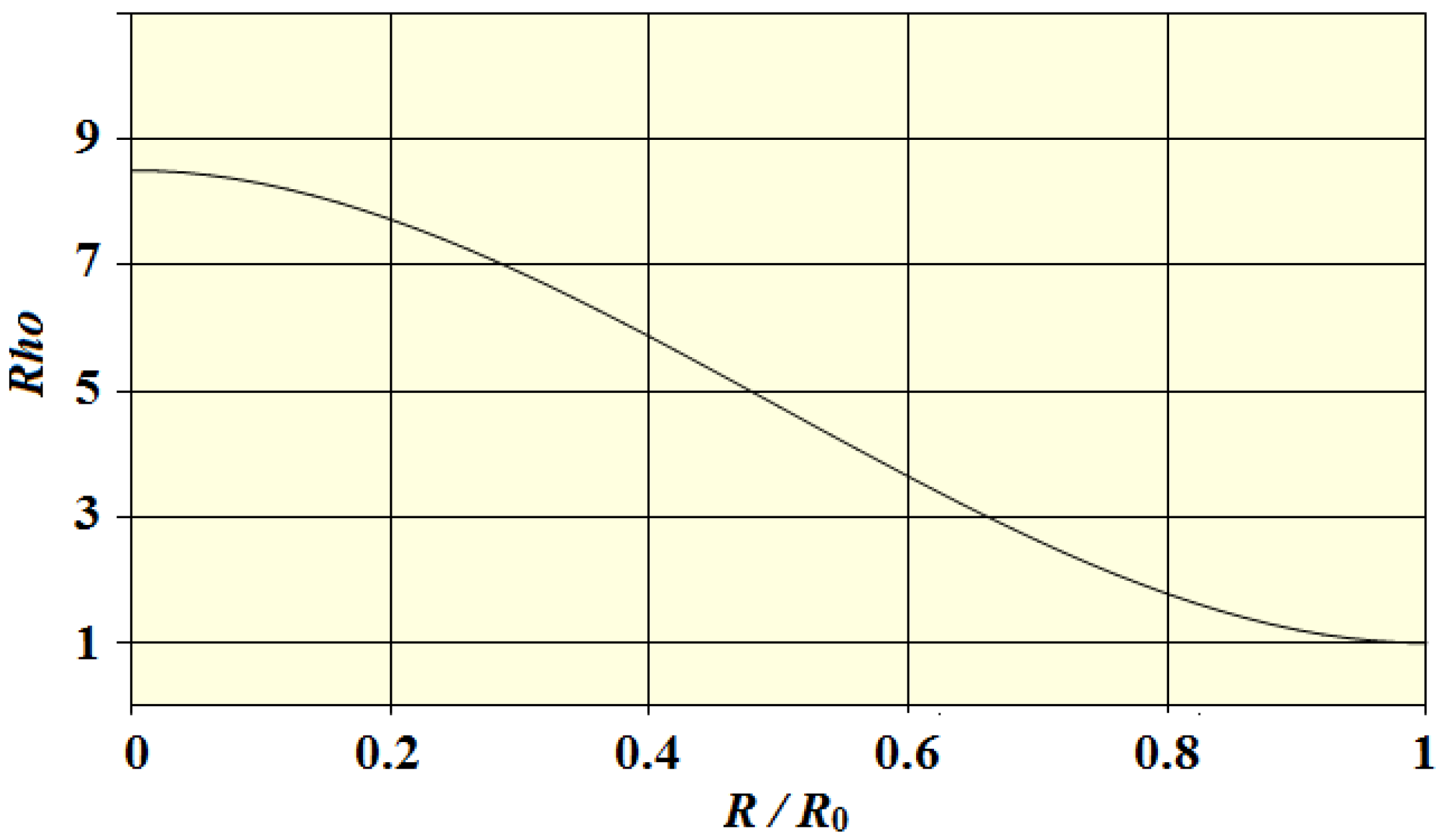
Figure 4.
Recombination free election fraction vs redshift [12].
Figure 4.
Recombination free election fraction vs redshift [12].
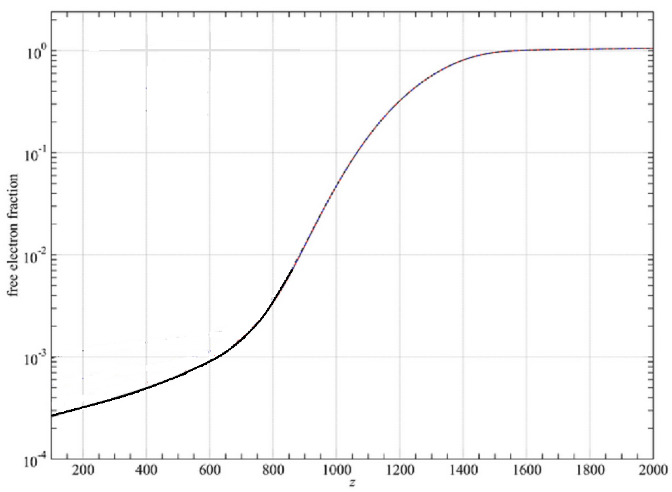
Figure 5.
Last scattering durations vs shell.
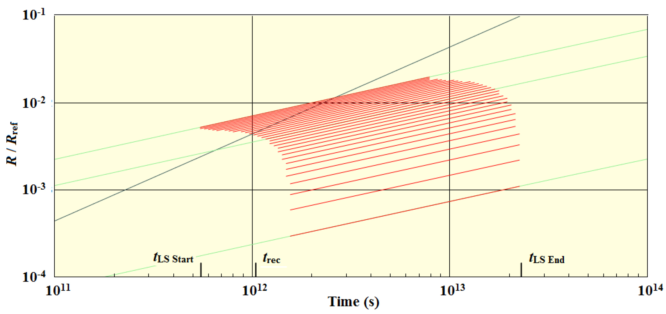
Figure 6.
Mean free paths.
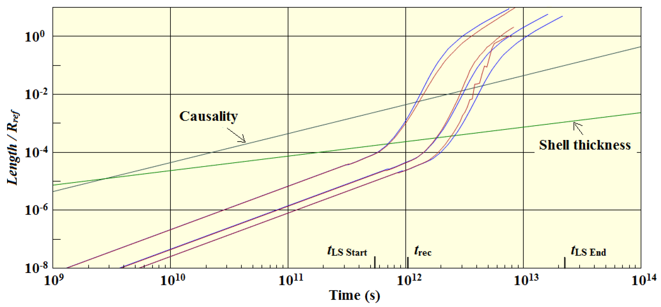
Figure 7.
Intervals per shell during which the scattering per cmb dropped below 1.
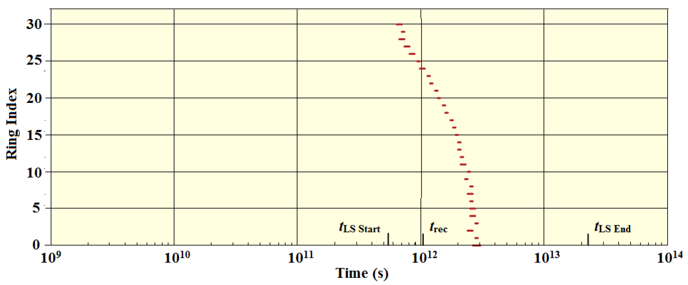
Figure 8.
Total scatters.
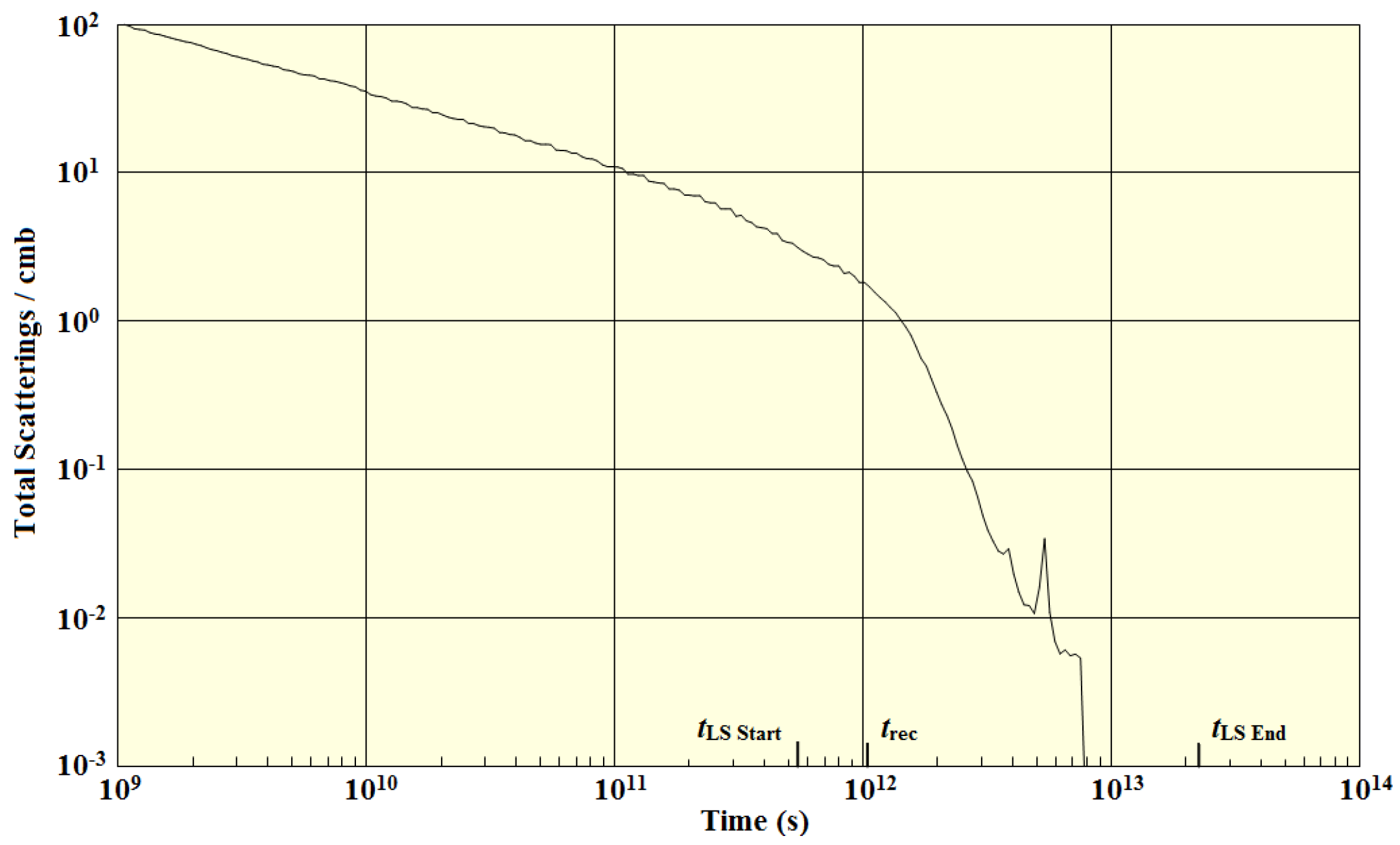
Figure 9.
Number density of cmbs versus distance for a number of simulation times.
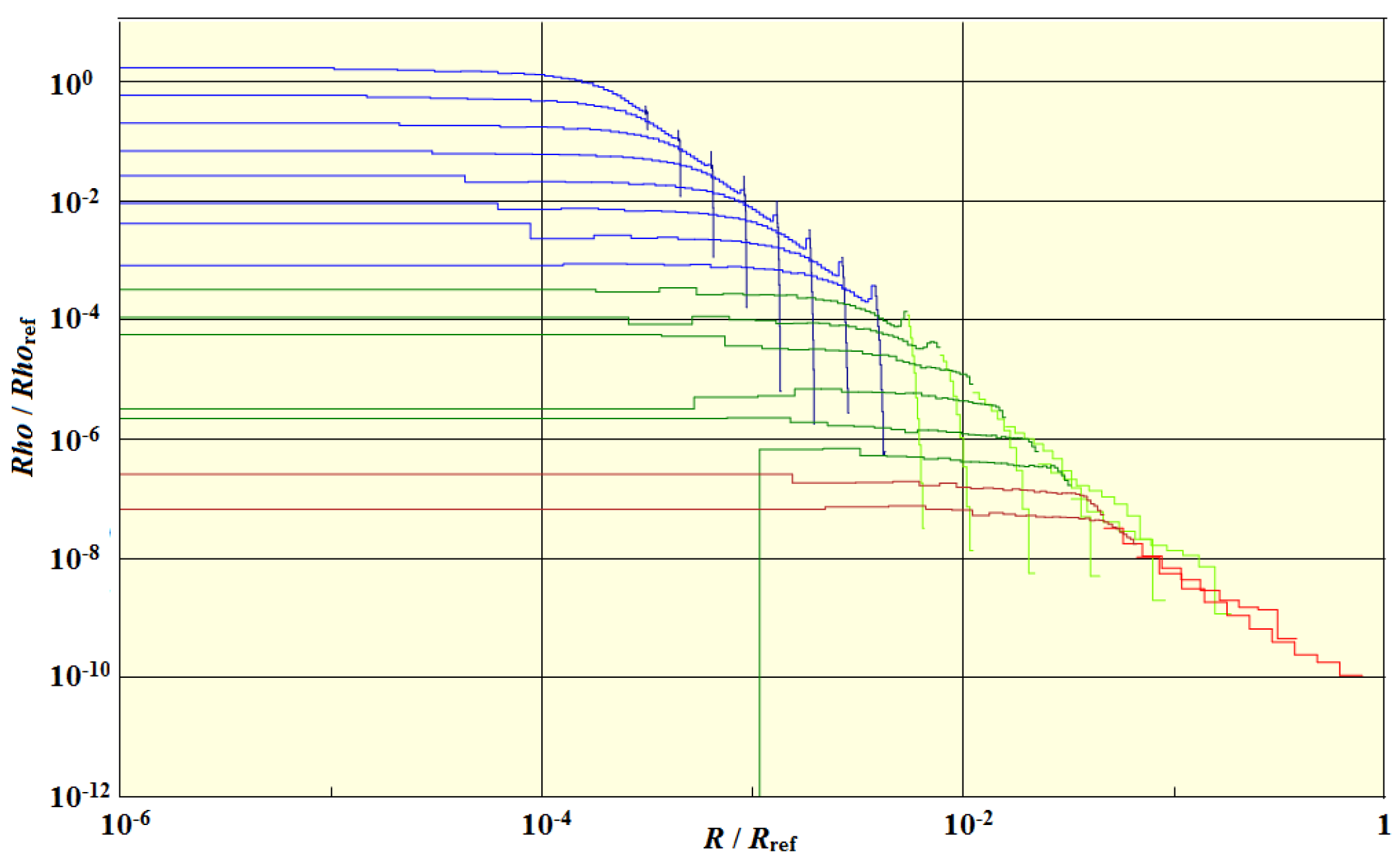
Figure 10.
Temperature versus distance distributions.
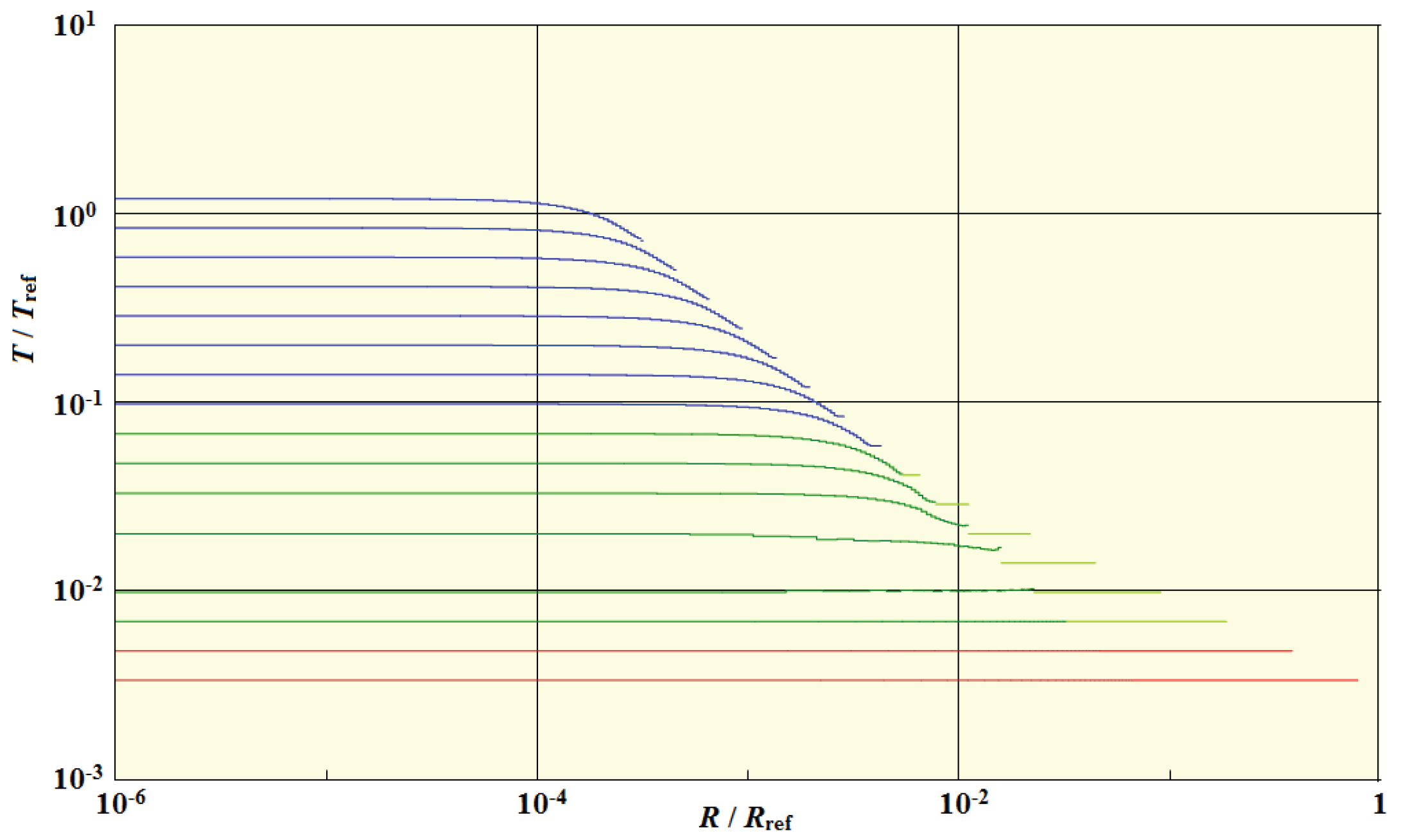
Figure 11.
Count of escaped cmbs with and without scatterings.
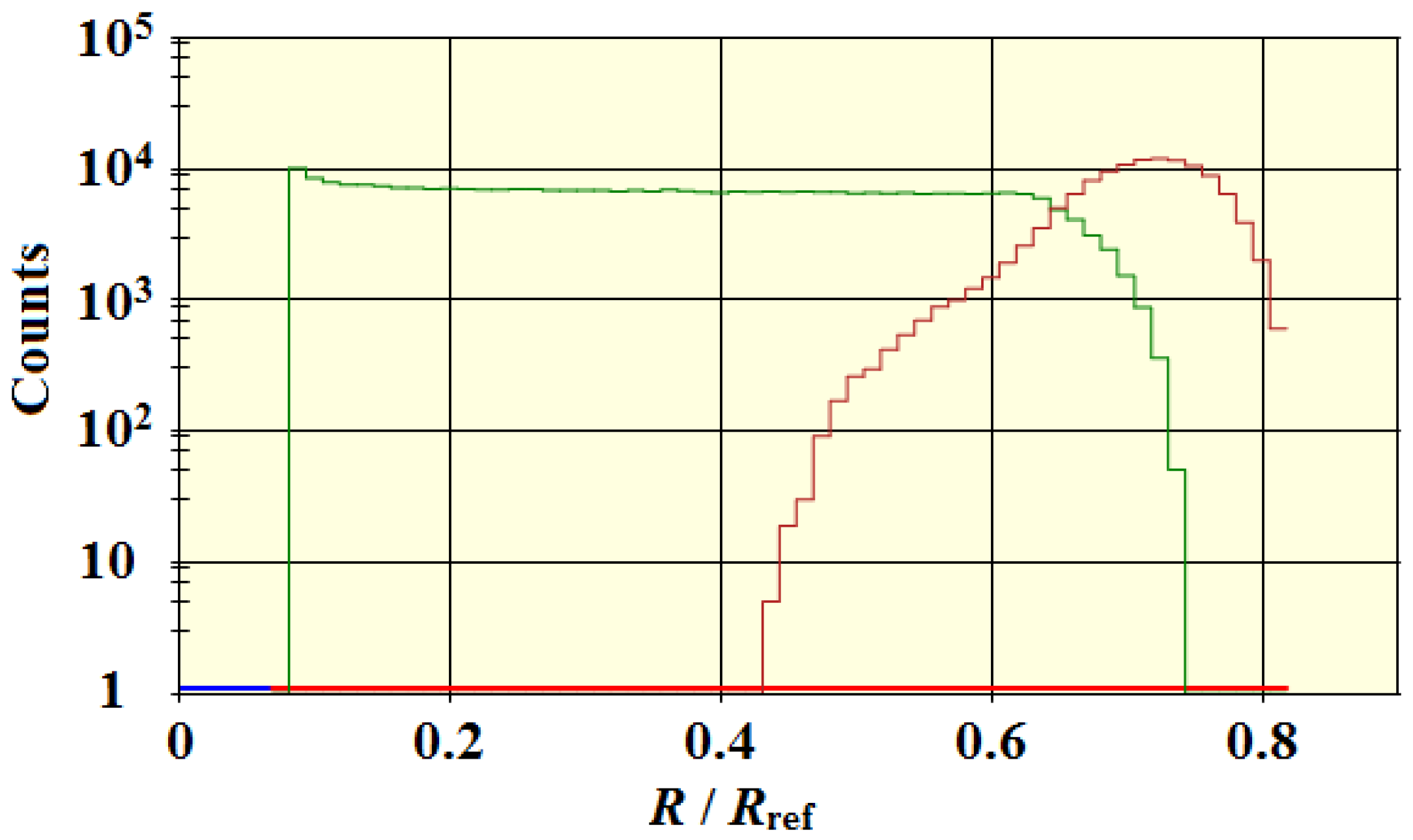
Figure 12.
ratio distribution for the same point in time.
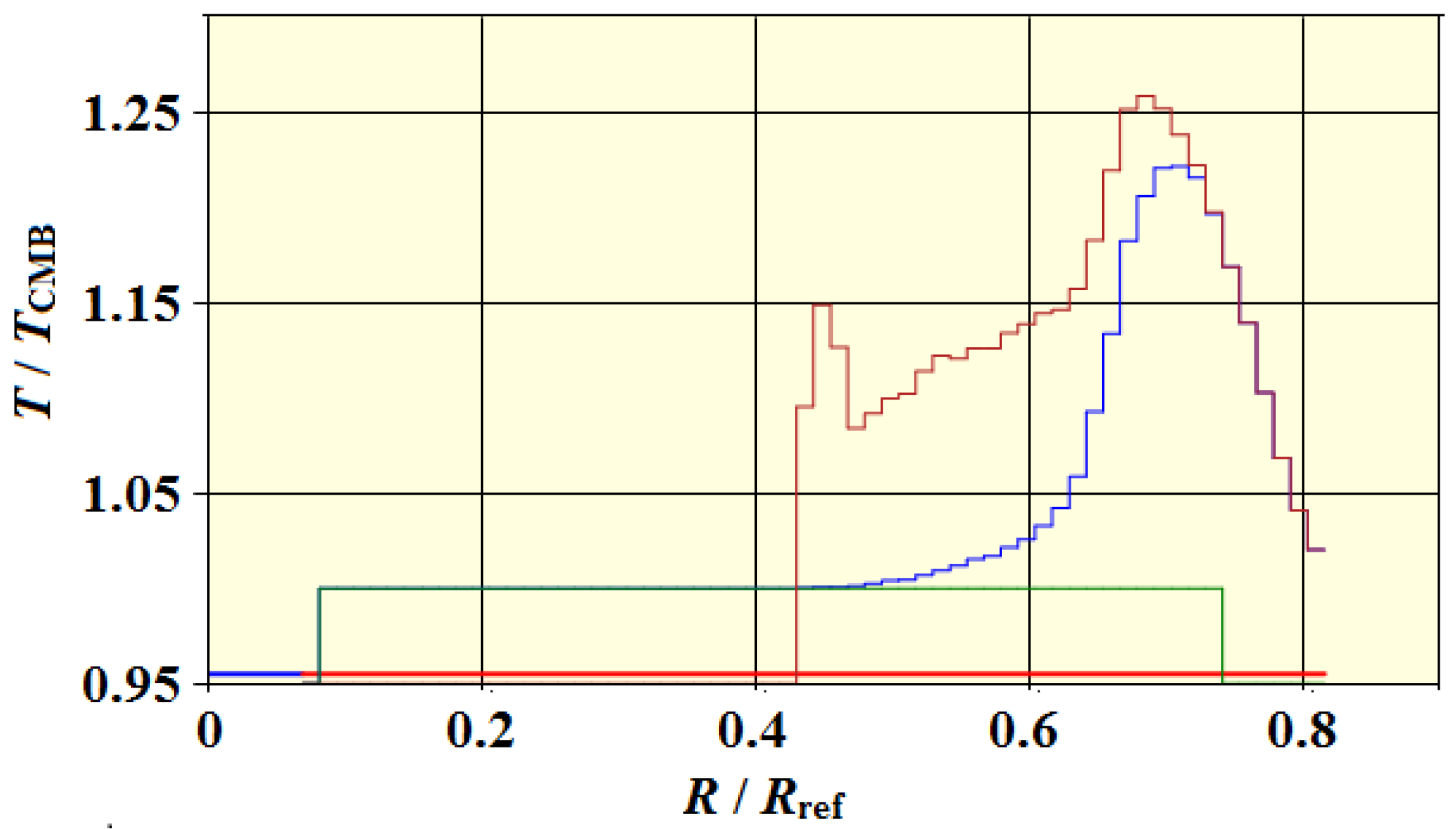
Figure 13.
Peak anisotropy versus time showing the effect of CMB dilution for 3 telescopes.
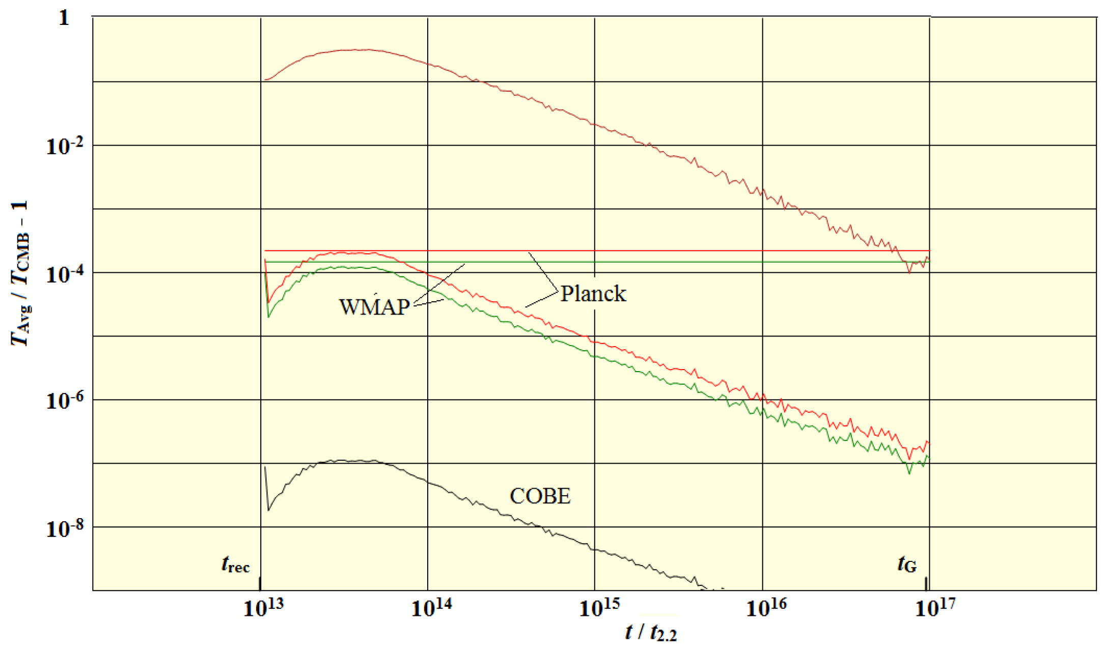
Figure 14.
Scatter plot of the lateral positions of ftons. The left panel shows the ones that underwent at least one scattering, and the right panel shows the ones that had no scatterings.
Figure 14.
Scatter plot of the lateral positions of ftons. The left panel shows the ones that underwent at least one scattering, and the right panel shows the ones that had no scatterings.
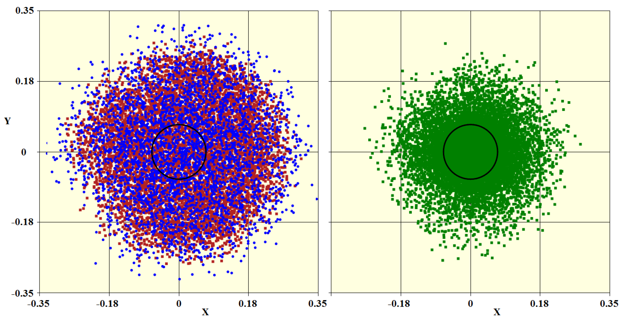
Figure 15.
Scatter plot of ftons with directions within 2 degrees of the z axis. Note the change of scale from the previous figure.
Figure 15.
Scatter plot of ftons with directions within 2 degrees of the z axis. Note the change of scale from the previous figure.
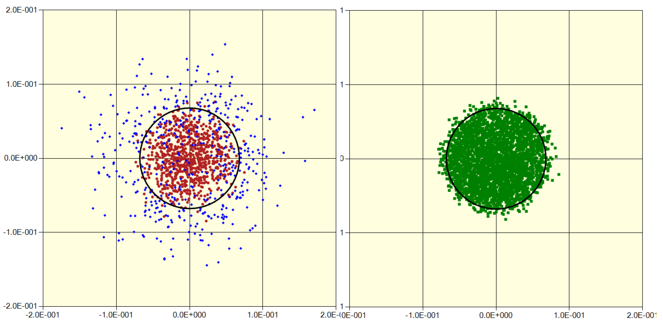
Figure 16.
First detection of CMB polarization which has a 1° scale. The square is 5° on a side.
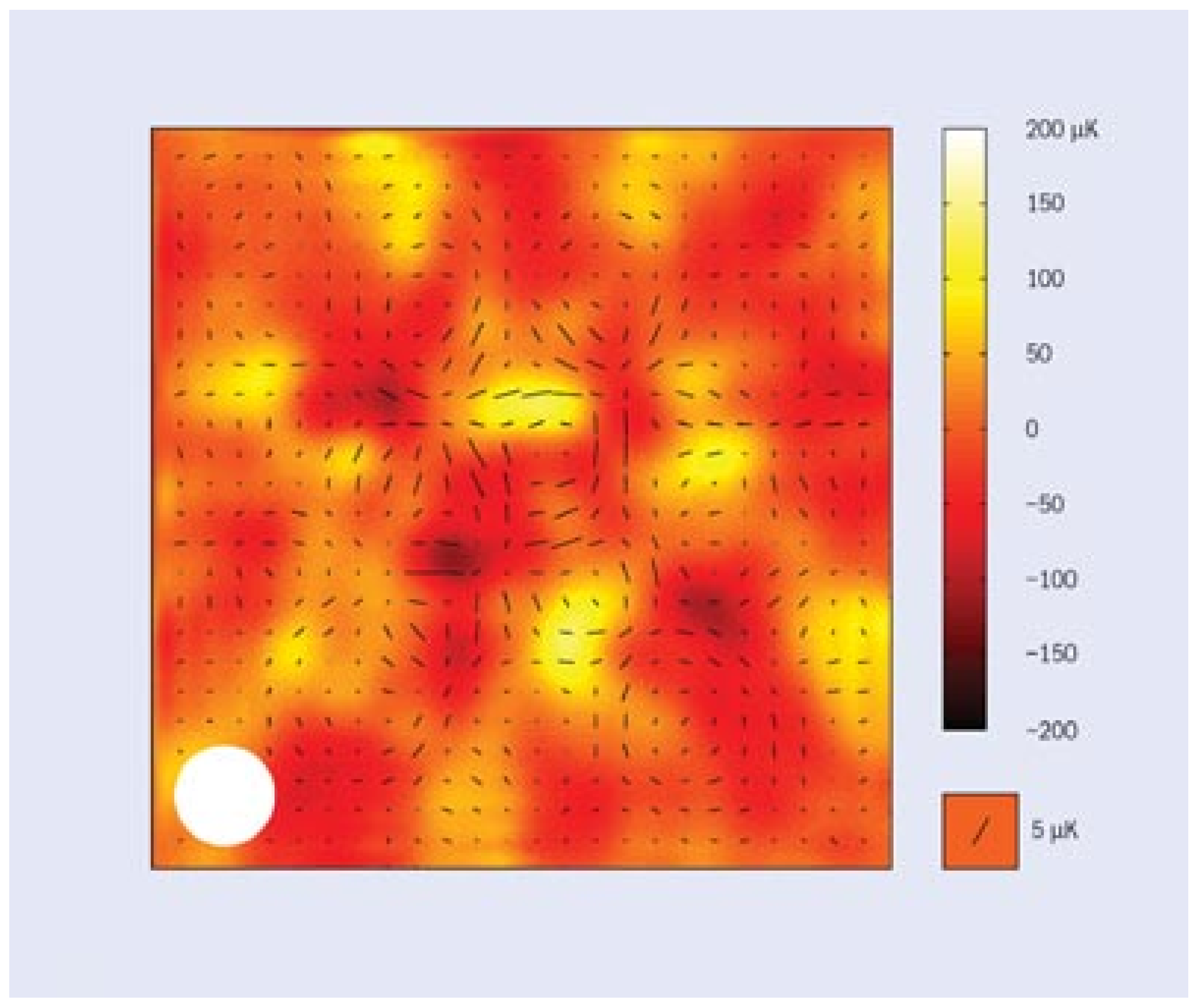
Figure 17.
Measured E-mode polarization with a characteristic scale of 5°. (Adapted from Figure 3 of [17].) The E-mode signal is the Fourier transform of the Stokes parameter distribution of the radiation.
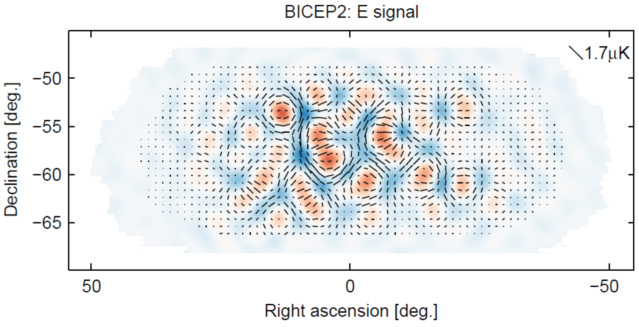
Figure 18.
Distributions of ftons at the specific time of . The green line is the count of ftons that passed through the cluster without scattering, the red line is the count of ftons that last scattered inside the cluster, while the blue line is the count of ftons that last scattered outside the cluster. The parameter z is the distance from the center of the cluster, not the redshift.
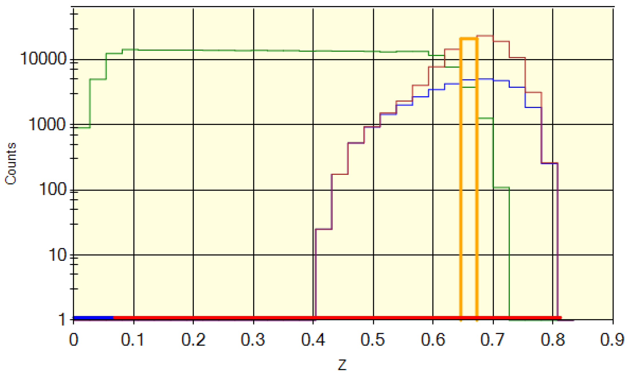
Figure 19.
Polarization from the slice indicated in Figure 16. The radial direction is vertical.
Figure 19.
Polarization from the slice indicated in Figure 16. The radial direction is vertical.
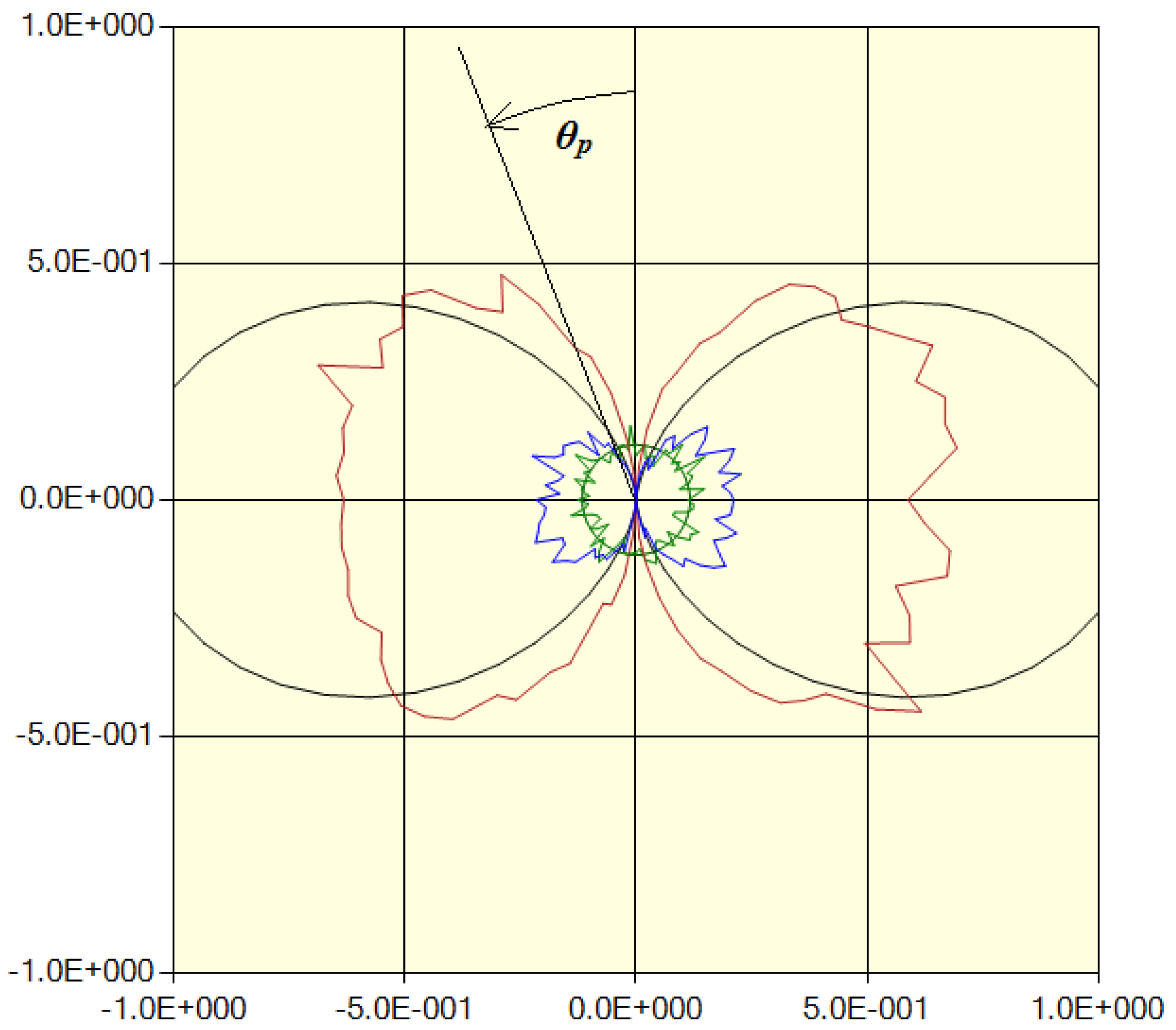
Figure 20.
Same as Figure 19 for a smaller value of z. The green circle is the average of the actual “no scatter” distribution.
Figure 20.
Same as Figure 19 for a smaller value of z. The green circle is the average of the actual “no scatter” distribution.
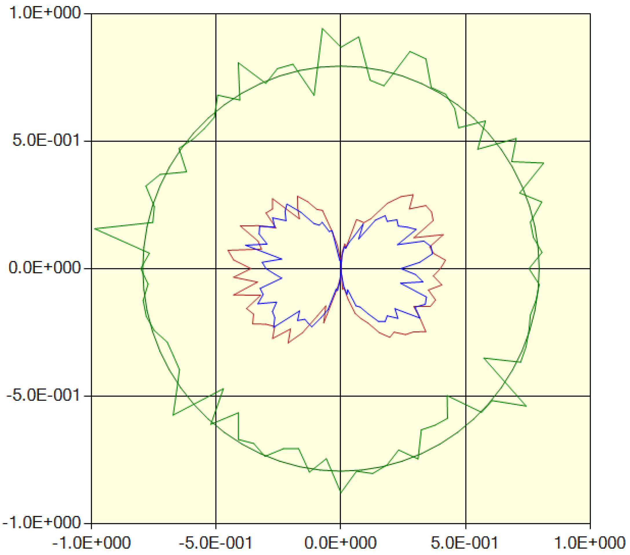
Figure 21.
Polarization for a larger value of z.
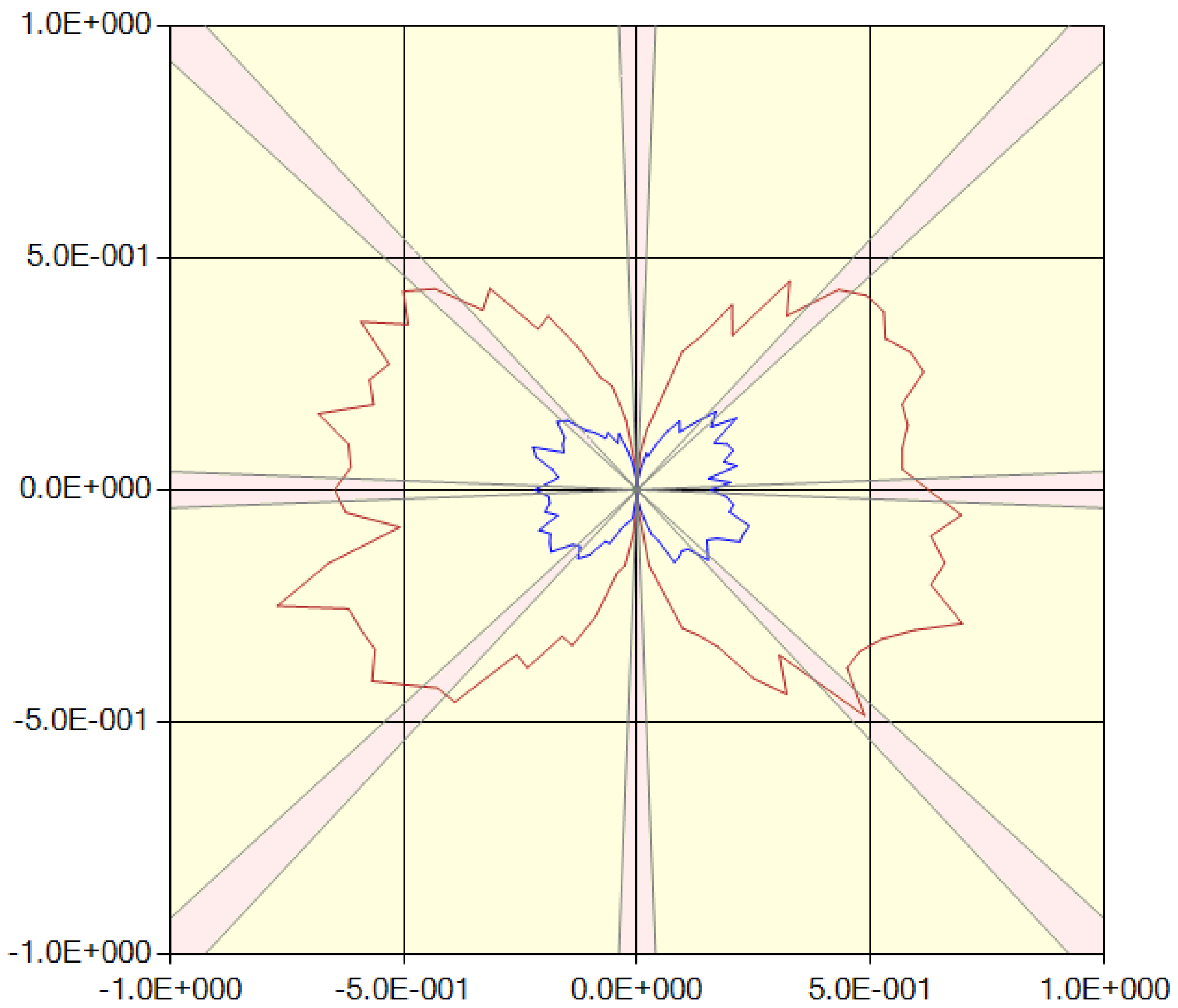
Figure 22.
Degree of polarization as a function of the distance from the center of the cluster.
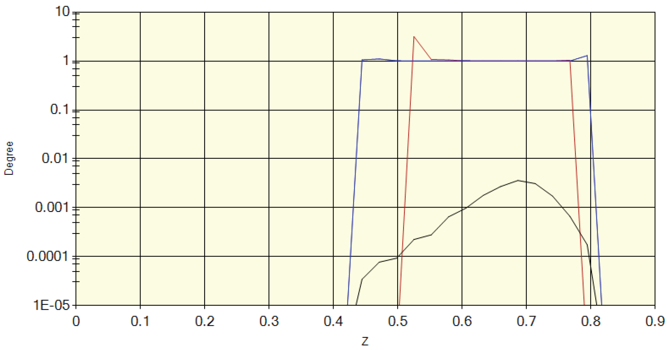

Table 1.
Stokes parameters for the polarization of Figure 21.
Table 1.
Stokes parameters for the polarization of Figure 21.
| Parameter | No Scatter | LS Inside | LS Outside |
|---|---|---|---|
| I | 0.001 | 1.27 | 0.38 |
| Q | 0 | -1.27 | -0.38 |
| U | 0.0054 | 0.0087 | 0.014 |
| Degree | 1.00 | 1.00 |
Disclaimer/Publisher’s Note: The statements, opinions and data contained in all publications are solely those of the individual author(s) and contributor(s) and not of MDPI and/or the editor(s). MDPI and/or the editor(s) disclaim responsibility for any injury to people or property resulting from any ideas, methods, instructions or products referred to in the content. |
© 2026 by the authors. Licensee MDPI, Basel, Switzerland. This article is an open access article distributed under the terms and conditions of the Creative Commons Attribution (CC BY) license (http://creativecommons.org/licenses/by/4.0/).
Copyright: This open access article is published under a Creative Commons CC BY 4.0 license, which permit the free download, distribution, and reuse, provided that the author and preprint are cited in any reuse.


