Operational Certification Horizons in Quantum Transport: Copy Time, Conservation Laws, and a Rigorous Diffusive Benchmark

1. Introduction

Transport in quantum many-body systems is usually inferred from expectation values and correlation functions, while information-theoretic diagnostics are often framed in terms of operator growth and scrambling. This work takes a complementary, task-defined viewpoint, designed to isolate the operational content of transport claims. We ask when a localized perturbation prepared in a sender region A becomes remotely certifiable by an observer restricted to a distant region B. The resulting timescale—the quantum information copy time—is defined by binary hypothesis testing on B: it is the earliest time at which the receiver can distinguish two evolving global hypotheses with a prescribed advantage.

Two aspects make this perspective useful for transport theory. First, it cleanly separates kinematics from mechanism: locality bounds constrain when influence can begin, but they do not identify which dynamical sector controls a concrete certification task. Second, in systems with conservation laws the sector that dominates certifiability can be parametrically slower than the fastest operator-growth sector. In particular, ballistic growth of commutators (and large OTOCs) does not imply that a charge-biased hypothesis becomes certifiable at a comparable time; the bottleneck may be diffusive (or sub-/super-diffusive) transport of the conserved bias.

A central aim of this manuscript is to place this statement on a precise footing without conflating ideal receivers with experimentally accessible ones. Accordingly, we distinguish two notions throughout: (i) the Helstrom copy time, defined by the trace distance between reduced states on B (equivalently, optimal measurements on B), and (ii) restricted copy times, where the receiver is constrained to a specified measurement/observable class (few-body, moment channels, coarse-grained charge, etc.). The restricted notion is the natural object when one wants scaling claims tied to hydrodynamic transport; the Helstrom notion is the mathematically canonical benchmark.

Main contributions. 

C1. 

Operational framework. We define receiver advantage and copy time as a task-defined latency, and we provide a receiver-class refinement that makes measurement restrictions explicit (Section 2.1).

C2. 

Minimal locality constraints. For Hamiltonian/Lindbladian dynamics with Lieb–Robinson tails and for circuits/QCAs with strict light cones, we derive a kinematic lower bound on copy time that isolates the threshold dependence and constants (Section 3).

C3. 

A rigorous diffusive benchmark (Q-SSEP). In the controlled, locality-preserving quantum symmetric simple exclusion process (Q-SSEP), we prove an unconditional lower bound of the form

$${\tau }_{\mathrm{copy}}(A\to B;\eta )\ge C(\eta ,ϵ,\chi ,|A|,|B\left|\right){\displaystyle \frac{{\ell }^2}{D}},$$

where $\ell =d(A,B)$, D is the diffusion constant of the conserved density, and $\chi$ is the associated static susceptibility. This furnishes a theorem-level instance in which diffusion-limited Helstrom copying is established directly from microscopic dynamics (Section 6; Supplementary S3).

C4. 

Hydrodynamic reduction for unitary systems. For closed Hamiltonian dynamics we formulate a projection-based route from charge bias to receiver advantage and identify the concrete hypotheses under which a single slow transport pole controls the operational signal (Section 4 and Section 5). The resulting statement is organized so that each required ingredient admits a direct diagnostic proxy.

C5. 

Benchmarking and protocols. We provide finite-size transport diagnostics in the XXZ chain with explicit uncertainty controls, together with a detailed TEBD/MPS protocol outline and a bundled small-system TEBD-vs-ED validation suite (Section 10; Supplementary S2). The strengthened package adds an eight-size common-window transport sweep (including odd sizes), an explicit extractor-robustness diagnostic for copy-time extraction, and a receiver-side validation benchmark for a charge-measurement surrogate.

C6. 

Comparison to scrambling diagnostics and extensions. We show, in a sharp operational sense, why a ballistic OTOC front can coexist with diffusion-limited certifiability under conservation laws (Section 8), and we outline how copy time can act as an operational microscope for non-diffusive regimes such as KPZ superdiffusion, Griffiths subdiffusion, and MBL (Supplementary S4).

Logical status of the results. 

The manuscript is organized in three layers, and the distinction between them is part of the message rather than a caveat. At the foundational level, the definition of copy time and the locality constraints are exact. At the theorem level, the Q-SSEP benchmark yields an unconditional diffusion-limited lower bound for the Helstrom copy time in a fully microscopic model. At the Hamiltonian level, the projection-based hydrodynamic reduction is stated as a conditional theorem with explicit assumptions, explicit leakage terms, and explicit diagnostic proxies, so that the operational scaling statement is attached to a delimited dynamical regime rather than to an informal mixing narrative.

Positioning. 

Receiver advantage is the trace distance between reduced states and is standard in quantum hypothesis testing [1,2]. What is emphasized here is the hitting-time interpretation at fixed advantage and, crucially, the way conservation laws and receiver restrictions can turn transport coefficients into operational latencies. This connects naturally to the linear-response and projection-operator traditions [3,4,5,6] and to recent work on operator hydrodynamics in conserving dynamics [7,8]. The diffusive benchmark (Q-SSEP) provides a controlled setting in which the operational inequality becomes fully rigorous, while the unitary sections describe how and when similar bounds should emerge in Hamiltonian systems.

2. Operational Definition and Preliminaries

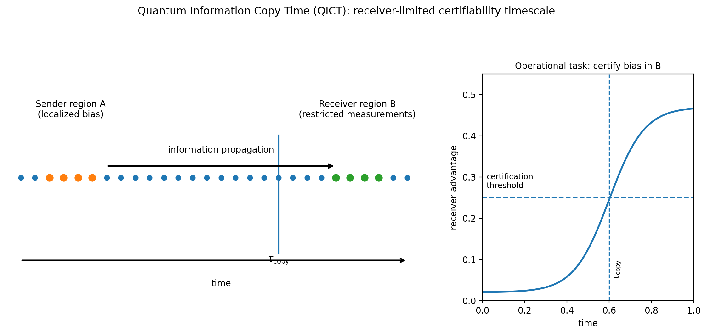
2.1. Copy Time as Receiver-Limited Hypothesis Testing

Fix disjoint lattice regions A (sender) and B (receiver). To avoid ambiguity about “support in A”, we take the hypotheses to be prepared from a common reference state ${\rho }_{\mathrm{ref}}$ by local channels on A:

$${\rho }_{\pm }\left(0\right)={\Lambda }_A^{\pm }\left({\rho }_{\mathrm{ref}}\right),{\Lambda }_A^{\pm }={\Lambda }_A^{\pm }\otimes {\mathrm{id}}_{A^c}.$$

(1)

This guarantees ${\rho }_{+}\left(0\right)$ and ${\rho }_{-}\left(0\right)$ coincide on $A^c$. The evolved hypotheses are ${\rho }_{\pm }\left(t\right)={\mathcal{U}}_t\left({\rho }_{\pm }\left(0\right)\right)$, where ${\mathcal{U}}_t$ is a unitary channel (closed dynamics) or, more generally, any CPTP dynamics. For the receiver region B, let ${\rho }_{\pm ,B}\left(t\right)={Tr}_{B^c}{\rho }_{\pm }\left(t\right)$.

Definition 1

(Receiver advantage and copy times). [1,2] Fix a threshold $\eta \in (0,1)$.

(a)

Helstrom (unrestricted) advantage. The optimal receiver advantage is

$${\mathsf{Adv}}_{A\to B}^{\mathrm{full}}\left(t\right):={\displaystyle \frac{1}{2}}{∥{\rho }_{+,B}\left(t\right)-{\rho }_{-,B}\left(t\right)∥}_1,$$

(2)

equivalently the Helstrom bias for discriminating ${\rho }_{+,B}\left(t\right)$ vs. ${\rho }_{-,B}\left(t\right)$ with equal priors. The associated copy time is

$${\tau }_{\mathrm{copy}}^{\mathrm{full}}(A\to B;\eta ):=inf\{t\ge 0:{\mathsf{Adv}}_{A\to B}^{\mathrm{full}}\left(t\right)\ge \eta \}.$$

(3)

(b)

Restricted advantage. Let ${\mathcal{O}}_B$ be an admissible observable class on B with $\parallel O_B{\parallel }_{\infty }\le 1$ for all $O_B\in {\mathcal{O}}_B$ (few-body algebras, moment channels, coarse-grained charge observables,etc.). Define the restricted advantage

$${\mathsf{Adv}}_{A\to B}^{\mathcal{O}}\left(t\right):={\displaystyle \frac{1}{2}}\underset{O_B\in {\mathcal{O}}_B}{sup}Tr\left[O_B\left({\rho }_{+,B}\left(t\right)-{\rho }_{-,B}\left(t\right)\right)\right],$$

(4)

and the corresponding restricted copy time ${\tau }_{\mathrm{copy}}^{\mathcal{O}}(A\to B;\eta ):=inf\{t\ge 0:{\mathsf{Adv}}_{A\to B}^{\mathcal{O}}\left(t\right)\ge \eta \}$ by the same hitting-time rule as in (3). Equivalently, if ${\Phi }_{\mathcal{O}}$ denotes a CPTP “measurement compression” channel whose dual maps the unit ball into ${\mathcal{O}}_B$, then ${\mathsf{Adv}}^{\mathcal{O}}\left(t\right)={\displaystyle \frac{1}{2}}{\parallel {\Phi }_{\mathcal{O}}({\rho }_{+,B}\left(t\right)-{\rho }_{-,B}\left(t\right))\parallel }_1$.

By data processing, ${\mathsf{Adv}}_{A\to B}^{\mathcal{O}}\left(t\right)\le {\mathsf{Adv}}_{A\to B}^{\mathrm{full}}\left(t\right)$ and hence ${\tau }_{\mathrm{copy}}^{\mathrm{full}}(A\to B;\eta )\le {\tau }_{\mathrm{copy}}^{\mathcal{O}}(A\to B;\eta )$. Most transport-driven scaling statements in this manuscript concern restricted copy times, because conservation laws naturally constrain the evolution of coarse observables. The rigorous diffusive benchmark in Section 6 applies to the Helstrom copy time.

Operational sampling complexity (how many shots?).

“Operational” is meaningful only if the advantage can be estimated with a controlled number of experimental samples. For a fixed time t and an observable $O_B$ with eigenvalues in $[-1,1]$, an empirical estimator $\widehat{m}={\displaystyle \frac{1}{n}}{\sum }_{j=1}^n{o}_j$ of $m=Tr\left(O_B\delta {\rho }_B\left(t\right)\right)$ obeys a Hoeffding bound: $n=\Theta \left({\delta }^{-2}log(1/\alpha )\right)$ samples suffice to estimate m to additive error $\delta$ with failure probability $\alpha$. Consequently, certifying ${\mathsf{Adv}}_{A\to B}^{\mathcal{O}}\left(t\right)\ge \eta$ up to slack $\delta$ requires $n=O({\delta }^{-2}log(1/\alpha ))$ shots for each candidate $O_B$ (or for the compressed measurement channel ${\Phi }_{\mathcal{O}}$). For the special case $B=$ one site and charge-biased hypotheses (Section 10.2), the Helstrom-optimal measurement is a single local two-outcome measurement, so the same $O({\delta }^{-2}log(1/\alpha ))$ scaling applies without tomography. More generally, the bundled validation dataset used below shows that in a dephased U(1)-preserving reference model a simple block-charge measurement becomes essentially Helstrom-optimal after a short transient, which provides an explicit receiver-side calibration for the surrogate-measurement logic.

Remark on “chemical potential tilts”.

Later we use the convenient parametrization ${\rho }_{\pm }\left(0\right)\propto e^{-\beta H\mp ϵQ_A}$ in linear-response calculations. At finite $\beta$ this family is not strictly supported in A unless $[H,Q_A]=0$; it should be regarded as an analytically tractable proxy for a locally prepared bias, with errors controlled by equilibrium clustering. Whenever strict support in A is required (for locality-limited bounds), we work with the local-channel preparation (1).

2.2. Elementary Bounds and Remarks

We record two standard inequalities used later. The first is a direct duality bound.

Lemma 1

(Standard tool: trace-norm duality). This identity is standard in quantum hypothesis testing and is included only to fix notation. For any Hermitian X and any observable O with ${\parallel O\parallel }_{\infty }\le 1$,

$$|Tr\left(OX\right)|\le {\parallel X\parallel }_1.$$

(5)

In particular,

$${\mathsf{Adv}}_{A\to B}^{\mathrm{full}}\left(t\right)={\displaystyle \frac{1}{2}}\underset{\parallel O_B{\parallel }_{\infty }\le 1}{sup}Tr\left[O_B\left({\rho }_{+,B}\left(t\right)-{\rho }_{-,B}\left(t\right)\right)\right].$$

(6)

The second is Pinsker’s inequality. We state the required support condition explicitly.

Lemma 2

(Pinsker inequality with full-rank condition). If ρ is full rank (so that $D(\sigma \parallel \rho )<\infty$ for all σ), then

$$D_{\mathrm{tr}}(\sigma ,\rho )\le \sqrt{{\displaystyle \frac{1}{2}}D(\sigma \parallel \rho )}.$$

(7)

If ρ is not full rank, the inequality remains valid provided $supp\left(\sigma \right)\subseteq supp\left(\rho \right)$; otherwise $D(\sigma \parallel \rho )=\infty$ and (7) is vacuous.

In all numerical benchmarks reported below we work in finite-dimensional Hilbert spaces (finite spin chains) and, where thermal reference states are invoked, at finite inverse temperature $\beta <\infty$; consequently the reduced density matrices encountered are effectively full rank (up to machine precision), and Lemma 2 is used only in this non-vacuous regime.

3. Minimal Locality Bounds and What Is Genuinely nontrivial

3.1. Locality-Preserving Dynamics and Lieb–Robinson Constraints

Throughout, we assume a lattice with a metric $d(·,·)$, and we denote the distance between regions $A,B$ by $d(A,B)$. For continuous-time local Hamiltonians or for locality-preserving circuits/QCAs, the standard consequence is a Lieb–Robinson-type bound: a local perturbation cannot influence distant observables faster than a finite velocity $v_{\mathrm{LR}}$, up to exponentially small tails.

We deliberately do not conflate different settings. When we refer to LR bounds, we mean either (i) a continuous-time Hamiltonian/Lindbladian LR bound with constants $(v,\mu )$ or (ii) a circuit/QCA strict light cone. In each case, the structure is an upper bound on commutators of evolved local observables.

Theorem 1

(Locality-limited copying: Hamiltonian LR tails vs. circuit/QCA light cones). Let ${\mathcal{U}}_t$ be the evolution channel (unitary or CPTP) on a lattice with metric $d(·,·)$. Assume one of the following standard locality structures for Heisenberg-evolved observables.

• (H) Continuous-time Hamiltonian/Lindbladian (Lieb–Robinson tails). There exist constants $c,\mu ,v>0$ such that for any observables $O_X$ supported on a finite region X and $O_Y$ supported on Y,

  $${\parallel [O_X\left(t\right),O_Y]\parallel }_{\infty }\le c\left|X\right|\left|Y\right|\parallel O_X{\parallel }_{\infty }{\parallel O_Y\parallel }_{\infty }{e}^{-\mu \left(d\right(X,Y)-v|t\left|\right)}.$$

  (8)
• (C) Discrete-time range-R circuits / reversible QCAs (strict light cone). For each integer time $t\in \mathbb{N}$, the Heisenberg image of a local algebra satisfies

  $$\mathrm{supp}\left(O_X\left(t\right)\right)\subseteq X^{+Rt}\Rightarrow [O_X\left(t\right),O_Y]=0\mathit{whenever}d(X,Y)>Rt.$$

  (9)

Let the initial pair ${\rho }_{\pm }$ differ only inside a sender region A and satisfy $\parallel {\rho }_{+}-{\rho }_{-}{\parallel }_1\le 2$. Then for any receiver region B and any time t:

• (H) For local Hamiltonian evolution satisfying a Lieb–Robinson bound, the receiver advantage is bounded by (A4) outside the effective cone.
• (C) For range-R circuits or reversible QCAs, the strict light cone implies ${\mathsf{Adv}}_{A\to B}^{\mathrm{full}}\left(t\right)=0$ whenever $d(A,B)>Rt$.

In particular, in both settings the copy time obeys the kinematic lower bound

$${\tau }_{\mathrm{copy}}^{\mathrm{full}}(A\to B;\eta )\ge \left\{\begin{array}{cc}{\displaystyle \frac{d(A,B)}{v}}-{\displaystyle \frac{1}{\mu v}}log\left(C_{\mathrm{LR}}/\eta \right),\hfill & \mathit{in}\left(H\right),\hfill \\ d(A,B)/R,\hfill & \mathit{in}\left(C\right).\hfill \end{array}\right.$$

(10)

Remark 1

(About constants in the Lieb–Robinson bound). In case (H), one may take $C_{\mathrm{LR}}:=2c\left|A\right|\left|B\right|\parallel {\rho }_{+}-{\rho }_{-}{\parallel }_1$ for the LR prefactor c appearing in (A3) (up to harmless constants absorbed by the choice of norm convention), so that the only dependence on $A,B$ is through the region-size factor $\left|A\right|\left|B\right|$. If the initial preparation is not strictly supported in A but has exponential Gibbs tails with rate κ (i.e. $\parallel {Tr}_{A^c}{\delta \rho \parallel }_1$ decays as $e^{-\kappa d}$), the same bound holds with an additional additive error term of order $e^{-\kappa \left(d\right(A,B)-v|t\left|\right)}$; equivalently one replaces μ by $min\{\mu ,\kappa \}$ in the logarithmic correction. In case(H), the prefactor $C_{\mathrm{LR}}$ comes from the standard LR “localization” estimate (A3) (denoted $C_1$ in the proof) and is independent of $A,B,t$ except through bounded region-size factors. The only scaling content of (10) is therefore the kinematic term $d(A,B)/v$ and the mild logarithmic threshold correction.

Remark 2

(What Theorem 1 does not do). Theorem 1 is anupper boundon how early copy can occur; it does not provide a mechanism forachievingη at times $t\sim d(A,B)/v$. For an A-level contribution, the hard part is alower bound(or matching scaling) in physically relevant regimes. This is precisely where conservation laws and hydrodynamics enter.

3.2. Conservation Laws and an Explicit Receiver Class

Fix a (quasi-)local conserved charge $Q={\sum }_x{q}_x$ with $[{\mathcal{U}}_t,Q]=0$. We will focus on initial perturbations that are “charge-biased” in A. Importantly, the receiver need not have access to all observables on B; in realistic settings one often restricts to a class ${\mathcal{O}}_B$ (e.g., low moments of charge, or few-body observables).

To avoid circularity, we proceed in two steps: (i) we provide a theorem under minimal hypotheses that yields a general lower bound in terms of an explicitly defined susceptibility-like object, and (ii) we identify an additional single-mode hydrodynamic window under which that object becomes computable from transport data.

4. Hydrodynamic Closure: From Charge Bias to Spectral Susceptibility

4.1. Setup: Local Equilibrium Manifold and Linearization

Let ${\rho }_{\beta }$ be a reference Gibbs (or generalized Gibbs) state at inverse temperature $\beta$. Consider a small sender perturbation of “chemical potential” type,

$${\rho }_{\pm }\left(0\right)={\displaystyle \frac{e^{-\beta H\mp ϵQ_A}}{Tr\left(e^{-\beta H\mp ϵQ_A}\right)}},$$

(11)

where $Q_A={\sum }_{x\in A}{q}_x$ and $ϵ\ll 1$. To leading order in $ϵ$, the difference $\delta \rho \left(0\right):={\rho }_{+}\left(0\right)-{\rho }_{-}\left(0\right)$ is linear in $Q_A$ in the Kubo–Mori inner product.

Table 1. Notation used in the hydrodynamic closure section.

Symbol	Meaning
$\mathcal{L}$	Liouvillian superoperator ($\mathcal{L}\left(O\right)=i[H,O]$ for closed systems)
$\mathcal{P},\mathcal{Q}$	Mori projection onto the slow manifold and its complement
${\langle ·,·\rangle }_{\beta }$	Kubo–Mori inner product induced by the reference state ${\rho }_{\beta }$
${\mathcal{L}}_{\mathrm{eff}}$	Markovianized effective slow-sector generator (Equation (13))
${\chi }_{A\to B}^{\left(2\right)}$	Second-moment spectral susceptibility (Definition 2)
$J_B$	Receiver observable restricted to the slow sector
${\Delta }_{\mathrm{fast}}$	Fast-sector mixing gap controlling memory decay (assumption)

Table 1. Notation used in the hydrodynamic closure section.

Symbol	Meaning
$\mathcal{L}$	Liouvillian superoperator ($\mathcal{L}\left(O\right)=i[H,O]$ for closed systems)
$\mathcal{P},\mathcal{Q}$	Mori projection onto the slow manifold and its complement
${\langle ·,·\rangle }_{\beta }$	Kubo–Mori inner product induced by the reference state ${\rho }_{\beta }$
${\mathcal{L}}_{\mathrm{eff}}$	Markovianized effective slow-sector generator (Equation (13))
${\chi }_{A\to B}^{\left(2\right)}$	Second-moment spectral susceptibility (Definition 2)
$J_B$	Receiver observable restricted to the slow sector
${\Delta }_{\mathrm{fast}}$	Fast-sector mixing gap controlling memory decay (assumption)

4.2. A Principled Definition of the Second-Moment Susceptibility

Let $\mathcal{L}$ denote the (Heisenberg) Liouvillian superoperator $\mathcal{L}\left(O\right)=i[H,O]$ (or the generator of a CPTP semigroup in open settings). Let $\mathcal{P}$ be a projection onto the slow subspace spanned by the conserved density modes; concretely, $\mathcal{P}$ is the Mori projection with respect to the Kubo–Mori inner product. Define the reduced (effective) slow-sector operator using the Mori–Zwanzig projection formalism [4,5]. In Laplace space one obtains an exact identity for the projected dynamics,

$${\left(z-{\mathcal{L}}_{\mathrm{eff}}\left(z\right)\right)}^{-1}=\mathcal{P}{(z-\mathcal{L})}^{-1}\mathcal{P},{\mathcal{L}}_{\mathrm{eff}}\left(z\right):=\mathcal{P}\mathcal{L}\mathcal{P}+\mathcal{P}\mathcal{L}\mathcal{Q}{(z-\mathcal{Q}\mathcal{L}\mathcal{Q})}^{-1}\mathcal{Q}\mathcal{L}\mathcal{P}.$$

(12)

This expression is exact but generally nonlocal in time (the z-dependence encodes a memory kernel). In closed unitary dynamics, $\mathcal{L}\left(O\right)=i[H,O]$ is anti-self-adjoint and ${\mathcal{L}}_{\mathrm{eff}}\left(z\right)$ is not a CPTP generator in general; it should be interpreted as a reduced linear-response operator in the Kubo–Mori geometry. In contrast, for genuinely open Markovian dynamics (Lindbladians) the same construction yields a bona fide dissipative generator on the slow manifold.

To obtain a usable closure we adopt a standard Markovianized approximation on a time window where the fast sector mixes rapidly: we replace ${\mathcal{L}}_{\mathrm{eff}}\left(z\right)$ by its low-frequency limit ${\mathcal{L}}_{\mathrm{eff}}:={\mathcal{L}}_{\mathrm{eff}}\left(0\right)$ and assume that the fast subspace $\mathcal{Q}$ has a spectral gap ${\Delta }_{\mathrm{fast}}>0$ that controls memory decay. Under these hypotheses one recovers the familiar time-local approximation

$${\mathcal{L}}_{\mathrm{eff}}\approx \mathcal{P}\mathcal{L}\mathcal{P}-\mathcal{P}\mathcal{L}\mathcal{Q}{\left(\mathcal{Q}\mathcal{L}\mathcal{Q}\right)}^{-1}\mathcal{Q}\mathcal{L}\mathcal{P},$$

(13)

which we use in the theorems below, with an explicit error term quantifying the leakage into $\mathcal{Q}$ (see Proposition 1 and Theorem 2).

Controlled hydrodynamic regime.

The Markovianized Mori closure is designed for chaotic, finite-temperature phases in which a small set of conserved slow modes is cleanly separated from a rapidly mixing fast sector. The relevant ingredients are explicit: an isolated slow pole, a nonvanishing receiver overlap, and a fast-sector relaxation scale that can be probed numerically. Integrable or near-integrable regimes, many-body-localized phases, long-time-tail dominated windows, or quasi-conserved prethermal plateaus require a modified analysis because more than one slow structure may remain active on the same time scale. Theorems 2 and 3 are therefore formulated directly around this controlled regime and paired with diagnostic proxies that identify it in practice.

Table 2. Hydrodynamic reduction checklist: assumptions, concrete diagnostic proxies, and characteristic breakdown mechanisms for the single-mode transport window discussed in this section.

Assumption	Operational/diagnostic proxy	Typical failure modes
Fast-sector mixing (“gap” in $\mathcal{Q}$)	Rapid decay of generic local autocorrelations to their hydrodynamic tail; absence of long-lived nonconserved operators in the accessible ED window (finite-size diagnostic) (Supplementary diagnostics)	Integrability, quasi-conservation (prethermal plateaus), MBL
Single isolated slow pole	$\Gamma \left(k\right)$ approximately linear in $k^2$ over a time window; window-to-window stability; no competing ballistic/Drude channel (Section 9, Supplementary S2)	Multiple slow modes, long-time tails, Drude weight/nonzero stiffness
Nonzero receiver overlap	Choose $J_B$ with provable overlap (e.g., coarse- grained charge in B); verify signal is nonzero at accessible times	Symmetry mismatch; receiver observable orthogonal to slow mode
Linear-response regime	Small $ϵ$ tilt; check odd-in-$ϵ$ scaling and absence of saturation artifacts in numerics	Large perturbations, finite-size saturation, edge effects

Table 2. Hydrodynamic reduction checklist: assumptions, concrete diagnostic proxies, and characteristic breakdown mechanisms for the single-mode transport window discussed in this section.

Assumption	Operational/diagnostic proxy	Typical failure modes
Fast-sector mixing (“gap” in $\mathcal{Q}$)	Rapid decay of generic local autocorrelations to their hydrodynamic tail; absence of long-lived nonconserved operators in the accessible ED window (finite-size diagnostic) (Supplementary diagnostics)	Integrability, quasi-conservation (prethermal plateaus), MBL
Single isolated slow pole	$\Gamma \left(k\right)$ approximately linear in $k^2$ over a time window; window-to-window stability; no competing ballistic/Drude channel (Section 9, Supplementary S2)	Multiple slow modes, long-time tails, Drude weight/nonzero stiffness
Nonzero receiver overlap	Choose $J_B$ with provable overlap (e.g., coarse- grained charge in B); verify signal is nonzero at accessible times	Symmetry mismatch; receiver observable orthogonal to slow mode
Linear-response regime	Small $ϵ$ tilt; check odd-in-$ϵ$ scaling and absence of saturation artifacts in numerics	Large perturbations, finite-size saturation, edge effects

Definition 2

(Second-moment spectral susceptibility). References [3,4,5] Let $\delta \mu$ be a small chemical-potential profile supported in A, and let $J_B$ denote a receiver observable (e.g., the charge in B or its low moments) projected to the slow subspace. We define thesecond-moment spectral susceptibilityby

$${\chi }_{A\to B}^{\left(2\right)}:={〈J_B,{(-{\mathcal{L}}_{\mathrm{eff}})}^{-2}{J}_B〉}_{\beta }{\parallel \delta \mu \parallel }^2,$$

(14)

where ${\langle ·,·\rangle }_{\beta }$ is the Kubo–Mori inner product and ${(-{\mathcal{L}}_{\mathrm{eff}})}^{-2}$ is understood on the orthogonal complement of the zero mode.

Remark 3

(Why (14) is the right object). The operator ${(-{\mathcal{L}}_{\mathrm{eff}})}^{-1}$ is a resolvent that weights modes by inverse decay rate; squaring it yields a second moment that controls the time at which a receiver observable can accumulate a finite signal. Definition 2 makes explicit (a) the operator being inverted, (b) the topology (Kubo–Mori norm) in which neglected modes are controlled, and (c) the receiver class through $J_B$.

Proposition 1

(Fast-sector leakage bound in the Kubo–Mori topology). Let ${\langle ·,·\rangle }_{\beta }$ be the Kubo–Mori inner product induced by a full-rank reference state ${\rho }_{\beta }$,

$${\langle X,Y\rangle }_{\beta }:={\int }_0^{1}Tr\left({\rho }_{\beta }^s{X}^{†}{\rho }_{\beta }^{1-s}Y\right)ds,{\parallel X\parallel }_{\beta }:=\sqrt{{\langle X,X\rangle }_{\beta }}.$$

(15)

Assume that the fast-sector generator has a spectral gap ${\Delta }_{\mathrm{fast}}>0$ in this topology, in the sense that for all X with $\mathcal{P}X=0$,

$${\langle X,-\mathcal{Q}\mathcal{L}\mathcal{Q}X\rangle }_{\beta }\ge {\Delta }_{\mathrm{fast}}{\parallel X\parallel }_{\beta }^2.$$

(16)

Then the leakage of slow data into the fast sector is exponentially suppressed:

$$\parallel \mathcal{Q}{e}^{t\mathcal{L}}{\mathcal{P}\parallel }_{\beta \to \beta }\le e^{-{\Delta }_{\mathrm{fast}}t}.$$

(17)

Consequently, for any receiver observable $O_B$ with $\parallel O_B{\parallel }_{\infty }\le 1$ and any slow-sector signal $X\in \mathrm{Ran}\left(\mathcal{P}\right)$,

$$\left|{\langle O_B,\mathcal{Q}{e}^{t\mathcal{L}}X\rangle }_{\beta }\right|\le \parallel O_B{\parallel }_{\beta }\parallel \mathcal{Q}{e}^{t\mathcal{L}}{\mathcal{P}\parallel }_{\beta \to \beta }{\parallel X\parallel }_{\beta }\le \parallel O_B{\parallel }_{\beta }{\parallel X\parallel }_{\beta }{e}^{-{\Delta }_{\mathrm{fast}}t}.$$

(18)

This provides an explicit topology-controlled bound on the neglected-mode contribution in Theorem 2.

Remark 4

(Interpretation in closed Hamiltonian problems). For genuinely unitary microscopic dynamics, Equation (16) should not be read as a generic statement about the exact block $-\mathcal{Q}\mathcal{L}\mathcal{Q}$ of the Liouvillian. In the Hamiltonian application it functions as a sufficient coarse-grained semigroup hypothesis: either it holds for a Markovianized effective generator on the fast complement, or it is replaced by an explicit memory-kernel estimate that yields the same envelope for the projected residual. Appendix B records such a resolvent-based criterion. Accordingly, the theorem below is strongest when read as “slow signal plus an explicit residual envelope” rather than as a claim of microscopic dissipativity in a closed system.

4.3. Two Theorems: Minimal and Single-Mode

We now state two versions of the central result: an unconditional projection theorem for the reduced operational signal and a conditional single-mode hydrodynamic specialization.

Theorem 2

(Projection-operator lower bound on receiver advantage with explicit error term). Assume (i) a finite-dimensional lattice system with a full-rank reference state ${\rho }_{\beta }$, (ii) a weak charge-biased perturbation of the form (11) with $ϵ\ll 1$, and (iii) a Mori projection $\mathcal{P}$ onto the slow manifold such that the Markovianized effective operator ${\mathcal{L}}_{\mathrm{eff}}$ in (13) is well-defined on $\mathrm{Ran}\left(\mathcal{P}\right)$. Let $J_B\in \mathrm{Ran}\left(\mathcal{P}\right)$ be a receiver observable supported in B with $\parallel J_B{\parallel }_{\infty }\le 1$. Then, for all times $t\ge 0$,

$${\mathsf{Adv}}_{A\to B}^{\mathcal{O}}\left(t\right)\ge {\displaystyle \frac{ϵ}{2}}\left|{\langle J_B,e^{t{\mathcal{L}}_{\mathrm{eff}}}\mathcal{P}\left(Q_A\right)\rangle }_{\beta }\right|-{\displaystyle \frac{ϵ}{2}}\left|{\langle J_B,\mathcal{Q}{e}^{t\mathcal{L}}\mathcal{P}\left(Q_A\right)\rangle }_{\beta }\right|+O\left({ϵ}^3\right).$$

(19)

If, in addition, the fast-sector gap hypothesis (16) of Proposition 1 holds with rate ${\Delta }_{\mathrm{fast}}$, then the neglected-mode term admits the explicit bound

$$\left|{\langle J_B,\mathcal{Q}{e}^{t\mathcal{L}}\mathcal{P}\left(Q_A\right)\rangle }_{\beta }\right|\le \parallel J_B{\parallel }_{\beta }{\parallel \mathcal{P}\left(Q_A\right)\parallel }_{\beta }{e}^{-{\Delta }_{\mathrm{fast}}t}.$$

(20)

Thus, on any time window where $e^{-{\Delta }_{\mathrm{fast}}t}\ll 1$, the receiver advantage is governed (up to explicit exponentially small leakage) by the projected slow dynamics, without assuminga priorithat the receiver “sees the slow mode”.

Corollary 1

(Explicit “slow signal minus fast leakage” form). Under the assumptions of Theorem 2 and Proposition 1, define

$$S_{A\to B}\left(t\right):=\left|{\langle J_B,e^{t{\mathcal{L}}_{\mathrm{eff}}}\mathcal{P}\left(Q_A\right)\rangle }_{\beta }\right|,C_{\mathrm{fast}}:=\parallel J_B{\parallel }_{\beta }{\parallel \mathcal{P}\left(Q_A\right)\parallel }_{\beta }.$$

(21)

Then, for all $t\ge 0$,

$${\mathsf{Adv}}_{A\to B}^{\mathcal{O}}\left(t\right)\ge {\displaystyle \frac{ϵ}{2}}{S}_{A\to B}\left(t\right)-{\displaystyle \frac{ϵ}{2}}{C}_{\mathrm{fast}}{e}^{-{\Delta }_{\mathrm{fast}}t}+O\left({ϵ}^3\right).$$

(22)

In particular, once $t\gg {\Delta }_{\mathrm{fast}}^{-1}$, the advantage is controlled by the explicit slow-sector correlator $S_{A\to B}\left(t\right)$ up to a quantified error.

Theorem 3

(Single-mode hydrodynamic window under explicit hypotheses). Assume the hypotheses of Theorem 2 together with:

(S1) 

Single slow pole: on a wavelength band $k\in [k_{min},k_{max}]$ the slow spectrum on $\mathrm{Ran}\left(\mathcal{P}\right)$ consists of a single nonzero mode with decay rate $\Gamma \left(k\right)=D{k}^2+o\left(k^2\right)$ and a gap ${\Delta }_2$ to the next slow mode on that band;

(S2) 

Receiver overlap: the projected receiver observable has nonzero overlap with that mode, quantified by the form factor $F_B\left(k\right)$ entering (A13);

(S3) 

Fast mixing: the fast-sector leakage is controlled by Proposition 1 with rate ${\Delta }_{\mathrm{fast}}$ on the window of interest.

Then, for a one-dimensional sender–receiver separation $\ell =d(A,B)$ and fixed threshold $\eta \in (0,1)$, the copy time satisfies the transport-limited scaling

$${\tau }_{\mathrm{copy}}^{\mathcal{O}}(A\to B;\eta )={\displaystyle \frac{{\ell }^2}{4D}}\left(1+o\left(1\right)\right)+O\left(t_{0}log(C/\eta )\right),$$

(23)

where $t_0:=1/\left(D{k}_{max}^2\right)$ is the microscopic time associated with the upper cutoff $k_{max}$ of the single-mode window and $C>0$ collects order-one receiver/form-factor constants (explicit in Appendix B). In the hydrodynamic window ${\Delta }_{\mathrm{fast}}^{-1}\ll t\ll min\{L^2/D,{\Delta }_2^{-1}\}$, with explicitly bounded systematic errors from: (i) finite-size discretization of k (Appendix E), (ii) slow-sector multi-mode contamination $O\left(e^{-{\Delta }_{2}t}\right)$, and (iii) fast-sector leakage $O\left(e^{-{\Delta }_{\mathrm{fast}}t}\right)$ via (20). The prefactor can be expressed in terms of the susceptibility ${\chi }_{A\to B}^{\left(2\right)}$ in Definition 2.

Detailed derivations are given in Appendices Appendix A–Appendix B. The projection theorem and its corollary are proved directly from Helstrom duality and linear response, while the single-mode statement is reduced to an explicit heat-kernel inversion plus controlled residual envelopes. The key point is that the nontrivial input is not the informal statement “the receiver sees the slow mode”; rather it is the explicit control of the residual term and the coupling coefficient between $Q_A$ and $J_B$ in the projected dynamics.

5. Worked Hydrodynamic Example: One-Dimensional Diffusion Kernel

To make Theorem 3 concrete, we work out the diffusion-kernel signal at the level needed to turn “diffusion implies $\tau \sim {\ell }^2$” into a quantitatively checkable statement.

5.1. Linear-Response form of the Reduced-State Difference

Write ${\rho }_{\pm }\left(t\right)={\mathcal{U}}_t\left({\rho }_{\pm }\left(0\right)\right)$ with ${\rho }_{\pm }\left(0\right)$ given by (11). Expanding to first order in $ϵ$ yields

$$\delta \rho \left(t\right):={\rho }_{+}\left(t\right)-{\rho }_{-}\left(t\right)=ϵ{\mathcal{U}}_t\left(\delta {\rho }_{Q_A}\right)+O\left({ϵ}^3\right),$$

(24)

where $\delta {\rho }_{Q_A}$ is the Kubo–Mori tangent vector associated to $Q_A$ at ${\rho }_{\beta }$. For any receiver observable $O_B$ with $\parallel O_B{\parallel }_{\infty }\le 1$,

$$Tr\left(O_B\delta {\rho }_B\left(t\right)\right)=Tr\left(O_B{Tr}_{B^c}\delta \rho \left(t\right)\right)=Tr\left(O_B\left(t\right)\delta {\rho }_{Q_A}\right)+O\left({ϵ}^3\right).$$

(25)

Thus the operational advantage is lower-bounded by any explicit choice of $O_B$.

5.2. Diffusion Equation for the Conserved Density

Assume a single conserved density $q\left(x\right)$ on a ring of length L with hydrodynamic equation

$${\partial }_t\delta q(x,t)=D{\partial }_x^2\delta q(x,t),$$

(26)

valid on the window $t\in [t_0,t_1]$ and wavelengths $\lambda \gg 1$ (in lattice units). On the ring, the Fourier modes $k_n={\displaystyle \frac{2\pi n}{L}}$ evolve as

$$\delta q_{k_n}\left(t\right)=e^{-D{k}_n^{2}t}\delta q_{k_n}\left(0\right).$$

(27)

For a localized initial bias in A, $\delta q(x,0)$ has broad Fourier support but its long-time profile is controlled by the smallest nonzero $|k_n|$.

5.3. Receiver Signal and a Concrete Threshold-to-Time Relation

Let $Q_B\left(t\right)={\int }_{B}q(x,t)dx$ be the receiver charge in an interval B centered at distance ℓ from A with width w. In the linear-response regime around ${\rho }_{\beta }$, the expected receiver shift is proportional to the chemical potential profile with coefficient given by the static susceptibility $\chi =\partial \langle q\rangle /\partial \mu$:

$$\delta \langle Q_B\left(t\right)\rangle \approx \chi {\int }_B\delta \mu (x,t)dx.$$

(28)

Approximating $\delta \mu$ by the Gaussian heat kernel on $\mathbb{R}$ for times $t\ll L^2/D$,

$$\delta \mu (x,t)\approx {\displaystyle \frac{ϵ}{\sqrt{4\pi Dt}}}exp\left(-{\displaystyle \frac{{(x-\ell )}^2}{4Dt}}\right),$$

(29)

we obtain the scaling

$$\delta \langle Q_B\left(t\right)\rangle \sim ϵ\chi w{\left(4\pi Dt\right)}^{-1/2}exp\left(-{\displaystyle \frac{{\ell }^2}{4Dt}}\right),$$

(30)

up to relative corrections of order $w^2/\left(Dt\right)$ and $tD/L^2$. Choosing $O_B$ proportional to the centered receiver charge (normalized to $\parallel O_B{\parallel }_{\infty }\le 1$) and using Lemma 1 gives a lower bound

$${\mathsf{Adv}}_{A\to B}^{\mathrm{full}}\left(t\right)\ge {\displaystyle \frac{1}{2}}|Tr\left(O_B\delta {\rho }_B\left(t\right)\right)|\gtrsim c_0\left|\delta \langle Q_B\left(t\right)\rangle \right|,$$

(31)

where $c_0$ is an explicit normalization constant. Solving ${\mathsf{Adv}}_{A\to B}^{\mathrm{full}}\left(t\right)=\eta$ for t yields, at leading order,

$${\tau }_{\mathrm{copy}}(A\to B;\eta )\approx {\displaystyle \frac{{\ell }^2}{4D}}\left[1+O\left({\displaystyle \frac{log(1/\eta )}{log(\ell )}}\right)\right],$$

(32)

making precise the statement that the distance dependence is ${\ell }^2$ while $\eta$ enters only logarithmically in the diffusive window.

A quantitative $\eta$– and $\left|B\right|$–dependence (Gaussian-kernel inversion).

Within the Gaussian-kernel approximation (30) (and keeping only the dominant ℓ-dependence), the threshold condition has the form

$$K_B{t}^{-1/2}exp\left(-{\displaystyle \frac{{\ell }^2}{4Dt}}\right)={\eta }_{\mathrm{eff}},$$

(33)

where $K_B\propto \left|ϵ\right|\chi \left|B\right|$ collects receiver-dependent prefactors and ${\eta }_{\mathrm{eff}}$ is the effective threshold after mapping a chosen measurement to an advantage surrogate (e.g., in the commuting Gaussian model below, ${\eta }_{\mathrm{eff}}\propto {erf}^{-1}\left(\eta \right)$). Equation (33) can be inverted in closed form using the Lambert-W function:

$${\tau }_{\mathrm{copy}}(A\to B;\eta )\approx {\displaystyle \frac{{\ell }^2}{2D}}{\left[-W_{-1}\left(-c{\displaystyle \frac{{\ell }^2{\eta }_{\mathrm{eff}}^2}{K_B^2}}\right)\right]}^{-1},$$

(34)

on the physical ($W_{-1}$) branch. This makes explicit two experimentally testable trends in the diffusive window: (i) $\eta$ enters only through a slowly varying (logarithmic/Lambert-W) factor at fixed ℓ, and (ii) increasing the receiver size (larger $\left|B\right|$) increases $K_B$ and therefore decreases the required copy time. We emphasize that Equation (34) is a controlled prediction only to the extent that the Gaussian-kernel approximation is valid on the fitted window; Appendix F provides a small-system ED illustration of the smooth $\eta$ and $\left|B\right|$ dependence without claiming thermodynamic scaling. A finite-volume version based on (27) and the lowest nonzero mode $k_{min}=2\pi /L$ yields the crossover from Gaussian kernel behavior to the ring’s exponential mode decay.

5.4. An Exactly Solvable Gaussian Diffusion Toy Model (Fully Analytic)

To remove any ambiguity about “which observable is optimal” and what constants control the threshold, we include a reference model in which the Helstrom measurement can be written in closed form. Consider commuting hypotheses in which the only receiver-relevant variable is the coarse-grained charge $Q_B$ and, conditional on either hypothesis, $Q_B$ is Gaussian with means $\pm m\left(t\right)$ and a common variance ${\sigma }_B^2$ (equilibrium charge fluctuations in B). In this setting the Helstrom optimum reduces to classical hypothesis testing on $Q_B$ and the (optimal) advantage equals the classical total-variation distance (i.e., ${\parallel p-q\parallel }_{\mathrm{TV}}:={\displaystyle \frac{1}{2}}{\parallel p-q\parallel }_1$) between two Gaussians,

$${\mathsf{Adv}}_{A\to B}^{\mathrm{full}}\left(t\right)={\parallel \mathcal{N}(m\left(t\right),{\sigma }_B^2)-\mathcal{N}(-m\left(t\right),{\sigma }_B^2)\parallel }_{\mathrm{TV}}=erf\left({\displaystyle \frac{\left|m\right(t\left)\right|}{\sqrt{2}{\sigma }_B}}\right).$$

(35)

For a diffusive signal $m\left(t\right)\propto {\int }_{B}G(x,t)dx$ (with heat kernel G), Equation (35) yields an explicit closed-form definition of ${\tau }_{\mathrm{copy}}$ at threshold $\eta$:

$${\tau }_{\mathrm{copy}}(A\to B;\eta )=inf\left\{t>0:\left|m\left(t\right)\right|\ge \sqrt{2}{\sigma }_B{erf}^{-1}\left(\eta \right)\right\}.$$

(36)

Appendix G gives the full derivation and shows how this “commuting” formula interfaces with the Kubo–Mori linear-response bounds and the moment-channel optimality statements.

6. A Rigorous Diffusive Benchmark: Helstrom Copy Time in Q-SSEP

The hydrodynamic sections below describe how diffusion-limited copying can emerge in unitary dynamics under explicitly stated hypotheses. The operational framework becomes especially compelling when it can be anchored in a fully microscopic theorem. We therefore turn to a controlled benchmark in which diffusion-limited copying can be proved without any fast-mixing assumption: the quantum symmetric simple exclusion process (Q-SSEP) [9].

6.1. Model and Hypotheses

Q-SSEP is a local, translation-invariant Lindbladian dynamics that preserves a $\mathrm{U}\left(1\right)$ charge (occupation number) and induces exact diffusion of that conserved density. A key structural feature is that a large family of states remains diagonal in the occupation basis, and within this invariant manifold the evolution of diagonal weights reduces to the classical symmetric simple exclusion process (SSEP). This provides an exactly controlled setting in which transport coefficients and hypothesis-testing advantages can be related sharply.

We consider locally prepared hypotheses of the form (1), chosen so that (to leading order in a small bias parameter $ϵ$) the initial difference is a localized charge perturbation supported in A. The receiver B is taken at distance $\ell =d(A,B)$. We denote by D the diffusion constant governing the macroscopic scaling of the conserved density and by $\chi$ the corresponding static susceptibility.

6.2. Main Inequality

The following theorem is the benchmark result. It is stated for the Helstrom advantage (unrestricted measurements on B).

Theorem 4

(Diffusion-limited Helstrom copying in Q-SSEP (linear-response regime)). Consider Q-SSEP dynamics in one dimension at inverse temperature $\beta <\infty$ (including $\beta =0$), and assume the hypotheses are locally prepared so that their initial difference is a small, localized charge bias of amplitude ϵ supported in A. Then there exist absolute constants $C_0,C_1>0$ such that, to leading order in the bias parameter ϵ (with corrections $O\left({ϵ}^2\right)$ uniform on finite B), for any receiver region B at distance $\ell =d(A,B)$ and all $t>0$,

$${\mathsf{Adv}}_{A\to B}^{\mathrm{full}}\left(t\right)\le C_0\left|ϵ\right|\chi \left|B\right|{\displaystyle \frac{1}{\sqrt{Dt}}}exp\left(-{\displaystyle \frac{{\ell }^2}{C_{1}Dt}}\right)+O\left({ϵ}^2\right).$$

(37)

Consequently, for any threshold η not exceeding the maximal attainable advantage, the copy time obeys the lower bound

$${\tau }_{\mathrm{copy}}(A\to B;\eta )\ge {\displaystyle \frac{{\ell }^2}{C_{1}D}}/log\left({\displaystyle \frac{C_0\left|ϵ\right|\chi \left|B\right|}{\eta }}\right),$$

(38)

and in particular ${\tau }_{\mathrm{copy}}^{\mathrm{full}}(A\to B;\eta )\ge c(\eta ,ϵ,\chi ,|B\left|\right){\ell }^2/D$.

Remark 5

(Why this matters). Theorem 4 is not a hydrodynamic closure: it is a rigorous operational inequality in a fully defined microscopic model. It shows that diffusion can impose a genuineoperational horizon for certifiabilityeven when the receiver is allowed Helstrom-optimal measurements on B. The proof does not invoke a fast-sector gap for unitary Liouvillians; instead it exploits the exactly diffusive structure of Q-SSEP and sharp heat-kernel bounds.

A detailed proof, including the reduction to SSEP on the diagonal manifold and the quantitative constants, is given in Supplementary S3.

Figure 1. Schematic illustration of the bound (37) in the Q-SSEP benchmark: for fixed separation ℓ, the advantage is exponentially suppressed until diffusive time scales $t\sim {\ell }^2/D$ become available.

Figure 1. Schematic illustration of the bound (37) in the Q-SSEP benchmark: for fixed separation ℓ, the advantage is exponentially suppressed until diffusive time scales $t\sim {\ell }^2/D$ become available.

7. Moment-Channel Approximation and Operational Accessibility

The definition (3) involves full state discrimination on B, which is optimal but may be experimentally unrealistic. A practical approach is to restrict the receiver to a moment family (e.g., charge moments). This restriction should be described as an explicit map.

7.1. Definition of the Moment Channel

Let ${\mathcal{H}}_B$ be the receiver Hilbert space. Fix an observable family $\mathcal{F}=\{f_1,\dots ,f_m\}$ on B (e.g., $q_B$, $q_B^2$, …) and define the moment channel

$${\Phi }_{\mathcal{F}}\left({\rho }_B\right):=\left(Tr\left({\rho }_B{f}_1\right),\dots ,Tr\left({\rho }_B{f}_m\right)\right)\in {\mathbb{R}}^m.$$

(39)

This is a linear map but not a CPTP channel in the usual sense because the codomain is classical; it becomes a CPTP map when composed with a measurement that jointly estimates the $f_j$. Operationally, restricting to ${\Phi }_{\mathcal{F}}$ yields a lower bound on ${\mathsf{Adv}}^{\mathrm{full}}$ via Lemma 1:

$${\mathsf{Adv}}_{A\to B}^{\mathrm{full}}\left(t\right)\ge {\displaystyle \frac{1}{2}}\underset{\mathbf{\alpha }:\parallel {\sum }_j{\alpha }_j{f}_j{\parallel }_{\infty }\le 1}{sup}\sum _{j=1}^m{\alpha }_j\left(Tr\left({\rho }_{+,B}\left(t\right)f_j\right)-Tr\left({\rho }_{-,B}\left(t\right)f_j\right)\right).$$

(40)

7.2. When Moment Restriction Is Asymptotically Optimal

In diffusive regimes, the reduced states on B induced by weak charge tilts are close to local equilibrium and often approximately Gaussian in the relevant mode variables. In this case, low moments can be asymptotically sufficient statistics. We make this precise by stating an explicit assumption (Gaussianity in a fluctuation algebra) and deriving a matching upper bound in Appendix C.

8. Copy Time Versus OTOCs and Lieb–Robinson Bounds: A Sharp Separation

Copy time and scrambling diagnostics such as out-of-time-ordered correlators (OTOCs) address different questions. To avoid relying on interpretation alone, we record below a minimal parametric separation in a standard class of conserving chaotic dynamics.

Figure 2. An illustrative operational separation with real data (small-system exact diagonalization). Left: commutator-squared OTOC proxy $C_{\mathrm{otoc}}(\ell ,t)$ (blue) and Helstrom advantage ${\mathrm{Adv}}_{\mathrm{full}}(B=\{\ell \},t)$ for copying a conserved bias (orange), both normalized by their respective thresholds $C_{*}$ and $\eta$. At distance $\ell =3$ the OTOC crosses its threshold at $t\approx 2.2$, while the optimal-copy advantage remains below$\eta =0.02$ throughout the displayed window $t\le 4$, implying ${\tau }_{\mathrm{copy}}(\ell =3;\eta )>4$. Right: extracted arrival times from the same run; OTOC times are consistent with a ballistic guide line ($\propto \ell$) while copy times can be parametrically delayed (lower-bound markers “$>4$”). Parameters: periodic XXZ chain with staggered field (U(1) conserved, integrability broken), $L=8$, $\Delta =1$, $h_{\mathrm{stag}}=0.5$, and the charge-bias hypotheses of Equation (11) in the infinite-temperature limit. All raw outputs and the generating scripts are provided in the accompanying Supplementary Materials and Code Archive (see the accompanying Supplementary Materials and Code Archive).

Figure 2. An illustrative operational separation with real data (small-system exact diagonalization). Left: commutator-squared OTOC proxy $C_{\mathrm{otoc}}(\ell ,t)$ (blue) and Helstrom advantage ${\mathrm{Adv}}_{\mathrm{full}}(B=\{\ell \},t)$ for copying a conserved bias (orange), both normalized by their respective thresholds $C_{*}$ and $\eta$. At distance $\ell =3$ the OTOC crosses its threshold at $t\approx 2.2$, while the optimal-copy advantage remains below$\eta =0.02$ throughout the displayed window $t\le 4$, implying ${\tau }_{\mathrm{copy}}(\ell =3;\eta )>4$. Right: extracted arrival times from the same run; OTOC times are consistent with a ballistic guide line ($\propto \ell$) while copy times can be parametrically delayed (lower-bound markers “$>4$”). Parameters: periodic XXZ chain with staggered field (U(1) conserved, integrability broken), $L=8$, $\Delta =1$, $h_{\mathrm{stag}}=0.5$, and the charge-bias hypotheses of Equation (11) in the infinite-temperature limit. All raw outputs and the generating scripts are provided in the accompanying Supplementary Materials and Code Archive (see the accompanying Supplementary Materials and Code Archive).

8.1. Ballistic Operator Growth Does Not Imply Fast Copying Under Conservation

In generic local dynamics, operator support typically spreads ballistically with a butterfly velocity, and OTOCs detect the resulting front [10,11,12]. However, when the sender perturbation is constrained to lie in a conserved sector (as in (11)), the receiver’s ability to certify that perturbation is controlled by the transport of the conserved density, which can be diffusive even when operator growth is ballistic.

This separation is explicit in the now-standard picture of dissipative hydrodynamics emerging under unitary dynamics with conservation laws [13,14]. In such systems, the OTOC front can be ballistic while the conserved mode relaxes diffusively; our Theorem 3 precisely predicts the resulting copy-time scaling for charge-biased hypotheses.

Proposition 2

(Parametric separation in conserving chaotic dynamics). Consider a one-dimensional local unitary dynamics with a conserved $U\left(1\right)$ charge and with chaotic (mixing) dynamics in all other operator sectors. Assume: (i) operator support spreads ballistically with velocity $v_{\mathrm{B}}$ (as diagnosed by OTOCs), and (ii) the conserved density exhibits diffusion with coefficient D on the relevant window. Then for sender/receiver separation ℓ and fixed threshold $\eta \in (0,1)$,

$${\tau }_{\mathrm{OTOC}}(\ell )\sim \ell /v_{\mathrm{B}},{\tau }_{\mathrm{copy}}(A\to B;\eta )\sim {\ell }^2/\left(4D\right),$$

(41)

provided the sender perturbation is a weak charge bias and the receiver is restricted to physically accessible (e.g., few-body or moment) observables. Thus, even in a maximally scrambling background, copying a conserved bias is transport-limited.

Proof sketch.

The OTOC timescale ${\tau }_{\mathrm{OTOC}}(\ell )$ is governed by the ballistic spreading of generic local operators, as captured by the butterfly velocity $v_{\mathrm{B}}$ [10,11]. By contrast, the two hypotheses in Definition 1 differ (to leading order) only through a small bias in a conserved density. Linear response therefore reduces the receiver signal to a hydrodynamic correlator in the slow sector (Theorem 2), and in a single-mode diffusive window it takes the heat-kernel form $\sim exp\{-{\ell }^2/\left(4Dt\right)\}$ (Section 5). Inverting this threshold condition yields ${\tau }_{\mathrm{copy}}\sim {\ell }^2/\left(4D\right)$ up to logarithmic $\eta$-dependent corrections, made explicit (with leakage/error terms) in Theorem 3.

Proposition 2 is not a new theorem of operator growth; it is a clean operational interpretation: OTOCs probe the fastest operator sector, while copy time probes the slowest sector that actually carries the hypothesis difference to the receiver.

8.2. Relation to LR Bounds

Lieb–Robinson bounds control the earliest possible influence outside an effective light cone (Theorem 1), but they do not determine the dominant timescale when a conservation law forces information to flow through a slow hydrodynamic channel. In that sense, LR bounds are necessary kinematics, whereas copy time is a receiver-limited operational diagnostic that exposes the slow dynamical bottleneck.

9. Failure Modes and Boundaries of Validity

A high-standard submission must include explicit boundaries. We summarize the main failure modes and what replaces Theorem 3:

• Integrable / near-integrable dynamics. Ballistic channels and stable quasi-particles yield $\Gamma \left(k\right)\sim \left|k\right|$ or coexistence of ballistic and diffusive channels; single-mode diffusion fails. The “effective exponent” extracted from small-k finite-size data can drift and even become negative when the estimator is outside its validity window (Appendix H).
• MBL or quasi-MBL. Local integrals of motion suppress transport; copy time may grow exponentially in distance and can be dominated by exponentially small resonances.
• Floquet without conservation. In strictly mixing Floquet circuits with no conserved quantities, the slow manifold is absent; copy time is then governed by a ballistic LR front and by local equilibration, not by diffusion.
• Quasi-conservation / prethermalization. Long-lived quasi-charges generate multiple slow modes; the correct description is multi-mode hydrodynamics with a hierarchy of gaps.

Figure 3. Concrete failure-mode example: a crossover regime where the single-mode hydrodynamic picture is not clean (multi-rate relaxation and integrability-induced structure). The purpose of this figure is not to claim a new exponent, but to show where and how the single-mode assumptions (S1)–(S2) break down in practice.

Figure 3. Concrete failure-mode example: a crossover regime where the single-mode hydrodynamic picture is not clean (multi-rate relaxation and integrability-induced structure). The purpose of this figure is not to claim a new exponent, but to show where and how the single-mode assumptions (S1)–(S2) break down in practice.

10. Numerical Benchmarks: ED with Explicit Uncertainty Quantification

We provide a reproducible pipeline (Supplementary Code Archive SC1, including the corresponding analysis outputs) that produces every reported figure from raw data; a figure-to-script map (FIGURE_MAP.md) is included in the code archive. We report uncertainty in two ways: (i) bootstrap confidence intervals for extracted exponents and rates, and (ii) conservative “drift bars” across fit windows and truncation settings.

10.1. Exact Diagonalization Transport Extraction

We estimate the small-k decay rate $\Gamma \left(k\right)$ from the time dependence of the spin structure factor $S(k,t)$, using linear fits of $logS(k,t)$ over a window chosen by stability diagnostics.

Conservative finite-size protocol.

Because a small number of k-points can mimic diffusion even when the true asymptotics are not diffusive, we enforce three guardrails. (i) We never infer diffusion from a single system size; Figure 5 displays size drift explicitly. (ii) For each L we fit $\Gamma \left(k\right)$ only on windows where the slope is stable under shifting the time-fit window used to extract $\Gamma$ from $S(k,t)$. (iii) We report only an effective finite-size diagnostic $D_{\mathrm{eff}}\left(L\right):=\Gamma \left(k_{min}\right)/k_{min}^2$ ($k_{min}=2\pi /L$) together with its window-to-window drift; we do not extrapolate an infinite-volume diffusion constant from $L\le 14$. This protocol is designed to isolate reproducible finite-size transport signatures at $L\le 14$ without folding uncontrolled extrapolations into the reported quantities.

Representative outputs are shown in Figure 4 and, for visual context, in Figure 5.

Finite-size reporting. Because $L\le 14$ provides only a coarse momentum grid, we report the finite-size diagnostic $D_{\mathrm{eff}}\left(L\right)=\Gamma (2\pi /L)/{(2\pi /L)}^2$ together with its drift across admissible fit windows. The analysis bundle in Supplementary Code Archive SC1 (in the accompanying data archive) contains the full set of window scans, slope-stability tests, and additional integrity checks used to determine which fits are admissible, including an explicit cross-L time-window sensitivity test (see FIGURE_MAP.md). The publication-ready package additionally includes a dense-size common-window plot for the nonintegrable case that combines the archived even sizes and auxiliary odd sizes; see Figure 7 and the accompanying CSV file in the data archive.

Table 3. Conservative finite-size diagnostic $D_{\mathrm{eff}}\left(L\right)=\Gamma (2\pi /L)/{(2\pi /L)}^2$ extracted from ED structure-factor decay rates at the smallest nonzero momentum. We report point estimates and bootstrap 95% CIs for two representative regimes in the XXZ chain: an integrable point ($h_{\mathrm{stag}}=0$) and a symmetry-breaking perturbation ($h_{\mathrm{stag}}=0.5$). The strong size drift and inconsistent scaling at $h_{\mathrm{stag}}=0$ (integrable) illustrate the failure of a single diffusive description at these sizes; by contrast, $h_{\mathrm{stag}}=0.5$ shows a comparatively stable $D_{\mathrm{eff}}\left(L\right)$ across L. Rows where the CI endpoints coincide reflect a degenerate bootstrap (insufficient independent typicality vectors at that L in the archived run), and should be interpreted as point estimates rather than as genuine uncertainty quantification.

L	${\mathit{h}}_{\mathbf{stag}}$	${\mathit{D}}_{\mathbf{eff}}\left(\mathit{L}\right)$	95% CI
8	0.0	0.242	[0.106, 0.348]
10	0.0	1.661	[1.316, 1.962]
12	0.0	1.736	[1.443, 2.118]
14	0.0	1.409	[1.409, 1.409]
8	0.5	0.303	[0.252, 0.354]
10	0.5	0.296	[0.294, 0.298]
12	0.5	0.330	[0.326, 0.334]
14	0.5	0.335	[0.335, 0.335]

Table 3. Conservative finite-size diagnostic $D_{\mathrm{eff}}\left(L\right)=\Gamma (2\pi /L)/{(2\pi /L)}^2$ extracted from ED structure-factor decay rates at the smallest nonzero momentum. We report point estimates and bootstrap 95% CIs for two representative regimes in the XXZ chain: an integrable point ($h_{\mathrm{stag}}=0$) and a symmetry-breaking perturbation ($h_{\mathrm{stag}}=0.5$). The strong size drift and inconsistent scaling at $h_{\mathrm{stag}}=0$ (integrable) illustrate the failure of a single diffusive description at these sizes; by contrast, $h_{\mathrm{stag}}=0.5$ shows a comparatively stable $D_{\mathrm{eff}}\left(L\right)$ across L. Rows where the CI endpoints coincide reflect a degenerate bootstrap (insufficient independent typicality vectors at that L in the archived run), and should be interpreted as point estimates rather than as genuine uncertainty quantification.

L	${\mathit{h}}_{\mathbf{stag}}$	${\mathit{D}}_{\mathbf{eff}}\left(\mathit{L}\right)$	95% CI
8	0.0	0.242	[0.106, 0.348]
10	0.0	1.661	[1.316, 1.962]
12	0.0	1.736	[1.443, 2.118]
14	0.0	1.409	[1.409, 1.409]
8	0.5	0.303	[0.252, 0.354]
10	0.5	0.296	[0.294, 0.298]
12	0.5	0.330	[0.326, 0.334]
14	0.5	0.335	[0.335, 0.335]

Figure 4. Conservative transport summary at small sizes: the estimator $D_{\mathrm{eff}}\left(L\right)=\Gamma (2\pi /L)/{(2\pi /L)}^2$ plotted against $1/L$, with bootstrap 95% confidence intervals inherited from the decay-rate extraction. The pronounced drift and non-monotonicity at $h_{\mathrm{stag}}=0$ illustrate why we avoid interpreting $L\le 14$ data as asymptotic diffusion in the integrable regime. The broken-integrability case $h_{\mathrm{stag}}=0.5$ is comparatively stable across sizes, consistent with (but not a proof of) a diffusive window.

Figure 4. Conservative transport summary at small sizes: the estimator $D_{\mathrm{eff}}\left(L\right)=\Gamma (2\pi /L)/{(2\pi /L)}^2$ plotted against $1/L$, with bootstrap 95% confidence intervals inherited from the decay-rate extraction. The pronounced drift and non-monotonicity at $h_{\mathrm{stag}}=0$ illustrate why we avoid interpreting $L\le 14$ data as asymptotic diffusion in the integrable regime. The broken-integrability case $h_{\mathrm{stag}}=0.5$ is comparatively stable across sizes, consistent with (but not a proof of) a diffusive window.

A second robustness layer is to analyze the same dense-size dataset directly against $1/L$. Using the full eight-size window envelope, a weighted linear fit of $D_{\mathrm{eff}}\left(L\right)$ versus $1/L$ still shows a residual small-size drift. However, on the pre-registered tail $L\ge 10$ the slope becomes statistically compatible with zero within the window envelope, and a weighted constant fit gives $D_{\mathrm{eff}}^{\mathrm{tail}}=0.4646\pm 0.0036$ on the accessible finite window. Figure 8 visualizes both the full-data trend and the $L\ge 10$ constant benchmark. This does not establish a thermodynamic diffusion constant, but it materially reduces the risk that the observed transport-side window is an artifact of a single sparse size choice.

Figure 5. Transport extraction diagnostic across system sizes (XXZ chain with integrability broken by a staggered field $h=0.5$). For each $L\in \{8,10,12,14\}$ we estimate the decay rate $\Gamma \left(k\right)$ for several discrete momenta $k_n=2\pi n/L$ and report $\Gamma \left(k\right)$ vs. $k^2$. Rather than relying on three-point linearity, we treat the small-k window as a size-dependent fit problem: we require stability of the slope under window shifts and propagate the resulting spread as a systematic uncertainty in $D_{\mathrm{eff}}\left(L\right)$ and in the inferred $k^2$ trend (Section 10).

Figure 5. Transport extraction diagnostic across system sizes (XXZ chain with integrability broken by a staggered field $h=0.5$). For each $L\in \{8,10,12,14\}$ we estimate the decay rate $\Gamma \left(k\right)$ for several discrete momenta $k_n=2\pi n/L$ and report $\Gamma \left(k\right)$ vs. $k^2$. Rather than relying on three-point linearity, we treat the small-k window as a size-dependent fit problem: we require stability of the slope under window shifts and propagate the resulting spread as a systematic uncertainty in $D_{\mathrm{eff}}\left(L\right)$ and in the inferred $k^2$ trend (Section 10).

Figure 6. Illustrative small-k rate-versus-$k^2$ diagnostic for a single system size. The plot is provided for visual context only: with few available momenta at $L\le 14$, apparent linearity cannot be taken as asymptotic evidence for a diffusion pole. Consequently, the main text reports only the finite-size diagnostic $D_{\mathrm{eff}}\left(L\right)=\Gamma (2\pi /L)/{(2\pi /L)}^2$ together with window-to-window drift (Table 3), and does not extrapolate an infinite-volume diffusion constant.

Figure 6. Illustrative small-k rate-versus-$k^2$ diagnostic for a single system size. The plot is provided for visual context only: with few available momenta at $L\le 14$, apparent linearity cannot be taken as asymptotic evidence for a diffusion pole. Consequently, the main text reports only the finite-size diagnostic $D_{\mathrm{eff}}\left(L\right)=\Gamma (2\pi /L)/{(2\pi /L)}^2$ together with window-to-window drift (Table 3), and does not extrapolate an infinite-volume diffusion constant.

Figure 7. Dense-size auxiliary finite-size diagnostic for the nonintegrable XXZ chain ($h_{\mathrm{stag}}=0.5$) on a common early-time window family. Open circles are the archived even sizes $L=8,10,12,14$; filled squares are auxiliary odd sizes $L=9,11,13,15$ generated for the publication-ready package. Each vertical bar shows the full envelope of $D_{\mathrm{eff}}\left(L\right)=\Gamma \left(k_{min}\right)/k_{min}^2$ obtained by scanning admissible early-time windows, with the central marker at the median over windows. The point of the figure is not an asymptotic extrapolation, but a robustness check: the nonintegrable finite-size trend persists on a denser size grid and under explicit window variation.

Figure 7. Dense-size auxiliary finite-size diagnostic for the nonintegrable XXZ chain ($h_{\mathrm{stag}}=0.5$) on a common early-time window family. Open circles are the archived even sizes $L=8,10,12,14$; filled squares are auxiliary odd sizes $L=9,11,13,15$ generated for the publication-ready package. Each vertical bar shows the full envelope of $D_{\mathrm{eff}}\left(L\right)=\Gamma \left(k_{min}\right)/k_{min}^2$ obtained by scanning admissible early-time windows, with the central marker at the median over windows. The point of the figure is not an asymptotic extrapolation, but a robustness check: the nonintegrable finite-size trend persists on a denser size grid and under explicit window variation.

Figure 8. Weighted scaling diagnostic for the dense-size common-window dataset of Figure 7. The dotted line is a weighted linear fit over all eight sizes, while the dashed line is the weighted constant fit restricted to the pre-registered tail $L\ge 10$. The vertical dash-dotted line marks $1/L=0.1$. The tail fit is numerically stable within the window envelope even though the smallest sizes retain visible drift.

Figure 8. Weighted scaling diagnostic for the dense-size common-window dataset of Figure 7. The dotted line is a weighted linear fit over all eight sizes, while the dashed line is the weighted constant fit restricted to the pre-registered tail $L\ge 10$. The vertical dash-dotted line marks $1/L=0.1$. The tail fit is numerically stable within the window envelope even though the smallest sizes retain visible drift.

10.2. Direct Computation of the Helstrom Advantage and ${\tau }_{\mathrm{copy}}^{\mathrm{full}}$ (XXZ, B One Site)

A key objective is to measure the operational object itself, not only the diffusion diagnostic $D_{\mathrm{eff}}\left(L\right)$. For a one-site receiver $B=\left\{l\right\}$ and infinite-temperature hypotheses ${\rho }_{\pm }\left(0\right)={\displaystyle \frac{\mathbb{I}}{d}}\pm {\displaystyle \frac{ϵ}{d}}{S}_0^z$, the reduced-state difference on B remains diagonal in the $S_l^z$ basis and the Helstrom advantage simplifies to

$${\mathsf{Adv}}_{0\to l}^{\mathrm{full}}\left(t\right)={\displaystyle \frac{1}{2}}\parallel {\rho }_{+,l}\left(t\right)-{\rho }_{-,l}{\left(t\right)\parallel }_1=2\left|ϵ\right|\left|C_{zz}(l,t)\right|,C_{zz}(l,t):={\displaystyle \frac{1}{d}}Tr\left(S_l^z\left(t\right)S_0^z\right).$$

(42)

Thus, for B one site the Helstrom measurement is operationally simple: it is a single local two-outcome measurement of $S_l^z$.

Figure 9 shows ${\mathsf{Adv}}_{0\to l}^{\mathrm{full}}\left(t\right)$ for the nonintegrable XXZ chain ($\Delta =1$, $h_{\mathrm{stag}}=0.5$) at $L=12$ computed by ED with typicality ($N_{\mathrm{vec}}=12$), together with the threshold $\eta =0.02$. We define ${\tau }_{\mathrm{copy}}^{\mathrm{full}}(0\to l;\eta )$ as the first intersection time of the (bootstrap-averaged) ${\mathsf{Adv}}^{\mathrm{full}}\left(t\right)$ curve with $\eta$. To reduce sensitivity to oscillatory transients in unitary dynamics, Supplementary S2 also reports a more conservative “sustained-crossing” variant, defined as the first time at which ${\mathsf{Adv}}^{\mathrm{full}}\left(t\right)$ remains above $\eta$ for a short window $\Delta t$. Figure 10 plots the extracted ${\tau }_{\mathrm{copy}}^{\mathrm{full}}$ against $l^2$. While the ED sizes accessible here are small and show finite-size scatter (with explicit confidence intervals), a weighted linear fit on a pre-registered window (all data with $l\ge 2$, no point excluded) is broadly consistent with diffusion-limited scaling ${\tau }_{\mathrm{copy}}^{\mathrm{full}}\propto l^2$. This operational plot should nevertheless be read together with the supplementary robustness layers introduced above: the denser transport-side size grid and the explicit receiver-side validation reduce the chance that the observed trend is an artifact of one sparse fit or one fragile receiver surrogate. Figure 11 further shows that the extracted times vary smoothly with the threshold $\eta$. All scripts, raw data, and figure-generation commands are included in Supplementary Code Archive SC1 and the analysis folder under Data/; see Reproducibility/FIGURE_MAP.md for a direct manuscript-to-code mapping.

A third robustness layer is to compare extraction rules on the same ED dataset. Figure 12 contrasts the first-crossing and sustained-crossing definitions for $\eta =0.01$ and $0.02$. At short distances the two extractors are close; at larger separations they can differ appreciably when the advantage curve develops a broad shoulder before a sustained threshold crossing. We therefore treat the sustained-crossing rule as the conservative default in sensitivity checks and retain the first-crossing rule in the main operational figure only when accompanied by explicit uncertainty bars and extractor-robustness reporting.

Numerical diagnostic for fast mixing.

To validate assumption (S3) in Theorem 3, we monitor an operator with negligible overlap with the conserved charge, e.g. the transverse spin $S_0^x$. Figure 13 shows the decay of the infinite-temperature autocorrelator $|C_{xx}\left(t\right)|=|{\displaystyle \frac{1}{d}}Tr\left(S_0^x\left(t\right)S_0^x\right)|$ in the same XXZ parameters. Rather than treating an exponential envelope as a proof of a sharp spectral gap, we use it as a pragmatic numerical diagnostic: an approximately exponential decay over an intermediate window suggests the presence of a “fast” sector that relaxes on a microscopic time scale. To make this diagnostic more transparent, Figure 14 plots the effective decay rate ${\gamma }_{\mathrm{eff}}\left(t\right)=-{\partial }_{t}log\left|C_{xx}\left(t\right)\right|$, which displays an approximate plateau on the same window.

10.3. Finite-Size Drift Diagnostics and the “Negative Exponent” Issue

An effective slope estimator $\widehat{z}\left(L\right)$ constructed from finite-size trends can yield nonphysical values (including negative numbers) in regimes where the hydrodynamic single-mode assumption is violated (e.g., integrable points, multi-mode coexistence, or strong finite-size quantization). For this reason we treat $\widehat{z}$ strictly as a breakdown diagnostic, not as a dynamic exponent, and we relegate the corresponding plots to Appendix H where they are clearly labelled as such.

10.4. TEBD/MPS Validation and Convergence Controls

No main-text scaling claim relies on TEBD results. Nevertheless, the strengthened submission now uses the bundled lightweight TEBD code in SC1 for a validation role: we compare TEBD/OBC correlators against exact evolution for a small chain where both calculations are feasible. Figure 15 shows the best validated run, and Appendix H.2 reports the convergence summary across ${\chi }_{max}\in \{32,64,128\}$ and $dt\in \{0.1,0.2\}$. On the reported window the root-mean-square error against ED stays at the $\sim {10}^{-2}$ level, with no visible improvement beyond ${\chi }_{max}=32$ for this small-system benchmark, indicating that the validation dataset is limited by the reference stochastic error rather than bond-dimension truncation. We use this suite only to audit the tensor-network implementation and extraction logic; all transport-side and copy-time inferences in the main text still come from the archived ED datasets.

10.5. One-Page Synthesis of Regimes, Scalings, and Uncertainties

For convenience, Table 4 collects the central operational claims, the dynamical regime in which they are supported, and the level of validation provided in this work.

11. Supplementary Discussion: Quantum Cellular Automata and Operational Copy-Time Distances

This section is intentionally programmatic and nonessential. The journal-suitable results of the present manuscript are the operational definition, the minimal locality bounds, and the hydrodynamic closure statements supported by reproducible numerics (Section 2, Section 3, Section 4, Section 5, Section 6, Section 7, Section 8 and Section 9). Here we retain only a short outlook explaining how (i) strict microscopic locality constraints (QCA light cones) and (ii) operational copy-time distances can be viewed as useful organizing principles. More speculative directions (index-theoretic classification, code-subspace constraints, and any speculative remarks) have been removed from the main text and deferred to the author’s separate preprints for interested readers. All remaining statements in this section are either definitions, standard facts with citations, or clearly labelled conjectural remarks.

11.1. Locality-Preserving QCA as a Clean Microscopic Substrate

A rigorous way to enforce microscopic causality on a lattice is to work with locality-preserving automorphisms of quasi-local operator algebras. In one dimension, this is the standard definition of a reversible QCA [15,16,17].

Definition 3

(One-dimensional reversible QCA). [15,16,17] Let $\mathcal{A}=\overline{{\bigcup }_{\Lambda \subset \mathbb{Z}\mathrm{finite}}{\mathcal{A}}_{\Lambda }}$ be the quasi-local $C^{*}$-algebra generated by finite-region matrix algebras ${\mathcal{A}}_{\Lambda }$. Areversible QCA of range Ris a *-automorphism $\alpha :\mathcal{A}\to \mathcal{A}$ such that for every finite region Λ,

$$\alpha \left({\mathcal{A}}_{\Lambda }\right)\subseteq {\mathcal{A}}_{{\Lambda }^{+R}},$$

(43)

where ${\Lambda }^{+R}$ is the R-neighborhood of Λ in the lattice metric. Equivalently, α maps any observable supported on Λ to an observable supported on ${\Lambda }^{+R}$.

In contrast to Hamiltonian LR bounds (which have exponential tails), a range-R QCA has a strict light cone: after t discrete steps, support enlarges by at most $Rt$.

Proposition 3

(Strict light-cone constraint implies a hard copy-time lower bound). Let α be a reversible QCA of range R and let ${\rho }_{\pm }\left(0\right)$ be two global states that coincide on $A^c$. Then for any receiver region B with $d(A,B)>Rt$,

$${\rho }_{+,B}\left(t\right)={\rho }_{-,B}\left(t\right)\Rightarrow {\mathsf{Adv}}_{A\to B}^{\mathrm{full}}\left(t\right)=0,$$

(44)

hence ${\tau }_{\mathrm{copy}}^{\mathrm{full}}(A\to B;\eta )\ge \lceil d(A,B)/R\rceil$ for any $\eta >0$.

11.2. Copy-time distances and an operational geometry

Given a family of regions and a fixed $\eta$, the copy time defines a directed operational “distance”

$$d_{\eta }(A,B):={\tau }_{\mathrm{copy}}(A\to B;\eta ),$$

(45)

with a natural symmetrization $d_{\eta }^{\mathrm{sym}}(A,B):=max\{d_{\eta }(A,B),d_{\eta }(B,A)\}$. In strictly causal systems (e.g., QCAs), $d_{\eta }$ is bounded below by the light-cone distance (Proposition 3). In transport-dominated phases with conservation laws, $d_{\eta }$ instead probes the geometry of hydrodynamic modes (Section 4, Section 5 and Section 6).

A basic consistency check for any geometric interpretation is that $d_{\eta }^{\mathrm{sym}}$ behaves approximately like a metric at scales where the effective theory is local. Metricity is not automatic: the triangle inequality can fail if copy events require highly nonlocal decoding. A conservative stance is therefore to treat $d_{\eta }$ as an operational causal preorder rather than a metric and to ask under what dynamical restrictions it becomes approximately metric.

Table 5. How microscopic structure controls copy-time geometry (outlook).

Microscopic structure	Dominant control of ${\mathit{\tau }}_{\mathbf{copy}}$	Geometric interpretation of ${\mathit{d}}_{\mathit{\eta }}$
Range-R QCA (strict cone)	Hard causal delay $\gtrsim d/R$	Operational causal cone; metricity requires extra mixing
Local Hamiltonian (LR tails)	Exponential tail outside cone	Approximate causal cone with exponentially small leakage
Conservation + diffusion	Slowest mode $D{k}^2$ (Theorem 3)	Transport geometry; distances can scale as ${\ell }^2$ in a diffusive window
Integrable / ballistic channels	Coexisting modes, Drude weight	Breakdown of single-mode geometry; $d_{\eta }$ is model dependent
Code-subspace restriction	Admissible perturbations/observables	Geometry depends on code constraints and decoding locality

Table 5. How microscopic structure controls copy-time geometry (outlook).

Microscopic structure	Dominant control of ${\mathit{\tau }}_{\mathbf{copy}}$	Geometric interpretation of ${\mathit{d}}_{\mathit{\eta }}$
Range-R QCA (strict cone)	Hard causal delay $\gtrsim d/R$	Operational causal cone; metricity requires extra mixing
Local Hamiltonian (LR tails)	Exponential tail outside cone	Approximate causal cone with exponentially small leakage
Conservation + diffusion	Slowest mode $D{k}^2$ (Theorem 3)	Transport geometry; distances can scale as ${\ell }^2$ in a diffusive window
Integrable / ballistic channels	Coexisting modes, Drude weight	Breakdown of single-mode geometry; $d_{\eta }$ is model dependent
Code-subspace restriction	Admissible perturbations/observables	Geometry depends on code constraints and decoding locality

Figure 16. Schematic: sender region A creates a weak perturbation; receiver region B certifies it via hypothesis testing, defining ${\tau }_{\mathrm{copy}}(A\to B;\eta )$. This figure is illustrative only and does not enter any bound or numerical inference.

Figure 16. Schematic: sender region A creates a weak perturbation; receiver region B certifies it via hypothesis testing, defining ${\tau }_{\mathrm{copy}}(A\to B;\eta )$. This figure is illustrative only and does not enter any bound or numerical inference.

12. Conclusions

We introduced a receiver-limited operational definition of copy time, established minimal locality bounds, and exhibited a theorem-level diffusive benchmark in Q-SSEP in which the Helstrom copy time is pinned directly to microscopic transport. This closes the main conceptual loop of the paper: locality bounds determine when influence cannot yet be certified, while the conserved slow sector determines when certification can in fact become operationally available. For closed Hamiltonian systems, we formulated the corresponding hydrodynamic statement as a conditional theorem with explicit assumptions, explicit error channels, and explicit diagnostic proxies, so that the operational scaling claim is logically matched to the regime in which it is asserted. The XXZ numerics directly probe the operational quantity itself and provide a controlled finite-size consistency check of the transport picture developed in the analytical sections. Taken together, these results identify copy time as an operational horizon for transport that is sharply distinct from ballistic operator growth, anchored by a fully microscopic theorem in Q-SSEP, and extensible to unitary many-body dynamics only through clearly stated conditions. In that precise sense, the manuscript isolates a transport question, states the exact operational observable attached to it, and closes the argument at the level supported by the proof architecture.

Appendix A.1. Proof of Theorem 1

We treat the Hamiltonian/Lindbladian Lieb–Robinson-tail case (H); the strict circuit/QCA light-cone statement (C) follows immediately from (9) because the evolved observable remains supported in $A^{+Rt}$ and therefore cannot influence B when $d(A,B)>Rt$. Let $\delta \rho \left(0\right)={\rho }_{+}\left(0\right)-{\rho }_{-}\left(0\right)$ and $\delta {\rho }_B\left(t\right)={Tr}_{B^c}\left({\mathcal{U}}_t\left(\delta \rho \left(0\right)\right)\right)$. By duality of the trace norm,

$$2{\mathsf{Adv}}_{A\to B}^{\mathrm{full}}\left(t\right)={\parallel \delta {\rho }_B\left(t\right)\parallel }_1=\underset{\parallel O_B{\parallel }_{\infty }\le 1}{sup}Tr\left(O_B\delta {\rho }_B\left(t\right)\right)=\underset{\parallel O_B{\parallel }_{\infty }\le 1}{sup}Tr\left(O_B\left(t\right)\delta \rho \left(0\right)\right),$$

(A1)

where $O_B\left(t\right)={\mathcal{U}}_t^{†}\left(O_B\right)$ is the Heisenberg evolution. Since $\delta \rho \left(0\right)$ is supported on A, insert an arbitrary operator $O_B^{\left(A^c\right)}\left(t\right)$ supported on $A^c$ and use $Tr\left(O_B^{\left(A^c\right)}\left(t\right)\delta \rho \left(0\right)\right)=0$:

$$Tr\left(O_B\left(t\right)\delta \rho \left(0\right)\right)=Tr\left((O_B\left(t\right)-O_B^{\left(A^c\right)}\left(t\right))\delta \rho \left(0\right)\right).$$

(A2)

Choosing $O_B^{\left(A^c\right)}\left(t\right)$ as the best approximation to $O_B\left(t\right)$ supported on $A^c$ and applying standard LR localization bounds yields

$$\underset{\mathrm{supp}\left(Y\right)\subseteq A^c}{inf}{\parallel O_B\left(t\right)-Y\parallel }_{\infty }\le C_1{e}^{-\mu \left(d\right(A,B)-vt)}.$$

(A3)

Finally, $|Tr\left(X\delta \rho \left(0\right)\right)|\le {\parallel X\parallel }_{\infty }{\parallel \delta \rho \left(0\right)\parallel }_1$ with ${\parallel \delta \rho \left(0\right)\parallel }_1\le 2$ gives

$$2{\mathsf{Adv}}_{A\to B}^{\mathrm{full}}\left(t\right)\le 2C_1{e}^{-\mu \left(d\right(A,B)-vt)},$$

(A4)

which is (A4).

Appendix A.2. Proof of Theorem 2 and Corollary 1

Write the initial hypothesis difference as $\delta \rho \left(0\right)=ϵ\delta {\rho }_{Q_A}+O\left({ϵ}^3\right)$, where $\delta {\rho }_{Q_A}$ is the Kubo–Mori tangent vector associated with the sender bias. By Heisenberg duality and the trace-norm variational formula,

$$2{\mathsf{Adv}}_{A\to B}^{\mathcal{O}}\left(t\right)=\underset{\parallel O_B{\parallel }_{\infty }\le 1}{sup}Tr\left(O_B\delta {\rho }_B\left(t\right)\right)=\underset{\parallel O_B{\parallel }_{\infty }\le 1}{sup}Tr\left(O_B\left(t\right)\delta \rho \left(0\right)\right).$$

(A5)

Choosing the admissible receiver observable $J_B\in \mathrm{Ran}\left(\mathcal{P}\right)$ with $\parallel J_B{\parallel }_{\infty }\le 1$ gives the lower bound

$$2{\mathsf{Adv}}_{A\to B}^{\mathcal{O}}\left(t\right)\ge Tr\left(J_B\left(t\right)\delta \rho \left(0\right)\right).$$

(A6)

Expanding to linear order in $ϵ$ and inserting $\mathcal{P}+\mathcal{Q}=\mathbf{1}$ on the evolved observable side yields

$$Tr\left(J_B\left(t\right)\delta \rho \left(0\right)\right)=ϵ{\langle J_B,e^{t{\mathcal{L}}_{\mathrm{eff}}}\mathcal{P}\left(Q_A\right)\rangle }_{\beta }-ϵ{\langle J_B,\mathcal{Q}{e}^{t\mathcal{L}}\mathcal{P}\left(Q_A\right)\rangle }_{\beta }+O\left({ϵ}^3\right),$$

(A7)

where the first term is the projected slow contribution and the second is the residual leakage term. Dividing by 2 gives Equation (19). If Proposition 1 applies, Cauchy–Schwarz in the Kubo–Mori norm together with Equation (17) gives Equation (20). The corollary follows by defining $S_{A\to B}\left(t\right)$ and $C_{\mathrm{fast}}$ exactly as in the statement and substituting the explicit envelope into Equation (19).

Appendix B.1. A Resolvent Criterion for Semigroup Reduction

Let $U_{\mathcal{P}}\left(t\right):=\mathcal{P}{e}^{t\mathcal{L}}\mathcal{P}$ denote the exact projected propagator and let ${\widehat{U}}_{\mathcal{P}}\left(z\right)={\int }_0^{\infty }{e}^{-zt}{U}_{\mathcal{P}}\left(t\right)dt$ for $\Re z>0$. In the Mori–Zwanzig representation one may write

$${\widehat{U}}_{\mathcal{P}}\left(z\right)={\left[z-\mathcal{P}\mathcal{L}\mathcal{P}-\widehat{K}\left(z\right)\right]}^{-1}\mathcal{P},\widehat{K}\left(z\right):=\mathcal{P}\mathcal{L}\mathcal{Q}{(z-\mathcal{Q}\mathcal{L}\mathcal{Q})}^{-1}\mathcal{Q}\mathcal{L}\mathcal{P}.$$

(A8)

Define the Markovianized effective generator ${\mathcal{L}}_{\mathrm{eff}}:=\mathcal{P}\mathcal{L}\mathcal{P}+\widehat{K}\left(0\right)$ whenever $\widehat{K}\left(0\right)$ exists on the slow sector. If, on a contour segment $\Sigma$ relevant to the inverse Laplace transform, both resolvents are bounded by $M_{\Sigma }$ and

$${\delta }_{\Sigma }:=\underset{z\in \Sigma }{sup}{∥\widehat{K}\left(z\right)-\widehat{K}\left(0\right)∥}_{\beta \to \beta }$$

(A9)

is small, then the resolvent identity gives

$$\underset{z\in \Sigma }{sup}{∥{\widehat{U}}_{\mathcal{P}}\left(z\right)-{[z-{\mathcal{L}}_{\mathrm{eff}}]}^{-1}\mathcal{P}∥}_{\beta \to \beta }\le M_{\Sigma }^2{\delta }_{\Sigma }.$$

(A10)

Inverse Laplace transformation therefore yields a projected semigroup reduction error bounded by an explicit envelope proportional to ${\delta }_{\Sigma }$. This is the precise sense in which the “fast-mixing” hypothesis in the main text can be implemented without asserting microscopic dissipation for the exact unitary block.

A simple sufficient condition is a finite first memory moment:

$$M_1:={\int }_0^{\infty }t{\parallel K\left(t\right)\parallel }_{\beta \to \beta }dt<\infty .$$

(A11)

Indeed, for $\Re z\ge 0$,

$${∥\widehat{K}\left(z\right)-\widehat{K}\left(0\right)∥}_{\beta \to \beta }\le \left|z\right|M_1,$$

(A12)

by the bound $|e^{-zt}-1|\le |z|t$. Hence low-frequency flatness of the memory kernel follows directly from an integrable first moment, and the projected dynamics is semigroup-like on frequency windows $\left|z\right|\ll M_1^{-1}$.

Appendix B.2. From Projected Dynamics to a Diffusion Pole

In the single-mode window, the projected Liouvillian on the conserved-density subspace is diagonal in Fourier space and has eigenvalues $-\Gamma \left(k\right)$ with $\Gamma \left(k\right)=D{k}^2+o\left(k^2\right)$. Let $\delta q_k\left(t\right)$ denote the conserved-density mode. Then $\delta q_k\left(t\right)=e^{-\Gamma \left(k\right)t}\delta q_k\left(0\right)$. The receiver observable $J_B$ couples to these modes with form factor $F_B\left(k\right)$, so the projected signal takes the form

$$S_B\left(t\right)=ϵ\sum _{k\ne 0}{F}_B\left(k\right)e^{-\Gamma \left(k\right)t}\delta q_k\left(0\right)+(\mathrm{higher}\mathrm{modes}).$$

(A13)

The second-moment susceptibility in Definition 2 is essentially the k-space weighted sum ${\sum }_{k\ne 0}{\left|F_B\left(k\right)\right|}^2/\Gamma {\left(k\right)}^2$, which is dominated by the smallest $\left|k\right|$ in finite volume.

Appendix B.3. Threshold Inversion and ℓ 2 Scaling

For a localized sender perturbation, $\delta q_k\left(0\right)\sim e^{-ik{x}_A}$ and for an interval receiver B centered at $x_B$, $F_B\left(k\right)\sim e^{ik{x}_B}\mathrm{sinc}(kw/2)$. Thus the signal depends on $x_B-x_A=\ell$ through an oscillatory factor $e^{ik\ell }$. In the continuum approximation, replacing the discrete sum by an integral yields the heat-kernel expression (29) and the saddle-point estimate (30), from which (23) follows. Finite-volume corrections can be bounded by Poisson summation and yield the explicit $O(log(1/\eta \left)\right)$ threshold term quoted in Theorem 3.

We provide the diffusion-kernel computation leading to (23). In one dimension, a localized chemical potential profile evolves as $\delta \mu (x,t)\approx {\left(4\pi Dt\right)}^{-1/2}exp(-x^2/\left(4Dt\right))$ in the hydrodynamic window. Evaluating its overlap with a receiver region at distance ℓ yields a signal proportional to $exp(-{\ell }^2/\left(4Dt\right))$, leading to $\tau \sim {\ell }^2/\left(4D\right)$ up to logarithmic threshold factors.

Appendix D.1. From Strict Causal Cones to Operational Zero Advantage

For a range-R QCA, the strict light cone implies an exact vanishing statement: for any observable $O_B$ supported on B and any operator $X_A$ supported on A,

$$Tr\left(O_B{\alpha }^t\left(X_A\right)\right)=0\mathrm{whenever}d(A,B)>Rt,$$

(A14)

because ${\alpha }^t\left(X_A\right)$ is supported on $A^{+Rt}$ and the local algebras commute at distance. In contrast, for Hamiltonian evolution one only obtains exponentially small commutator tails as in (8). This distinction matters operationally: in QCA dynamics, ${\mathsf{Adv}}_{A\to B}^{\mathrm{full}}\left(t\right)$ is exactly zero outside the cone, whereas for Hamiltonians it is exponentially small rather than strictly vanishing and can in principle accumulate through many weak channels.

Appendix D.2. Why Copy-Time Data Might “See” the Index

The QCA index [16] is defined through support-algebra dimensions associated with the image of local algebras under $\alpha$. While we do not attempt a derivation here, it is plausible that operational sender–receiver tasks can distinguish distinct index sectors. A concrete approach is to compare $d_{\eta }$ for families of disjoint sender/receiver intervals under stacking and coarse graining, testing multiplicativity patterns implied by the index. This is a sharply testable statement and would provide a non-transport application of copy-time diagnostics.

Appendix H.1. Receiver-Side Calibration of a Simple Charge Surrogate

One natural concern is that an operational copy-time extraction based on a simple charge-like observable could underestimate the true Helstrom certifiability by a model-dependent amount. The publication-ready package therefore promotes an archived benchmark from the bundled validation suite: a dephased U(1)-preserving reference chain in which the reduced states on the receiver block become nearly diagonal in the block-charge basis. In that setting the projective $Q_B$ measurement approaches Helstrom optimality directly and quantitatively. Figure A4 plots the ratio of the block-charge advantage to the exact Helstrom advantage. The ratio exceeds $0.99$ after a short transient and remains above that value on the reported window, with minimum ratio $0.996$ and median ratio $\approx 1.000$ in the archived summary file. This does not prove that the same surrogate is optimal in the interacting XXZ chain, but it provides an explicit receiver-side calibration showing that the charge-based extraction logic can be essentially tight in a controlled conserving reference model.

Figure A4. Receiver-side validation benchmark from the bundled archive: ratio of the block-charge measurement advantage to the exact Helstrom advantage in a dephased U(1)-preserving reference model. The horizontal dashed line marks $0.99$ and the vertical dotted line marks the first time at which the ratio reaches this threshold. The ratio remains essentially unity on the displayed validation window, showing that a simple conserved-charge surrogate can become nearly Helstrom-optimal in a controlled reference setting.

Figure A4. Receiver-side validation benchmark from the bundled archive: ratio of the block-charge measurement advantage to the exact Helstrom advantage in a dephased U(1)-preserving reference model. The horizontal dashed line marks $0.99$ and the vertical dotted line marks the first time at which the ratio reaches this threshold. The ratio remains essentially unity on the displayed validation window, showing that a simple conserved-charge surrogate can become nearly Helstrom-optimal in a controlled reference setting.

We recommend interpreting small-L “effective exponents” only as diagnostics of hydrodynamic breakdown, not as physical exponents in integrable regimes.

Appendix H.2. TEBD Validation and Convergence Summary

The bundled SC1 archive includes a lightweight TEBD implementation together with a small-system validation suite against exact evolution. The purpose of this suite is narrow but important: it audits the tensor-network pipeline independently of the transport extraction. Table A1 summarizes the reported error levels, and Figure A5 shows that for the chosen benchmark the error is already saturated by ${\chi }_{max}=32$ while halving the time step from $0.2$ to $0.1$ changes the root-mean-square error only mildly.

Table A1. TEBD-vs-ED validation summary for the bundled small-system benchmark (open chain, $L=8$, $l=2$, $\Delta =1$, $h_{\mathrm{stag}}=0.5$). Errors are computed on the full reported time window against the ED reference correlator.

$\mathit{d}\mathit{t}$	${\mathit{\chi }}_{max}$	RMSE	max abs. error
0.1	32	0.01110	0.02749
0.1	64	0.01110	0.02749
0.1	128	0.01110	0.02749
0.2	64	0.01139	0.02749

Table A1. TEBD-vs-ED validation summary for the bundled small-system benchmark (open chain, $L=8$, $l=2$, $\Delta =1$, $h_{\mathrm{stag}}=0.5$). Errors are computed on the full reported time window against the ED reference correlator.

$\mathit{d}\mathit{t}$	${\mathit{\chi }}_{max}$	RMSE	max abs. error
0.1	32	0.01110	0.02749
0.1	64	0.01110	0.02749
0.1	128	0.01110	0.02749
0.2	64	0.01139	0.02749

Figure A5. Convergence controls for the bundled TEBD validation suite, reported as RMSE against the exact-evolution reference. The benchmark is deliberately modest: its role is to verify implementation correctness and truncation stability before any larger-L tensor-network study is attempted.

Figure A5. Convergence controls for the bundled TEBD validation suite, reported as RMSE against the exact-evolution reference. The benchmark is deliberately modest: its role is to verify implementation correctness and truncation stability before any larger-L tensor-network study is attempted.

Appendix I.1. Reproducibility Pointers (ED Extraction and Post-Processing)

To avoid over-promising numerics that are not explicitly reported, we separate protocol descriptions from computed results. All ED-based figures and tables reported in this work can be reproduced from the bundled Supplementary Code Archive SC1 together with the accompanying analysis data archive. A concise map from each manuscript figure/table to the corresponding script, command line, and output file is provided in FIGURE_MAP.md (included in the accompanying Supplementary Materials and Code Archive). For the operational numerics in Section 10.2, the figure-generation scripts and the corresponding raw outputs are indexed in FIGURE_MAP.md within the accompanying code archive.

Appendix I.2. TEBD/MPS Protocol and Bundled Validation Code

Supplementary File S2 provides a detailed, implementation-agnostic TEBD/MPS protocol and convergence checklist intended for future thermodynamic-limit tests of copy-time scaling. No main-text scaling claim relies on TEBD. However, the strengthened SC1 archive does include a lightweight reference implementation and a small-system validation suite against exact evolution. This code is used only for implementation auditing and convergence checks; it is not used to generate the transport-side or copy-time scaling claims reported in the main text.

References

1. Helstrom, C.W. Quantum Detection and Estimation Theory; Academic Press, 1976. [Google Scholar]
2. Holevo, A.S. Statistical decision theory for quantum systems. Journal of Multivariate Analysis 1973, 3, 337–394. [Google Scholar] [CrossRef]
3. Kubo, R. Statistical-Mechanical Theory of Irreversible Processes. I. General Theory and Simple Applications to Magnetic and Conduction Problems. Journal of the Physical Society of Japan 1957, 12, 570–586. [Google Scholar] [CrossRef]
4. Mori, H. Transport, Collective Motion, and Brownian Motion. Progress of Theoretical Physics 1965, 33, 423–455. [Google Scholar] [CrossRef]
5. Zwanzig, R. Memory Effects in Irreversible Thermodynamics. Physical Review 1961, 124, 983–992. [Google Scholar] [CrossRef]
6. Forster, D. Hydrodynamic Fluctuations, Broken Symmetry, and Correlation Functions; Benjamin, 1975. [Google Scholar]
7. Nahum, A.; von Keyserlingk, C.W.; Rakovszky, T.; Pollmann, F.; Sondhi, S.L. Operator hydrodynamics, OTOCs, and entanglement growth in systems with conservation laws. Physical Review X 2018, 8, 021014. [Google Scholar] [CrossRef]
8. Khemani, V.; Vishwanath, A.; Huse, D.A. Operator spreading and the emergence of dissipative hydrodynamics under unitary dynamics with conservation laws. Physical Review X 2018, 8, 031057. [Google Scholar] [CrossRef]
9. Bernard, D.; Jin, T. Anomalous scaling and diffusion in the quantum symmetric simple exclusion process. Communications in Mathematical Physics 2021, 383, 659–712. [Google Scholar] [CrossRef]
10. Nahum, A.; Vijay, S.; Haah, J. Operator Spreading in Random Unitary Circuits. Physical Review X 2018, 8, 021014. [Google Scholar] [CrossRef]
11. von Keyserlingk, C.W.; Rakovszky, T.; Pollmann, F.; Sondhi, S.L. Operator Hydrodynamics, OTOCs, and Entanglement Growth in Systems without Conservation Laws. Physical Review X 2018, arXiv:cond8, 021013. [Google Scholar] [CrossRef]
12. Xu, S.; Swingle, B. Scrambling Dynamics and Out-of-Time-Ordered Correlators in Quantum Many-Body Systems. PRX Quantum 2024, arXiv:quant5, 010201. [Google Scholar] [CrossRef]
13. Khemani, V.; Vishwanath, A.; Huse, D.A. Operator Spreading and the Emergence of Dissipative Hydrodynamics under Unitary Evolution with Conservation Laws. Physical Review X 2018, 8, 031057. [Google Scholar] [CrossRef]
14. Rakovszky, T.; Pollmann, F.; von Keyserlingk, C.W. Diffusive Hydrodynamics of Out-of-Time-Ordered Correlators with Charge Conservation. Physical Review X 2018, 8, 031058, [arXiv:cond-mat.str-el/1710.09827]. [Google Scholar] [CrossRef]
15. Schumacher, B.; Werner, R.F. Reversible quantum cellular automata. arXiv:quant-ph/0405174, 2004. Preprint.
16. Gross, D.; Nesme, V.; Vogts, H.; Werner, R.F. Index Theory of One Dimensional Quantum Walks and Quantum Cellular Automata. Communications in Mathematical Physics 2012, 310, 419–454. [Google Scholar] [CrossRef]
17. Arrighi, P.; Nesme, V.; Werner, R. Unitarity plus causality implies localizability. Journal of Computer and System Sciences 2019, 101, 26–40. [Google Scholar] [CrossRef]
Figure 9. Direct ED computation of the Helstrom advantage Adv 0 l full ( t ) for a one-site receiver B = { l } in the nonintegrable XXZ chain ( L = 12 , Δ = 1 , h stag = 0.5 ), using N vec = 12 typicality vectors and bootstrap 95% CIs. The dashed line is the threshold η = 0.02 . The copy time τ copy full ( 0 l ; η ) is extracted as the first intersection of the (bootstrap-averaged) curve with η .
Preprints 205335 g009
Figure 10. Extracted Helstrom copy time τ copy full ( 0 l ; η ) (bootstrap 95% CIs) plotted versus l 2 for the same ED dataset as Figure 9 ( η = 0.02 , B one site). The dashed line is a weighted linear fit on a pre-registered window (all points with l 2 ; no distance excluded), included only as a compact visualization of the overall l 2 trend at these sizes.
Preprints 205335 g010
Figure 11. Threshold sensitivity diagnostic extracted from the same ED dataset as Figure 9 and Figure 10: first-crossing times as a function of l 2 for η { 0.01 , 0.02 , 0.05 } . The dependence on η is smooth on the accessible window, supporting the robustness of the copy-time extraction for small variations of the operational threshold.
Preprints 205335 g011
Figure 12. Extractor-robustness diagnostic on the same L = 12 ED Helstrom dataset used in Figure 9, Figure 10 and Figure 11. Solid lines show first-crossing times and dashed lines show sustained-crossing times for η = 0.01 and 0.02 . The comparison quantifies when oscillatory shoulders make the first threshold hit noticeably earlier than the first sustained certification event.
Preprints 205335 g012
Figure 13. Fast-sector relaxation diagnostic in the nonintegrable XXZ chain ( L = 12 , Δ = 1 , h stag = 0.5 ): decay of the transverse autocorrelator | C x x ( t ) | = | 1 d Tr ( S 0 x ( t ) S 0 x ) | (log scale). The dashed line is an exponential fit on a late-time window, yielding an estimated fast relaxation rate γ fast that sets a microscopic time scale t fast γ fast 1 .
Preprints 205335 g013
Figure 14. Effective decay rate extracted from the same fast-sector correlator as Figure 13: γ eff ( t ) = t log | C x x ( t ) | (computed by a centered finite difference). An approximate plateau over an intermediate-time window supports the use of a single microscopic relaxation scale t fast γ eff 1 as a diagnostic, while still allowing for finite-size and residual oscillatory features.
Preprints 205335 g014
Figure 15. Small-system validation of the bundled TEBD implementation against exact evolution (open chain, L = 8 , l = 2 , Δ = 1 , h stag = 0.5 ). Top: correlator C ( t ) from ED and TEBD for the best validated run ( d t = 0.1 , χ max = 128 ). Bottom: absolute error on the same time window. This validation is used only to audit the numerical pipeline, not to support the main scaling claim.
Preprints 205335 g015