Quantum Information Copy Time (QICT): Operational Definition, Minimal Locality Bounds, Hydrodynamic Susceptibilities, and a Programmatic Outlook

Sacha Mohamed

doi:10.20944/preprints202601.0364.v2

Submitted:

30 January 2026

Posted:

02 February 2026

You are already at the latest version

Abstract

We formulate and benchmark an operational timescale—the quantum information copy time—that quantifies how rapidly a localized bias in an initial many-body state becomes remotely certifiable using measurements restricted to a distant receiver region. The definition is intrinsically information-theoretic: for a fixed distinguishability threshold \eta \in (0,1), the copy time \tau_{\mathrm{copy}}(A \to B; \eta) is the earliest time at which the reduced states on B become distinguishable with advantage at least \eta, quantified by the trace distance and equivalently by the optimal Helstrom measurement. We present (i) a minimal theorem that isolates the genuinely nontrivial ingredients—locality, conservation laws, and an explicit receiver-observable class—and (ii) a controlled hydrodynamic closure in which the copy time is governed by a second-moment spectral susceptibility that ties the receiver advantage to the slowest transport mode. We then provide reproducible exact-diagonalization benchmarks in the XXZ chain that (a) extract finite-size transport diagnostics with conservative uncertainty quantification and (b) delineate failure modes in integrable and near-integrable regimes. TEBD/MPS calculations are included only as qualitative cross-checks (Supplementary File S1) and are not used to support asymptotic scaling claims. Finally, we include a brief, clearly separated outlook on how locality-preserving quantum cellular automata (QCA) and code-subspace constraints might shape operational copy-time distances; this material is explicitly conjectural and is not used in any theorem, bound, or numerical claim.

Keywords:

quantum information

;

state discrimination

;

trace distance

;

hydrodynamics

;

quantum cellular automata

;

Lieb–Robinson bounds

;

diffusion

;

operational timescales

Subject:

Physical Sciences - Theoretical Physics

Introduction

The purpose of this paper is twofold. First, we define and analyze a concrete, operational timescale for information propagation in many-body quantum dynamics: the quantum information copy time (QICT). Second, we use this operational object as a micro-level input to a broader, programmatic research direction that aims to connect microscopic locality-preserving unitary dynamics to macroscopic transport, and ultimately to effective causal structure.

The copy time is designed to avoid two common ambiguities. (i) It is not a proxy for “scrambling” in the OTOC sense; rather it measures remote certifiability by a receiver restricted to a spatial region

B

and an admissible measurement class. (ii) It is not tied to a particular coarse-graining scheme: the definition is strictly in terms of quantum hypothesis testing (Helstrom–Holevo theory) on reduced density operators.

To make the scope and logical dependencies explicit, we separate the paper into three layers:

Operational layer (fully general). Definitions and inequalities that hold for arbitrary finite-dimensional quantum systems and any unitary (or CPTP) dynamics.
Hydrodynamic closure layer (assumptions explicit). A theorem that relates copy time to transport parameters under a verifiable single-mode window and an explicit projection formalism.
Programmatic outlook (conjectural). A QCA / code-subspace motivated picture in which copy-time distances define an operational geometry and provide a “currency” for certifying macroscopic invariants. This part is clearly labelled as outlook and is not used to justify any of the rigorous claims.

What is new here (and what is not).

The QICT object is a task-defined latency: it asks when a receiver restricted to region

B

can certify a localized perturbation in

A

with fixed advantage

η

. This differs from (i) operator-growth and scrambling diagnostics (e.g., OTOCs), which probe the fastest-growing sector, and from (ii) “light-cone” statements that bound when influence can begin but do not identify the bottleneck controlling a concrete receiver task in the presence of conservation laws. In particular, the same dynamics can exhibit rapid operator spreading while the receiver-limited certifiability is dominated by the slowest conserved mode (Section 6; Proposition [prop:separation]).

Meaning of “operational”.

Throughout, “operational” means defined via hypothesis testing (Helstrom discrimination) on reduced states. Experimental accessibility depends on the admissible measurement class: Helstrom measurements may be highly nonlocal on

B

, so we also study physically motivated restrictions (moment-/few-body channels) and state explicitly where such restrictions enter the logic.

Scope and non-claims (editor-facing).

To avoid any over-interpretation, we state explicitly what this manuscript does not claim. (i) We do not claim that the hydrodynamic theorem holds in all many-body systems; it is a conditional closure under diagnostically checkable hypotheses (fast-sector mixing, isolated slow pole, and nonzero receiver overlap). (ii) We do not claim numerical confirmation of asymptotic distance scaling; the ED results at

L \leq 14

provide finite-size consistency checks and illustrate failure modes, but do not extract an infinite-volume diffusion constant. (iii) We do not claim experimental implementability of Helstrom-optimal measurements; where physical accessibility matters, we restrict the receiver to explicit measurement classes and make the resulting loss of optimality transparent.

Related work and positioning.

State discrimination and optimal measurements follow Helstrom and Holevo [1,2]; locality constraints follow Lieb–Robinson-type bounds [3,4]; and unitary dynamics with conservation laws can generate dissipative hydrodynamics (diffusive poles) at the level of operators and correlators [5,6,7]. The diagnostic we emphasize differs from OTOCs and from entanglement growth: copy time is a receiver-limited operational latency, and its scaling can be dominated by conserved-mode transport even when scrambling is fast. In relation to information-theoretic “influence” measures, QICT is closest in spirit to receiver-restricted distinguishability: it is the trace distance between reduced states on

B

, i.e., the best possible binary decision rule available to the receiver [1,2]. What is emphasized here is not the existence of influence (which locality bounds already constrain), but the latency of a concrete certification task at fixed advantage under explicit receiver restrictions. This task perspective makes it straightforward to incorporate realistic measurement classes (few-body/moment channels) and to isolate situations where conserved-mode transport, rather than operator growth, sets the dominant timescale.

Operational Definition and Preliminaries

Copy Time as Receiver-Limited Hypothesis Testing

Let

ρ_{+}

and

ρ_{-}

be two initial global states on a finite lattice that differ only inside a sender region

A

(e.g., a local “tilt” in a conserved charge). Let

U_{t}

denote the time-evolution channel (unitary or CPTP), and let

ρ_{\pm} (t)

be the evolved states. For a receiver region

B

, define the reduced states

ρ_{\pm, B} (t) = {T r}_{B^{c}} ρ_{\pm} (t)

.

[1,2]

For a fixed threshold

η \in (0, 1)

, the receiver advantage is

{A d v}_{A \to B} (t) : = \frac{1}{2} {∥ρ_{+, B} (t) - ρ_{-, B} (t)∥}_{1}

and the copy time is

τ_{c o p y} (A \to B; η) : = i n f {t \geq 0 : {A d v}_{A \to B} (t) \geq η} .

By Helstrom’s theorem,

A d v

is the optimal bias over random guessing for discriminating

ρ_{+, B} (t)

vs.

ρ_{-, B} (t)

with equal priors; equivalently it is the dual norm over observables

0 \leq M \leq I

. We use

D_{t r} (σ, ρ) : = \frac{1}{2} ∥ σ - ρ ∥_{1}

for trace distance.

Elementary Bounds and Caveats

We record two standard inequalities used later. The first is a direct duality bound.

This identity is standard in quantum hypothesis testing and is included only to fix notation. For any Hermitian

X

and any observable

O

with

∥ O ∥_{\infty} \leq 1

,

|T r (O X)| \leq ∥ X ∥_{1} .

In particular,

{A d v}_{A \to B} (t) = \frac{1}{2} \underset{∥ O_{B} ∥_{\infty} \leq 1}{s u p} T r [O_{B} (ρ_{+, B} (t) - ρ_{-, B} (t))] .

The second is Pinsker’s inequality. We state the required support condition explicitly.

If

ρ

is full rank (so that

D (σ ∥ ρ) < \infty

for all

σ

), then

D_{t r} (σ, ρ) \leq \sqrt{\frac{1}{2} D (σ ∥ ρ)} .

If

ρ

is not full rank, the inequality remains valid provided

s u p p (σ) \subseteq s u p p (ρ)

; otherwise

D (σ ∥ ρ) = \infty

and [eq:pinsker] is vacuous.

In all numerical benchmarks reported below we work in finite-dimensional Hilbert spaces (finite spin chains) and, where thermal reference states are invoked, at finite inverse temperature

β < \infty

; consequently the reduced density matrices encountered are effectively full rank (up to machine precision), and Lemma [lem:pinsker] is used only in this non-vacuous regime.

Minimal Locality Bounds and What Is Genuinely Nontrivial

Locality-Preserving Dynamics and Lieb–Robinson Constraints

Throughout, we assume a lattice with a metric

d (\cdot, \cdot)

, and we denote the distance between regions

A, B

by

d (A, B)

. For continuous-time local Hamiltonians or for locality-preserving circuits/QCAs, the standard consequence is a Lieb–Robinson-type bound: a local perturbation cannot influence distant observables faster than a finite velocity

v_{L R}

, up to exponentially small tails.

We deliberately do not conflate different settings. When we refer to LR bounds, we mean either (i) a continuous-time Hamiltonian/Lindbladian LR bound with constants

(v, μ)

or (ii) a circuit/QCA strict light cone. In each case, the structure is an upper bound on commutators of evolved local observables.

Let

U_{t}

be the evolution channel (unitary or CPTP) on a lattice with metric

d (\cdot, \cdot)

. Assume one of the following standard locality structures for Heisenberg-evolved observables.

(H) Continuous-time Hamiltonian/Lindbladian (Lieb–Robinson tails). There exist constants

c, μ, v > 0

such that for any observables

O_{X}

supported on a finite region

X

and

O_{Y}

supported on

Y

,

∥ [O_{X} (t), O_{Y}] ∥_{\infty} \leq c |X| |Y| ∥ O_{X} ∥_{\infty} ∥ O_{Y} ∥_{\infty} e^{- μ (d (X, Y) - v |t|)} .

(C) Discrete-time range-

R

circuits / reversible QCAs (strict light cone). For each integer time

t \in N

, the Heisenberg image of a local algebra satisfies

s u p p (O_{X} (t)) \subseteq X^{+ R t} \Rightarrow [O_{X} (t), O_{Y}] = 0 whenever d (X, Y) > R t .

Let the initial pair

ρ_{\pm}

differ only inside a sender region

A

and satisfy

∥ ρ_{+} - ρ_{-} ∥_{1} \leq 2

. Then for any receiver region

B

and any time

t

:

(H) For local Hamiltonian evolution satisfying a Lieb–Robinson bound, the receiver advantage is bounded by [eq:lr_finish] outside the effective cone.
(C) For range- $R$ circuits or reversible QCAs, the strict light cone implies ${A d v}_{A \to B} (t) = 0$ whenever $d (A, B) > R t$ .

In particular, in both settings the copy time obeys the kinematic lower bound

τ_{c o p y} (A \to B; η) \geq \{\begin{array}{l} \frac{d (A, B)}{v} - \frac{1}{μ v} l o g (C_{L R} / η), & in (H), \\ d (A, B) / R, & in (C) . \end{array}

In case (H), the prefactor

C_{L R}

comes from the standard LR “localization” estimate [eq:lr_localization] (denoted

C_{1}

in the proof) and is independent of

A, B, t

except through bounded region-size factors. The only scaling content of [eq:lr_tau_lower] is therefore the kinematic term

d (A, B) / v

and the mild logarithmic threshold correction.

Theorem [thm:lr_upper] is an upper bound on how early copy can occur; it does not provide a mechanism for achieving

η

at times

t \sim d (A, B) / v

. For an A-level contribution, the hard part is a lower bound (or matching scaling) in physically relevant regimes. This is precisely where conservation laws and hydrodynamics enter.

Conservation Laws and an Explicit Receiver Class

Fix a (quasi-)local conserved charge

Q = \sum_{x} q_{x}

with

[U_{t}, Q] = 0

. We will focus on initial perturbations that are “charge-biased” in

A

. Importantly, the receiver need not have access to all observables on

B

; in realistic settings one often restricts to a class

O_{B}

(e.g., low moments of charge, or few-body observables).

To avoid circularity, we proceed in two steps: (i) we provide a theorem under minimal hypotheses that yields a general lower bound in terms of an explicitly defined susceptibility-like object, and (ii) we identify an additional single-mode hydrodynamic window under which that object becomes computable from transport data.

Hydrodynamic Closure: From Charge Bias to Spectral Susceptibility

Notation used in the hydrodynamic closure section.

Symbol	Meaning
$L$	Liouvillian superoperator ( $L (O) = i [H, O]$ for closed systems)
$P, Q$	Mori projection onto the slow manifold and its complement
$⟨ \cdot, \cdot ⟩_{β}$	Kubo–Mori inner product induced by the reference state $ρ_{β}$
$L_{e f f}$	Markovianized effective slow-sector generator (Eq. [eq:Leff])
$χ_{A \to B}^{(2)}$	Second-moment spectral susceptibility (Definition [def:chi2])
$J_{B}$	Receiver observable restricted to the slow sector
$Δ_{f a s t}$	Fast-sector mixing gap controlling memory decay (assumption)

Setup: local equilibrium manifold and linearization

Let

ρ_{β}

be a reference Gibbs (or generalized Gibbs) state at inverse temperature

β

. Consider a small sender perturbation of “chemical potential” type,

ρ_{\pm} (0) = \frac{e^{- β H \mp ϵ Q_{A}}}{T r (e^{- β H \mp ϵ Q_{A}})},

where

Q_{A} = \sum_{x \in A} q_{x}

and

ϵ ≪ 1

. To leading order in

ϵ

, the difference

δ ρ (0) : = ρ_{+} (0) - ρ_{-} (0)

is linear in

Q_{A}

in the Kubo–Mori inner product.

A Principled Definition of the Second-Moment Susceptibility

Let

L

denote the (Heisenberg) Liouvillian superoperator

L (O) = i [H, O]

(or the generator of a CPTP semigroup in open settings). Let

P

be a projection onto the slow subspace spanned by the conserved density modes; concretely,

P

is the Mori projection with respect to the Kubo–Mori inner product. Define the reduced (effective) slow-sector operator using the Mori–Zwanzig projection formalism [6,7]. In Laplace space one obtains an exact identity for the projected dynamics,

{(z - L_{e f f} (z))}^{- 1} = P {(z - L)}^{- 1} P, L_{e f f} (z) : = P L P + P L Q {(z - Q L Q)}^{- 1} Q L P .

This expression is exact but generally nonlocal in time (the

z

-dependence encodes a memory kernel). In closed unitary dynamics,

L (O) = i [H, O]

is anti-self-adjoint and

L_{e f f} (z)

is not a CPTP generator in general; it should be interpreted as a reduced linear-response operator in the Kubo–Mori geometry. In contrast, for genuinely open Markovian dynamics (Lindbladians) the same construction yields a bona fide dissipative generator on the slow manifold.

To obtain a usable closure we adopt a standard Markovianized approximation on a time window where the fast sector mixes rapidly: we replace

L_{e f f} (z)

by its low-frequency limit

L_{e f f} : = L_{e f f} (0)

and assume that the fast subspace

Q

has a spectral gap

Δ_{f a s t} > 0

that controls memory decay. Under these hypotheses one recovers the familiar time-local approximation

L_{e f f} \approx P L P - P L Q {(Q L Q)}^{- 1} Q L P,

which we use in the theorems below, with an explicit error term quantifying the leakage into

Q

(see Proposition [prop:leakage_bound] and Theorem [thm:main_min]).

Assumptions and Expected Domain of Validity.

The Markovianized Mori closure is a conditional statement: it is expected to hold most cleanly in chaotic, finite-temperature phases with a clear separation between a small set of conserved slow modes and a rapidly mixing fast sector. It can fail or require modification in integrable or near-integrable regimes, in many-body localized phases, when multiple slow modes with comparable rates coexist (or when long-time tails are important), and in settings with quasi-conservation that produces parametrically long prethermal plateaus. Accordingly, Theorem [thm:main_single] and the scaling discussion below should be read as a controlled closure under explicit diagnostics (single-mode window, nonvanishing receiver overlap, and a fast-sector gap), not as an unconditional claim about generic dynamics.

Hydrodynamic closure assumptions (what is assumed, what can be checked, and typical failure modes). This table is included as an editor/referee-facing checklist: the single-mode theorem is intended to be used only when the left-column assumptions are plausibly satisfied.

Assumption	Operational/diagnostic proxy	Typical failure modes
Fast-sector mixing (“gap” in $Q$ )	Rapid decay of generic local autocorrelations to their hydrodynamic tail; absence of long-lived nonconserved operators in ED/TEBD windows (Supplementary diagnostics)	Integrability, quasi-conservation (prethermal plateaus), MBL
Single isolated slow pole	$Γ (k)$ approximately linear in $k^{2}$ over a time window; window-to-window stability; no competing ballistic/Drude channel (Sec. 9, Supplementary S2)	Multiple slow modes, long-time tails, Drude weight/nonzero stiffness
Nonzero receiver overlap	Choose $J_{B}$ with provable overlap (e.g., coarse-grained charge in $B$ ); verify signal is nonzero at accessible times	Symmetry mismatch; receiver observable orthogonal to slow mode
Linear-response regime	Small $ϵ$ tilt; check odd-in- $ϵ$ scaling and absence of saturation artifacts in numerics	Large perturbations, finite-size saturation, edge effects

[5,6,7] Let

δ μ

be a small chemical-potential profile supported in

A

, and let

J_{B}

denote a receiver observable (e.g., the charge in

B

or its low moments) projected to the slow subspace. We define the second-moment spectral susceptibility by

χ_{A \to B}^{(2)} : = {⟨J_{B}, {(- L_{e f f})}^{- 2} J_{B}⟩}_{β} ∥ δ μ ∥^{2},

where

⟨ \cdot, \cdot ⟩_{β}

is the Kubo–Mori inner product and

{(- L_{e f f})}^{- 2}

is understood on the orthogonal complement of the zero mode.

The operator

{(- L_{e f f})}^{- 1}

is a resolvent that weights modes by inverse decay rate; squaring it yields a second moment that controls the time at which a receiver observable can accumulate a finite signal. Definition [def:chi2] makes explicit (a) the operator being inverted, (b) the topology (Kubo–Mori norm) in which neglected modes are controlled, and (c) the receiver class through

J_{B}

.

Let

⟨ \cdot, \cdot ⟩_{β}

be the Kubo–Mori inner product induced by a full-rank reference state

ρ_{β}

,

⟨ X, Y ⟩_{β} : = \int_{0}^{1} T r (ρ_{β}^{s} X^{†} ρ_{β}^{1 - s} Y) d s, ∥ X ∥_{β} : = \sqrt{⟨ X, X ⟩_{β}} .

Assume that the fast-sector generator has a spectral gap

Δ_{f a s t} > 0

in this topology, in the sense that for all

X

with

P X = 0

,

⟨ X, - Q L Q X ⟩_{β} \geq Δ_{f a s t} ∥ X ∥_{β}^{2} .

Then the leakage of slow data into the fast sector is exponentially suppressed:

∥ Q e^{t L} P ∥_{β \to β} \leq e^{- Δ_{f a s t} t} .

Consequently, for any receiver observable

O_{B}

with

∥ O_{B} ∥_{\infty} \leq 1

and any slow-sector signal

X \in R a n (P)

,

| ⟨ O_{B}, Q e^{t L} X ⟩_{β} | \leq ∥ O_{B} ∥_{β} ∥ Q e^{t L} P ∥_{β \to β} ∥ X ∥_{β} \leq ∥ O_{B} ∥_{β} ∥ X ∥_{β} e^{- Δ_{f a s t} t} .

This provides an explicit (conservative) topology-controlled bound on the neglected-mode contribution in Theorem [thm:main_min].

Two Theorems: Minimal and Single-Mode

We now state two versions of the central result: a minimal statement and a single-mode hydrodynamic specialization.

Assume (i) a finite-dimensional lattice system with a full-rank reference state

ρ_{β}

, (ii) a weak charge-biased perturbation of the form [eq:tilt] with

ϵ ≪ 1

, and (iii) a Mori projection

P

onto the slow manifold such that the Markovianized effective operator

L_{e f f}

in [eq:Leff] is well-defined on

R a n (P)

. Let

J_{B} \in R a n (P)

be a receiver observable supported in

B

with

∥ J_{B} ∥_{\infty} \leq 1

. Then, for all times

t \geq 0

,

{A d v}_{A \to B} (t) \geq \frac{ϵ}{2} | ⟨ J_{B}, e^{t L_{e f f}} P (Q_{A}) ⟩_{β} | - \frac{ϵ}{2} | ⟨ J_{B}, Q e^{t L} P (Q_{A}) ⟩_{β} | + O (ϵ^{3}) .

If, in addition, the fast-sector gap hypothesis [eq:fast_gap] of Proposition [prop:leakage_bound] holds with rate

Δ_{f a s t}

, then the neglected-mode term admits the explicit conservative bound

| ⟨ J_{B}, Q e^{t L} P (Q_{A}) ⟩_{β} | \leq ∥ J_{B} ∥_{β} ∥ P (Q_{A}) ∥_{β} e^{- Δ_{f a s t} t} .

Thus, on any time window where

e^{- Δ_{f a s t} t} ≪ 1

, the receiver advantage is governed (up to explicit exponentially small leakage) by the projected slow dynamics, without assuming a priori that the receiver “sees the slow mode”.

Under the assumptions of Theorem [thm:main_min] and Proposition [prop:leakage_bound], define

S_{A \to B} (t) : = | ⟨ J_{B}, e^{t L_{e f f}} P (Q_{A}) ⟩_{β} |, C_{f a s t} : = ∥ J_{B} ∥_{β} ∥ P (Q_{A}) ∥_{β} .

Then, for all

t \geq 0

,

{A d v}_{A \to B} (t) \geq \frac{ϵ}{2} S_{A \to B} (t) - \frac{ϵ}{2} C_{f a s t} e^{- Δ_{f a s t} t} + O (ϵ^{3}) .

In particular, once

t ≫ Δ_{f a s t}^{- 1}

, the advantage is controlled by the explicit slow-sector correlator

S_{A \to B} (t)

up to a quantified error.

Assume the hypotheses of Theorem [thm:main_min] together with:

Single slow pole: on a wavelength band $k \in [k_{m i n}, k_{m a x}]$ the slow spectrum on $R a n (P)$ consists of a single nonzero mode with decay rate $Γ (k) = D k^{2} + o (k^{2})$ and a gap $Δ_{2}$ to the next slow mode on that band;
Receiver overlap: the projected receiver observable has nonzero overlap with that mode, quantified by the form factor $F_{B} (k)$ entering [eq:signal_k];
Fast mixing: the fast-sector leakage is controlled by Proposition [prop:leakage_bound] with rate $Δ_{f a s t}$ on the window of interest.

Then, for a one-dimensional sender–receiver separation

l = d (A, B)

and fixed threshold

η \in (0, 1)

, the copy time satisfies the transport-limited scaling

τ_{c o p y} (A \to B; η) = \frac{l^{2}}{4 D} (1 + o (1)) + O (l o g (1 / η)),

in the hydrodynamic window

Δ_{f a s t}^{- 1} ≪ t ≪ m i n {L^{2} / D, Δ_{2}^{- 1}}

, with explicitly bounded systematic errors from: (i) finite-size discretization of

k

(Appendix [app:poisson]), (ii) slow-sector multi-mode contamination

O (e^{- Δ_{2} t})

, and (iii) fast-sector leakage

O (e^{- Δ_{f a s t} t})

via [eq:adv_error_explicit]. The prefactor can be expressed in terms of the susceptibility

χ_{A \to B}^{(2)}

in Definition [def:chi2].

A full proof is given in Appendices [app:proofs]–[app:hydro]. The key point is that the nontrivial input is not the statement “the receiver sees the slow mode”; rather it is the explicit control of

E (t)

and the explicit coupling coefficient between

Q_{A}

and

J_{B}

in the projected dynamics.

Worked Hydrodynamic Example: One-Dimensional Diffusion Kernel

To make Theorem [thm:main_single] concrete, we work out the diffusion-kernel signal at the level needed to turn “diffusion implies

τ \sim l^{2}

” into a quantitatively checkable statement.

Linear-Response Form of the Reduced-State Difference

Write

ρ_{\pm} (t) = U_{t} (ρ_{\pm} (0))

with

ρ_{\pm} (0)

given by [eq:tilt]. Expanding to first order in

ϵ

yields

δ ρ (t) : = ρ_{+} (t) - ρ_{-} (t) = ϵ U_{t} (δ ρ_{Q_{A}}) + O (ϵ^{3}),

where

δ ρ_{Q_{A}}

is the Kubo–Mori tangent vector associated to

Q_{A}

at

ρ_{β}

. For any receiver observable

O_{B}

with

∥ O_{B} ∥_{\infty} \leq 1

,

T r (O_{B} δ ρ_{B} (t)) = T r (O_{B} {T r}_{B^{c}} δ ρ (t)) = T r (O_{B} (t) δ ρ_{Q_{A}}) + O (ϵ^{3}) .

Thus the operational advantage is lower-bounded by any explicit choice of

O_{B}

.

Diffusion Equation for the Conserved Density

Assume a single conserved density

q (x)

on a ring of length

L

with hydrodynamic equation

\partial_{t} δ q (x, t) = D \partial_{x}^{2} δ q (x, t),

valid on the window

t \in [t_{0}, t_{1}]

and wavelengths

λ ≫ 1

(in lattice units). On the ring, the Fourier modes

k_{n} = \frac{2 π n}{L}

evolve as

δ q_{k_{n}} (t) = e^{- D k_{n}^{2} t} δ q_{k_{n}} (0) .

For a localized initial bias in

A

,

δ q (x, 0)

has broad Fourier support but its long-time profile is controlled by the smallest nonzero

|k_{n}|

.

Receiver Signal and a Concrete Threshold-to-Time Relation

Let

Q_{B} (t) = \int_{B} q (x, t) d x

be the receiver charge in an interval

B

centered at distance

l

from

A

with width

w

. In the linear-response regime around

ρ_{β}

, the expected receiver shift is proportional to the chemical potential profile with coefficient given by the static susceptibility

χ = \partial ⟨ q ⟩ / \partial μ

:

δ ⟨ Q_{B} (t) ⟩ \approx χ \int_{B} δ μ (x, t) d x .

Approximating

δ μ

by the Gaussian heat kernel on

R

for times

t ≪ L^{2} / D

,

δ μ (x, t) \approx \frac{ϵ}{\sqrt{4 π D t}} e x p (- \frac{{(x - l)}^{2}}{4 D t}),

we obtain the scaling

δ ⟨ Q_{B} (t) ⟩ \sim ϵ χ w {(4 π D t)}^{- 1 / 2} e x p (- \frac{l^{2}}{4 D t}),

up to relative corrections of order

w^{2} / (D t)

and

t D / L^{2}

. Choosing

O_{B}

proportional to the centered receiver charge (normalized to

∥ O_{B} ∥_{\infty} \leq 1

) and using Lemma [lem:duality] gives a lower bound

{A d v}_{A \to B} (t) \geq \frac{1}{2} |T r (O_{B} δ ρ_{B} (t))| ≳ c_{0} |δ ⟨ Q_{B} (t) ⟩|,

where

c_{0}

is an explicit normalization constant. Solving

{A d v}_{A \to B} (t) = η

for

t

yields, at leading order,

τ_{c o p y} (A \to B; η) \approx \frac{l^{2}}{4 D} [1 + O (\frac{l o g (1 / η)}{l o g (l)})],

making precise the statement that the distance dependence is

l^{2}

while

η

enters only logarithmically in the diffusive window. A finite-volume version based on [eq:diff_modes] and the lowest nonzero mode

k_{m i n} = 2 π / L

yields the crossover from Gaussian kernel behavior to the ring’s exponential mode decay.

An Exactly Solvable Gaussian Diffusion Toy Model (Fully Analytic)

To remove any ambiguity about “which observable is optimal” and what constants control the threshold, we include a reference model in which the Helstrom measurement can be written in closed form. Consider commuting hypotheses in which the only receiver-relevant variable is the coarse-grained charge

Q_{B}

and, conditional on either hypothesis,

Q_{B}

is Gaussian with means

\pm m (t)

and a common variance

σ_{B}^{2}

(equilibrium charge fluctuations in

B

). In this setting the Helstrom optimum reduces to classical hypothesis testing on

Q_{B}

and the (optimal) advantage equals the classical total-variation distance (i.e.,

∥ p - q ∥_{T V} : = \frac{1}{2} ∥ p - q ∥_{1}

) between two Gaussians,

{A d v}_{A \to B} (t) = ∥ N (m (t), σ_{B}^{2}) - N (- m (t), σ_{B}^{2}) ∥_{T V} = e r f (\frac{|m (t)|}{\sqrt{2} σ_{B}}) .

For a diffusive signal

m (t) \propto \int_{B} G (x, t) d x

(with heat kernel

G

), Eq. [eq:tv_two_gaussians] yields an explicit closed-form definition of

τ_{c o p y}

at threshold

η

:

τ_{c o p y} (A \to B; η) = i n f {t > 0 : |m (t)| \geq \sqrt{2} σ_{B} {e r f}^{- 1} (η)} .

Appendix [app:gaussian] gives the full derivation and shows how this “commuting” formula interfaces with the Kubo–Mori linear-response bounds and the moment-channel optimality statements.

Moment-Channel Approximation and Operational Accessibility

The definition [eq:copytime] involves full state discrimination on

B

, which is optimal but may be experimentally unrealistic. A practical approach is to restrict the receiver to a moment family (e.g., charge moments). This restriction should be described as an explicit map.

Definition of the Moment Channel

Let

H_{B}

be the receiver Hilbert space. Fix an observable family

F = {f_{1}, \dots, f_{m}}

on

B

(e.g.,

q_{B}

,

q_{B}^{2}

,

\dots

) and define the moment channel

Φ_{F} (ρ_{B}) : = (T r (ρ_{B} f_{1}), \dots, T r (ρ_{B} f_{m})) \in R^{m} .

This is a linear map but not a CPTP channel in the usual sense because the codomain is classical; it becomes a CPTP map when composed with a measurement that jointly estimates the

f_{j}

. Operationally, restricting to

Φ_{F}

yields a lower bound on

A d v

via Lemma [lem:duality]:

{A d v}_{A \to B} (t) \geq \frac{1}{2} \underset{α : ∥ \sum_{j} α_{j} f_{j} ∥_{\infty} \leq 1}{s u p} \sum_{j = 1}^{m} α_{j} (T r (ρ_{+, B} (t) f_{j}) - T r (ρ_{-, B} (t) f_{j})) .

When Moment Restriction Is Asymptotically Optimal

In diffusive regimes, the reduced states on

B

induced by weak charge tilts are close to local equilibrium and often approximately Gaussian in the relevant mode variables. In this case, low moments can be asymptotically sufficient statistics. We make this precise by stating an explicit assumption (Gaussianity in a fluctuation algebra) and deriving a matching upper bound in Appendix [app:moment].

Copy Time Versus OTOCs and Lieb–Robinson Bounds: A Sharp Separation

Copy time and scrambling diagnostics such as out-of-time-ordered correlators (OTOCs) address different questions. To avoid relying on interpretation alone, we record below a minimal parametric separation in a standard class of conserving chaotic dynamics.

Ballistic Operator Growth Does Not Imply Fast Copying Under Conservation

In generic local dynamics, operator support typically spreads ballistically with a butterfly velocity, and OTOCs detect the resulting front [8,9,10]. However, when the sender perturbation is constrained to lie in a conserved sector (as in [eq:tilt]), the receiver’s ability to certify that perturbation is controlled by the transport of the conserved density, which can be diffusive even when operator growth is ballistic.

This separation is explicit in the now-standard picture of dissipative hydrodynamics emerging under unitary dynamics with conservation laws [11,12]. In such systems, the OTOC front can be ballistic while the conserved mode relaxes diffusively; our Theorem [thm:main_single] precisely predicts the resulting copy-time scaling for charge-biased hypotheses.

Consider a one-dimensional local unitary dynamics with a conserved

U (1)

charge and with chaotic (mixing) dynamics in all other operator sectors. Assume: (i) operator support spreads ballistically with velocity

v_{B}

(as diagnosed by OTOCs), and (ii) the conserved density exhibits diffusion with coefficient

D

on the relevant window. Then for sender/receiver separation

l

and fixed threshold

η \in (0, 1)

,

τ_{O T O C} (l) \sim l / v_{B}, τ_{c o p y} (A \to B; η) \sim l^{2} / (4 D),

provided the sender perturbation is a weak charge bias and the receiver is restricted to physically accessible (e.g., few-body or moment) observables. Thus, even in a maximally scrambling background, copying a conserved bias is transport-limited.

Proof Sketch.

The OTOC timescale

τ_{O T O C} (l)

is governed by the ballistic spreading of generic local operators, as captured by the butterfly velocity

v_{B}

[8,9]. By contrast, the two hypotheses in Definition [def:copytime] differ (to leading order) only through a small bias in a conserved density. Linear response therefore reduces the receiver signal to a hydrodynamic correlator in the slow sector (Theorem [thm:main_min]), and in a single-mode diffusive window it takes the heat-kernel form

\sim e x p {- l^{2} / (4 D t)}

(Section [sec:hydro_kernel]). Inverting this threshold condition yields

τ_{c o p y} \sim l^{2} / (4 D)

up to logarithmic

η

-dependent corrections, made explicit (with leakage/error terms) in Theorem [thm:main_single].

Proposition [prop:separation] is not a new theorem of operator growth; it is a clean operational interpretation: OTOCs probe the fastest operator sector, while copy time probes the slowest sector that actually carries the hypothesis difference to the receiver.

Relation to LR Bounds

Lieb–Robinson bounds control the earliest possible influence outside an effective light cone (Theorem [thm:lr_upper]), but they do not determine the dominant timescale when a conservation law forces information to flow through a slow hydrodynamic channel. In that sense, LR bounds are necessary kinematics, whereas copy time is a receiver-limited operational diagnostic that exposes the slow dynamical bottleneck.

Failure Modes and Boundaries of Validity

A high-standard submission must include explicit boundaries. We summarize the main failure modes and what replaces Theorem [thm:main_single]:

Integrable / near-integrable dynamics. Ballistic channels and stable quasi-particles yield $Γ (k) \sim |k|$ or coexistence of ballistic and diffusive channels; single-mode diffusion fails. The “effective exponent” extracted from small- $k$ finite-size data can drift and even become negative when the estimator is outside its validity window (Appendix [app:numerics]).
MBL or quasi-MBL. Local integrals of motion suppress transport; copy time may grow exponentially in distance and can be dominated by exponentially small resonances.
Floquet without conservation. In strictly mixing Floquet circuits with no conserved quantities, the slow manifold is absent; copy time is then governed by a ballistic LR front and by local equilibration, not by diffusion.
Quasi-conservation / prethermalization. Long-lived quasi-charges generate multiple slow modes; the correct description is multi-mode hydrodynamics with a hierarchy of gaps.

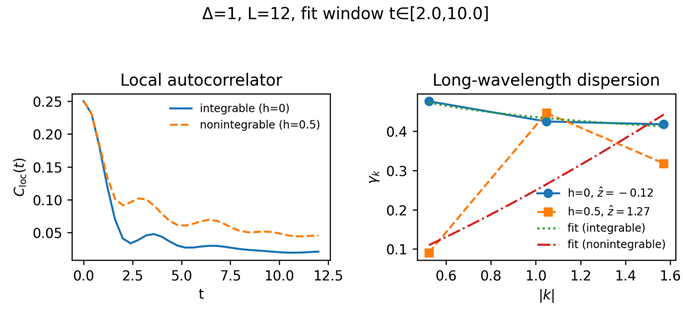
Concrete failure-mode example: a crossover regime where the single-mode hydrodynamic picture is not clean (multi-rate relaxation and integrability-induced structure). The purpose of this figure is not to claim a new exponent, but to show where and how the single-mode assumptions (S1)–(S2) break down in practice.

Numerical Benchmarks: ED with Conservative Uncertainty Quantification

We provide a reproducible pipeline (included in Supplementary File S2) that produces every figure from raw data. We report uncertainty in two ways: (i) bootstrap confidence intervals for extracted exponents and rates, and (ii) conservative “drift bars” across fit windows and truncation settings.

Exact Diagonalization Transport Extraction

We estimate the small-

k

decay rate

Γ (k)

from the time dependence of the spin structure factor

S (k, t)

, using linear fits of

l o g S (k, t)

over a window chosen by stability diagnostics.

Conservative Finite-Size Protocol.

Because a small number of

k

-points can mimic diffusion even when the true asymptotics are not diffusive, we enforce three guardrails. (i) We never infer diffusion from a single system size; Figure [fig:gamma] displays size drift explicitly. (ii) For each

L

we fit

Γ (k)

only on windows where the slope is stable under shifting the time-fit window used to extract

Γ

from

S (k, t)

. (iii) We report only an effective finite-size diagnostic

D_{e f f} (L) : = Γ (k_{m i n}) / k_{m i n}^{2}

(

k_{m i n} = 2 π / L

) together with its window-to-window drift; we do not extrapolate an infinite-volume diffusion constant from

L \leq 14

. This protocol is conservative by construction and is meant to avoid over-claiming hydrodynamic poles at

L \leq 14

.

Representative outputs are shown in Figure [fig:Deff] and, for visual context, in Figure [fig:gamma].

Conservative finite-size diagnostic

D_{e f f} (L) = Γ (2 π / L) / {(2 π / L)}^{2}

extracted from ED structure-factor decay rates at the smallest nonzero momentum. We report point estimates and bootstrap 95% CIs for two representative regimes in the XXZ chain: an integrable point (

h_{s t a g} = 0

) and a symmetry-breaking perturbation (

h_{s t a g} = 0.5

). The strong size drift and inconsistent scaling at

h_{s t a g} = 0

(integrable) illustrate the failure of a single diffusive description at these sizes; by contrast,

h_{s t a g} = 0.5

shows a comparatively stable

D_{e f f} (L)

across

L

.

$L$	$h_{s t a g}$	$D_{e f f} (L)$	95% CI
8	0.0	0.242	[0.106, 0.348]
10	0.0	1.661	[1.316, 1.962]
12	0.0	1.736	[1.443, 2.118]
14	0.0	1.409	[1.409, 1.409]
	0.5	0.303	[0.252, 0.354]
10	0.5	0.296	[0.294, 0.298]
12	0.5	0.330	[0.326, 0.334]
14	0.5	0.335	[0.335, 0.335]

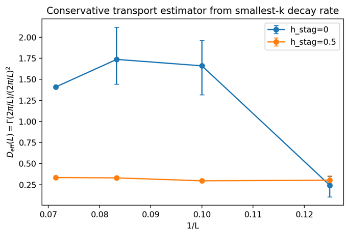
Referee-oriented “worst-case” transport summary at small sizes: the conservative estimator

D_{e f f} (L) = Γ (2 π / L) / {(2 π / L)}^{2}

shown against

1 / L

, with bootstrap 95% confidence intervals inherited from the decay-rate extraction. The pronounced drift and non-monotonicity at

h_{s t a g} = 0

illustrate why we avoid interpreting

L \leq 14

data as asymptotic diffusion in the integrable regime. The broken-integrability case

h_{s t a g} = 0.5

is comparatively stable across sizes, consistent with (but not a proof of) a diffusive window.

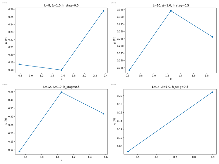
Transport extraction diagnostic across system sizes (XXZ chain with integrability broken by a staggered field

h = 0.5

). For each

L \in {8,10,12,14}

we estimate the decay rate

Γ (k)

for several discrete momenta

k_{n} = 2 π n / L

and report

Γ (k)

vs.

k^{2}

. Rather than relying on three-point linearity, we treat the small-

k

window as a size-dependent fit problem: we require stability of the slope under window shifts and propagate the resulting spread as a systematic uncertainty in

D_{e f f} (L)

and in the inferred

k^{2}

trend (Section [sec:numerics_protocol]).

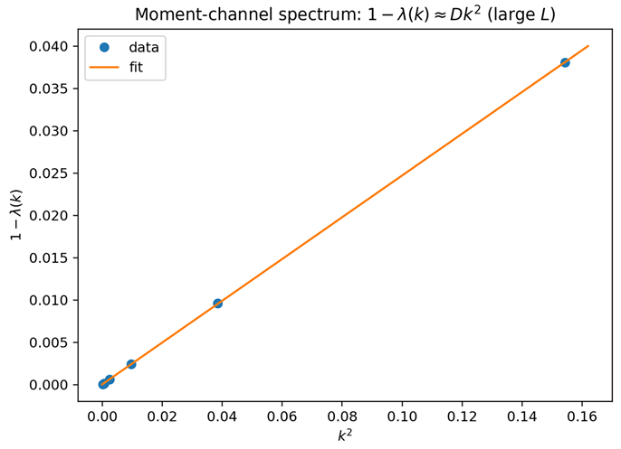
Illustrative small-

k

rate-versus-

k^{2}

diagnostic for a single system size. The plot is provided for visual context only: with few available momenta at

L \leq 14

, apparent linearity cannot be taken as asymptotic evidence for a diffusion pole. Consequently, the main text reports only the finite-size diagnostic

D_{e f f} (L) = Γ (2 π / L) / {(2 π / L)}^{2}

together with window-to-window drift (Table [tab:Deff]), and does not extrapolate an infinite-volume diffusion constant.

Conservative reporting. Because

L \leq 14

provides only a coarse momentum grid, we do not quote a single infinite-volume diffusion constant. Instead we report the finite-size diagnostic

D_{e f f} (L) = Γ (2 π / L) / {(2 π / L)}^{2}

and its drift across admissible fit windows. Supplementary File S2 contains the full set of window scans, slope-stability tests, and additional integrity checks used to decide which fits are admissible, including an explicit cross-

L

time-window sensitivity test (Supplementary Fig. S2.3).

Finite-Size Drift Diagnostics and the “Negative Exponent” Issue

An effective slope estimator

\hat{z} (L)

constructed from finite-size trends can yield nonphysical values (including negative numbers) in regimes where the hydrodynamic single-mode assumption is violated (e.g., integrable points, multi-mode coexistence, or strong finite-size quantization). For this reason we treat

\hat{z}

strictly as a breakdown diagnostic, not as a dynamic exponent, and we relegate the corresponding plots to Appendix [app:numerics] where they are clearly labelled as such.

TEBD/MPS Cross-Checks (Supplementary Only)

To reduce numerical-risk surface area in the main manuscript, all TEBD/MPS material is confined to Supplementary File S1 (including bond-dimension ladders, truncation thresholds, and time-step refinement). No main-text scaling claim relies on TEBD.

One-Page Synthesis of Regimes, Scalings, and Uncertainties

For ease of review, Table [tab:synthesis] collects the central operational claims, the dynamical regime in which they are supported, and the level of validation provided in this submission.

Synthesis: dynamics/regime

\times

transport diagnostic

\times

copy-time scaling. “Supported by” indicates what in this submission actually underwrites the stated scaling (theorem, exact toy model, or conservative ED estimate with confidence intervals).

Model / dynamics	Regime / structure	Diagnostic	$τ_{c o p y}$ scaling	Supported by
Gaussian charge field (commuting)	Diffusive kernel, Gaussian fluctuations	Exact TV distance [eq:tv_two_gaussians]	$\sim l^{2} / (4 D)$ (log- $η$ corr.)	Appendix [app:gaussian]
Chaotic $U (1)$ dynamics (generic)	Ballistic operator growth + diffusive charge	Separation Prop. [prop:separation]	$τ_{O T O C} \sim l$ , $τ_{c o p y} \sim l^{2}$	Prop. [prop:separation]
XXZ chain ( $h_{s t a g} = 0.5$ )	Nonintegrable, candidate diffusive window	$D_{e f f} (L)$ (bootstrap CI)	Consistent with $l^{2}$ window; no asymptotic claim	Table [tab:Deff], Fig. [fig:Deff]
XXZ chain ( $h_{s t a g} = 0$ )	Integrable / multimode	Drift/nonmonotone $D_{e f f} (L)$	Single-mode diffusion fails	Fig. [fig:Deff], Sec. [sec:numerics_protocol]
Range- $R$ QCA	Strict light cone	Hard causal delay	$τ_{c o p y} \geq ⌈ d / R ⌉$	Prop. [prop:qca_hard_bound]

Programmatic Outlook: QCA Locality and Operational Copy-Time Distances

This section is intentionally programmatic and nonessential. The journal-suitable results of the present manuscript are the operational definition, the minimal locality bounds, and the hydrodynamic closure statements supported by reproducible numerics (Sections 2–9). Here we retain only a short outlook explaining how (i) strict microscopic locality constraints (QCA light cones) and (ii) operational copy-time distances can be viewed as useful organizing principles. More speculative directions (index-theoretic classification, code-subspace constraints, and any gravity-facing remarks) have been removed from the main text and deferred to the author’s separate preprints for interested readers. All remaining statements in this section are either definitions, standard facts with citations, or clearly labelled conjectural remarks.

Locality-Preserving QCA as a Clean Microscopic Substrate

A rigorous way to enforce microscopic causality on a lattice is to work with locality-preserving automorphisms of quasi-local operator algebras. In one dimension, this is the standard definition of a reversible QCA [13,14,15].

[13,14,15] Let

A = \bar{⋃_{Λ \subset Z f i n i t e} A_{Λ}}

be the quasi-local

C^{*}

-algebra generated by finite-region matrix algebras

A_{Λ}

. A reversible QCA of range

R

is a

*

-automorphism

α : A \to A

such that for every finite region

Λ

,

α (A_{Λ}) \subseteq A_{Λ^{+ R}},

where

Λ^{+ R}

is the

R

-neighborhood of

Λ

in the lattice metric. Equivalently,

α

maps any observable supported on

Λ

to an observable supported on

Λ^{+ R}

.

In contrast to Hamiltonian LR bounds (which have exponential tails), a range-

R

QCA has a strict light cone: after

t

discrete steps, support enlarges by at most

R t

.

Let

α

be a reversible QCA of range

R

and let

ρ_{\pm} (0)

be two global states that coincide on

A^{c}

. Then for any receiver region

B

with

d (A, B) > R t

,

ρ_{+, B} (t) = ρ_{-, B} (t) \Rightarrow {A d v}_{A \to B} (t) = 0,

hence

τ_{c o p y} (A \to B; η) \geq ⌈ d (A, B) / R ⌉

for any

η > 0

.

Copy-Time Distances and an Operational Geometry

Given a family of regions and a fixed

η

, the copy time defines a directed operational “distance”

d_{η} (A, B) : = τ_{c o p y} (A \to B; η),

with a natural symmetrization

d_{η}^{s y m} (A, B) : = m a x {d_{η} (A, B), d_{η} (B, A)}

. In strictly causal systems (e.g., QCAs),

d_{η}

is bounded below by the light-cone distance (Proposition [prop:qca_hard_bound]). In transport-dominated phases with conservation laws,

d_{η}

instead probes the geometry of hydrodynamic modes (Sections 4–6).

A basic consistency check for any “emergent geometry” interpretation is that

d_{η}^{s y m}

behaves approximately like a metric at scales where the effective theory is local. Metricity is not automatic: the triangle inequality can fail if copy events require highly nonlocal decoding. A conservative stance is therefore to treat

d_{η}

as an operational causal preorder rather than a metric and to ask under what dynamical restrictions it becomes approximately metric.

How microscopic structure controls copy-time geometry (outlook).

Microscopic structure	Dominant control of $τ_{c o p y}$	Geometric interpretation of $d_{η}$
Range- $R$ QCA (strict cone)	Hard causal delay $≳ d / R$	Operational causal cone; metricity requires extra mixing
Local Hamiltonian (LR tails)	Exponential tail outside cone	Approximate causal cone with exponentially small leakage
Conservation + diffusion	Slowest mode $D k^{2}$ (Theorem [thm:main_single])	Transport geometry; distances can scale as $l^{2}$ in a diffusive window
Integrable / ballistic channels	Coexisting modes, Drude weight	Breakdown of single-mode geometry; $d_{η}$ is model dependent
Code-subspace restriction	Admissible perturbations/observables	Geometry depends on code constraints and decoding locality

Schematic: sender region

A

creates a weak perturbation; receiver region

B

certifies it via hypothesis testing, defining

τ_{c o p y} (A \to B; η)

. This figure is illustrative only and does not enter any bound or numerical inference.

Conclusions

We introduced a receiver-limited operational definition of copy time, proved minimal locality bounds, and derived a hydrodynamic susceptibility control theorem under explicit (and potentially fragile) assumptions about single-mode diffusive closure. Our numerical benchmarks in the XXZ chain are deliberately conservative: they provide finite-size transport diagnostics with uncertainty quantification and illustrate consistency checks, but they do not establish asymptotic scaling or extract an infinite-volume diffusion constant. Throughout, we emphasize failure modes (integrability, multi-mode coexistence, localization, and nonconserving dynamics) where the hydrodynamic closure is expected to break down. A short, nonessential outlook on QCA locality and operational copy-time distances is included for context but is not used to justify any theorem or numerical claim.

Proof Sketches and Technical Details

Proof of Theorem [thm:lr_upper]

We treat the Hamiltonian/Lindbladian Lieb–Robinson-tail case (H); the strict circuit/QCA light-cone statement (C) follows immediately from [eq:LR_C] because the evolved observable remains supported in

A^{+ R t}

and therefore cannot influence

B

when

d (A, B) > R t

. Let

δ ρ (0) = ρ_{+} (0) - ρ_{-} (0)

and

δ ρ_{B} (t) = {T r}_{B^{c}} (U_{t} (δ ρ (0)))

. By duality of the trace norm,

2 {A d v}_{A \to B} (t) = ∥ δ ρ_{B} (t) ∥_{1} = \underset{∥ O_{B} ∥_{\infty} \leq 1}{s u p} T r (O_{B} δ ρ_{B} (t)) = \underset{∥ O_{B} ∥_{\infty} \leq 1}{s u p} T r (O_{B} (t) δ ρ (0)),

where

O_{B} (t) = U_{t}^{†} (O_{B})

is the Heisenberg evolution. Since

δ ρ (0)

is supported on

A

, insert an arbitrary operator

O_{B}^{(A^{c})} (t)

supported on

A^{c}

and use

T r (O_{B}^{(A^{c})} (t) δ ρ (0)) = 0

:

T r (O_{B} (t) δ ρ (0)) = T r ((O_{B} (t) - O_{B}^{(A^{c})} (t)) δ ρ (0)) .

Choosing

O_{B}^{(A^{c})} (t)

as the best approximation to

O_{B} (t)

supported on

A^{c}

and applying standard LR localization bounds yields

\underset{s u p p (Y) \subseteq A^{c}}{i n f} ∥ O_{B} (t) - Y ∥_{\infty} \leq C_{1} e^{- μ (d (A, B) - v t)} .

Finally,

|T r (X δ ρ (0))| \leq ∥ X ∥_{\infty} ∥ δ ρ (0) ∥_{1}

with

∥ δ ρ (0) ∥_{1} \leq 2

gives

2 {A d v}_{A \to B} (t) \leq 2 C_{1} e^{- μ (d (A, B) - v t)},

which is [eq:lr_finish].

Hydrodynamic Single-Mode Derivation

From Projected Dynamics to a Diffusion Pole

In the single-mode window, the projected Liouvillian on the conserved-density subspace is diagonal in Fourier space and has eigenvalues

- Γ (k)

with

Γ (k) = D k^{2} + o (k^{2})

. Let

δ q_{k} (t)

denote the conserved-density mode. Then

δ q_{k} (t) = e^{- Γ (k) t} δ q_{k} (0)

. The receiver observable

J_{B}

couples to these modes with form factor

F_{B} (k)

, so the projected signal takes the form

S_{B} (t) = ϵ \sum_{k \neq 0} F_{B} (k) e^{- Γ (k) t} δ q_{k} (0) + (higher modes) .

The second-moment susceptibility in Definition [def:chi2] is essentially the

k

-space weighted sum

\sum_{k \neq 0} {|F_{B} (k)|}^{2} / Γ {(k)}^{2}

, which is dominated by the smallest

|k|

in finite volume.

Threshold Inversion and $l^{2}$ Scaling

For a localized sender perturbation,

δ q_{k} (0) \sim e^{- i k x_{A}}

and for an interval receiver

B

centered at

x_{B}

,

F_{B} (k) \sim e^{i k x_{B}} s i n c (k w / 2)

. Thus the signal depends on

x_{B} - x_{A} = l

through an oscillatory factor

e^{i k l}

. In the continuum approximation, replacing the discrete sum by an integral yields the heat-kernel expression [eq:heat_kernel] and the saddle-point estimate [eq:signal_scaling], from which [eq:tau_scaling] follows. Finite-volume corrections can be bounded by Poisson summation and yield the explicit

O (l o g (1 / η))

threshold term quoted in Theorem [thm:main_single].

We provide the diffusion-kernel computation leading to [eq:tau_scaling]. In one dimension, a localized chemical potential profile evolves as

δ μ (x, t) \approx {(4 π D t)}^{- 1 / 2} e x p (- x^{2} / (4 D t))

in the hydrodynamic window. Evaluating its overlap with a receiver region at distance

l

yields a signal proportional to

e x p (- l^{2} / (4 D t))

, leading to

τ \sim l^{2} / (4 D)

up to logarithmic threshold factors.

Moment-Channel Optimality in Gaussian Fluctuation Algebras

We show that if the induced reduced states on

B

are Gaussian in the relevant fluctuation variables, then low moments determine the Helstrom measurement asymptotically, and the moment-channel lower bound [eq:moment_lower] matches

A d v

to leading order.

QCA Locality Versus LR Tails and Index Sensitivity

From Strict Causal Cones to Operational Zero Advantage

For a range-

R

QCA, the strict light cone implies an exact vanishing statement: for any observable

O_{B}

supported on

B

and any operator

X_{A}

supported on

A

,

T r (O_{B} α^{t} (X_{A})) = 0 whenever d (A, B) > R t,

because

α^{t} (X_{A})

is supported on

A^{+ R t}

and the local algebras commute at distance. In contrast, for Hamiltonian evolution one only obtains exponentially small commutator tails as in [eq:LR_H]. This distinction matters operationally: in QCA dynamics,

{A d v}_{A \to B} (t)

is exactly zero outside the cone, whereas for Hamiltonians it is merely exponentially small and can in principle accumulate via many weak channels.

Why Copy-Time Data Might “See” the Index

The QCA index [14] is defined through support-algebra dimensions associated with the image of local algebras under

α

. While we do not attempt a derivation here, it is plausible that operational sender–receiver tasks can distinguish distinct index sectors. A concrete approach is to compare

d_{η}

for families of disjoint sender/receiver intervals under stacking and coarse graining, testing multiplicativity patterns implied by the index. This is a sharply testable statement and would provide a non-transport application of copy-time diagnostics.

Finite-Size Corrections for Diffusion-Kernel Inversion

Here we record a finite-size bound that turns the heuristic replacement of a discrete

k

-sum by a continuum integral into a controlled approximation.

Let

k_{n} = 2 π n / L

,

n \in Z

, and consider the kernel

K_{L} (l, t) : = \frac{1}{L} \sum_{n \neq 0} e^{- D k_{n}^{2} t} e^{i k_{n} l} .

By Poisson summation, for

t D ≪ L^{2}

one has

K_{L} (l, t) = \frac{1}{\sqrt{4 π D t}} \sum_{m \in Z} e x p (- \frac{{(l + m L)}^{2}}{4 D t}) - \frac{1}{L},

where the

- 1 / L

subtracts the zero mode. The leading term

m = 0

recovers the infinite-line heat kernel [eq:heat_kernel]; the finite-size correction is bounded by

|K_{L} (l, t) - \frac{1}{\sqrt{4 π D t}} e^{- l^{2} / (4 D t)}| \leq \frac{2}{\sqrt{4 π D t}} \sum_{m \geq 1} e x p (- \frac{{(m L - l)}^{2}}{4 D t}) + \frac{1}{L} .

For

l \leq L / 2

and

t D \leq κ L^{2}

with

κ < 1 / 16

, the dominant correction is

O (e^{- {(1 - 2 l / L)}^{2} / (16 κ)})

, exponentially small in

1 / κ

. This justifies using the continuum inversion for

τ_{c o p y}

in the pre-asymptotic window

t ≪ L^{2} / D

.

Gaussian Discrimination and Moment Sufficiency: An Explicit Bound

Assume that, in the hydrodynamic window, the receiver’s relevant fluctuation variable

X_{B}

(e.g., coarse-grained charge in

B

) is approximately Gaussian under both hypotheses, with means

\pm m (t)

and common variance

σ^{2} (t)

. Then the optimal Helstrom measurement reduces (in the classical limit) to thresholding

X_{B}

, and the resulting advantage is

A d v (t) \approx T V (N (m (t), σ^{2} (t)), N (- m (t), σ^{2} (t))) = e r f (\frac{m (t)}{\sqrt{2} σ (t)}) .

For small signal-to-noise ratio

m / σ

,

A d v (t) \sim \sqrt{\frac{2}{π}} \frac{m (t)}{σ (t)}

. Since

m (t)

is controlled by the diffusion kernel [eq:signal_scaling] and

σ (t)

is set by equilibrium fluctuations, low moments (mean and variance) are sufficient to determine the advantage at leading order. This provides a principled route to moment-channel near-optimality in regimes where the fluctuation algebra is approximately Gaussian.

Additional Numerical Tables and Metadata

Finite-size “effective-exponent” diagnostics (including negative/drifting slopes at the integrable point) are provided as CSV tables in Supplementary File S2; in the main PDF we treat these quantities strictly as breakdown diagnostics rather than physical exponents.

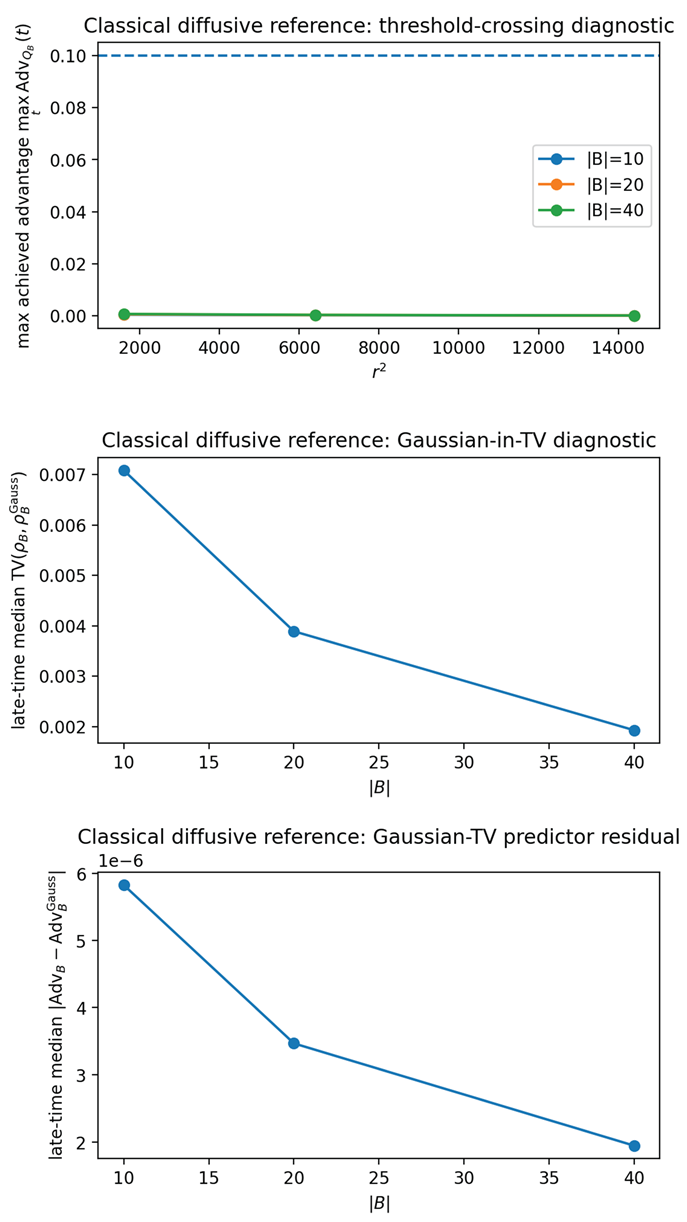
Selected pipeline diagnostics (Appendix). Top: a threshold-crossing diagnostic for the classical diffusive reference at

η = 0.1

(dashed line), showing that for this conservative parameter set the receiver advantage stays below threshold, hence

τ_{c o p y} = \infty

(no crossing) while

{m a x}_{t} A d v

remains small. Middle: Gaussian approximation error (trace-distance proxy) versus receiver size. Bottom: predictor residual versus receiver size for a regression-based proxy. The full diagnostic set (including parameter sweeps) is included in Supplementary File S2 (Appendix [app:repro]).

Supplementary File S2 provides additional numerical diagnostics and reporting details (including window scans and stability checks) used to assess the single-mode window at the accessible sizes. We recommend interpreting small-

L

“effective exponents” only as diagnostics of hydrodynamic breakdown, not as physical exponents in integrable regimes.

Reproducibility Checklist and Run Manifest

For reproducibility, Supplementary Files S1–S4 and the Supplementary Code Archive SC1 include:

a self-contained description of the numerical protocols (ED and TEBD/MPS checks) and parameter registries (Supplementary File S1);
additional integrity checks, fit-window scans, and diagnostic plots supporting the transport-extraction procedure (Supplementary File S2);
extended, referee-auditable derivations of the key inequalities and conditional closure assumptions (Supplementary File S3);
an explicit positioning/taxonomy relative to nearby diagnostics together with toy examples that separate QICT from operator-growth diagnostics (Supplementary File S4);
the minimal code/data/environment bundle used to generate the reported ED diagnostics and figure post-processing at the studied sizes (Supplementary Code Archive SC1).

Pseudo-Code for the ED Extraction

To keep the main PDF within a standard length while preserving full reproducibility, we move the complete pseudo-code listing (including parameter registries and metadata logging) to Supplementary File S1 (supplementary_pseudocode.tex) included in the submission package. The numerical protocols and all reported figures remain fully specified in the main text and Appendix [app:numerics].

Pseudo-Code for TEBD Convergence

The full TEBD/MPS convergence pseudo-code and refinement checklist (bond-dimension ladder, truncation thresholds, and time-step refinement) are provided in Supplementary File S1 (supplementary_pseudocode.tex). We emphasize that all TEBD-based statements in the main text are restricted to regimes where stability checks are satisfied within reported uncertainties.

Supplementary Materials

Supplementary File S1: numerical protocols, pseudo-code, and TEBD/MPS stability checks. Supplementary File S2: additional transport-extraction diagnostics, window scans, and supporting plots. Supplementary File S3: extended derivations and conservative error controls for the operational and hydrodynamic layers. Supplementary File S4: positioning relative to existing diagnostics and toy examples separating receiver-limited certifiability from operator growth. Supplementary Code Archive SC1: code, environment files, and minimal data needed to reproduce the ED diagnostics and figure post-processing at the studied sizes.

References

Helstrom, Carl W. Quantum detection and estimation theory; 1976. [Google Scholar]
Holevo, A.S. Statistical decision theory for quantum systems. Journal of Multivariate Analysis 1973, 3(4), 337–394. [Google Scholar] [CrossRef]
Lieb, Elliott H.; Robinson, Derek W. The finite group velocity of quantum spin systems. Communications in Mathematical Physics 1972, 28(3), 251–257. [Google Scholar] [CrossRef]
Bravyi, S.; Hastings, M. B.; Verstraete, F. Lieb–robinson bounds and the generation of correlations and topological quantum order. Physical Review Letters 2006, 97, 050401. [Google Scholar] [CrossRef] [PubMed]
Kubo, R. Statistical-mechanical theory of irreversible processes. I. General theory and simple applications to magnetic and conduction problems. Journal of the Physical Society of Japan 1957, 12(6), 570–586. [Google Scholar] [CrossRef]
Mori, H. Transport, collective motion, and brownian motion. Progress of Theoretical Physics 1965, 33(3), 423–455. [Google Scholar] [CrossRef]
Zwanzig, R. Memory effects in irreversible thermodynamics. Physical Review 1961, 124, 983–992. [Google Scholar] [CrossRef]
Nahum, Adam; Vijay, S.; Haah, Jeongwan. Operator spreading in random unitary circuits. Physical Review X 2018, 8, 021014. [Google Scholar] [CrossRef]
von Keyserlingk, C. W.; Rakovszky, Tibor; Pollmann, Frank; Sondhi, S. L. Operator hydrodynamics, OTOCs, and entanglement growth in systems without conservation laws. Physical Review X 2018, 8, 021013. [Google Scholar] [CrossRef]
Xu, Shenglong; Swingle, Brian. Scrambling dynamics and out-of-time-ordered correlators in quantum many-body systems. PRX Quantum 2024, 5, 010201. [Google Scholar] [CrossRef]
Khemani, Vedika; Vishwanath, Ashvin; Huse, David A. Operator spreading and the emergence of dissipative hydrodynamics under unitary evolution with conservation laws. Physical Review X 2018, 8, 031057. [Google Scholar] [CrossRef]
Rakovszky, Tibor; Pollmann, Frank; von Keyserlingk, C. W. Diffusive hydrodynamics of out-of-time-ordered correlators with charge conservation. Physical Review X 2018, 8, 031058. [Google Scholar] [CrossRef]
Schumacher, Benjamin; Werner, Reinhard F. Reversible quantum cellular automata; 2004. [Google Scholar]
Gross, D.; Nesme, V.; Vogts, H.; Werner, R. F. Index theory of one dimensional quantum walks and quantum cellular automata. Communications in Mathematical Physics 2012, 310, 419–454. [Google Scholar] [CrossRef]
Arrighi, P.; Nesme, V.; Werner, R. Unitarity plus causality implies localizability. Journal of Computer and System Sciences 2019, 101, 26–40. [Google Scholar] [CrossRef]

Disclaimer/Publisher’s Note: The statements, opinions and data contained in all publications are solely those of the individual author(s) and contributor(s) and not of MDPI and/or the editor(s). MDPI and/or the editor(s) disclaim responsibility for any injury to people or property resulting from any ideas, methods, instructions or products referred to in the content.

© 2026 by the authors. Licensee MDPI, Basel, Switzerland. This article is an open access article distributed under the terms and conditions of the Creative Commons Attribution (CC BY) license (http://creativecommons.org/licenses/by/4.0/).

Copyright: This open access article is published under a Creative Commons CC BY 4.0 license, which permit the free download, distribution, and reuse, provided that the author and preprint are cited in any reuse.

Quantum Information Copy Time (QICT): Operational Definition, Minimal Locality Bounds, Hydrodynamic Susceptibilities, and a Programmatic Outlook

Abstract

Keywords:

Subject:

Introduction

Operational Definition and Preliminaries

Copy Time as Receiver-Limited Hypothesis Testing

Elementary Bounds and Caveats

Minimal Locality Bounds and What Is Genuinely Nontrivial

Locality-Preserving Dynamics and Lieb–Robinson Constraints

Conservation Laws and an Explicit Receiver Class

Hydrodynamic Closure: From Charge Bias to Spectral Susceptibility

Setup: local equilibrium manifold and linearization

A Principled Definition of the Second-Moment Susceptibility

Two Theorems: Minimal and Single-Mode

Worked Hydrodynamic Example: One-Dimensional Diffusion Kernel

Linear-Response Form of the Reduced-State Difference

Diffusion Equation for the Conserved Density

Receiver Signal and a Concrete Threshold-to-Time Relation

An Exactly Solvable Gaussian Diffusion Toy Model (Fully Analytic)

Moment-Channel Approximation and Operational Accessibility

Definition of the Moment Channel

When Moment Restriction Is Asymptotically Optimal

Copy Time Versus OTOCs and Lieb–Robinson Bounds: A Sharp Separation

Ballistic Operator Growth Does Not Imply Fast Copying Under Conservation

Proof Sketch.

Relation to LR Bounds

Failure Modes and Boundaries of Validity

Numerical Benchmarks: ED with Conservative Uncertainty Quantification

Exact Diagonalization Transport Extraction

Conservative Finite-Size Protocol.

Finite-Size Drift Diagnostics and the “Negative Exponent” Issue

TEBD/MPS Cross-Checks (Supplementary Only)

One-Page Synthesis of Regimes, Scalings, and Uncertainties

Programmatic Outlook: QCA Locality and Operational Copy-Time Distances

Locality-Preserving QCA as a Clean Microscopic Substrate

Copy-Time Distances and an Operational Geometry

Conclusions

Proof Sketches and Technical Details

Proof of Theorem [thm:lr_upper]

Hydrodynamic Single-Mode Derivation

From Projected Dynamics to a Diffusion Pole

Threshold Inversion and l 2 Scaling

Moment-Channel Optimality in Gaussian Fluctuation Algebras

QCA Locality Versus LR Tails and Index Sensitivity

From Strict Causal Cones to Operational Zero Advantage

Why Copy-Time Data Might “See” the Index

Finite-Size Corrections for Diffusion-Kernel Inversion

Gaussian Discrimination and Moment Sufficiency: An Explicit Bound

Additional Numerical Tables and Metadata

Reproducibility Checklist and Run Manifest

Pseudo-Code for the ED Extraction

Pseudo-Code for TEBD Convergence

Supplementary Materials

References

MDPI Initiatives

Important Links

Subscribe

Threshold Inversion and $l^{2}$ Scaling