
Submitted:
03 January 2026
Posted:
05 January 2026
You are already at the latest version
Abstract
Wastewater is an abundant yet underutilized source of thermal energy. Integrating wastewater flow with heat exchangers and heat pumps is a promising method for addressing buildings' heating and cooling requirements. This approach not only enhances energy efficiency but also promotes sustainability in buildings. This study explores the techno-economic and environmental potential of such a system, known as a Wastewater Energy Transfer (WET) system. An energy model was developed to simulate and compare the performance of a WET system with an existing conventional Heating, Ventilation and Air Conditioning (HVAC) system. Using local greenhouse gas (GHG) emissions factors, utility rates, and weather data, the model calculated both systems' comparative energy consumption, operating costs, and GHG emissions. The models were created to determine the project's economic and environmental viability. Toronto Metropolitan University (formerly Ryerson University) campus buildings were utilized for a case study and implementation of a WET system. The analysis included six Canadian cities of Halifax, Montreal, Toronto, Winnipeg, Calgary, and Vancouver, with varying climates and energy infrastructures. Montreal had the highest operating cost savings at $2,057,855, while Calgary had the lowest at $128,544. Winnipeg led in GHG reductions, offsetting 5,464 tonnes annually, whereas Montreal had the smallest reduction at 21 tonnes.
Keywords:
wastewater
; heat pump
; heat exchanger
; modelling and simulation
; feasibility Analysis
1. Introduction
The building sector is one of Canada's largest contributors to greenhouse gas (GHG) emissions, primarily due to high heating demands and reliance on fossil fuels. With 82% of electricity generated in Canada coming from non-GHG-emitting sources, widespread electrification for heating could significantly reduce building’s environmental footprint [1,2]. Various electric driven heat pump technologies have been promoted, but their widespread implementation has been relatively slow [3,4]. The primary reason for this trend can be attributed to Canada's comparatively low natural gas prices. Additionally, the relatively high cost of electric heat pumps serves to reduce the financial incentives for adopting these newer technologies. The challenge is to develop clean and financially viable solutions that reduce or eliminate dependence on fossil fuels and minimize the carbon footprint [5]. This study aims to thoroughly examine the techno-economic and environmental potentials of the Wastewater Energy Transfer (WET) system in the context of Canadian conditions [6].
One underutilized source of carbon-free renewable energy available in urban areas is sewer's wastewater. The first WET systems were constructed in 1980 in Germany, Switzerland and Scandinavian countries [7], and while the number of installations has slowly increased throughout Europe and China, the technology in general remains underutilized [8]. Approximately 90% of the thermal energy used for domestic hot water is lost down the drain, which the United States Department of Energy estimates to be around 235 billion kWh of thermal energy each year [9]. On average, about 40% of the heat generated in a city is lost to the sewer system [8]. Wastewater is an abundant resource of thermal energy in urban settings. The average household in Toronto consumes approximately 630 L of water per day [10], with a total of 3.2 billion m3 of water annually across Canada [11] makes its way to the sewer systems, this represents a large carbon-free source of renewable thermal energy. Much of this energy can be recovered through properly designed heat exchangers and heat pump systems. In one of the studies [8] on these systems concluded that the largest challenges in the design and operations are overcoming the impact of clogging and biofouling on the performance of the heat exchangers.
WET systems utilize heat exchangers and heat pumps to extract thermal energy from the wastewater flowing through sewers [12]. While various configurations exist, the typical process involves diverting wastewater from the sewer into a screening station, where large solids and particulates are filtered out. The screened wastewater is then pumped to a heat exchanger that transfers thermal energy to a heat pump using an intermediary working fluid. With wastewater temperatures around 20°C year-round [13], WET systems capitalize on this relatively warm wastewater as a carbon-free heat source during winter, serving as a cool heat sink in summer. This temperature consistency makes wastewater an ideal candidate for use with heat pump system.
Most of these systems are installed in Europe, with a notable example being the Munich University Hospital in Munich, Germany [14]. This installation has been operating since it was set up in 2014. The system uses wastewater generated by the hospital, and due to the high volumes of steam used for disinfection and sanitation, the average temperature of the wastewater supplied to the WET system is approximately 50°C. Another installation is found in a 28-storey, 22,000 m2 office tower in Winterthur, Switzerland [15], which connects to a nearby main interceptor sewer. This system utilizes approximately 160 L/s of wastewater and has a heating capacity of 590 kW and a cooling capacity of 600 kW. In most installations, the temperature of the wastewater typically ranges from 10°C to 20°C, with a standard coefficient of performance (COP) between 5 and 6.
In North America, there are two prominent installations of note: one is located in Quebec City, Canada [16], and the other is in Washington, D.C., United States [17]. The installation in Quebec City is part of a residential development and has a capacity of 322 kW. The installation in Washington, D.C., is located at the American Geophysical Union (AGU), a not-for-profit organization dedicated to the advancement of the sciences. The success of the North American installations demonstrated that these systems can be a viable alternative; however, their techno-economic viability still needs to be fully understood.
Most WET installations are in Europe, where energy prices are significantly higher than in North America [18]. Additionally, carbon pricing has been implemented in the EU since 2005. These conditions enhance the financial viability of these systems in European countries. In North America, where energy prices are generally lower, and carbon pricing is not widely adopted, the economic feasibility of WET systems has yet to be established, which is one of the intended goals of this study.
The Toronto Water Department provided typical temperature data for a large sewer in Toronto, Canada, covering the period from August 8, 2018 to October 29, 2019 [19]. This data was aggregated to create an average daily temperature profile, as shown in Figure 1. The average temperature of the sewer was recorded at 24.4°C, which is higher than the typical temperatures reported in the literature. This elevated temperature range allows WET systems to operate heat pumps with a higher COP, making them more energy-efficient and environmentally friendly compared to conventional alternatives.
WET systems require a reliable source of wastewater to operate. In addition to considering water temperature, research indicates that average wastewater flow rates are generally stable throughout the year. However, it is important to note that these flow rates can vary during different times of the day. Flow data was obtained for various locations throughout the City of Toronto from the Toronto Water Department and was compiled to generate average daily flow graphs for each sewer (Figure 1). The sewers undergo predictable flow rates, with the minimum flow rates occurring in the early morning, and peaks in the morning hours and in the evening. It is vital to understand the minimum flow rate in each sewer when sizing and designing a WET system.
This study uses the Toronto Metropolitan University (TMU) campus buildings as a case study to evaluate the techno-economic viability of WET systems for a district energy system in Toronto, Canada. The TMU district energy systems are well-equipped to integrate multiple energy sources along with heating and cooling demands, optimizing operations for maximum economic benefit. The TMU analysis is being extended to encompass additional major cities throughout Canada in order to assess the impact of local climatic conditions on such systems.
2. WET System, Methodology, Results
2.1. WET System Configuration
Figure 2 illustrates the study configuration of a WET system using a shell-and-tube heat exchanger connection with wastewater [20,21]. This design effectively addresses some of the challenges associated with these systems operation, particularly the need for a reliable method to screen and remove solids from the wastewater stream. The design incorporates a cleaning screen and a built-in auger assembly system. The components of this design include a wetwell, which houses the screen and auger assembly, heat pump, and other supporting elements. Wastewater flows by gravity into the wetwell, which has a vertical shaft constructed adjacent to the sewer line. The connection to the wetwell is located near the bottom of the sewer, allowing a significant portion of the wastewater to enter while minimizing the amount of sand and debris that also gets drained. At Point 2, a cleaned screen and auger assembly remove large particles from the wastewater. The screened wastewater collects at the bottom of the wetwell. Auger lifts the filtered solids within the screen assembly, as indicated at Point 6. Once the solids reach the top of the screen assembly, they are discharged back into the sewer along with the wastewater (Point 7). The screened wastewater from the bottom of the wetwell, noted at Point 2, is then pumped to the WET heat exchanger (HX) at Point 3. The Wastewater Heat Exchanger (WET HX) is a shell-and-tube heat exchanger, with the screened wastewater flowing through the shell side and clean water flowing through the tube side. During this heating process, thermal energy is transferred from the wastewater to the clean water, which is then supplied to a heat pump, and the process will be vice versa in cooling mode.
As mentioned, the TMU campus was chosen as a case study for the feasibility evaluation of the WET system. TMU campus contain several large buildings with high annual heating and cooling loads. Furthermore, they also have a large number of occupants, as well as computers and equipment, that all result in large year-round base heating and cooling demands. The campus is located within cities, ensuring the presence of a sizable sewer in the vicinity. The proposed WET system (Figure 2) can provide the base heating and cooling loads, serving as the primary supply source. Conventional Heating, Ventilation and Air Conditioning (HVAC) systems will supply the remaining thermal demands. The proposed TMU hybrid system ensures that the high capital investment required for the WET system has a high utilization rate, maximizing operating savings and improving financial returns.
2.2. Methodology
The adopted methodology can be divided into three main sections: 1) Building Load Modeling, 2) Equipment Modeling, and 3) Financial Modeling.
Building energy models were obtained for 16 buildings of TMU, taking into account each building's geometry, materials, HVAC details, and occupancy schedules [22,23]. These models were used to simulate hourly heating and cooling profiles of each building. The equipment for the conventional HVAC systems was modelled to determine the systems' electricity, natural gas, and water consumption, GHG emissions and operating costs. The equipment for the WET-hybrid systems was modelled, and the energy consumption, GHG emissions, and operating costs were assessed and compared to those of the conventional HVAC systems. Subsequently, a financial model was developed to evaluate the project returns for WET-hybrid system compared to the conventional system. This analysis aimed to determine the feasibility of such a system in the TMU-type situations in Toronto and the other chosen Canadian cities.
The models were simulated in Carrier HAP software [24] using weather files of Toronto and other Canadian cities [25]. Besides Toronto, the chosen cities were Halifax, Montreal, Winnipeg, Calgary, and Vancouver. These cities were chosen because they are among Canada's largest metropolitan centers and represent various climates and energy price structures. Figure 3 outlines the adopted process for this study.
2.1.1. Energy Prices and Emissions Factors
Table 1 compares the average costs of electricity and natural gas across selected cities in Canada. It also includes the GHG emission factors for electricity and natural gas per unit of energy.
For each city, the unit cost of energy for natural gas is several times lower than that of electricity. This disparity makes it financially challenging to transition from natural gas-based heating to electric in most parts of Canada. One potential solution is the use of heat pumps, which can provide more thermal energy than they require electrical energy as an input. In 4 of the 6 cities shown in Table 1, the GHG emissions per unit of energy are significantly lower for electricity than for natural gas. The cities where natural gas had lower GHG emissions per unit of energy than electricity were Halifax (Nova Scotia) and Calgary (Alberta). Therefore, transitioning from natural gas-based heating to heat pump-based electric heating is a considerable environmental benefit.
2.3. Building Modelling
The Heating Degree Days (HDD) and Cooling Degree Days (CDD) values were calculated using Canadian Weather data files with a reference temperature of 18°C. Figure 4 shows the annual HDD and heating demand, along with the annual CDD and cooling demand for the chosen cities.
A summary of the building energy demands for each city is given in Table 2. In addition to using each city’s unique weather, utility rates were also included for electricity, natural gas and water for each respective city. For Montreal and Toronto, two different electricity rates would be applicable to customers of this size.
For Montreal, the applicable electrical rates are LG and G9, whereas for Toronto the rates are Class A and Class B. In the following sections, both sets of electrical rates are considered and are labelled as Montreal (LG), Montreal (G9), Toronto (Class A) and Toronto (Class B).
A breakdown of the energy consumption, operating costs, and GHG emissions of the conventional systems are shown in Table 3 for each of the cities. The local electricity emissions factors were used in this analysis, as well as a natural gas emissions factor of 1.89 kg/m3 [31].
As seen in Table 3, the average annual operating cost was $1,858,824, with Vancouver having the lowest at $898,813 and Toronto (Class A) having the highest at $3,230,159. The average annual water consumption by the evaporative cooling towers was 55,459 m3, with the lowest being Calgary with 40,628 m3, and Montreal being the highest at 68,916 m3. The average annual GHG emissions was 4,507 tonnes. The largest GHG emissions resulted in Calgary with 7,453 tonnes was due to having the second coldest climate of the cities considered as well as the highest GHG emissions factor for electricity. Montreal exhibited the lowest GHG emissions, amounting to only 30 tonnes. This is primarily a result of the adoption of electric resistance boilers in place of natural gas systems. Furthermore, Montreal possesses the lowest electrical GHG emissions factor among the cities examined, emphasizing its sustainable energy.
2.4. WET System Equipment Modelling
A detailed model was developed in Excel to calculate and compare the energy consumption performance of a conventional HVAC system with a WET system. The conventional HVAC system serves as the baseline for comparative analysis. The WET system will be combined with conventional equipment to reduce capital costs and enhance its financial viability. The operating cost savings from the WET system will help offset the high initial capital investment required for the technology to be financially viable. As mentioned, the WET system will act as the primary heating and cooling source, while the conventional system will be used to meet peak demand. This approach limits the capacity and capital expenditure of the WET system but allows for its high utilization, enabling it to benefit from lower operating costs.
2.4.1. WET Heat Exchanger
The shell-and-tube type WET heat exchangers (WET HXs) [32] considered in this study can flow up to 16 L/s of clean water on the tube side and 32.6 L/s of wastewater on the shell side (Figure 5). An effectiveness curve, as shown in Figure 6, was obtained as a function of tube side flow rate for the wastewater flow rate at shell side of 32.6 L/s. When the installed capacity of the WET system exceeds the thermal demands of the campus buildings, the flow rate of the clean condenser water through the WET HXs is reduced which improves the effectiveness of the heat exchangers and provides the heat pumps with more favorable water temperatures.
The heat transferred across a WET HX is calculated as [23]:
where is the heat transferred in kW, is the tube side flow rate in kg/s, is the specific heat of water, is the temperature of the wastewater in °C, is the temperature of the intermediary fluid leaving the heat pump and flowing to the WET HX in °C, and is the effectiveness of the heat exchanger, as obtained from Figure 6.
The temperature of the intermediary fluid leaving the heat exchanger to the heat pump is calculate as [23]:
where is the temperature of the intermediary fluid leaving the heat pump going to the heat exchanger in °C.
The power draw of the wastewater supply pump is calculated as [23]:
where is the total flow rate of wastewater or 32.6 L/s per WET HX, is the wastewater pump head of 10 m based on typical sewer depths, and is the wastewater pump efficiency of 85%.
2.4.2. Screen/Auger Assembly and Cleansing System
As mentioned, a screen/auger assembly is located in the wetwell that filters out the solids from the incoming wastewater and using the auger, lifts the solids to the top of the wetwell (Figure 2). The solids are then flushed back into the sewer with the wastewater returning from the WET HXs. The motor on the auger assembly is 1 hp and runs intermittently for a total of approximately 15 minutes every hour. In addition, the cleaning system on the WET HXs is powered by two 1 hp motors that operate for approximately 5 minutes during every daily cleaning cycle.
2.4.3. Controls
The heat pump controls need to be modified to incorporate the controls for the rest of the WET system with minimal additional electrical draw. The main controls required by the WET system are the wastewater level sensors, and the position sensors for the cleaning system in the WET HX. Therefore, the controls for the WET system were conservatively modelled as an additional 1 kW electrical drawer.
2.4.4. Wastewater Blower
Installed within the WET HXs is a blower that increases the turbulence of the wastewater to improve heat transfer. The blower is powered by a 1.25 hp motor that releases compressed air from the bottom of the WET HX. The 1.25 hp power draw has been modelled for each WET HX while the WET HX is in operation. The wastewater outlet is located at the top of the heat exchanger, and the pipe is slightly oversized which allows for air to also flow through the pipe. Since the heat exchanger is air-tight, the air released by the wastewater blower gathers at the top of the heat exchanger and is forced through the wastewater outlet pipe, to the sewer.
2.5. WET-Hybrid Systems Results
A detailed model was developed in Excel to calculate and compare the energy consumption performance of a conventional HVAC system with an initial WET system. The conventional HVAC system serves as the baseline for comparative analysis. The WET system will be combined with conventional equipment to reduce capital costs and enhance its financial viability. The operating cost savings from the WET system will help offset the high initial capital investment required for the technology to be sustainable financially.
To provide an even comparison across all six cities (Halifax, Montreal, Toronto, Winnipeg, Calgary, and Vancouver), an initial WET-hybrid design consisting of eight WET HXs was used for each city. The eight WET HXs were selected for the initial WET-hybrid design because the systems were able to provide the majority of the thermal demands of the campus, while still maintaining a high utilization of the WET system. The hourly graphs showing the thermal energy supply from the WET-hybrid system for Toronto are shown in Figure 7 and Figure 8. It was observed for the city of Toronto, the WET HXs could provide the following percentages of campuses thermal energy demands: 1) Heating Peak (43.3%), 2) Heating Annual (85.8%), 3) Cooling Peak (24.0%), 4) Cooling Annual (61.8%).
A breakdown of the energy operating costs and GHG emissions of the conventional and WET-hybrid systems along with reductions are shown for all the chosen cities in Figure 9 and Figure 10.
For all scenarios, a comparison of Figure 9, the WET system resulted in a reduction in operating costs that ranged between $135,673 for Calgary and $1,536,420 for Montreal. The low operating cost savings in Calgary are driven by the low cost of natural gas which makes the economics of supplying electric based heating challenging, even with heat pumps. Furthermore, Calgary had the lowest cooling demand, which limited the benefit regarding cooling. Conversely, Montreal had the highest savings as a result of the electric resistance heating and high thermal demands. Montreal was the only city where an electric resistance boiler was considered, which resulted in very high heating costs, especially when compared to the heat pump based WET system. In addition, Montreal had large heating and cooling loads, which allowed the WET system to supply more thermal energy than other cities.
For all scenarios, a comparison of Figure 10, the WET system also resulted in GHG reductions ranging from 17 tonnes in Montreal up to 3,938 tonnes in Winnipeg. Montreal experienced the lowest reduction in GHG emissions, driven by the conventional system's use of electric resistance heating, rather than the use of natural gas boilers as in every other city. Furthermore, Montreal had the cleanest electricity grid (Table 1) of the cities considered in this analysis, resulting in very low total emissions. Conversely, Winnipeg experienced the highest GHG emissions reduction, which resulted from electrifying the heating demand using a very clean electrical grid.
2.6. Financial Model
To determine the financial viability of the WET system, a detailed financial model was developed in Excel that calculates the project and equity returns. The model uses capital cost, year 1 operating costs, escalation rates, debt financing and project Internal Rate of Return (IRR) and equity investment returns. To justify this kind of renewable energy project the Minimum Acceptable Rate of Returns (MARR) are around pre-tax project IRRs of 8% or higher, whereas equity returns should be above 10% [33]. The operating costs and savings were obtained from the WET model. Escalation rates were used for the different utilities, and debt repayment and corporate taxes were also considered.
Table 4 shows how the capital costs were calculated for a WET system consisting of eight WET HXs [33]. The cost of pumps is calculated based on the flow rates for the required pump head. Similarly, the cost of the heat pumps is based on the total required capacity. Additional hot and chilled water supply pumps are included in the capital cost, which would circulate the water between the WET system and the buildings HVAC system. The cost of the sewer interconnection is estimated at $125,000. The cost of the wetwell is proportional to the diameter, which is determined by the number of screen assemblies in the wetwell. The cost for the intermediary piping is assumed to be $150,000, plus an additional $20,000 for each additional WET HX. The balance of plant cost was estimated as 25% of the major equipment, wetwell and piping costs. The engineering and permit costs were estimated as a percentage of the associated equipment and construction costs. No decommissioning costs were considered in the analysis. An additional 5% contingency was included to account for any additional costs that may be incurred for either construction, engineering design or permits. Table 5 lists the capital cost for different sized WET systems.
The following inputs were used in the financial model and were kept constant for each city (Table 5).
The corporate tax rate is assumed to be 31.5%. This value was obtained from industry and reflects typical projects of this scale. However, it should be noted that this value would vary depending on the project size and the country of location.
Financial Model Equations
The Table 6 shows the Equations used in the financial modelling:
Table 7 shows the financial results for the initial WET-hybrid cases. The purpose of including equity returns is simply to confirm that the projects would be financially viable.
For each city, except for Calgary, the initial WET-hybrid case would result in a project IRR greater than 5%. Montreal had the highest project returns, whereas Halifax, Toronto (Class A), and Winnipeg were also able to achieve project IRRs of over 10%. Therefore, these cities would be very favorable for the implementation of WET systems. Toronto (Class B) and Vancouver produced returns of 5.34% and 5.54%, respectively. While these returns fall below the MARR, smaller WET systems for these cities were able to achieve the appropriate MARR when the system was optimized for the given cities. Calgary had the lowest returns, with a project IRR of -0.26%, which indicates that the WET system would not be able to recoup its capital investment within the life span of the project. The portion of capital borrowed for the project had to be lowered from the default 70% to only 27.92% to satisfy a DSCR of 1.3.
2.7. System Size Optimization
The analysis above applied to the identical WET hybrid system in all the cities. However, since the climatic conditions differ from one city to another, the size of the WET-hybrid system needs to be optimized for each specific city. This is done by varying the number of WET HXs. Subsequently, the energy consumption, operating savings, and GHG emissions are summarized for the optimal WET-hybrid system and compared to the conventional base case. The number of WET HXs was optimized for each city and utility rate. The goal of the optimization was to maximize the environmental benefit through the largest WET system that achieved a project IRR of at least 8%. This was the optimization goal because a larger WET system would provide the greatest environmental benefit. However, for the project to be financeable, it must give sufficient returns, which would require a project IRR of around 8%.
2.7.1. Energy Performance Results
In the previous section, the initial WET-hybrid system consisted of eight WET HXs for each city. This was done to provide an even comparison across the cities to identify which markets would be most financially viable. In this section, the size of the WET systems will be optimized for each city, which will result in a different number of WET HXs for the optimal WET-hybrid systems. A summary of the thermal demands of the campus and the supply of the optimal WET-hybrid system is shown in Table 8.
As shown in Table 8, the optimal size of the WET system varied for each city. The cities that saw higher project returns in the initial WET-hybrid scenarios in section 2.5 were able to support larger WET systems than those with lower returns. For Calgary, the WET-hybrid system could not achieve the MARR of 8%, and therefore the WET-hybrid system that provided the highest project IRR was chosen, consisting of only 2 WET HXs. As a result of the favorable pricing structure of Class A electricity rates in Toronto, the optimal WET-hybrid system was able to supply 97.5% of the annual heating demand and 90.6% of the annual cooling demand (with IRR 8.74%). Figure 11 and Figure 12 summarize the operating cost and GHG emissions of conventional and optimal WET-hybrid systems.
According to Figure 11, the most significant reduction in operating costs occurred in Montreal (G9), which realized annual savings of $2,057,855. In contrast, Calgary experienced the lowest savings at $128,544. Meanwhile, Figure 12 shows that Winnipeg achieved the largest reduction in GHG emissions, offsetting 5,464 tonnes annually. In comparison, Montreal (LG) had the lowest reduction, with just 21 tonnes offset. The average reduction across all cities was 2,235 tonnes.
2.7.2. Financial Results for the Optimized Systems
A summary of the optimized financial results is shown in Table 9. The 25 years net cash flows shown in the table consider the operating savings and the capital expenditure.
Based on the project returns presented in Table 9, all projects were financeable except for the one in Calgary. In each city, the Debt Service Coverage Ratio (DSCR) exceeded 1.37, allowing for a greater portion of capital to be borrowed, which would enhance equity returns. In Year 1, gross margins varied significantly, ranging from $128,544 in Calgary to $2,057,855 in Montreal, with an average gross margin of $852,196. Over 25 years, the net cash flows—taking capital expenditures into account—ranged from $2,451,672 in Calgary to $40,619,735 in Montreal, resulting in an average of $18,010,632 over the life of the projects. Additionally, the net equity cash flows over 25 years varied from $454,121 in Calgary to $14,503,521 in Montreal, with an average of $6,522,071.
2.7.3. Emissions Analysis
A breakdown of the GHG emissions for the conventional base case and the optimized WET systems are shown in Figure 13.
The WET system reduced the total GHG emissions of the building’s HVAC system. The most significant reduction in GHG emissions was observed in Winnipeg, where the very clean electricity mix was used to offset natural gas burning. As a result of the favorable energy costs, a large WET system was able to be installed, offsetting over 94% of the heating demand. Toronto and Vancouver also experienced large reductions in GHG emissions due to the offsetting of natural gas with clean electricity. In Halifax and Calgary, the electricity mix is primarily from fossil fuels, resulting in a high electricity emissions factor. It should be noted that in each city that used a natural gas furnace, the WET system consumed more electricity than the conventional system. In Halifax and Calgary, the reduction in GHG emissions is limited due to high electrical emissions factors. The GHG reductions in Halifax were more significant than in Calgary because the optimal Halifax system was significantly larger. The GHG emissions in Montreal were by far the lowest of the cities considered. Montreal had the cleanest electricity mix among the cities and did not rely on natural gas for heating but rather electric resistance.
3. Sensitivity Analysis
A sensitivity analysis was carried out to determine the key drivers affecting the performance and economic viability of the WET system in chosen cities. Performing the sensitivities for each city will provide greater insight into the analysis and allow us to evaluate the impact within the context of various climates and utility rates. The project IRRs will then be recalculated for each city under the new conditions. The change in project IRRs will be used as the metric as this considers the capital cost and operating savings and is unaffected by project financing or government regulations. The change in IRRs is then compared back to the original parameter to quantify the change. This will provide a more accurate comparison of the performance of the WET system and the economic viability of the projects.
3.1. Analysis Approach
Each of the following sections begin by identifying the parameter that will be observed and any required conditions. The sensitivities were performed on the energy model to determine the impact on the performance and financial implications of the WET system by supplying only one of heating or cooling, the size of the WET system, and the sewer temperature. Sensitivities were also performed on the financial model to determine how the financial viability of the WET system is impacted by the capital costs, carbon pricing, and utility escalation rates.
3.1.1. Heating and Cooling Scenario Sensitivity
A sensitivity was performed to determine the impact of supplying only one of heating or cooling to the campus. This analysis aims to determine how much benefit the WET system provides for each cooling and heating. It is important to understand the significance of supplying both heating and cooling, as well as the financial benefit each provides.
For this analysis, the WET system was tested for each city while supplying cooling only, heating only, or both cooling and heating. The analysis was performed with the initial WET case of eight WET HXs, and the results are shown in Table 10.
Any scenario marked with “N/A” denotes that the conventional system was less expensive to operate than the WET system. For these scenarios the IRR of the WET system is undefined.
For Toronto, Calgary and Vancouver, the greatest benefit is achieved from cooling as indicated by the higher IRR for the “Cooling Only” scenarios. Conversely, for Halifax, Montreal and Winnipeg, the greatest value is from heating. Table 10 also shows the importance in providing both heating and cooling, as only Halifax and Montreal were able to achieve project IRR above the MARR for “Heating Only”, while none were able to accomplish that for “Cooling Only” scenarios.
3.2. System Size Sensitivity
A sensitivity was performed where the number of WET HXs was varied. For renewable energy projects it is incredibly important that the system is properly sized to ensure that the large capital investment will be paid off by the operating savings. Oversizing the system should be avoided because it will result in the installation of equipment and capacity that will rarely be utilized. However, under sizing a system will limit the environmental benefits it will provide. In the event of the WET system, there is a high capital cost for the infrastructure required to tie into the sewer. Therefore, the system must be substantial enough to provide sufficient operating savings to pay off the capital investment. Lastly, since most large renewable energy projects are treated as financial investments, the project should not be so large that the finance returns are no longer adequate.
WET systems consisting of 2 to 14 WET HXs were considered for each city to provide a uniform comparison. These values were chosen as they represent an increase and decrease of 25%, 50% and 75% from the initial WET systems that consist of eight WET HXs. The effect on the project returns can be seen Figure 14.
Reducing the WET system size to two WET HXs improved returns by between 5.84% and -1.84%, with an average of +1.30%. Increasing the number of WET HXs to 14 effected returns by between -0.60% and -2.17%, with an average of -1.31%.
For Halifax, Montreal, Toronto (Class A), and Winnipeg, the highest returns were observed at six WET HXs. This is largely driven by the large capital investment in the infrastructure required to connect to the sewer, that necessitates having a sufficiently large WET system to overcome these costs. However, increasing the size of the WET system too much begins to reduce its utilization, thereby lowering project returns. This resulted in the highest project returns occurring at six WET HXs for Winnipeg, Montreal, Toronto (Class A) and Winnipeg.
3.3. Sewer Temperature
A sensitivity was performed to evaluate the impact of sewer temperature on the performance and project returns of the WET system. This is important to understand since warmer wastewater will improve heat pump performance while heating but will reduce performance for cooling. Similarly, cooler wastewater will improve cooling performance but decrease heating performance.
The sewer temperature was varied by ±2°C and ±4°C from the average temperature observed in the sewer of 24.36°C. This was performed using the initial WET case of eight WET HXs. The resulting IRRs are shown in Figure 15.
Increasing the sewer temperature by 4°C changed the project IRRs between 0.08% and 0.64%, with an average of 0.20%. For the same scenarios, reducing the wastewater temperature by 4°C changed the project returns by between 0.03% and -0.34%, with an average of -0.05%. It can therefore be concluded that sewer temperature does not have a significant impact on WET IRRs, however due to the heating dominant demands because of the cold climates considered, warmer wastewater is preferential.
3.4. Capital Cost Sensitivity
A sensitivity analysis was performed to determine the effect of capital cost on the viability of the WET systems. This is an important parameter to understand as the capital cost is one of the largest drivers of the IRR calculations. With many renewable energy technologies, the largest factor that prevents their widespread implementation is the high capital costs. Many of these technologies become much more viable once the technology matures and they become less expensive to design and implement.
Using the default case of eight WET HXs, the capital cost was varied by ±10% and ±20%. The result IRRs are shown in Figure 16.
Increasing the capital cost by 20% reduced the returns by between -1.16% and -4.05%, with an average of -2.18%. Conversely, decreasing the capital cost by 20% increases returns by between 1.49% and 5.98%, with an average of 3.05%.
3.5. Carbon Price Sensitivity
A sensitivity analysis was performed to determine the effect of an increase in carbon pricing will have on the WET system project returns. As carbon pricing becomes more common and increasingly costly, clean energy technologies such as the WET system will become more economically viable. In Canada, the Federal Government has implemented a carbon tax beginning at $20/tonne in 2019 and increasing annually until it reaches $50/tonne in 2022. From there it will continue to increase annually by $15/tonne until it reaches $170/tonne in 2030.
The sensitivity analysis was performed by including additional carbon pricing of up to $170/tonne. The resulting returns are shown in Figure 17.
All cities saw an increase in IRR under higher carbon pricing. A $170/tonne increase in carbon pricing resulted in increases in project IRRs of between 10.06% and 0.04%, with an average of 10.09%. The smallest impact was observed for Montreal because of the minimal GHG reductions from the operation of the WET system. It should be noted that Toronto (Class B), Calgary and Vancouver, which had the lowest returns, saw large increases in project IRRs with the implementation of $170/tonne. The increases in project IRRs for Toronto (Class B), Calgary and Vancouver were 9.82%, 8.32%, 8.42%, respectively.
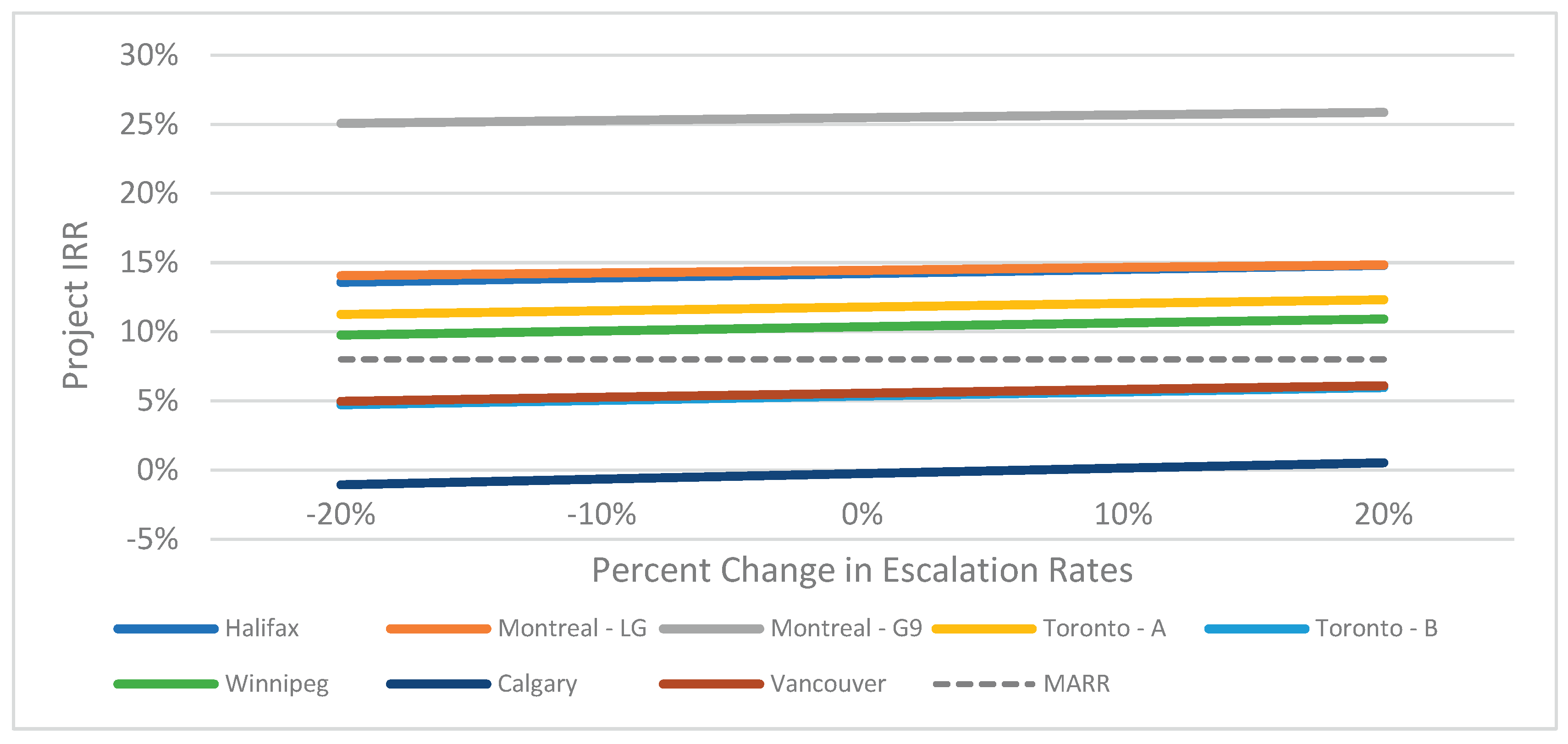
3.6. Escalation Rates
A sensitivity analysis was performed on the utility escalation rates. Since this project is considered over a 25-year span, the returns towards the end of the term will be highly influenced by the escalation rates used.
The expected escalation rates were adjusted by ±10% and ±20%, maintaining eight WET HXs. The escalation rates used in this analysis are shown in Figure 18.
A 20% increase in escalation rates increased returns between 0.40% and 0.78%, with an average of 0.56%. A 20% decrease in escalation rates decreased returns between -0.39% and -0.80%, with an average of -0.56%.
4. Conclusions
The study evaluates the techno-economic feasibility of deploying WET systems in a cold climate, using the TMU campus as a case study. Energy models for each building were simulated with weather data from six major Canadian cities. The annual energy consumption, operating costs, and GHG emissions of conventional HVAC systems were assessed based on local rates and emissions factors. The WET system was compared to these baseline results. A financial model was created to analyze the project's equity returns, and the WET system was optimized for each city to maximize environmental benefits while ensuring sufficient financial returns.
In all cities except Calgary, the WET system achieved an IRR of over 8%. Year 1 gross margins ranged from $128,544 in Calgary to $2,057,855 in Montreal, averaging $852,196. Over 25 years, net cash flows varied from $2,451,672 in Calgary to $40,619,735 in Montreal, with an average of $18,010,632. Calgary had net equity cash flows of $454,121, while Montreal reached $14,503,521, averaging $6,522,071. Winnipeg led in GHG reductions at 5,464 tonnes annually, compared to 21 tonnes in Montreal and a city average of 2,235 tonnes. The sensitivity analysis indicated that supplying only heating or cooling isn’t economically viable, except for heating alone. Reducing the WET system size improved returns by up to 5.84% while increasing heat exchangers (HXs) to 14 decreased returns. Changes in sewer and wastewater temperature affected IRRs slightly. A 20% increase in capital costs decreased returns, while a reduction led to an average increase of 3.05%. A rise in carbon pricing raised project IRRs, with an additional $50 per tonne increase yielding significant boosts.
4.1. Extension of the Current Study
Further multi-objective optimizations could be conducted on the sizes of WET systems to enhance both financial returns and environmental benefits. Investigations could be undertaken at the municipal level to identify optimal locations for installations throughout a sewer network, thereby maximizing energy recovery while mitigating impacts on Wastewater Treatment Plants. The consideration of additional building types would be beneficial. Large structures with substantial energy consumption, such as hospitals, commercial facilities, residential complexes, and community centers with athletic facilities, would be particularly advantageous. The scope of the analysis could be expanded to warmer regions. Furthermore, the operations of the WET system could be optimized to reduce the energy consumption of wastewater pumps while maintaining high COP for the heat pumps.
Data Availability Statement
Data is confidential and will be made available on request.
Acknowledgments
The authors would like to thank Noventa Energy Partners, Mitacs, the TMU Faculty of Engineering and Architectural Science, and Canada First Research Excellence Fund (CFREF) Volt-Age for providing financial support for this research. The authors would also like to thank Dennis Fotinos and Stephen Condie at Noventa Energy Partners for their technical support in successfully completing this study.
Conflicts of Interest
The authors declare that they have no known competing financial interests or personal relationships that could have appeared to influence the work reported in this paper.
Abbreviations
BTU British thermal unit; CDD Cooling Degree Day; COP Coefficient of Performance; DSCR Debt service coverage ratio; GHG Greenhouse Gas; HDD Heating Degree Day; HVAC Heating Ventilation and Air Conditioning; IRR Internal rate of return; MARR Minimum acceptable rate of return; MWh megawatt hour; WET Wastewater Energy Transfer; WET HX Wastewater Heat Exchanger
References
- Government of Canada, Electricity in Canada. 12 Dec 2024. Available online: https://natural-resources.canada.ca/energy/electricity-infrastructure/electricity-canada/7305.
- Canada – Countries & Regions, IEA. 12 Dec 2024. Available online: https://www.iea.org/countries/canada.
- Corbett, M.; Rhodes, E.; Pardy, A.; Long, Z. Pumping up adoption: The role of policy awareness in explaining willingness to adopt heat pumps in Canada. Energy Research and Social Science 2023, 96, 102926. [Google Scholar] [CrossRef]
- Amirirad; Kumar, R.; Fung, A. S.; Leong, W. H. Experimental and simulation studies on air source heat pump water heater for year-round applications in Canada. Energy and Buildings 2018, 165, 141–149. [Google Scholar] [CrossRef]
- Sanongboon, P.; Pettigrew, T. Hybrid energy system optimization model: Electrification of Ontario's residential space and water heating case study. Energy and Climate Change 2022, 3, 100070. [Google Scholar] [CrossRef]
- Postrioti, L.; Baldinelli, G.; Bianchi, F.; Buitoni, G.; Maria, F. D.; Asdrubali, F. An experimental setup for the analysis of an energy recovery system from wastewater for heat pumps in civil buildings. Applied Thermal Engineering 2016, 102, 961–971. [Google Scholar] [CrossRef]
- Seybold, C.; Brunk, M. In-house waste water heat recovery, Federation of European Heating, Ventilation and Air Conditioning Associations, REHVA Journal (2013) 18-2. 12 Dec 2024. Available online: https://www.rehva.eu/rehva-journal/chapter/in-house-waste-water-heat-recovery.
- Hepbasili; Biyik, E.; Ekran, O.; Gunerhan, H.; Araz, M. A key review of wastewater source heat pump (WWSHP) systems. Energy Conversion and Management 2014, 88, 700–722. [Google Scholar] [CrossRef]
- Tomislon, J. Heat Recovery from Wastewater Using a Gravity-Film Heat Exchanger. Federal Energy Management Program; Department of Energy: Washington, DC, USA, 2005. 12 Dec 2024. Available online: https://www.govinfo.gov/content/pkg/GOVPUB-E-PURL-LPS99193/pdf/GOVPUB-E-PURL-LPS99193.pdf.
- City of Toronto, City of Toronto average water consumption. 12 Dec 2024. Available online: https://www.toronto.ca/home/311-toronto-at-your-service/find-service-information/article/?kb=kA06g000001cvc2CAA&searchTerm=Water%20consumption.
- Statistics Canada, World Water Day...by the numbers. 12 Dec 2024. Available online: https://www.statcan.gc.ca/o1/en/plus/5814-world-water-day-eh.
- Veolia. CSR Performance Digest 2014. Available online: https://www.veolia.com/sites/g/files/dvc4206/files/document/2018/12/CSR-2014-EN_0.pdf (accessed on 13 Dec 2024).
- Alisawi, H. A. O. Performance of wastewater treatment during variable temperature. Applied Water Science 2020, 10, 89. [Google Scholar] [CrossRef]
- Huber Technology, Wastewater heat utilisation and reuse of process heat at Munich university hospital, 2020. Available online: https://www.huber.de/huber-report/ablage-berichte/energy-from-wastewater/wastewater-heat-utilisation-and-reuse-of-process-heat-at-munich-university-hospital-klinikum-rechts-der-isar.html?popup=1 (accessed on 13 Dec 2024).
- B Cross, Abundant raw sewage touted to heat and cool aquatic centre, Windsor Star. 1 October 2019. Available online: https://windsorstar.com/news/local-news/abundant-raw-sewage-touted-to-heat-and-cool-aquatic-centre (accessed on 01 Oct 2019).
- Garon, J. Le système d’échange de chaleur pour eaux noires du Faubourg du Moulin. Voir Vert. 19 November 2018. Available online: https://www.voirvert.ca/projets/efficacite-energetique/le-systeme-echange-chaleur-pour-eaux-noires-du-faubourg-du-moulin. (accessed on 01 Oct 2019).
- US Green Building Council. Pathway to Net Zero Energy USGBC Case Study: AGU Headquarters Renovations, US Green Building Council, 2018. Available online: https://insulation.org/io/articles/pathway-to-net-zero-energy-2/ (accessed on 01 Oct 2019).
- European Commission. Study on Energy Prices, Costs and Subsidies and their Impact on Industry and Households, November 2018. Available online: https://op.europa.eu/en/publication-detail/-/publication/d7c9d93b-1879-11e9-8d04-01aa75ed71a1/language-en. (accessed on 01 Oct 2019).
- Sohail, U.; Kwiatek, C.; Fung, A.S.; Joksimovic, D. Techno-Economic Feasibility of Wastewater Heat Recovery for A Large Hospital in Toronto, Canada, August 2019. Published in Proceedings, 15 August 2019. [Google Scholar]
- Available online: https://www.semanticscholar.org/reader/1ac137d203e2991290391e60f790244cab82633c (accessed on 15 Dec 2024).
- Huber Technology, HUBER ThermWin utilizes wastewater heat. Available online: https://www.huber.de/huber-report/ablage-berichte/energy-from-wastewater/huber-thermwin-utilizes-wastewater-heat.html (accessed on 01 Oct 2019).
- Huber Technology, HUBER Pumping Stations Screen ROTAMAT RoK4. Available online: https://www.huber-technology.com/produkte/rechen-fein-und-feinstsiebe/rotamatr-anlagen/huber-schachtsiebanlage-rotamatr-rok4.html (accessed on 01 Oct 2019).
- Rahman, Z.; Selim, M. M.; Fung, A. S.; Taherian, H.; Hossain, M. Energy Audit and Base Case Simulation of Ryerson University Buildings. ASHRAE Transactions 2015, 121, 84–98. [Google Scholar]
- Kwiatek, C.; Sohail, U.; Fung, A.S.; Joksimovic, D. Techno-Economic Feasibility of Sewage Wastewater Heat Recovery (WWHR) Based Community Energy Network (CEN) in a Cold Climate - A Case Study of Ryerson University, Toronto, Canada. IOP Conf. Ser.: Mater. Sci. Eng. 2019, 609, 062028. [Google Scholar] [CrossRef]
- Carier HAP Software. Available online: https://www.carrier.com/commercial/en/us/software/hvac-system-design/hourly-analysis-program/ (accessed on 01 Oct 2019).
- Government of Canada. Engineering Climate Datasets. 2019. Available online: https://climate.weather.gc.ca/prods_servs/engineering_e.html (accessed on 01 Oct 2019).
- Hydro Quebec, 2020 Comparison of Electricity Prices in Major North American Cities," 2020. Available online: https://www.hydroquebec.com/data/documents-donnees/pdf/comparison-electricity-prices.pdf (accessed on 01 Oct 2019).
- Heritage Gas, Historic Rates, 2019. Available online: https://www.heritagegas.com/historic-rates/ (accessed on 01 Oct 2019).
- Ontario Energy Report, Oil and Natural Gas Data Fourth Quater 2019. Available online: https://www.ontarioenergyreport.ca/oil-and-natural-gas.php (accessed on 01 Oct 2019).
- Manitoba Hydro. Wondering about your energy options for space heating? Available online: https://www.hydro.mb.ca/your_home/heating_and_cooling/space_heating_costs.pdf (accessed on 01 Oct 2019).
- Utilities Consumer Advocate, Direct Energy Regulated Services DERS Regulated Gas Rate December 2019. Available online: https://www.ucahelps.alberta.ca/regulated-rates.aspx (accessed on 15 Dec 2024).
- Government of Canada, E-Tables Electricity Canada Provinces and Territories. Available online: https://www.cer-rec.gc.ca/en/data-analysis/energy-markets/provincial-territorial-energy-profiles/provincial-territorial-energy-profiles-canada.html (accessed on 15 Dec 2024).
- Çengel, Y. A.; Ghajar, A. J. Heat and Mass Transfer: Fundamentals & Applications, Published, 6th ed; McGraw Hill Education, 2015. [Google Scholar]
Figure 1.
Typical Average Daily Sewer Water Temperature and Flow Rate Profiles in Toronto, Canada [19].
Figure 1.
Typical Average Daily Sewer Water Temperature and Flow Rate Profiles in Toronto, Canada [19].
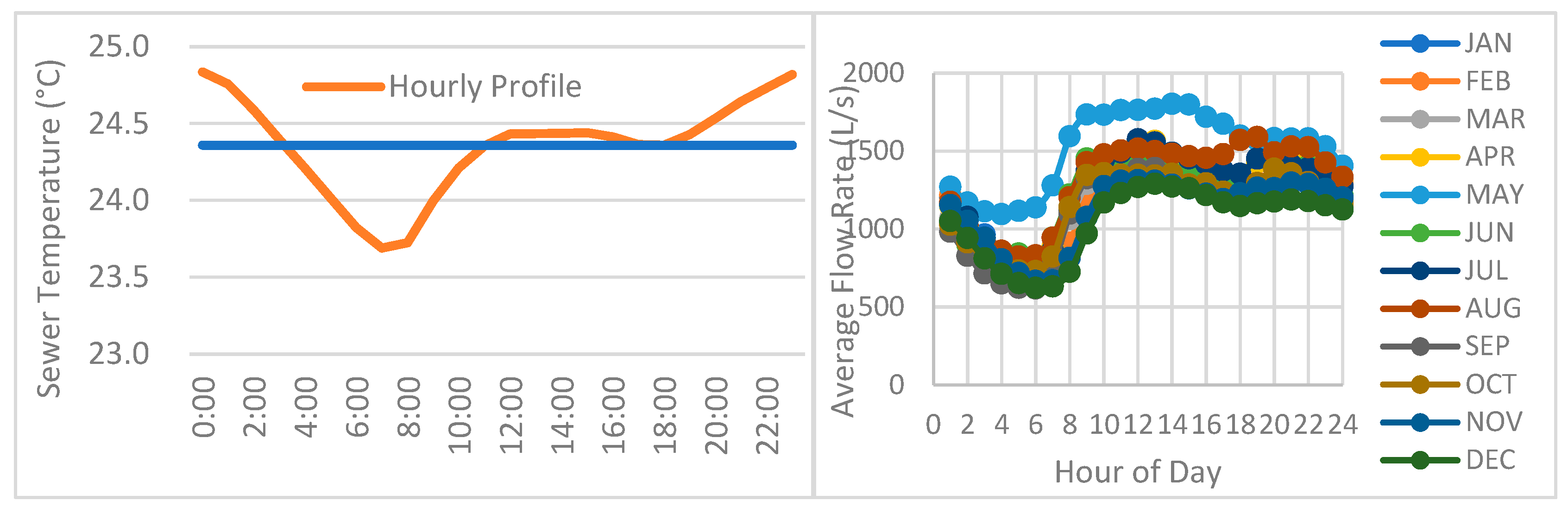
Figure 2.
Proposed WET System Configuration and Cleaning Screen and Built-in Auger Assembly.
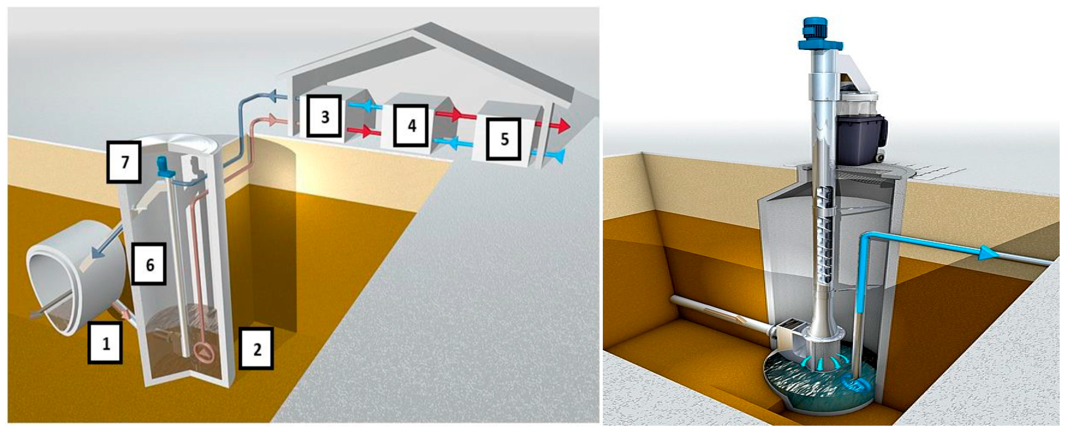
Figure 3.
Analysis Flow Chart.
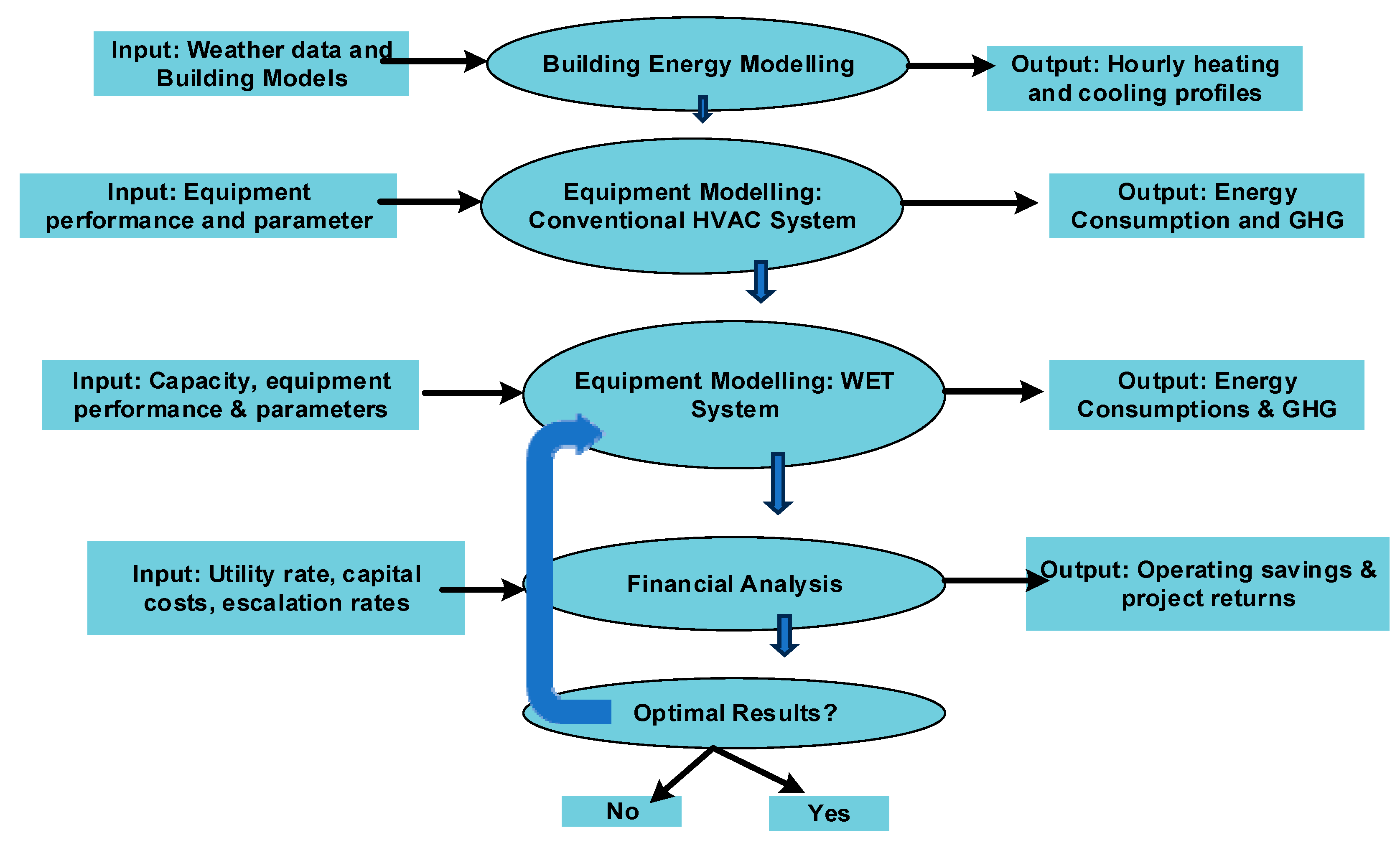
Figure 4.
HDD and CDD vs. Annual Heating and Cooling Energy Demands.
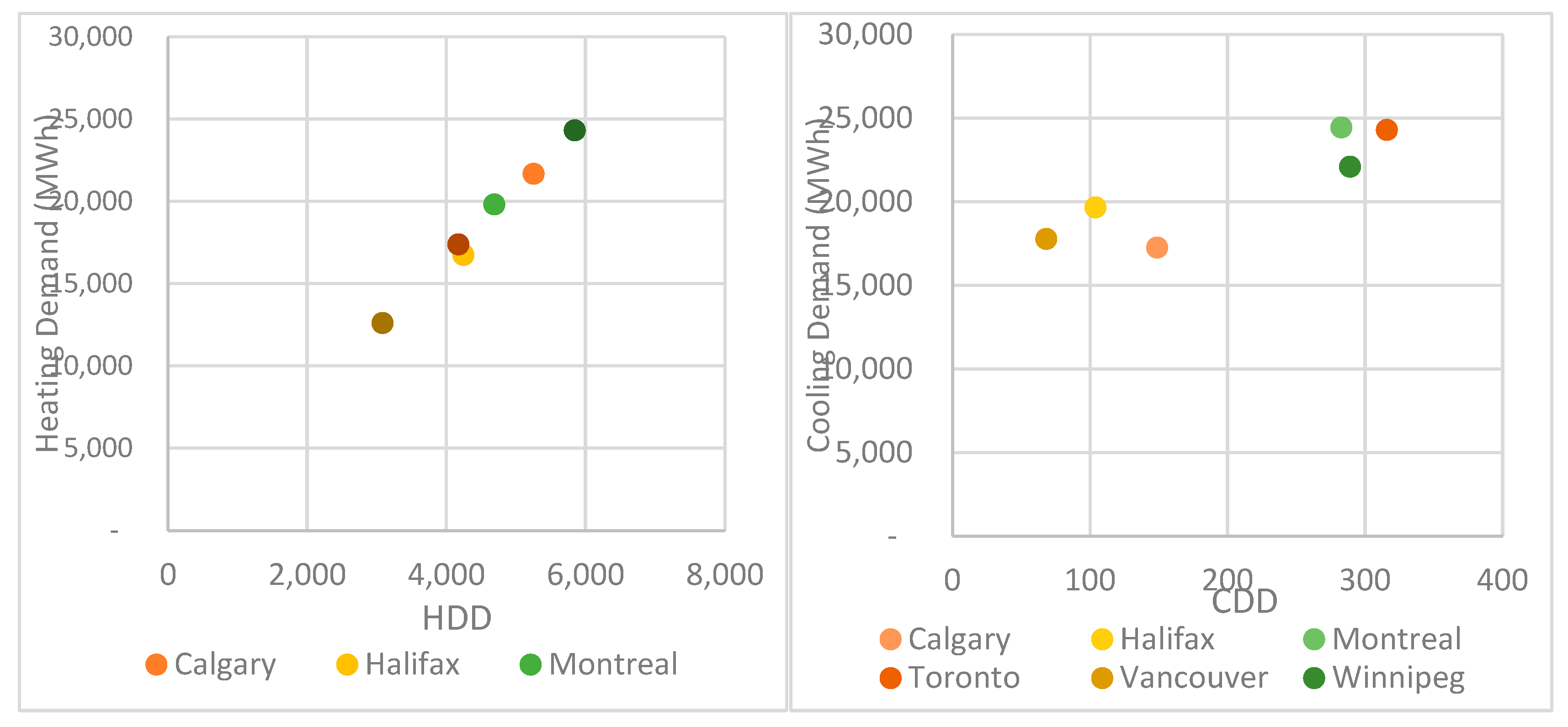
Figure 5.
Representation of the Flow in a Typical Shell-and-Tube HX [32].
Figure 5.
Representation of the Flow in a Typical Shell-and-Tube HX [32].
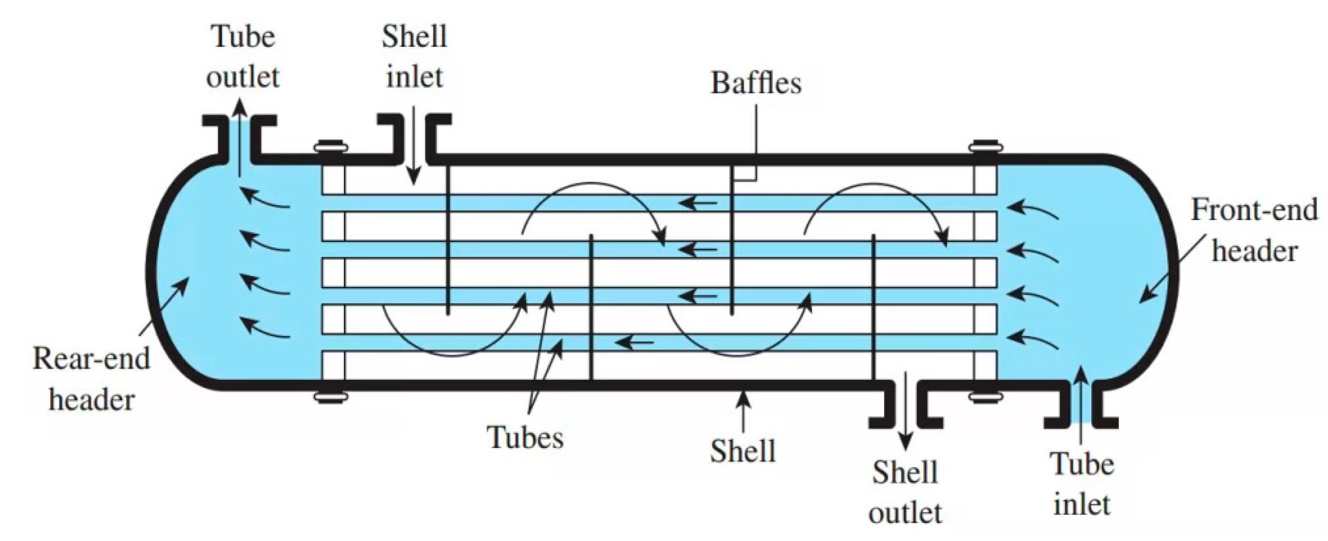
Figure 6.
Wastewater Heat Exchanger Effectiveness vs. Tube Side Flowrate.
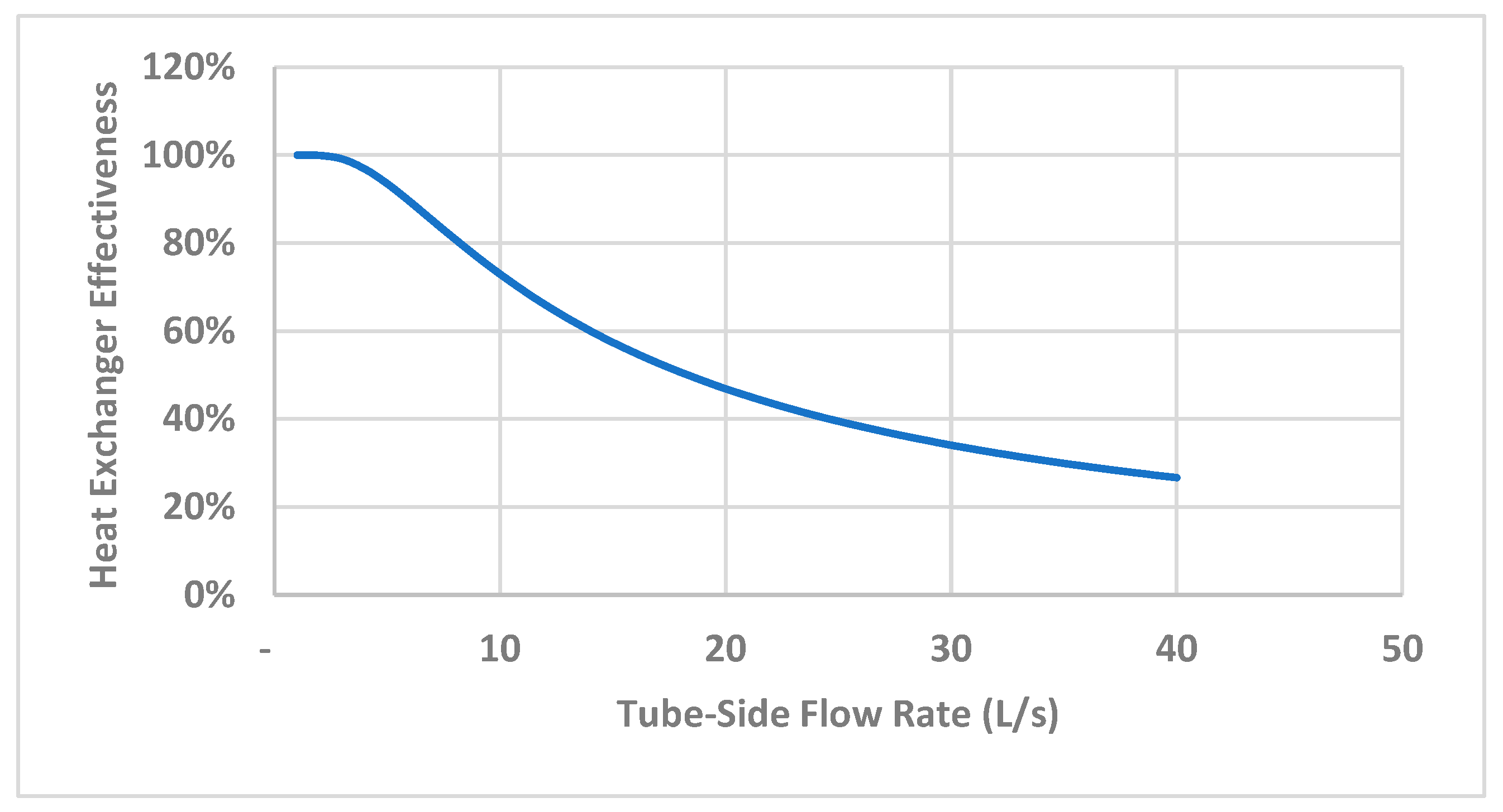
Figure 7.
Hourly Heating Breakdown for the Initial WET-Hybrid System with Eight WET HXs for Toronto.
Figure 7.
Hourly Heating Breakdown for the Initial WET-Hybrid System with Eight WET HXs for Toronto.
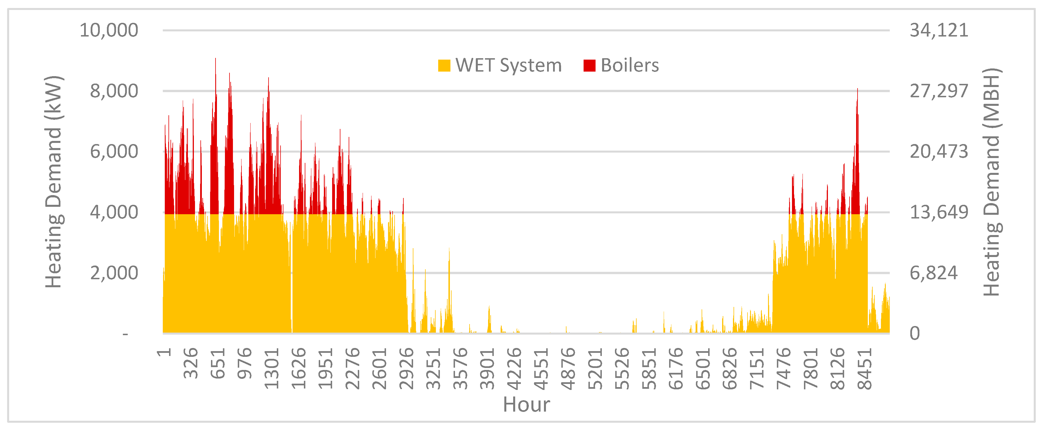
Figure 8.
Hourly Cooling Breakdown for the Initial WET-Hybrid System with Eight WET HXs for Toronto.
Figure 8.
Hourly Cooling Breakdown for the Initial WET-Hybrid System with Eight WET HXs for Toronto.
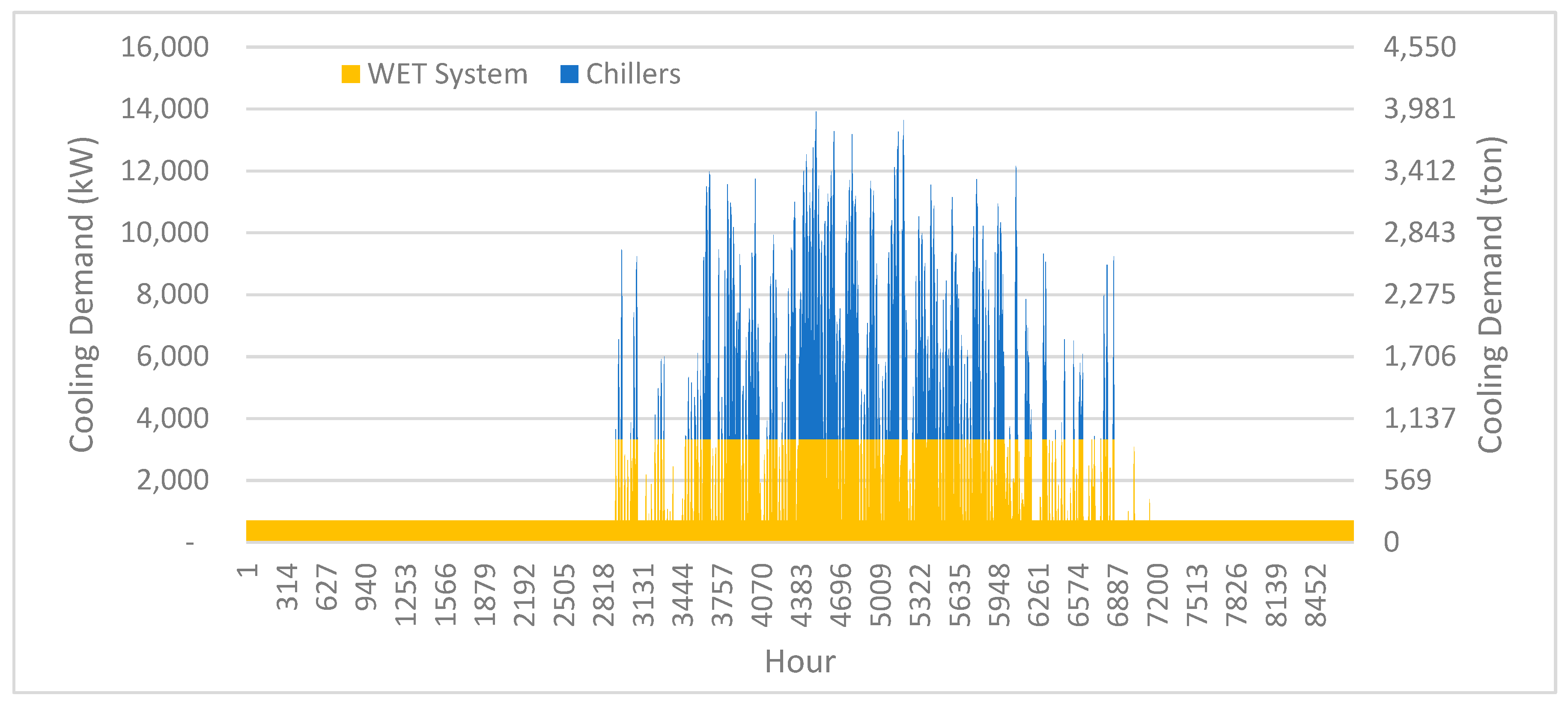
Figure 9.
Total Operating Costs of Conventional and WET-Hybrid Systems and with Costs Reduction.
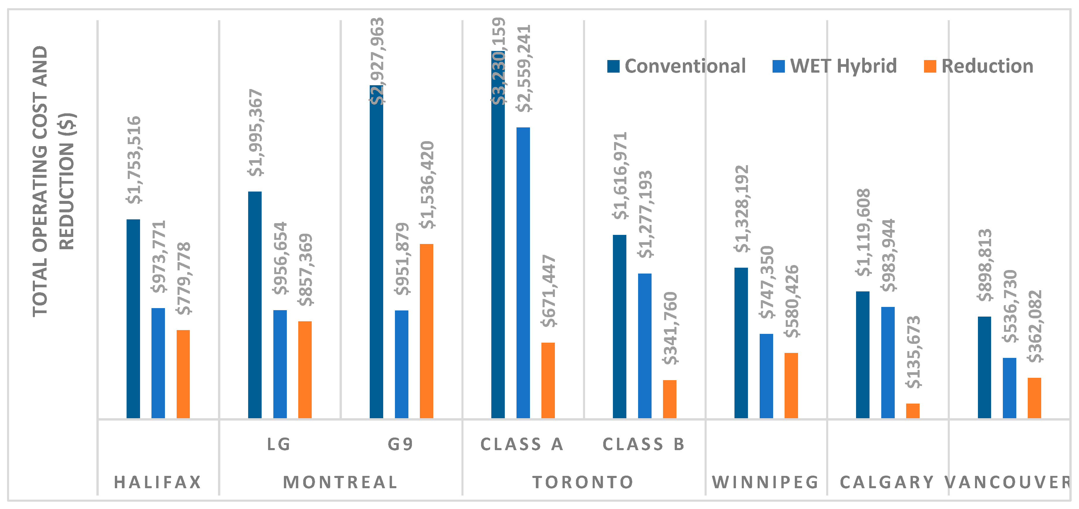
Figure 10.
Total GHG Emissions of Conventional and WET-Hybrid Systems and with GHG Reduction.
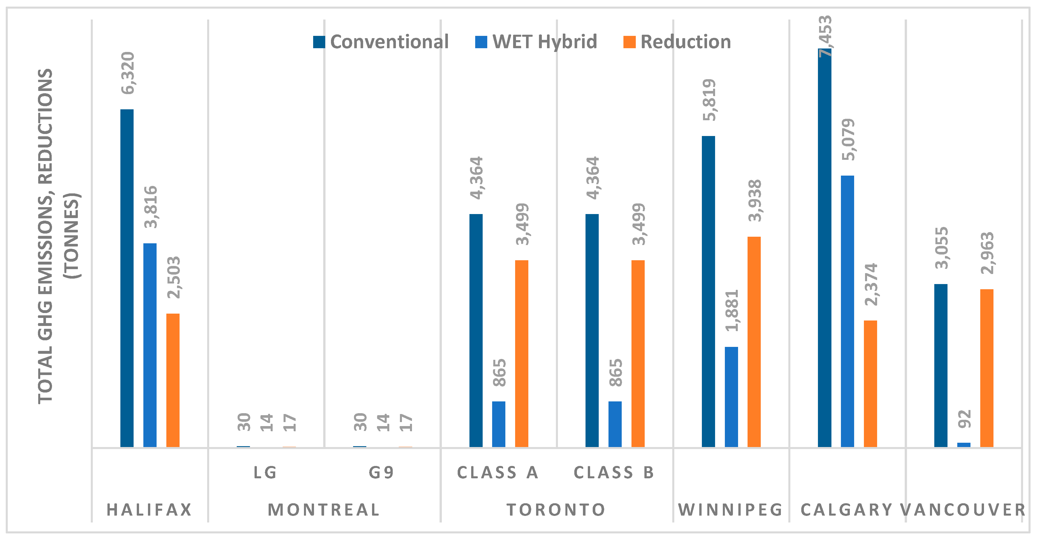
Figure 11.
Comparison of Energy Costs of the Optimal WET-Hybrid and Conventional Systems.
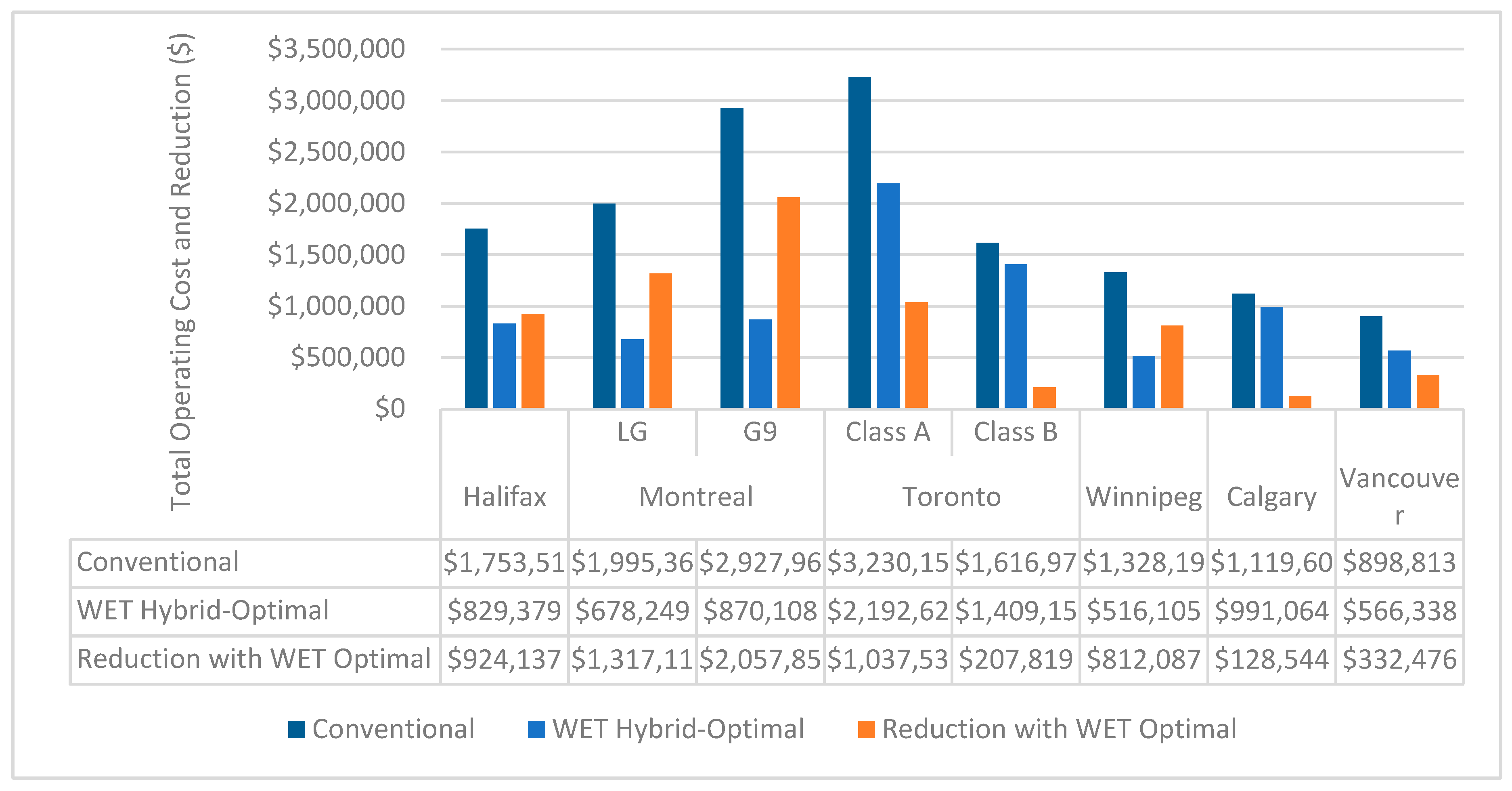
Figure 12.
Comparison of GHG Emissions of the Optimal WET-Hybrid and Conventional Systems.
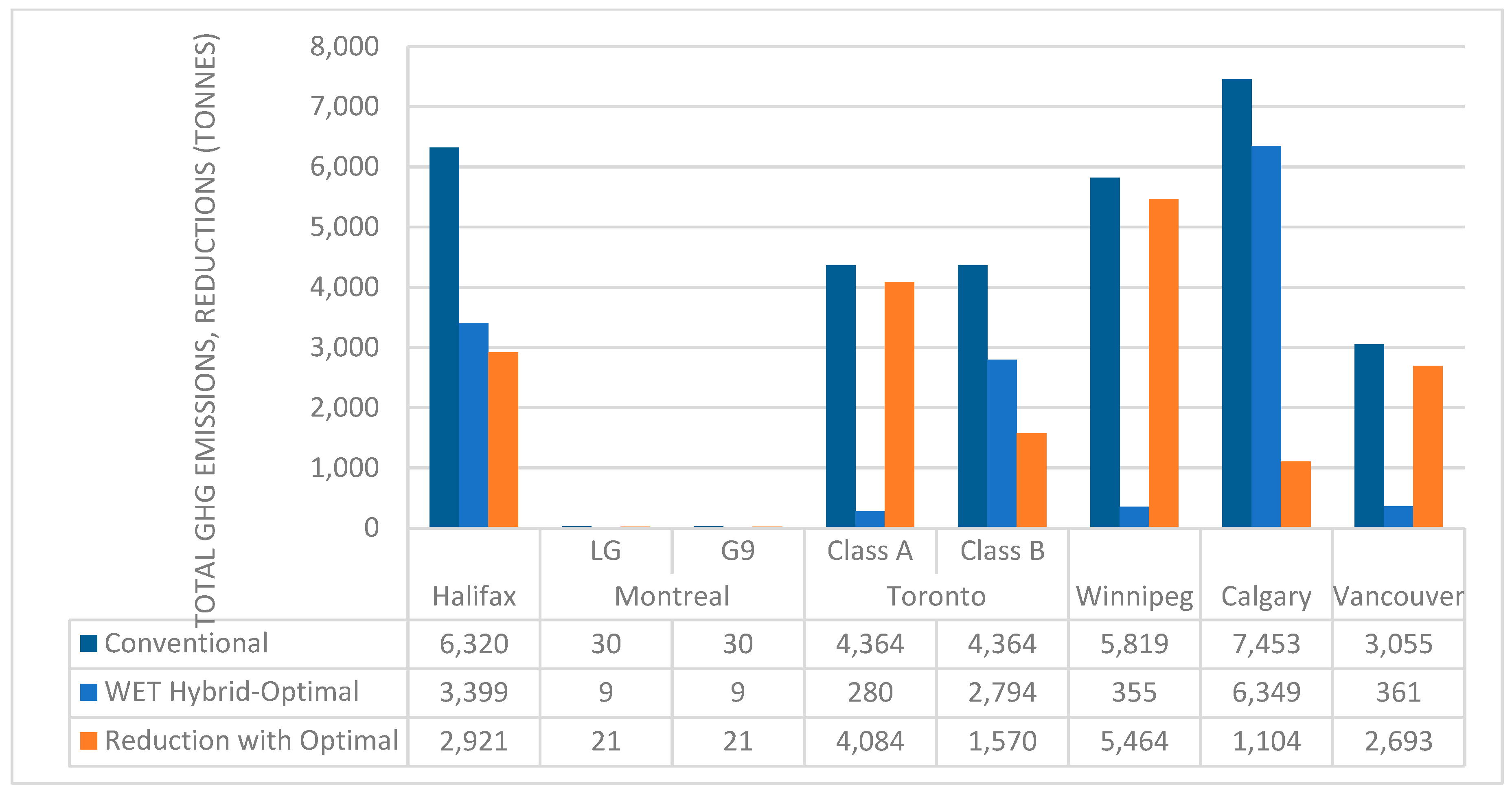
Figure 13.
Breakdown of GHG Emissions for the Conventional Base Case and the Optimal WET Systems.
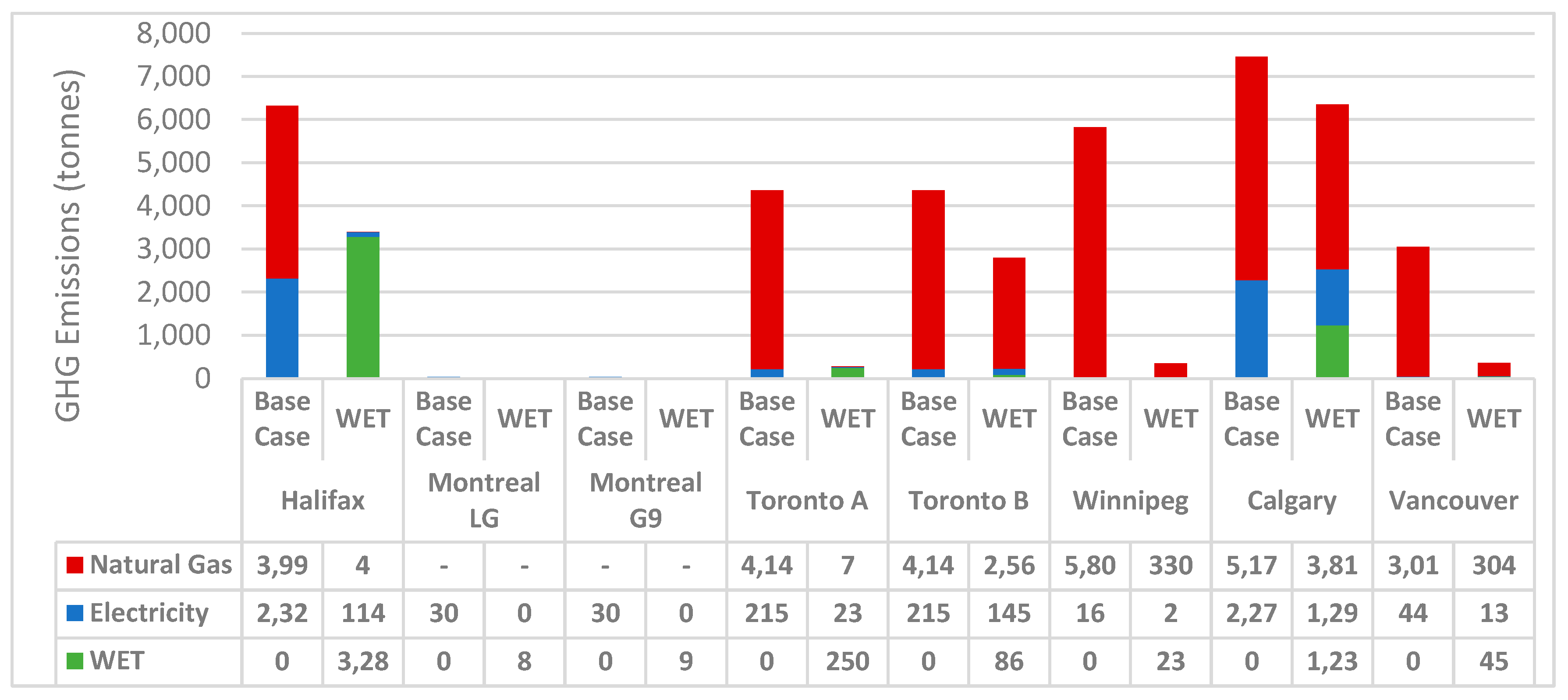
Figure 14.
WET System Size Sensitivity.
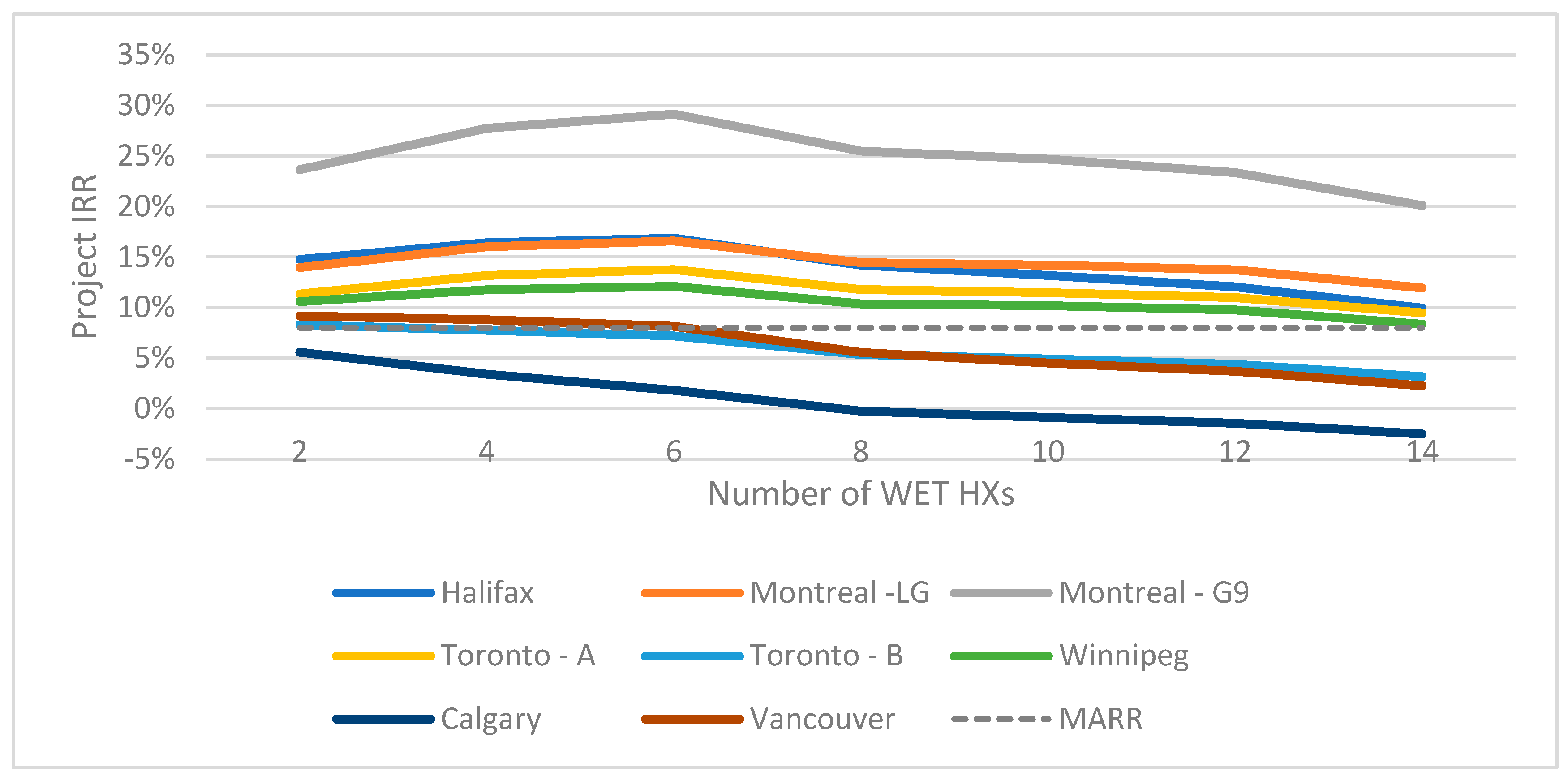
Figure 15.
Sewer Temperature Sensitivity.
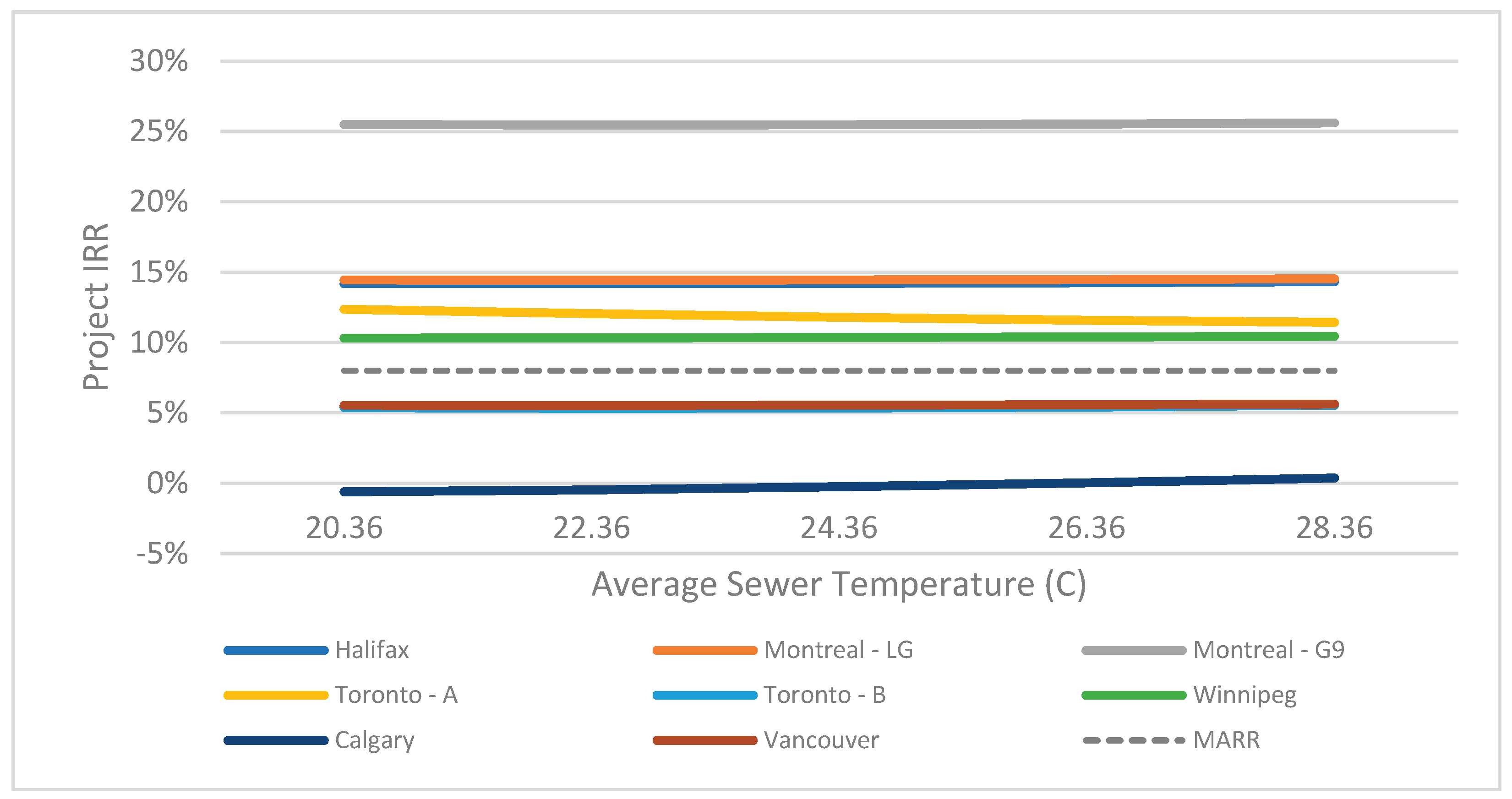
Figure 16.
Capital Cost Sensitivity.
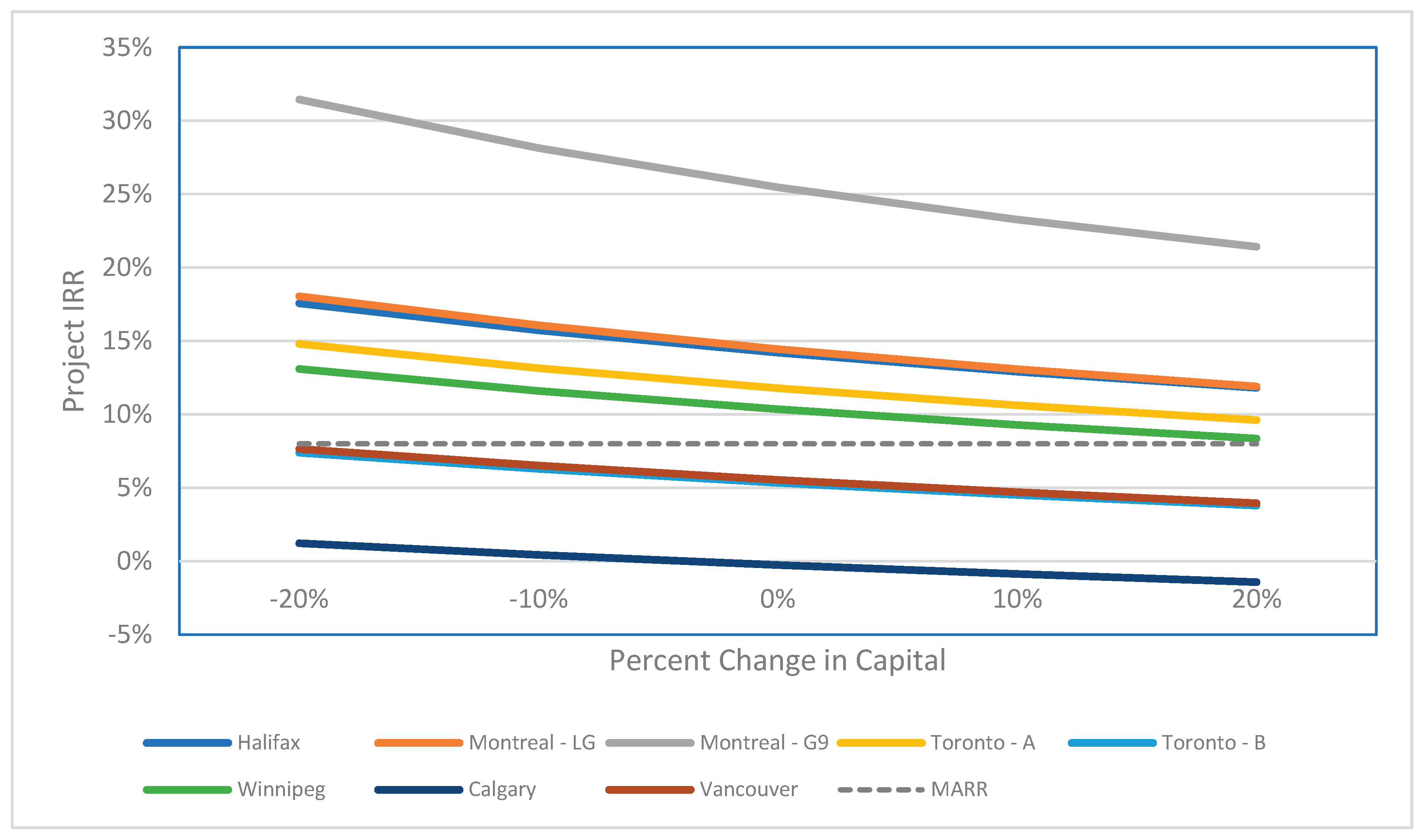
Figure 17.
Additional Carbon Price Sensitivity.
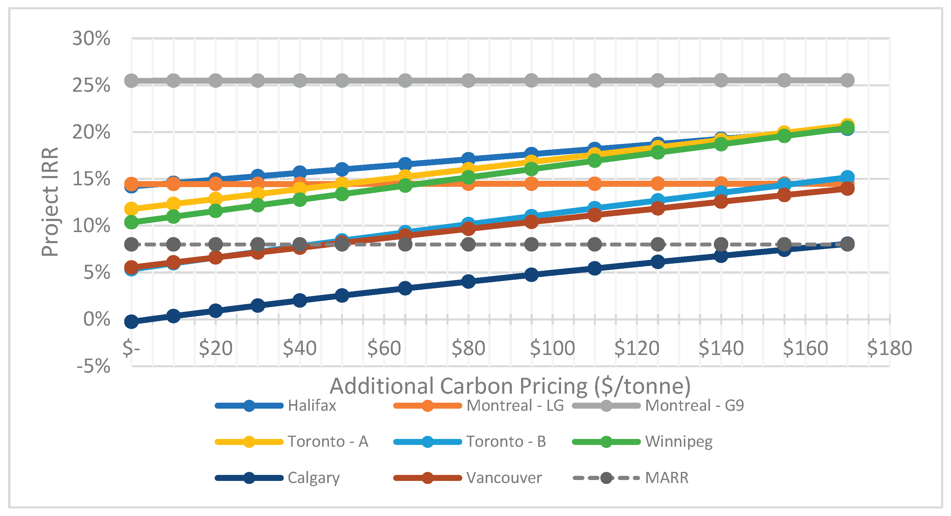
Figure 18.
Utility Escalation Rate Sensitivity.

| Cost | GHG Emissions | |||||||
|---|---|---|---|---|---|---|---|---|
| Electricity | Natural Gas | Electricity-Natural Gas | Electricity | Natural Gas | Electricity- Natural Gas | |||
| City | $/kWh | $/m3 | $/kWhe | Cost Ratio | g/kWh | g/m3 | g/kWhe | GHG Ratio |
| Halifax, Nova Scotia | $0.1689 | $0.384 | $0.0364 | 4.64 | 600.0 | 1890 | 179.0 | 3.35 |
| Montreal, Quebec | $0.0730 | - | - | - | 1.2 | 1890 | 179.0 | 0.01 |
| Toronto, Ontario | $0.1110 | $0.265 | $0.0251 | 4.42 | 40.0 | 1890 | 179.0 | 0.22 |
| Winnipeg, Manitoba | $0.0960 | $0.288 | $0.0273 | 3.52 | 3.4 | 1890 | 179.0 | 0.02 |
| Calgary, Alberta | $0.1483 | $0.182 | $0.0172 | 8.60 | 790.0 | 1890 | 179.0 | 4.41 |
| Vancouver, British Columbia | $0.1151 | $0.185 | $0.0175 | 6.57 | 12.9 | 1890 | 179.0 | 0.07 |
Table 2.
Summary of Heating and Cooling Demands for Modelled Buildings in Selected Cities.
| Halifax, NS | Montreal, QC | Toronto, ON | Winnipeg, MN | Calgary, AB | Vancouver, BC | ||
|---|---|---|---|---|---|---|---|
| Annual Heating | MWh | 16,743 | 19,812 | 17,381 | 24,313 | 21,671 | 12,610 |
| MMBtu | 57,132 | 67,604 | 59,307 | 82,959 | 73,946 | 43,028 | |
| Heating Peak | MW | 9.87 | 10.02 | 9.09 | 11.45 | 10.23 | 7.03 |
| MBH | 33,687 | 34,193 | 31,028 | 39,066 | 34,898 | 23,979 | |
| HDD | (°C-days) | 4,246 | 4,689 | 4,174 | 5,846 | 5,256 | 3,084 |
| Annual Cooling | MWh | 19,647 | 24,425 | 24,283 | 22,088 | 17,252 | 17,765 |
| MMBtu | 67,039 | 83,344 | 82,857 | 75,369 | 58,868 | 60,616 | |
| Cooling Peak | MW | 12.57 | 16.33 | 13.92 | 16.51 | 10.47 | 10.63 |
| tons | 3,574 | 4,643 | 3,958 | 4,696 | 2,976 | 3,022 | |
| CDD | (°C-days) | 104 | 283 | 316 | 289 | 149 | 68 |
Table 3.
Conventional HVAC System Utility Consumption, Operating Cost and GHG Emissions.
| Halifax | Montreal | Toronto | Winnipeg | Calgary | Vancouver | ||||
|---|---|---|---|---|---|---|---|---|---|
| LG | G9 | Class A | Class B | ||||||
| Electricity | |||||||||
| Electricity Consumption | kWh | 3,871,788 | 25,231,639 | 25,231,639 | 5,372,027 | 5,372,027 | 4,559,797 | 2,885,332 | 3,448,288 |
| Electricity Cost | $ | $618,373 | $1,933,343 | $2,865,938 | $2,554,762 | $941,894 | $317,222 | $32,698 | $401,214 |
| Natural Gas | |||||||||
| Natural Gas Consumption | m3 | 2,114,755 | - | - | 2,195,263 | 2,195,263 | 3,070,766 | 2,737,130 | 1,592,689 |
| Natural Gas Cost | $ | $1,039,936 | - | - | $497,939 | $497,619 | $849,394 | $497,122 | $293,149 |
| Water | |||||||||
| Water Consumption | m3 | 50,750 | 68,916 | 68,916 | 68,253 | 68,253 | 59,403 | 40,628 | 44,802 |
| Water Cost | $ | $49,532 | - | - | $116,030 | $116,030 | $108,113 | $53,223 | $164,128 |
| Chemicals | |||||||||
| Chemical Cost | $ | $45,675 | $62,025 | $62,025 | $61,428 | $61,428 | $53,463 | $36,565 | $40,322 |
| Total Operating Expenses | $ | $1,753,516 | $1,995,367 | $2,927,963 | $3,230,159 | $1,616,971 | $1,328,192 | $1,119,608 | $898,813 |
| GHG Emissions | tonnes | 6,320 | 30 | 30 | 4,364 | 4,364 | 5,819 | 7,453 | 3,055 |
Table 4.
WET System Capital Cost Breakdown [31].
Table 4.
WET System Capital Cost Breakdown [31].
| Major Equipment | # of Units | Cost Per Unit | Total | ||||
|---|---|---|---|---|---|---|---|
| WET Heat Exchanger | 8 | $ | 250,000 | $ | 2,000,000 | ||
| Wastewater Screen Assembly | 2 | $ | 130,000 | $ | 260,000 | ||
| Wastewater Supply Pumps | 32.6 L/s x 8 WET HXs | $ | 184.05/(L/s) | $ | 48,000 | ||
| Hot Water Supply Pumps | 16 L/s x 8 WET HXs | $ | 156.25/(L/s) | $ | 20,000 | ||
| Chilled Water Supply Pumps | 16 L/s x 8 WET HXs | $ | 156.25/(L/s) | $ | 20,000 | ||
| Heat Pump | 140 tons x 8 WET HXs | $ | 678.57/ton | $ | 760,000 | ||
| Major Equipment Sub-Total | $ | 3,108,000 | |||||
| Construction | Initial Cost | # of Units | Incremental Cost | Total | |||
| Sewer Interconnect | $ | 125,000 | $ | 125,000 | |||
| Wetwell | 2 Screen Assemblies | $ | 425,000 | $ | 850,000 | ||
| Intermediary Piping | $ | 150,000 | 8 | $ | 20,000 | $ | 310,000 |
| Balance of Plant | 25% | $ | 4,393,000 | $ | 1,098,250 | ||
| Construction Sub-Total | $ | 2,383,250 | |||||
| Design/Permits | # of Units | % Rate | Total | ||||
| Civil Design | 12 % | $ | 1,160,000 | $ | 139,200 | ||
| Mechanical Design | 10 % | $ | 4,206,250 | $ | 420,625 | ||
| Electrical Design | 5 % | $ | 3,108,000 | $ | 155,400 | ||
| Controls Design | 3 % | $ | 3,108,000 | $ | 93,240 | ||
| Sewer Access Permit | 2 | $ | 25,000 | $ | 50,000 | ||
| Design/Permits Sub-Total | $ | 858,465 | |||||
| Total Project Capital Cost | Total | ||||||
| Total Project Capital Cost | $ | 6,349,715 | |||||
| Contingency | % Rate | Total | |||||
| Contingency | 5 % | $ | 3,241,715 | $ | 162,086 | ||
| Total Project Cost | $ | 6,511,801 | |||||
Table 5.
Utility Rate Escalation [31] and Debt Loan Parameters.
Table 5.
Utility Rate Escalation [31] and Debt Loan Parameters.
| Utility Rate Escalation | Debt loan parameters | ||
|---|---|---|---|
| Commodity | Escalation Rate | Parameter | Value |
| Electricity | 2.0 % | Debt Term | 25 years |
| Natural Gas | 3.0 % | Interest Rate | 3 % |
| Water | 2.5 % | Borrowed Portion of Capital | 70 % |
| Cooling Tower Chemicals | 2.5 % | Minimum Required Debt Service Coverage Ratio (DSCR) | 1.3 |
Table 6.
Relations used for financial analysis [24].
Table 6.
Relations used for financial analysis [24].
| Equation for Financial Analysis |
|---|
Table 7.
Financial Results for the Initial WET-Hybrid Case with 8 HXs.
| Halifax | Montreal | Toronto | Winnipeg | Calgary | Vancouver | |||
|---|---|---|---|---|---|---|---|---|
| LG | G9 | Class A | Class B | |||||
| Year 1 Operations | ||||||||
| Year 1 Conventional HVAC Operating Cost | $1,753,549 | $1,814,023 | $2,488,298 | $3,230,688 | $1,618,954 | $1,327,777 | $1,119,616 | $898,812 |
| Year 1 Optimized Hybrid WET Operating Cost | $973,771 | $956,654 | $951,879 | $2,559,241 | $1,277,193 | $747,350 | $983,944 | $536,730 |
| Year 1 Operating Savings | $779,778 | $857,369 | $1,536,420 | $671,447 | $341,760 | $580,426 | $135,673 | $362,082 |
| Project Returns | ||||||||
| Capital Investment | $6,511,801 | $6,511,801 | $6,511,801 | $6,511,801 | $6,511,801 | $6,511,801 | $6,511,801 | $6,511,801 |
| 25 Year Savings | $29,042,294 | $27,542,623 | $49,292,816 | $23,600,119 | $13,040,159 | $21,275,673 | $6,254,825 | $13,219,725 |
| 25 Year Net Cashflow | $22,530,493 | $21,030,823 | $42,781,015 | $17,088,318 | $6,528,358 | $14,763,872 | $(256,976) | $6,707,924 |
| Project IRR | 14.20% | 14.44% | 25.47% | 11.78% | 5.34% | 10.35% | -0.26% | 5.54% |
| Debt Financing | ||||||||
| % of Capital as Debt | 70.00% | 70.00% | 70.00% | 70.00% | 70.00% | 70.00% | 27.92% | 70.00% |
| Capital as Debt | $4,558,261 | $4,558,261 | $4,558,261 | $4,558,261 | $4,558,261 | $4,558,261 | $1,818,365 | $4,558,261 |
| Year 1 DSCR | 2.98 | 3.28 | 5.87 | 2.57 | 1.31 | 2.22 | 1.30 | 1.38 |
| Equity Returns | ||||||||
| Capital Contribution | $1,953,540 | $1,953,540 | $1,953,540 | $1,953,540 | $1,953,540 | $1,953,540 | $4,693,436 | $1,953,540 |
| 25 Year Savings | $13,975,287 | $12,948,013 | $27,846,895 | $10,247,398 | $3,013,825 | $8,655,152 | $1,923,495 | $3,136,828 |
| 25 Year Net Cashflow | $12,021,747 | $10,994,473 | $25,893,355 | $8,293,857 | $1,060,285 | $6,701,612 | $(2,769,941) | $1,183,287 |
| Equity IRR | 20.30% | 21.36% | 45.05% | 15.72% | 2.62% | 12.83% | -4.74% | 2.99% |
Table 8.
WET-Hybrid Supply and Building Demands for the Optimal WET-Hybrid Systems.
| Halifax | Montreal | Toronto | Winnipeg | Calgary | Vancouver | ||||
|---|---|---|---|---|---|---|---|---|---|
| LG | G9 | Class A | Class B | ||||||
| Project IRR | |||||||||
| Project IRR | 8.09% | 8.13% | 8.29% | 8.74% | 8.01% | 8.09% | 5.58% | 8.13% | |
| WET System Size | |||||||||
| Number of WET HXs | 18 | 23 | 36 | 18 | 3 | 15 | 2 | 6 | |
| Heating | |||||||||
| WET Supply | MWh | 16,727 | 19,654 | 19,654 | 17,353 | 6,644 | 22,931 | 5,691 | 11,339 |
| MMBTU | 57,074 | 67,061 | 67,061 | 59,211 | 22,671 | 78,244 | 19,420 | 38,689 | |
| Building Demand | MWh | 16,744 | 19,813 | 19,813 | 17,381 | 17,381 | 24,313 | 21,671 | 12,610 |
| MMBTU | 57,132 | 67,604 | 67,604 | 59,307 | 59,307 | 82,959 | 73,946 | 43,028 | |
| Percent of Annual | % | 99.9% | 99.2% | 99.2% | 99.8% | 38.2% | 94.3% | 26.3% | 89.9% |
| WET Peak | kW | 8,862 | 10,021 | 10,021 | 8,862 | 1,477 | 7,385 | 985 | 2,954 |
| MBH | 30,240 | 34,193 | 34,193 | 30,240 | 5,040 | 25,200 | 3,360 | 10,080 | |
| Building Peak | kW | 9,873 | 10,021 | 10,021 | 9,093 | 9,093 | 11,449 | 10,228 | 7,028 |
| MBH | 33,687 | 34,193 | 34,193 | 31,028 | 31,028 | 39,066 | 34,898 | 23,979 | |
| Percent of Peak | % | 89.8% | 100.0% | 100.0% | 97.5% | 16.2% | 64.5% | 9.6% | 42.0% |
| Cooling | |||||||||
| WET Supply | MWh | 14,406 | 19,605 | 20,208 | 18,134 | 7,659 | 15,224 | 6,388 | 9,715 |
| TonHr | 4,096,325 | 5,574,609 | 5,746,093 | 5,156,262 | 2,177,871 | 4,329,006 | 1,816,489 | 2,762,404 | |
| Building Demand | MWh | 15,044 | 20,232 | 20,232 | 20,026 | 20,026 | 17,584 | 12,321 | 13,217 |
| TonHr | 4,277,811 | 5,752,833 | 5,752,833 | 5,694,177 | 5,694,177 | 4,999,916 | 3,503,357 | 3,758,192 | |
| Percent of Annual | % | 95.8% | 96.9% | 99.9% | 90.6% | 38.2% | 86.6% | 51.8% | 73.5% |
| WET Peak | kW | 7,511 | 9,598 | 15,023 | 7,511 | 1,252 | 6,260 | 835 | 2,504 |
| tons | 2,136 | 2,729 | 4,272 | 2,136 | 356 | 1,780 | 237 | 712 | |
| Building Peak | kW | 12,570 | 16,330 | 16,330 | 13,921 | 13,921 | 16,514 | 10,466 | 10,628 |
| tons | 3,574 | 4,643 | 4,643 | 3,958 | 3,958 | 4,696 | 2,976 | 3,022 | |
| Percent of Peak | % | 59.8% | 58.8% | 92.0% | 54.0% | 9.0% | 37.9% | 8.0% | 23.6% |
Table 9.
Financial Results for the Optimal WET-Hybrid System.
| Halifax | Montreal | Toronto | Winnipeg | Calgary | Vancouver | |||
|---|---|---|---|---|---|---|---|---|
| LG | G9 | Class A | Class B | |||||
| Number of WET HXs | ||||||||
| Number of WET HXs | 18 | 23 | 36 | 18 | 3 | 15 | 2 | 6 |
| Year 1 Operations | ||||||||
| Year 1 Conventional Operating Cost | $1,753,516 | $1,995,367 | $2,927,963 | $3,230,159 | $1,616,971 | $1,328,192 | $1,119,608 | $898,813 |
| Year 1 Optimized WET Operating Cost | $829,379 | $678,249 | $870,108 | $2,192,627 | $1,409,151 | $516,105 | $991,064 | $566,338 |
| Year 1 Operating Savings | $924,137 | $1,317,118 | $2,057,855 | $1,037,531 | $207,819 | $812,087 | $128,544 | $332,476 |
| Project Returns | ||||||||
| Capital Investment | $12,906,417 | $16,524,163 | $25,425,778 | $12,906,417 | $2,894,055 | $11,240,295 | $2,338,681 | $4,560,177 |
| 25 Year Savings | $34,391,959 | $42,315,404 | $66,045,513 | $35,773,232 | $7,615,368 | $29,830,606 | $4,790,352 | $12,118,598 |
| 25 Year Net Cashflow | $21,485,542 | $25,791,241 | $40,619,735 | $22,866,815 | $4,721,314 | $18,590,311 | $2,451,672 | $7,558,422 |
| Project IRR | 8.09% | 8.13% | 8.29% | 8.74% | 8.01% | 8.09% | 5.58% | 8.13% |
| Debt Financing | ||||||||
| % of Capital as Debt | 70.00% | 70.00% | 70.00% | 70.00% | 70.00% | 70.00% | 70.00% | 70.00% |
| Capital as Debt | $9,034,492 | $11,566,914 | $17,798,044 | $9,034,492 | $2,025,838 | $7,868,207 | $1,637,076 | $3,192,124 |
| Year 1 DSCR | 1.78 | 1.98 | 2.01 | 2.00 | 1.79 | 1.80 | 1.37 | 1.81 |
| Equity Returns | ||||||||
| Capital Contribution | $3,871,925 | $4,957,249 | $7,627,733 | $3,871,925 | $868,216 | $3,372,089 | $701,604 | $1,368,053 |
| 25 Year Earnings | $11,827,635 | $13,966,966 | $22,131,265 | $12,773,807 | $2,586,073 | $10,217,474 | $1,155,726 | $4,156,420 |
| 25 Year Net Cashflow | $7,955,710 | $9,009,717 | $14,503,532 | $8,901,882 | $1,717,857 | $6,845,386 | $454,121 | $2,788,367 |
| Equity IRR | 8.39% | 8.51% | 8.84% | 9.73% | 8.23% | 8.39% | 3.12% | 8.46% |
Table 10.
WET System IRRs for the Cooling and Heating Sensitivity.
| HVAC Scenario | Halifax | Montreal | Toronto | Winnipeg | Calgary | Vancouver | ||||||||||
|---|---|---|---|---|---|---|---|---|---|---|---|---|---|---|---|---|
| LG | G9 | Class A | Class B | |||||||||||||
|
IRR % |
+/- % |
IRR % |
+/- % |
IRR % |
+/- % |
IRR % |
+/- % |
IRR % |
+/- % |
IRR % |
+/- % |
IRR % |
+/- % |
IRR % |
+/- % |
|
| Cooling and Heating | 14.2 | 0.0 | 14.4 | 0.0 | 25.5 | 0.0 | 11.8 | 0.0 | 5.3 | 0.0 | 10.4 | 0.0 | -0.3 | 0.0 | 5.5 | 0.0 |
| Cooling Only | -2.2 | -16.4 | -5.1 | -19.5 | -3.9 | -29.4 | 4.4 | -7.4 | 0.6 | -4.7 | -2.4 | -12.8 | -3.4 | -3.2 | 1.0 | -4.5 |
| Heating Only | 10.1 | -4.1 | 12.7 | -1.8 | 22.7 | -2.8 | 3.8 | -8.0 | -5.3 | -10.7 | 6.8 | -3.6 | N/A | N/A | -3.6 | -9.1 |
Disclaimer/Publisher’s Note: The statements, opinions and data contained in all publications are solely those of the individual author(s) and contributor(s) and not of MDPI and/or the editor(s). MDPI and/or the editor(s) disclaim responsibility for any injury to people or property resulting from any ideas, methods, instructions or products referred to in the content. |
© 2026 by the authors. Licensee MDPI, Basel, Switzerland. This article is an open access article distributed under the terms and conditions of the Creative Commons Attribution (CC BY) license (http://creativecommons.org/licenses/by/4.0/).
Copyright: This open access article is published under a Creative Commons CC BY 4.0 license, which permit the free download, distribution, and reuse, provided that the author and preprint are cited in any reuse.


