
Submitted:
04 January 2026
Posted:
06 January 2026
You are already at the latest version
Abstract
An up-to-date catalog of resident space objects orbiting Earth is essential for effective space environment management, which requires the orbital propagation of tens of thousands of objects. Although ephemeris data are publicly accessible through catalogs such as NORAD, other organizations generate independent datasets based on their own observations. Due to the large number of objects, orbit propagators have become indispensable tools that must balance accuracy with computational efficiency. High-fidelity numerical propagators provide accurate results at the expense of computational intensity, whereas analytical models, such as SGP4, offer greater efficiency at the expense of neglecting certain dynamical effects. Hybrid orbit propagators have been proposed as an alternative by combining classical propagators to integrate the deterministic motion with machine learning or statistical time-series techniques to predict unmodeled effects and address intrinsic uncertainties. This work presents a hybrid version of the SGP4 propagator, particularly fitted for Galileo-type orbits. HSGP4 employs machine learning techniques and operates with a Hybrid Two-Line Element set (HTLE), which extends the classical TLE by including model parameters. The propagation process integrates standard SGP4 outputs with a forecast of SGP4 error, yielding more accurate ephemerides while maintaining its computational efficiency.
Keywords:
hybrid orbit propagator
; SGP4
; artificial neural network
; Galileo-type orbits
1. Introduction
Maintaining a running catalog of space objects orbiting the Earth is essential for effective management of the near-Earth space environment. Ephemerides information is publicly accessible via the NORAD catalog, while other organizations, such as the European Space Agency (ESA), also provide data derived from their own observations. Sustaining these catalogs over time requires both comprehensive observational data and accurate predictions of object trajectories, which are achieved through orbit-propagation methods.
Orbit propagation refers to computer software that implements a solution to the dynamical systems governing the motion of Resident Space Objects (RSOs). Such software determines the state of an RSO at a specified time, given an initial condition. The accuracy and computational efficiency of an orbit propagator depend primarily on the force model used in the dynamical system and the integration technique employed to obtain the solution.
The primary force considered is the gravitational attraction of an ideally spherical Earth. However, other forces, such as Earth’s nonsphericity, atmospheric drag, gravitational perturbations from other celestial bodies, and solar radiation pressure, can significantly modify the RSO’s trajectory. An important characteristic of this dynamical system is that not all perturbations need to be included in every model; typically, only those most relevant to the specific orbiter, its orbital characteristics, and the mission’s scientific objectives are considered. Integration techniques further categorize orbit propagators into general perturbations, special perturbations, and semianalytic theories.
General perturbation, or analytical, theories [1,2,3,4,5] are derived from direct analytic integration of the equations of motion and are primarily characterized by their ability to preserve the essential qualitative behavior of orbital motion. These approaches are based on truncated series expansions [6,7,8,9,10,11,12,13]. The resulting solutions are valid for arbitrary initial conditions and are formulated as explicit functions of time, physical parameters, and integration constants. Once the RSO state is known at a given time, its future state can be determined through a single evaluation of the analytical solution. The accuracy of a general perturbation theory is directly proportional to the fidelity of its force model and the order of the truncated expansion employed.
On the other hand, special perturbation methods refer [14,15] to the direct numerical integration of the equations of motion, including any external forces. In these approaches, introducing a new force into the equations of motion is achieved by simply expressing the perturbation in terms of time and the object’s state. In addition, achieving high accuracy with these methods requires using small integration steps, which penalises their computational efficiency. Nevertheless, special perturbation theories are usually much slower than their analytical counterparts, though generally provide greater accuracy.
Finally, semianalytical techniques [16,17,18,19] were developed to leverage both general and special perturbation theories. These methods seek to combine the accuracy of numerical techniques and the speed advantages of analytical techniques. This approach achieves these results by separating long- and short-periodic terms, which limit the integration step size for numerical methods. Long-periodic terms correspond to cycles exceeding one orbital period, while short-periodic terms are related to cycles shorter than one orbital period. Step sizes of up to 1 day can be employed, maintaining accuracy comparable to special perturbation methods while substantially reducing computation time.
Currently, improving the accuracy or computational efficiency of the aforementioned techniques obviously requires actions such as enhancing the force model, implementing a more precise integration method, parallelising the code, or subtle refinements such as the selection of variables or reference systems. Each of these approaches constitutes an invasive procedure.
Reference [20] introduces a fourth non-invasive alternative approach, termed hybrid perturbation theory, that integrates a numerical, analytical, or semi-analytical propagator with time-series forecasting techniques. The forecasting methods employed in [21,22,23,24,25,26,27,28,29,30,31,32] utilize both classical statistical approaches and artificial intelligence techniques.
The forecasting part of the method is used to increase the accuracy of the classical orbit propagator by modelling effects not accounted for by it. These effects can range from the problem’s own uncertainties to the force model considered or the accuracy of the integration method used in the orbit propagator. To enable subsequent increases in accuracy, the forecasting component needs additional information to recover for missing effects. Therefore, besides knowing the RSO state at an initial time, the forecaster must also know the same quantities accurately over a certain period of time. It is worth noting that the additional information can be obtained from observations or pseudo-observations generated by a highly accurate orbit propagator. These kinds of augmented orbit propagators have been named hybrid propagators. Basically, a hybrid propagator assumes that the current trajectory can be split into two parts of quite different nature: an approximate solution that accounts for the main dynamical effects, on the one hand, and a statistical error function that emulates the non-modeled dynamics, on the other.
However, given the large number of objects in the current space catalog, with over 40,000 RSOs requiring propagation, a balance between accuracy and computational efficiency is necessary. High-fidelity propagation models require step-by-step numerical integration, which is computationally intensive because small step sizes are required. In contrast, simplified models may allow for analytical solutions, thereby reducing computational burden. In either case, the orbit propagation program relies solely on the initial conditions, such as TLEs and the propagation model, such as SGP4 [33,34,35], to make its predictions. On the other hand, the NORAD catalog’s collection of past TLEs can be used to improve orbit predictions by accounting for non-modeled effects.
SGP4 is founded on the analytical theories of artificial satellites developed by [1,3]. Initially, SGP4 modeled perturbations using only zonal gravitational terms up to J4 and atmospheric drag, as described by [36]. With the increased prevalence of Molniya and geostationary orbits, deep space modeling, specifically Simplified Deep-space Perturbation-4 (SDP4), was incorporated into SGP4 [34,35]. This integration included lunisolar and tesseral-harmonic resonance effects, as developed by [37,38].
This paper presents a hybrid version of the well-known SGP4 orbit propagator, named HSGP4, based on an artificial neural networks and adapted for Galileo-type orbits. The HSGP4 propagator operates in conjunction with a Hybrid TLE (HTLE), an extension of the classical TLE that encapsulates both TLE information and model parameters. Section 1 outlines the general methodology for developing hybrid orbit propagators. Section 2 details the methodology used to develop the hybrid orbit propagator. Section 3 describes the data preparation process. Section 4 discusses the selection of optimal neural network architectures. Finally, Section 5 summarizes the study and discusses potential future research directions.
2. Methodology
This section describes the process for hybridizing any orbit propagator. Achieving high accuracy with the hybrid orbit propagator depends on a comprehensive understanding of the initial orbit propagator’s behavior within a defined spatial region. To support this, a methodology based on Exploratory Data Analysis is introduced. This approach culminates in selecting the statistical or artificial intelligence method implemented in the predictive module of .
2.1. Hybrid Orbit Propagator
Like any other type of orbit propagator, a hybrid propagator is the technology of computing the accuracy and computational efficiency of the position and velocity of any RSO, , at a future instant . In the first stage of the method, we can obtain an initial approximation to by applying any type of orbit propagator to the initial conditions at an initial instant :
is an approximate value because the integration techniques and the force models of include some uncertainties or simplifications. The aim of the hybrid methodology’s second stage, the forecasting technique, is to model and reproduce missing dynamics and the shortcomings of the integration technique. To achieve this, the forecasting technique must be adjusted to correct both sources of error. A set of precise observations, or accurately determined positions and velocities, during a control interval, with , is necessary for that purpose. Conversely, if it is impossible to work with real observations, it is possible to use pseudo-observations generated by a high-precision numerical propagator. By means of those values, the error of the , that is, its difference with respect to the real behaviour of the RSO, can be determined for any instant in the control interval as
The time series of data in the control interval, , which we call control data, contains sources of error that the forecasting technique must model and reproduce, and thus it is the data used to train it. It is worth noting that we can express the time series vector in any set of canonical or non-canonical variables. Once that process has been performed, an estimation of the error at the final instant , , can be determined, which allows for the calculation of the desired value of as
Therefore, a hybrid propagator combines an arbitrary propagator with a data-driven predictive module. The hybrid propagator is not unique, as it depends on the number of time-series error components that are incorporated into the model.
2.2. Orbit Propagator Behaviour
A comprehensive understanding of the behaviour of the RSO in a specific region of space requires a substantial dataset of real observations or ephemerides. However, extensive historical records of such observations are rarely available. Consequently, this study can be developed using pseudo-observations generated by a high-accuracy numerical propagator (), based on freely available initial conditions.
The initial conditions are propagated over a specified period using and . Subsequently, the time series error is calculated
where denotes any set of variables, such as cartesian, orbital, Delaunay, polar-nodal, or equinoctial elements. The term refers to the pseudo-observation provided by the at epoch t, while represents the data obtained from at the same epoch. The six time series capture all information related to errors. An Exploratory Data Analysis (EDA) is performed to understand the real influence that each variable and some of their combinations may have on the accuracy of the propagation for the initial conditions considered in this study. The variables and their combinations are ranked according to their effectiveness in reducing distance errors in propagations. There are 64 possible combinations.
Orbital elements or Delaunay variables provide an effective basis for initiating this process. These variable sets give a geometric description of the error produced by unmodeled effects and the integration method used in . The results can be readily translated to alternative sets of variables. Among the errors considered in this study are distance, along-track, cross-track, and radial errors.
The EDA comprises the following:
- A graphical analysis of errors is conducted using box-and-whisker plots. In these plots, the box is centered on the median, with its lower and upper edges corresponding to the first and third quartiles ( and ). The whiskers extend to the minimum and maximum values, excluding outliers indicated by circles. The upper and lower limits are defined as and , respectively. Extreme values are classified as outliers in this analysis.
- Sequence and distance error plots of are generated, as well as autocorrelation functions (ACF) and periodograms. The ACF function quantifies the linear relationship between an observation at time t and observations at previous times. The periodogram is used to detect cyclical components in the dataset by representing the time series data as a sum of sinusoidal waves of different frequencies.
- To demonstrate the improvement achieved by the hybrid methodology, the relationship between the distance error of and the constructed hybrid model is analyzed with respect to the initial conditions.
3. Data Preprocessing
As discussed in Section 2.1, the selection of a hybrid propagator depends on the number of variables included in the predictive module, and no universal solution exists. This section evaluates the best combination that improves the accuracy of the SGP4 propagator while maintaining computational efficiency. The hybrid propagator is specifically tailored to the orbital region of the Galileo constellation.
3.1. TLE Data
The first step in developing the hybrid version of SGP4 (HSGP4) is to understand its perturbation model and the integration method over a time interval. To assess this, we study the distance error obtained when comparing SGP4 with pseudo-observations generated by the high-accuracy numerical orbit propagator AIDA (Accurate Integrator for Debris Analysis) [39]. The perturbation model used in AIDA includes Earth’s gravitational field (up to ), solar radiation pressure, and a third-body point-mass force model.
The analysis begins with a set of 313 TLEs from a Galileo satellite (NORA ID 40545). These TLEs provide an initial, comprehensive overview of the SGP4 behavior of this satellite over time. The data set was obtained from Space Track (https://www.space-track.org) and covers the period from April 19, 2015, to December 28, 2016. Figure 1 presents scatter diagrams for the considered TLEs in the two-dimensional parameter planes: , , , and . The semi-major axis values range from to km, with a peak near km. Eccentricities span from to , and inclination values are approximately . The argument of perigee ranges from to , showing a greater concentration above and below . The right ascension of the ascending node varies between and , while the mean anomaly ranges from to .
3.2. Exploratory Data Analysis
In this Subsection, we analyze the impact that correcting the error of a specific variable or a combination of them may have on the accuracy of the SGP4. The orbital variables are the first set to consider because they provide the geometric description of the differences between the numerical integrator and SGP4. The maximum, , median, , and the minimum SGP4 distance errors are approximately 52.01, 17.35, 10.73, 6.29, and 1.31 km, respectively.
Initially, each series is considered separately. For instance, the mean anomaly, , is replaced with , that is, is substituted for the best possible determination of the mean anomaly, which is , while the other time series for the rest of variables are left unchanged. Then, the distance error after 30 days of propagation is calculated to assess the variable’s effect on reducing it. Finally, we use the same process to check the distance error across the 64 possible combinations of variables. It is worth noting that the maximum error reduction is reached when all the variables are replaced, therefore leading to zero errors, which is the case for .
There are 16 parameter combinations that yield lower distance errors than SGP4 across all TLEs. These combinations are as follows: , , , , , , , , , , , , , , and . As can be seen, all combinations include the arguments of the perigee and the node. Figure 2 presents box-and-whisker plots for the best combinations of fewer than five variables that reduce distance errors between the numerical propagator and SGP4. For the combination , the maximum, , median, , and minimum distance errors are approximately 3.6, 2.4, 2.1, 1.8, and 1.2 km, respectively. These values indicate the optimal performance achievable by this combination.
The analysis is subsequently extended to polar-nodal variables to develop parsimonious models, defined as the simplest models with minimal assumptions and variables while maximizing explanatory power. There are 32 combinations that improve distance error relative to SGP4 for all TLEs. These combinations include , , , , , , , , , , , , , , , , , , , , , , , , , , , , , , , and . Figure 3 presents a box-and-whisker plot of the most effective variable combinations for reducing SGP4 distance errors. The plot considers only those combinations that reduce the maximum distance error between the numerical propagator and SGP4 to fewer than three variables. Notably, one of the most effective combinations consists solely of the variable , although the optimal combination is . For the combination , the maximum, , median, , and minimum distance errors are approximately 2.4, 1.7, 1.5, 1.3, and 1 km, respectively. These results are slightly better than the combination obtained using the orbital elements . Remember that the argument of latitude is defined as , where f denotes the true anomaly and is related to M through the Kepler equation.
3.3. Error in Argument of Latitude
This subsection examines the error associated with the argument of latitude and evaluates its significance for improving the accuracy of propagation models.
Figure 4 plots a representative sample of the time series of the error in the argument of latitude over a 15-day propagation span. These time series can be categorized into their trend into three groups based on their trend characteristics. The first two groups exhibit a trend component, which may increase or decrease over time, a seasonal component, and irregular data variance. In contrast, the third group lacks a discernible trend but displays pronounced seasonal components. The periods of the seasonal components, determined using autocorrelation functions (ACF) and periodograms, are approximately equal to the duration of a satellite revolution, about 14 hours. The number of time series with positive, negative, and no trends is 169, 118, and 26, respectively.
Figure 5 shows the box-and-whisker plots of the distance error between AIDA and SGP4 and between AIDA and the optimum HSGP4 based on modelling only the variable . As shown, the greater the trend, the more significant the reduction in error provided by the hybrid model. On the other hand, for time series without trend, the potential for reducing error is lower, as SGP4’s initial error is small.
To summarize, this analysis shows that the argument of the latitude is an excellent candidate for modeling the evolution of their errors, thus constituting the best compromise between accuracy and simplicity.
3.4. Predictive Technique: Artificial Neural Network
Artificial neural networks (ANNs) are used as a predictive technique to hybridize SGP4. ANNs can model residual dynamics not captured by the analytical formulation of SGP4. By learning temporal patterns in propagation errors from TLEs, ANNs can approximate the unmodeled effects and uncertainties of SGP4. This data-driven correction enhances accuracy while maintaining the efficiency and interpretability of the analytical model.
The hybrid propagator increases its computational cost with the time required by the predictive part. In this case, the neural network’s predictions result from a sequence of matrix multiplications and nonlinear transformations. For a given input vector, each layer computes a weighted sum by multiplying the input by a weight matrix and adding a bias vector. The output is then processed by an activation function, which serves as the input for the subsequent layer. This procedure continues through each layer until the final output is produced, representing the model’s prediction. It is worth noting that the network weights, biases, and architectural configuration are embedded in the HTLE, enabling the predictive correction to be applied directly during propagation.
4. Artificial Neural Network Model Architectures
The performance of the ANN depends, among other factors, on its architecture, which is defined by a set of hyperparameters [30,40,41]. Based on the results obtained, 7 hyperparameters were selected for tuning: the batch size (), the number of hidden layers (), the number of neurons in the first hidden layer (), the activation function (), the optimizer (o), the loss function (), and the learning rate (). Table 1 summarizes the range of values considered for each hyperparameter. From the second hidden layer onward, the number of neurons is fixed at half that of the preceding layer.
In the scenario considered in Table 1, the total number of ANN architectures with one hidden layer is 1536, while 6144 and 24576 with two and three hidden layers, respectively. This results in a total of 32256 possible architectures. The input layer has 169 neurons, which corresponds to approximately two satellite revolutions. The datasets for training, testing, and validation span approximately 7, 3, and 14 satellite revolutions, respectively. These values were previously established in Reference [41].
An experimental strategy was implemented to reduce the number of architectures under consideration. The approach began with selecting the loss function and the number of hidden layers. After these parameters were established, the optimal values for the remaining hyperparameters were identified. For all experiments, the number of epochs was fixed at 500, and early stopping with a patience parameter of 60 was applied. Each experiment was repeated 10 times for each architecture. The nonparametric k-sample test was employed to validate the selection process by determining whether performance differences among candidate architectures were statistically significant. The experiments utilized the Python packages TensorFlow, Matplotlib, Scikit-learn, Pandas, NumPy, Itertools, Statsmodels, Subprocess, Random, and Json. The high number of independent repetitions was facilitated by the University of La Rioja’s high-performance computing center (Beronia).
4.1. 7-D Hyperparameter Space
This section determines the most suitable loss function, the optimal number of hidden layers, and the learning rate, thereby reducing the hyperparameter space to four dimensions.
4.1.1. Loss Function
The initial experiment is designed to select a suitable loss function. The considered functions are the mse, mae, mape, and msle as shown in Table 1. Once this parameter is set, the hyperparameter space is reduced to 6-D, and the total number of architectures to try with each loss function is 8,064. In this case, the number of architectures with 1, 2, and 3 hidden layers is 384, 1536, and 6144, respectively.
To reduce the number of executions, probabilistic random sampling stratified by the number of hidden layers was employed, with a 5% margin of error and a 95% confidence level. The obtained architectures are 366 (one hidden layer), 17 (two hidden layers), and 279 (three hidden layers). Next, the 366 architectures are trained and tested using six of the 313 available time series , two with a positive trend, two with a negative trend, and two with no trend, generating a total of 2196 architectures for each of the four loss functions. Figure 6 shows the six selected time series. Each model takes 2 satellite revolutions as input and is trained, validated, and tested using 7, 3, and 14 satellite revolutions, respectively. In contrast, its performance is measured by comparing the RSME error between the time series and its prediction .
For each time series, the model with the lowest RMSE during training and testing is selected. Table 2 shows the number of models according to the loss function. As shown, the best-performing loss functions during training are mse and mape, with similar percentages. The loss functions mse and mape exhibit comparable performance during training, approximately 35% and 38%, respectively. In contrast, mape achieves the highest performance during testing, reaching nearly 40%, whereas mse decreases to 26%. The nonparametric k-sample test assesses whether improvements in RMSE are attributable to the choice of loss function.
To determine whether statistically significant differences exist among the evaluated loss functions (mae, mape, mse, and msle), and particularly between mape and mse, a chi-square test for proportions was conducted. This nonparametric test assesses whether the observed differences in the performance of the loss functions are attributable to chance or represent real differences, by testing the null hypothesis that all functions produce equivalent results against the alternative hypothesis that significant differences exist in their performance. The results indicate statistically significant differences ( for training, for testing, both with ). Subsequently, the accuracy of these models when integrated into the hybrid propagator was evaluated. Figure 7 presents box-and-whisker plots of the distance error between the numerical propagator and the family of HSGP4 propagators that use forecasting models with mse (red) and mape (blue) loss functions. The analysis covers both the training and testing stages, with outliers removed. Figure 7 (a) displays the training stage. The percentages of outliers for models with mse and mape at 2 and 4 days are 11.11% and 10.99%, respectively, and 9.10% and 9.49%, respectively. Although the error distributions are similar, the third quartile value for mape is lower than that for mse. Additionally, the percentage of outliers is lower for mape, indicating reduced variability. Figure 7 (b) illustrates the testing stage. The percentages of outliers for mse and mape at 2, 4, 6, and 8 days are 14.97%, 17.73%, 19.10%, and 20.14%, and 7.39%, 13.75%, 10.68%, and 11.02%, respectively. In this experiment, errors obtained using the mape loss function are lower, exhibit less variability, and have an extreme value rate nearly 50% lower compared to errors from the mse loss function. Based on these results, mape is selected as the preferred loss function.
4.1.2. Optimum Number of Hidden Layers
After fixing the loss function, 2196 models trained with mape are analyzed to identify the optimal number of hidden layers. This study looks to identify the optimum number of hidden layers. Distance error serves as the primary metric for this selection, after 8 days in the test set. The experiment shows that in 1405 of the 2196 cases, about 63.98% of the time, the error in HSGP4 is lower than that in SGP4.
Table 3 presents the number of cases and the average computational time for training models where the distance error in HSGP4 is lower than that in SGP4. As the number of hidden layers increases, the proportion of models that improve also increases. In particular, the percentage of improved models increases by 23.52% from one to two hidden layers and by 8.22% from two to three hidden layers. A chi-square test indicates that these differences are statistically significant (, , ), thereby rejecting the hypothesis that improvement proportions are equal across all hidden layer configurations and demonstrating that model performance is influenced by the number of hidden layers. The average computation time per model also increases proportionally with the number of hidden layers.
This result confirms that increasing the number of hidden layers enhances model performance but also increases complexity and computational demand. Based on this result, two hidden layers are selected as the optimal configuration.
4.1.3. Optimal Learning Rate Value
At this point, mape has been established as the optimal value of the loss function, and two hidden layers have been identified as optimal, reducing the number of possible architectures to 1536. However, among the hyperparameters that define such architectures, the optimizer is relevant and depends on another hyperparameter, the learning rate, a continuous parameter that complicates the search for an optimal value. In this analysis, three learning rate values are considered: the default value 1e-4, a higher value 1e-3, and a lower value 1e-5. Training a model for each of the 1536 architectures with all three learning rates is computationally intensive. Therefore, a stratified random sampling with uniform allocation is employed, of architectures is drawn, with sub-samples of size for each optimizer, where . These randomly selected architectures are then trained, validated, and evaluated on six time series, resulting in models. Each of these 1848 models is trained with the three learning rates, and the model with the smallest distance error among the three rates is selected for both the training set (to assess reproducibility) and the test set (to evaluate forecasting performance).
Table 4 presents the proportion of instances in which each learning rate produced the smallest error in distance at 4 days in the training set and at 8 days in the test set.
The results demonstrate that, within the training set, higher learning rates are associated with lower performance. In contrast, in the test set, the two highest learning rates yield similar and superior performance. The chi-square test produces a statistic of , which exceeds the critical value (with 3 degrees of freedom and ), thereby confirming that the association between the learning rate (lr) and the proportion of models with lower error is statistically significant. Since lr=1e-4 achieves the highest performance in the test set (42.97%) and demonstrates consistency across both sets, it is identified as the optimal learning rate.
4.2. 4-D Hyper-Parameter Space
The mape is set as the loss function, two hidden layers are selected as optimal, and the learning rate is set to 1e-4. This choice reduces the hyperparameter space to four dimensions and limits the number of possible architectures to 1536, although a substantial number of configurations remain. This section aims to identify the architectures with the best performance among the six time series described in Figure 6, followed by an analysis of their behavior across the remaining 313 time series. Two satellite revolutions are again used as input, whereas 7, 3, and 14 samples are allocated to the training, validation, and test sets, respectively. The input layer comprises 169 neurons, and training is conducted for a maximum of 500 epochs with a patience parameter of 60. Each architecture is trained ten times and incorporates the predicted values of within the hybrid module of HSGP4. The selected model is the one that minimizes the average distance error between the numerical propagator and HSGP4 at 3 and 7 satellite revolutions, corresponding to approximately 2 and 4 propagation days, respectively.
4.2.1. First Reduction of Architectures
After training 1536 architectures on the six time series, their test set predictions are incorporated into HSGP4. The distance error between the numerical propagator and HSGP4 is then calculated at 2, 4, 6, and 8 days. The top five models for each time series are subsequently selected and ranked by increasing distance error after eight days of propagation. Table 5 presents these results. The first column indicates the ranking, while columns two through six specify the batch size, the number of neurons in the first hidden layer, the optimizer, and the activation functions for the first and second hidden layers for each architecture. The final column shows the frequency with which each architecture appears.
The most frequently observed parameter combination consists of a batch size of 256, 16 neurons in the first layer, 8 and 4 neurons in the second and third layers, respectively, the Adam optimizer, and (tanh, elu) as activation functions for the first and second hidden layers. This configuration is closely followed by the (relu, elu) and (linear, linear) combinations. Notably, only architecture 1 yielded two time series whose models, when trained with this configuration, were among the best-performing. The remaining architectures were included among the top five in only one of the six trained time series.
Figure 8 presents box-and-whisker plots of the distance error between the numerical propagator and HSGP4, which were used to select the architectures in Table 5. These results also show improvements in the distance error between the numerical propagator and SGP4 after 2, 4, 6, and 8 days in the test set. Of 313 cases, 174 show improved SGP4 distance errors at each propagation interval. There are 58 time series with positive, negative, or no trend.
Table 6 presents the number of modes that improve SGP4 error, categorized by time series trend. Without considering the trend, the improvement after 8 days reaches 81%. For architectures applied to series without a trend, this value decreases, with only approximately 76% of SGP4 errors improving when using the hybrid model. In contrast, series exhibiting a positive trend demonstrate an improvement of about 88% at 8 days, and consistent improvement is observed at shorter time horizons (2 and 4 days).
4.2.2. Select the Best Three Architectures
The process of reducing architectures is ongoing. Each of the 29 architectures is trained on the 313 time series in this study, yielding a total of 9077 models.
After 8 days of propagation, 6810 models exhibit lower distance errors between the numerical propagator and HSGP4 than between the numerical propagator and SGP4. This accounts for 75.02% of the total models generated. Figure 9 presents the number of models in which the HSGP4 error is lower than the SGP4 error for each architecture. Notably, 15 out of 29 architectures surpass the 75% improvement threshold. The architectures highlighted in red (11, 15, and 29) demonstrate the highest proportion of series with reduced distance error when the hybrid model is applied.
Figure 11, Figure 12 and Figure 13 show box-and-whisker plots of the distance error between the numerical and HSGP4 propagators. These plots utilize models trained with architectures 11 (red), 15 (blue), and 29 (green), whose hyperparameters are detailed in Table 5. The models also demonstrate improved distance error between the numerical propagator and SGP4 after 2, 4, 6, and 8 days in the test set. The three plots are categorized as positive, negative, and non-trend. The time series counts for positive, negative, and non-trend categories are 169, 118, and 26, respectively.
Table 7 summarizes the number of cases, grouped by trend category and network architecture, in which the error produced by HSGP4 exceeds that of SGP4 for different propagation horizons. For time series exhibiting a positive trend, architectures 11 and 29 show a clear increase in the number of cases where HSGP4 performs worse as the propagation time increases, particularly at 8 days. Architecture 15, while initially showing fewer cases, also shows a gradual increase with longer predictive horizons.
In the negative trend category, architecture 11 consistently presents the highest number of cases across all time intervals, indicating a pronounced degradation of HSGP4 performance relative to SGP4 for this trend type. Architectures 15 and 29 display lower overall counts but still show a noticeable increase in error dominance as the propagation interval increases. For non-trend time series, the number of cases remains relatively stable across all architectures and propagation times. This suggests that, in the absence of a clear trend, the relative performance of HSGP4 compared to SGP4 is less sensitive to the predictive horizon.
Overall, the results indicate that the likelihood of HSGP4 exhibiting larger errors than SGP4 increases with propagation time, particularly for time series with pronounced positive or negative trends. This behavior is architecture-dependent, with certain configurations being more sensitive to trend characteristics than others.
Figure 10 shows how distance errors between the numerical propagator and SGP4 evolve over 2, 4, 6, and 8 days for the test set, grouped by positive, negative, and nontrend trends. A systematic increase in both median distance error and dispersion is observed across all categories. Time series with positive or negative trends exhibit larger errors and greater variability than non-trending cases. In contrast, the nontrend group maintains consistently low and stable errors, indicating greater robustness.
Figure 11 presents the results for the time series exhibiting a positive trend. Training the time series with architecture 15 reduces the distance error of the HSGP4 in 138 cases, corresponding to approximately 82%. Architectures 11 and 29 achieve reductions in 133 cases, or about 79%, for a combined total of 169. The errors associated with the three selected architectures are comparable during the initial four days of propagation. Over the subsequent four days, the error for architecture 15 increases at a slower rate than that for architectures 11 and 29. The 75th percentile error for architecture 15 is approximately 10.29 km, while architectures 11 and 29 yield errors of 14.30 km and 13.11 km, respectively. In the worst-case scenario, at eight days, the maximum error for architecture 15 is 27.41 km, compared to 34.97 km and 35.62 km for architectures 11 and 29, respectively.
Figure 12 shows the results for the time series with a negative trend. Architecture 11 performed best, with 88 out of 118 cases, or approximately 75%. Error rates for the three selected architectures remained similar throughout all propagation days. The 75th percentile errors for architectures 11, 15, and 29 were approximately 11.82, 12.33, and 11.43 km, respectively. At 8 days, the maximum error was 20.57 km for architecture 15, 23.02 km for architecture 11, and 28.36 km for architecture 29.
Figure 13 presents the results for the time series without trend. This scenario demonstrates the lowest performance among the three architectures, as only approximately 24% of models improve the distance error of SGP4 in the best case and 17% in the worst case at 8 propagation days.
The time series exhibiting the smallest distance error among the models generated with the three selected architectures is chosen, and the forecasts are graphically displayed alongside their corresponding real values. Figure 14 presents the time series in black, while the series predicted by models parameterized with architectures 11, 15, and 29 are shown in blue, green, and red, respectively. The inputs used for forecasting in both the training and test sets are omitted; these inputs correspond to two satellite revolutions.
The model trained with architecture 15 (green) generates predictions closer to the true data than the other two architectures, in both the training and test sets. In contrast, the predictions made with the models using architectures 11 and 29, represented in blue and red, respectively, show that, capture the overall trend but fail to accurately reflect the variations.
The HSGP4 configuration with architecture 15 produces a distance error of approximately 2.75 km, which is close to the optimal error of 2.13 km. This architecture provides a significant improvement over the SGP4 error of 22.04 km and the HSGP4 propagators with architectures 11 and 29, which exhibit errors of 19.41 km and 12.51 km, respectively. Therefore, architecture 15 can be considered a near-optimal solution for minimizing distance error relative to the numerical propagator within this time series.
The characteristics of the three selected architectures are presented in Table 8.
5. Analysis of the HSGP4 Based on the Architectures 11, 15, and 29
The three architectures will be evaluated using a dataset of 1683 Two-Line Elements (TLEs) from a new Galileo satellite (NORA ID 38857). The TLEs span from October 12, 2012, to March 13, 2021. The semi-major axis values range from to km, with a concentration near km. Eccentricities vary from to , and inclination values are approximately . The argument of perigee ranges from to , while the right ascension of the ascending node varies between and .
Time series are generated from the TLEs and classified into positive, negative, and non-trend categories, with respective counts of 1447, 227, and 9. Table 9 summarizes, by trend category and network architecture, the number of cases in which the error produced by HSGP4 exceeds that of SGP4 for propagation horizons ranging from 2 to 8 days.
The results are consistent with those reported in Table 7, showing a systematic increase in the number of such cases as the propagation horizon increases across all architectures and trend categories. In the first dataset, positive-trend series account for the majority of cases (169 out of 313 total). This behaviour becomes more pronounced in the second dataset, where positive-trend series account for the largest share and exhibit a nearly monotonic increase with propagation time across all architectures.
Negative-trend series display a similar but less pronounced growth pattern, with counts remaining consistently lower than those in positive-trend series in both experiments. In contrast, non-trend series yield the fewest cases, with near-zero counts in the second dataset even at the longest predictive horizon. Overall, architectural effects are secondary and less consistent than the influence of propagation time and trend classification.
Figure 15 shows the distance error between the numerical propagator and SGP4 over predictive horizons of 2, 4, 6, and 8 days for the test set, categorized as positive, negative, and nontrend cases. In all categories, the median distance error and its dispersion systematically increase, with errors exceeding 100 km at longer horizons. Figure 10 presents a comparable pattern; however, in this instance, the distance error remains below 50 km for all predictive horizons.
Figure 16 presents box-and-whisker plots of the distance error between the numerical and HSGP4 propagators. The plots use models trained with architectures 11 (red), 15 (blue), and 29 (green), with hyperparameters listed in Table 8. These models show improved distance error between the numerical propagator and SGP4 after 2, 4, 6, and 8 days in the test set. Firstly, it can be observed that the distance errors produced by the three hybrid models show highly similar distributions, characterized by notable symmetry and closely aligned statistics (, median, , and upper whisker).
After eight days of propagation, the series with an increasing trend exhibited maximum distance errors approximately 77 km lower than those of SGP4 and 30 km higher than those of the optimal hybrid propagator. For series with decreasing trends, the maximum errors improved by about 10 km compared to SGP4, but were 17 km higher than the optimum. In series without a trend, the maximum errors of the three hybrid propagators did not improve; instead, they increased relative to SGP4 by approximately 7 km.
The errors suggest that the three architectures exhibit similar behavior across both increasing and decreasing trends, as illustrated in Figure 11 and Figure 12 for the Galileo NORA ID 40545. In contrast, Figure 16 (a) and (b) reveal a substantially greater number of outliers, especially for positive trends. Despite this, the overall distribution shape is maintained and the statistical values remain comparable. On the contrary, in the absence of a trend, the series loses its shape, and the statistical values are no longer comparable.
6. Conclusions
This work demonstrates that the effectiveness of a hybrid SGP4-based orbit propagation methodology is strongly driven by the choice of neural network architectures and their associated hyperparameters. Starting from a large search space of 32256 candidate models, a statistically guided reduction strategy allowed us to identify a compact and representative subset of 1536 architectures suitable for detailed evaluation. The results confirm that standard loss functions, such as MAPE, are not sufficient on their own to assess model quality in orbit prediction problems. Incorporating a problem-specific metric based on position error proved essential for distinguishing well-performing hybrid SGP4 models, although its use requires caution to avoid overfitting when applied exclusively to training data. Among the hyperparameters analyzed, a learning rate of 1e-4 consistently led to improved distance error performance, establishing a reliable baseline for training hybrid models. Nevertheless, adaptive learning rate strategies emerged as a promising avenue for further performance enhancement and will be explored in future studies. From a dynamical perspective, the argument of the latitude was identified as the most influential variable for improving SGP4 accuracy in Galileo-type orbits. Neural network architectures were shown to successfully model the evolution of its error time series when a positive trend component is present, supporting their integration into a hybrid forecasting framework. However, their reduced effectiveness in cases with decreasing or undefined trends highlights current modeling limitations
Author Contributions
Conceptualization, J.F.S.J.; methodology, J.F.S.J., R.L. and I.P.; software, E.S., I.P. and J.F.S.J.; validation, E.S., R.L. and J.F.S.J.; formal analysis, J.F.S.J., E.S., R.L. and I.P.; investigation, J.F.S.J., E.S., R.L. and I.P.; resources, J.F.S.J. and M.L.; data curation, E.S.; writing—original draft preparation, J.F.S.J. and E.S.; writing—review and editing, J.F.S.J., M.L., E.S., R.L. and I.P.; supervision, J.F.S.J.; funding acquisition, J.F.S.J. and M.L. All authors have read and agreed to the published version of the manuscript.
Funding
This work has been developed under Project PID2021-123219OB-I00, funded by MICIU/AEI/ 10.13039/501100011033 and by ERDF/EU.
Data Availability Statement
The TLE sets were freely obtained from Space-Track (https://www.space-track.org). The accuracy analysis and SGP ephemerides can be requested from the corresponding author under reasonable justification, or generated using open-source software available in open repositories such as GitHub.
Acknowledgments
We also thank the high-performance computing center of the University of La Rioja (Beronia) for providing computational resources. During the preparation of this manuscript, the author(s) used Grammarly for the purposes of enhancing the grammar, spelling, and overall readability of this manuscript. The authors have reviewed and edited the output and take full responsibility for the content of this publication.
Conflicts of Interest
The authors declare no conflicts of interest.
References
- Brouwer, D. Solution of the problem of artificial satellite theory without drag. The Astronomical Journal 1959, 64, 378–397. [Google Scholar] [CrossRef]
- Deprit, A.; Rom, A. The main problem of artificial satellite theory for small and moderate eccentricities. Celestial Mechanics 1970, 2, 166–206. [Google Scholar] [CrossRef]
- Kozai, Y. Second-order solution of artificial satellite theory without air drag. The Astronomical Journal 1962, 67, 446–461. [Google Scholar] [CrossRef]
- Lyddane, R.H. Small eccentricities or inclinations in the Brouwer theory of the artificial satellite. The Astronomical Journal 1963, 68, 555–558. [Google Scholar] [CrossRef]
- San-Juan, J.F. Technical Report CT/TI/MS/MN/94-250; ATESAT: automatization of theories and ephemeris in the artificial satellite problem. Centre National d’Études Spatiales (CNES): Toulouse, France, 1994.
- Krylov, N.M.; Bogoliubov, N.N. Introduction to Non-linear Mechanics; Princeton University Press: Princeton, NJ, USA, 1943. [Google Scholar]
- Bogoliubov, N.N.; Mitropolsky, Y.A. Asymptotic Methods in the Theory of Non-linear Oscillations; Translated from the second revised Russian edition. In International Monographs on Advanced Mathematics and Physics; Hindustan Publishing Corp.: Delhi, India; Gordon and Breach Science Publishers: New York, NY, USA, 1961. [Google Scholar]
- Hori, G.i. Theory of general perturbations with unspecified canonical variables. Publications of the Astronomical Society of Japan 1966, 18, 287–296. [Google Scholar] [CrossRef]
- Deprit, A. Canonical transformations depending on a small parameter. Celestial Mechanics 1969, 1, 12–30. [Google Scholar] [CrossRef]
- Henrard, J. On a perturbation theory using Lie transforms. Celestial Mechanics 1970, 3, 107–120. [Google Scholar] [CrossRef]
- Kamel, A.A. Perturbation method in the theory of nonlinear oscillations. Celestial Mechanics 1970, 3, 90–106. [Google Scholar] [CrossRef]
- Mersman, W.A. A new algorithm for the Lie transformation. Celestial Mechanics 1970, 3, 81–89. [Google Scholar] [CrossRef]
- Mersman, W.A. Explicit recursive algorithms for the construction of equivalent canonical transformations. Celestial Mechanics 1971, 3, 384–389. [Google Scholar] [CrossRef]
- Cappellari, J.O.; Long, A.C.; Velez, C.E.; Fuchs, A.J. Technical Report CSC/TR-89/6021; Goddard Trajectory Determination System (GTDS). Goddard Space Flight Center, 1989.
- Maisonobe, L.; Cefola, P.J.; Frouvelle, N.; Herbinière, S.; Laffont, F.X.; Lizy-Destrez, S.; Neidhart, T. Open governance of the OREKIT space flight dynamics library. In Proceedings of the Proceedings 5th International Conference on Astrodynamics Tools and Techniques, ICATT 2012, Noordwijk, The Netherlands, May-June 2012. [Google Scholar]
- Neelon, Jr.; Cefola, J.G.; Proulx, P.J. Current development of the Draper Semianalytical Satellite Theory standalone orbit propagator package. Advances in the Astronautical Sciences 1998, 97, 2037–2052. Paper AAS 97-731. [Google Scholar]
- San-Juan, J.F.; López, R.; Suanes, R.; Pérez, I.; Setty, S.J.; Cefola, P.J. Migration of the DSST Standalone to C/C++. Advances in the Astronautical Sciences 2017, 160, 2419–2437. Paper AAS 17-369. [Google Scholar]
- Setty, S.J.; Cefola, P.J.; Montenbruck, O.; Fiedler, H. Application of Semi-analytical Satellite Theory orbit propagator to orbit determination for space object catalog maintenance. Advances in Space Research 2016, 57, 2218–2233. [Google Scholar] [CrossRef]
- Lara, M.; San Juan, J.F.; Hautesserres, D. HEOSAT: a mean elements orbit propagator program for highly elliptical orbits. CEAS Space Journal 2018, 10, 3–23. [Google Scholar]
- San-Juan, J.F.; San-Martín, M. New families of hybrid orbit propagators based on analytical theories and time series models. Advances in the Astronautical Sciences 2010, 136, 547–565. Paper AAS 10-136. [Google Scholar]
- San-Juan, J.F.; San-Martín, M.; Ortigosa, D. Hybrid analytical-statistical models. Lecture Notes in Computer Science 2011, 6783, 450–462. [Google Scholar] [CrossRef]
- San-Juan, J.F.; Pérez, I.; San-Martín, M. Hybrid perturbation theories based on computational intelligence. In Proceedings of the Proceedings 5th International Conference on Astrodynamics Tools and Techniques, ICATT 2012, Noordwijk, The Netherlands, May-June 2012. [Google Scholar]
- San-Juan, J.F.; San-Martín, M.; Pérez, I. An economic hybrid J2 analytical orbit propagator program based on SARIMA models. Mathematical Problems in Engineering. 2012; 15, p. 207381. [Google Scholar] [CrossRef]
- Pérez, I.; San-Juan, J.F.; San-Martín, M.; López-Ochoa, L.M. Application of computational intelligence in order to develop hybrid orbit propagation methods. Mathematical Problems in Engineering. 2013; 11, p. 631628. [Google Scholar] [CrossRef]
- San-Martín, M. Métodos de propagación híbridos aplicados al problema del satélite artificial. Técnicas de suavizado exponencial. PhD thesis, University of La Rioja, Spain, 2014. [Google Scholar]
- Pérez, I. Aplicación de técnicas estadísticas y de inteligencia computacional al problema de la propagación de órbitas. PhD thesis, University of La Rioja, Spain, 2015. [Google Scholar]
- San-Juan, J.F.; San-Martín, M.; Pérez, I. Hybrid perturbation methods: modelling the J2 effect through the Kepler problem. Advances in the Astronautical Sciences 2015, 155, 3031–3046. Paper AAS 15-207. [Google Scholar]
- San-Martín, M.; Pérez, I.; San-Juan, J.F. Hybrid methods around the critical inclination. Advances in the Astronautical Sciences 2016, 156, 679–693. Paper AAS 15-540. [Google Scholar]
- San-Juan, J.F.; San-Martín, M.; Pérez, I. Application of the hybrid methodology to SGP4. Advances in the Astronautical Sciences 2016, 158, 685–696. Paper AAS 16-311. [Google Scholar]
- San-Juan, J.F.; San-Martín, M.; Pérez, I.; López, R. Hybrid SGP4: tools and methods. In Proceedings of the Proceedings 6th International Conference on Astrodynamics Tools and Techniques, ICATT 2016, Darmstadt, Germany, March 2016. [Google Scholar]
- San-Juan, J.F.; San-Martín, M.; Pérez, I.; López, R. Hybrid perturbation methods based on statistical time series models. Advances in Space Research;Advances in Asteroid and Space Debris Science and Technology - Part 2 2016, 57, 1641–1651. [Google Scholar] [CrossRef]
- San-Juan, J.F.; Pérez, I.; San-Martín, M.; Vergara, E.P. Hybrid SGP4 orbit propagator. Acta Astronautica 2017, 137, 254–260. [Google Scholar] [CrossRef]
- Hoots, F.R.; Roehrich, R.L. Models for propagation of the NORAD element sets. Spacetrack Report #3, U.S. Air Force Aerospace Defense Command, Colorado Springs, CO, USA, 1980. [Google Scholar]
- Hoots, F.R.; Schumacher, Jr.; Glover, P.W. History of analytical orbit modeling in the U.S. space surveillance system. Journal of Guidance, Control, and Dynamics 2004, 27, 174–185. [Google Scholar] [CrossRef]
- Vallado, D.A.; Crawford, P.; Hujsak, R.; Kelso, T.S. Revisiting spacetrack report #3. In Proceedings of the Proceedings 2006 AIAA/AAS Astrodynamics Specialist Conference and Exhibit Paper AIAA 2006-6753, American Institute of Aeronautics and Astronautics, Keystone, CO, USA, August 2006; Vol. 3, pp. 1984–2071. [Google Scholar] [CrossRef]
- Lane, M.H.; Cranford, K.H. An Improved Analytical Drag Theory for the Artificial Satellite Problem. In Proceedings of the Proceedings of the AIAA/AAS Astrodynamics Specialist Conference, American Institute of Aeronautics and Astronautics, Princeton, NJ, USA, August 1969; pp. Paper AIAA 69–925. [Google Scholar] [CrossRef]
- Hujsak, R.S. A Restricted Four Body Solution for Resonating Satellites Without Drag. Spacetrack Report #1, U.S. Air Force Aerospace Defense Command, Colorado Springs, CO, USA, 1979. [Google Scholar]
- Bowman, B. NORAD document. Spacetrack Report #1; U.S. Air Force Aerospace Defense Command: Colorado Springs, CO, USA, 1971. [Google Scholar]
- Morselli, A.; Armellin, R.; Di Lizia, P.; Bernelli-Zazzera, F. A high order method for orbital conjunctions analysis: sensitivity to initial uncertainties. Advances in Space Research 2014, 53, 490–508. [Google Scholar] [CrossRef]
- San-Juan, J.F.; Pérez, I.; Vergara, E.; San-Martín, M.; López, R.; Wittig, A.; Izzo, D. Hybrid SGP4 propagator based on machine-learning techniques applied to GALILEO-type orbits. In Proceedings of the Proceedings 69th International Astronautical Congress, IAC 2018, IAC-18-C1.1.2.x44215. Bremen, Germany, October 2018. [Google Scholar]
- Segura, E.; Carrillo, H.; López, R.; Pérez; San-Martín, I.; San-Juan, M. Deep Learning HSGP4: Hyperparameters Analysis. In Proceedings of the Proceedings 31st AAS/AIAA Space Flight Mechanics Meeting, Charlotte, NC, USA, Feb 1-4 2021; American Institute of Aeronautics and Astronautics; pp. Paper AAS 21–241. [Google Scholar]
Figure 1.
Scatter diagrams for the Galileo TLEs in the two-dimensional parameter planes: (a) Galileo TLEs in the -Plane. (b) Galileo TLEs in the -Plane. (c) Galileo TLEs in the -Plane. (d) Galileo TLEs in the -Plane.
Figure 1.
Scatter diagrams for the Galileo TLEs in the two-dimensional parameter planes: (a) Galileo TLEs in the -Plane. (b) Galileo TLEs in the -Plane. (c) Galileo TLEs in the -Plane. (d) Galileo TLEs in the -Plane.
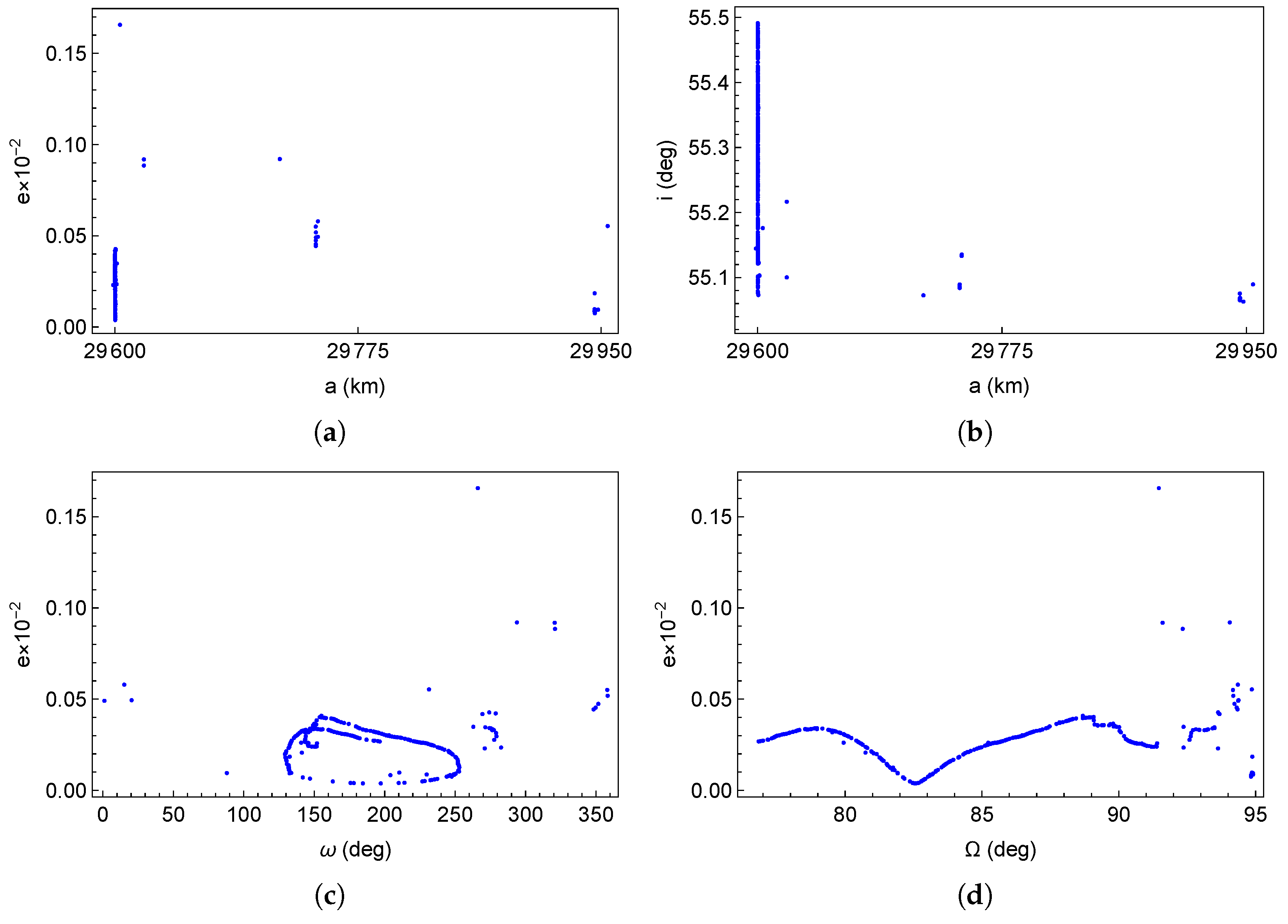
Figure 2.
Box-and-whisker plots showing the distance errors (km) of the best combinations of orbital variables for a time span of 30 days.
Figure 2.
Box-and-whisker plots showing the distance errors (km) of the best combinations of orbital variables for a time span of 30 days.
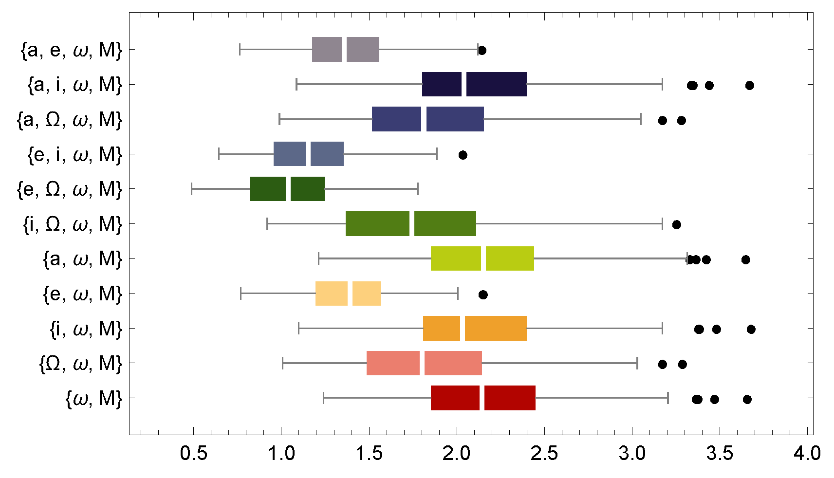
Figure 3.
Box-and-whisker plots showing the distance errors (km) of the best combinations of Hill variables for a time span of 30 days.
Figure 3.
Box-and-whisker plots showing the distance errors (km) of the best combinations of Hill variables for a time span of 30 days.
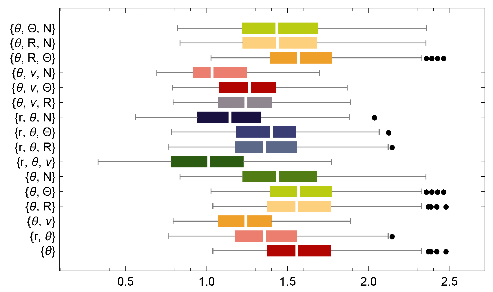
Figure 4.
Plot 50 of the 313 time series .
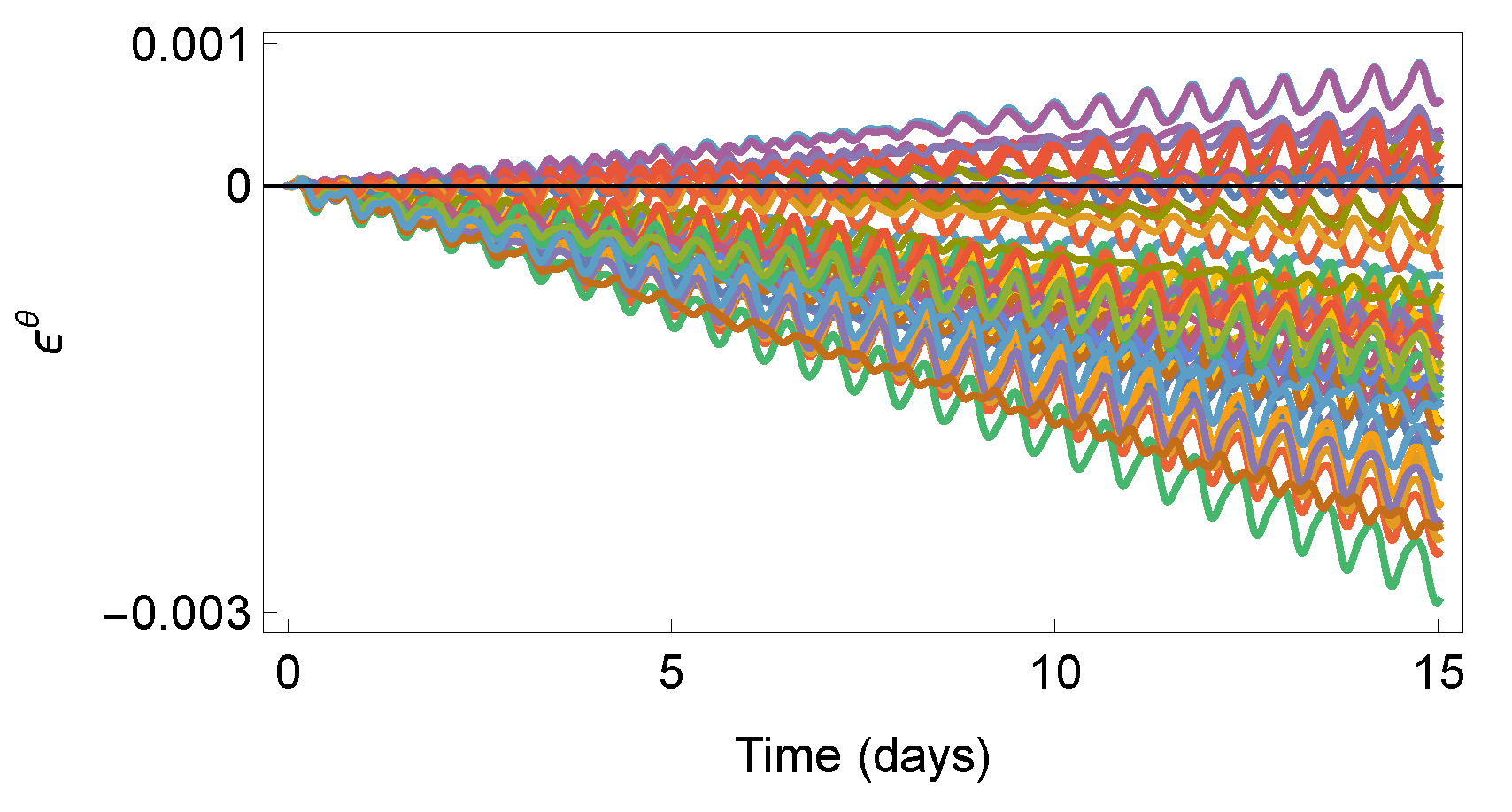
Figure 5.
Box-and-whisker plots showing distance errors (km) over a 30-day period. The ephemeris of the HSGP4 is simulated by replacing the argument of the latitude of SGP4 with the argument of the latitude of AIDA. (a) SGP4. (b) HSGP4 based on .
Figure 5.
Box-and-whisker plots showing distance errors (km) over a 30-day period. The ephemeris of the HSGP4 is simulated by replacing the argument of the latitude of SGP4 with the argument of the latitude of AIDA. (a) SGP4. (b) HSGP4 based on .
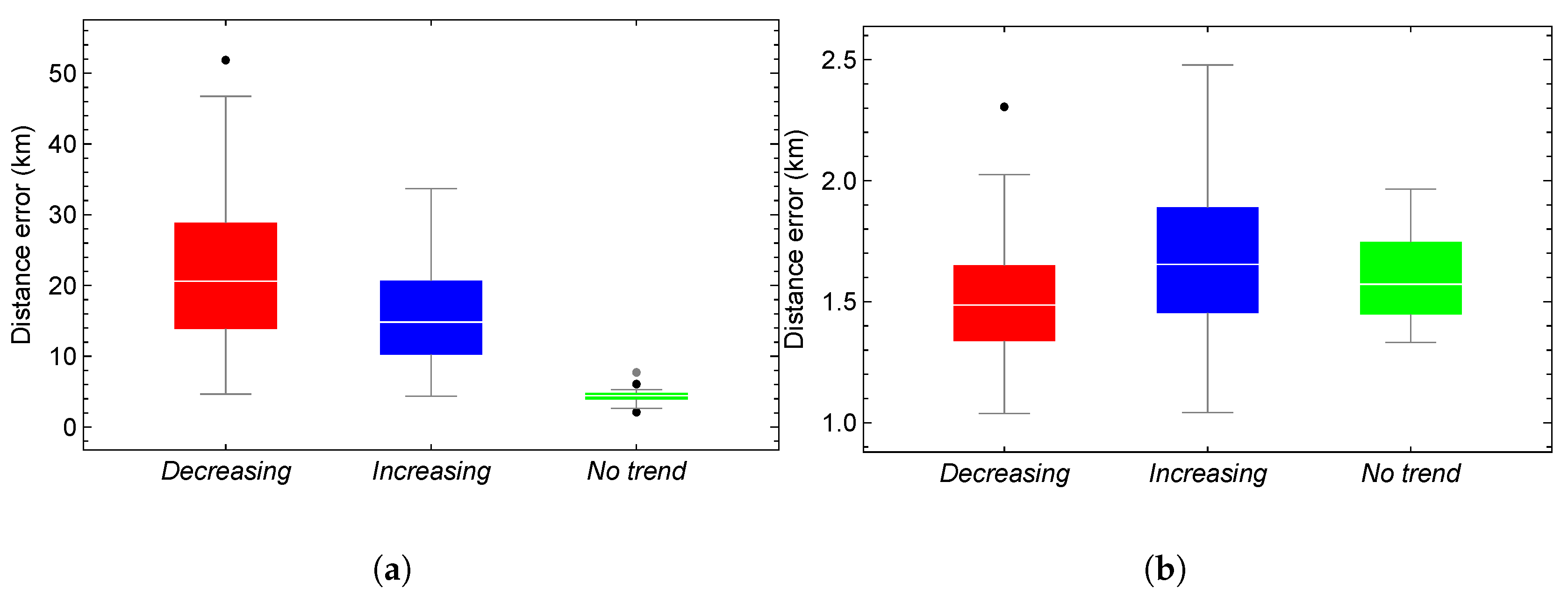
Figure 6.
Six time series. The orange dots represent the input vector; in red, the training set; in green, the validation set; and in blue, the test set.
Figure 6.
Six time series. The orange dots represent the input vector; in red, the training set; in green, the validation set; and in blue, the test set.

Figure 7.
Box-and-whisker plots of the distance error for the models using the mse (red) and mape (blue) loss functions at 2 and 4 days in the training stage and at 2, 4, 6, and 8 days in the testing stage.
Figure 7.
Box-and-whisker plots of the distance error for the models using the mse (red) and mape (blue) loss functions at 2 and 4 days in the training stage and at 2, 4, 6, and 8 days in the testing stage.
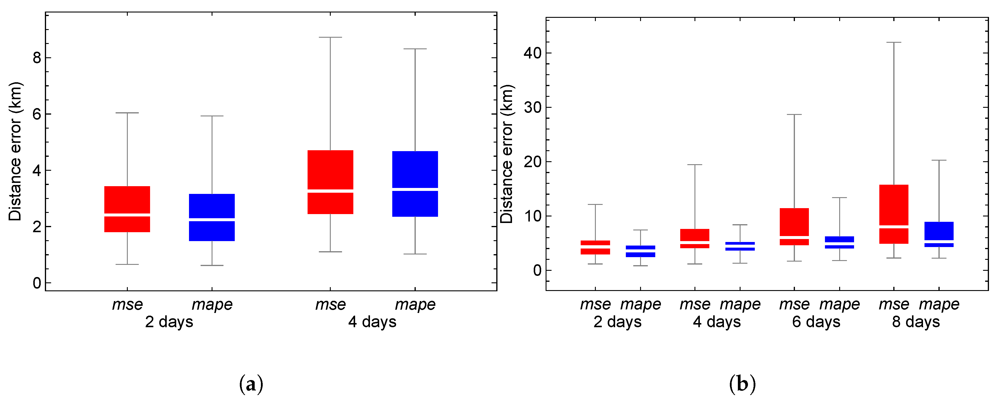
Figure 8.
Box-and-whisker plots of the distance error between the numerical propagator and HSGP4 were used to select the architectures presented in Table 5 and to reduce the distance error between the numerical propagator and SGP4.
Figure 8.
Box-and-whisker plots of the distance error between the numerical propagator and HSGP4 were used to select the architectures presented in Table 5 and to reduce the distance error between the numerical propagator and SGP4.
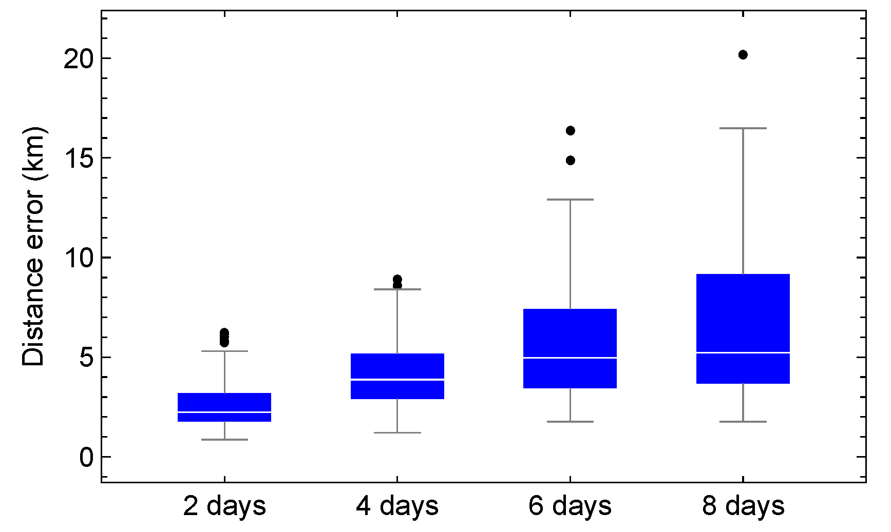
Figure 9.
Number of models for which the HSGP4 distance error is lower than the SGP4 distance error after 8 days of propagation.
Figure 9.
Number of models for which the HSGP4 distance error is lower than the SGP4 distance error after 8 days of propagation.
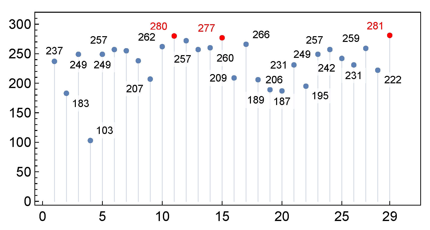
Figure 10.
Box-and-whisker plots of the distance error between the numerical and SGP4 propagators for the time series positive (PT, red), negative (NT, blue), or non-trend (NoT, green).
Figure 10.
Box-and-whisker plots of the distance error between the numerical and SGP4 propagators for the time series positive (PT, red), negative (NT, blue), or non-trend (NoT, green).

Figure 11.
Box-and-whisker plots of the distance error between the numerical and HSGP4 propagators, using models trained with architectures 11 (red), 15 (blue), and 29 (green) under a positive trend.
Figure 11.
Box-and-whisker plots of the distance error between the numerical and HSGP4 propagators, using models trained with architectures 11 (red), 15 (blue), and 29 (green) under a positive trend.
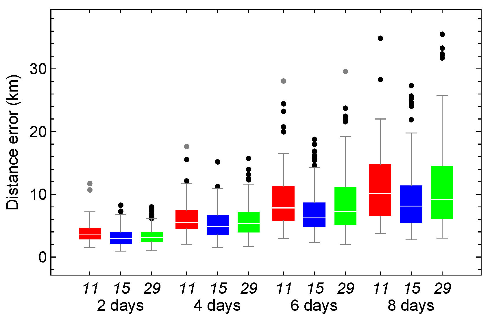
Figure 12.
Box-and-whisker plots of the distance error between the numerical and HSGP4 propagators, using models trained with architectures 11 (red), 15 (blue), and 29 (green) under a negative trend.
Figure 12.
Box-and-whisker plots of the distance error between the numerical and HSGP4 propagators, using models trained with architectures 11 (red), 15 (blue), and 29 (green) under a negative trend.
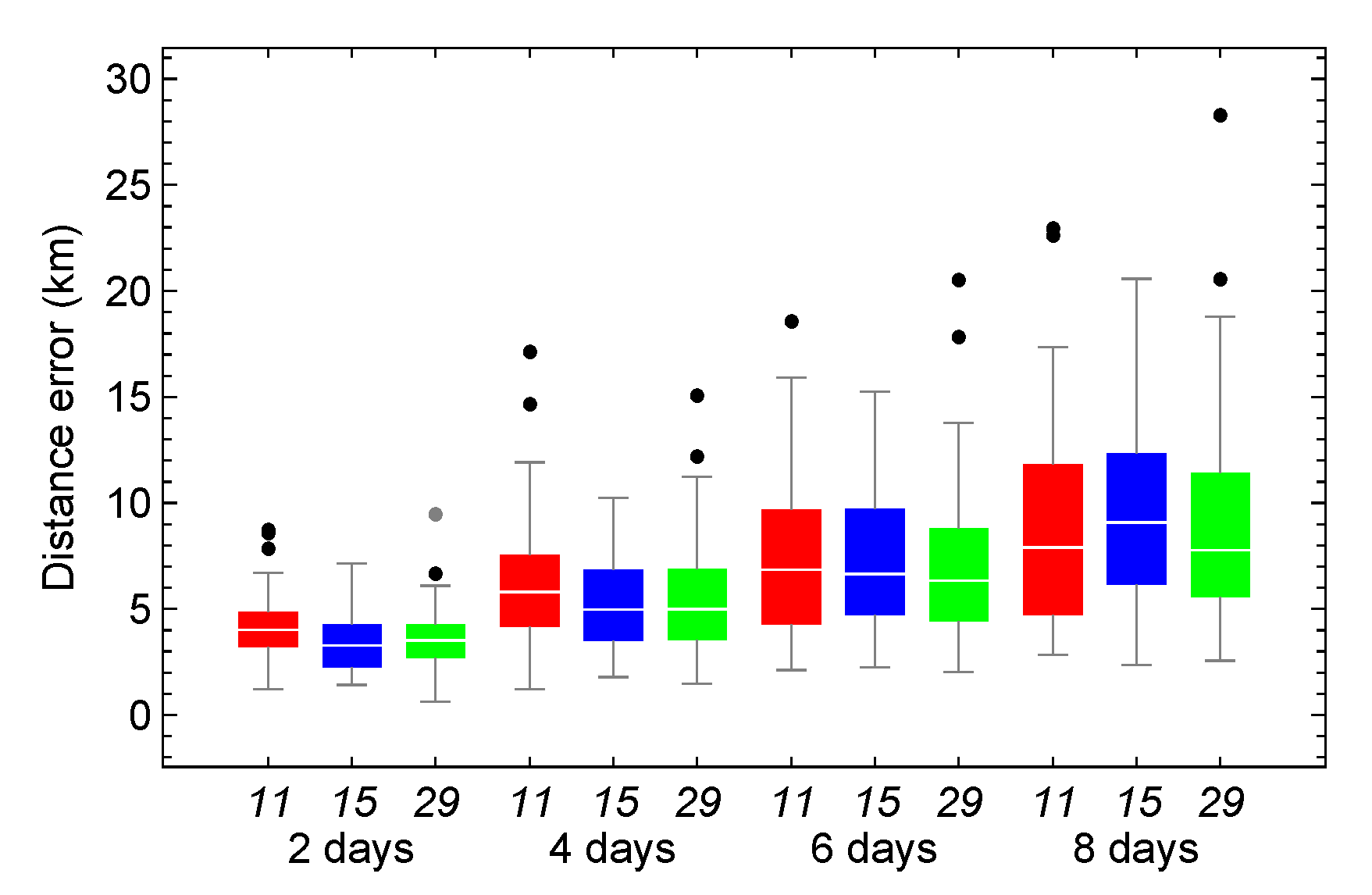
Figure 13.
Box-and-whisker plots of the distance error between the numerical and HSGP4 propagators, using models trained with architectures 11 (red), 15 (blue), and 29 (green) under a positive non-trend.
Figure 13.
Box-and-whisker plots of the distance error between the numerical and HSGP4 propagators, using models trained with architectures 11 (red), 15 (blue), and 29 (green) under a positive non-trend.
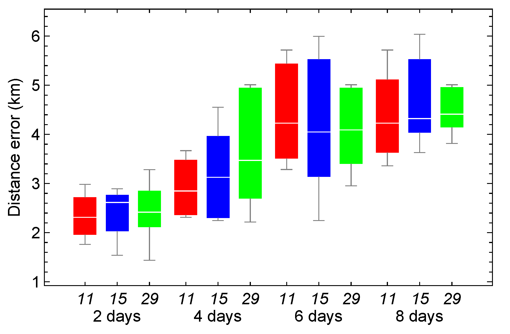
Figure 14.
The real values are shown in black. Predicted values are generated by models using architectures 11 (blue), 15 (green), and 29 (red).
Figure 14.
The real values are shown in black. Predicted values are generated by models using architectures 11 (blue), 15 (green), and 29 (red).
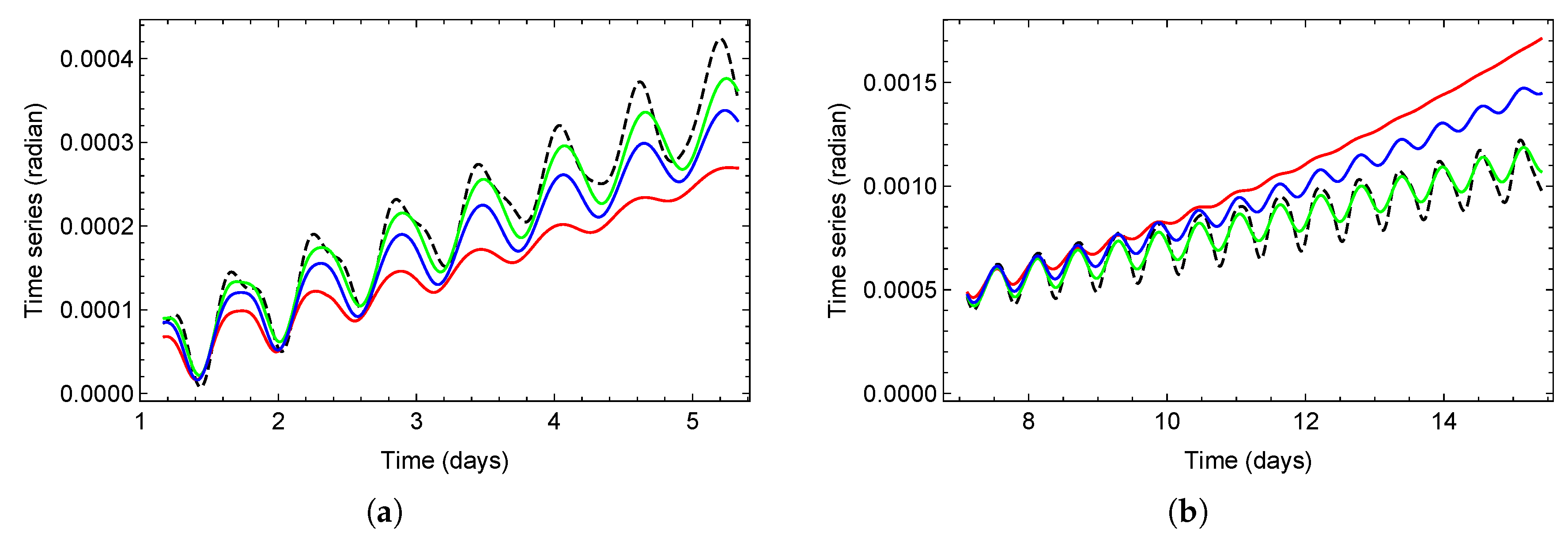
Figure 15.
Box-and-whisker plots of the distance error between the numerical and SGP4 propagators for the time series positive (PT, red), negative (NT, blue), or non-trend (NoT, green).
Figure 15.
Box-and-whisker plots of the distance error between the numerical and SGP4 propagators for the time series positive (PT, red), negative (NT, blue), or non-trend (NoT, green).
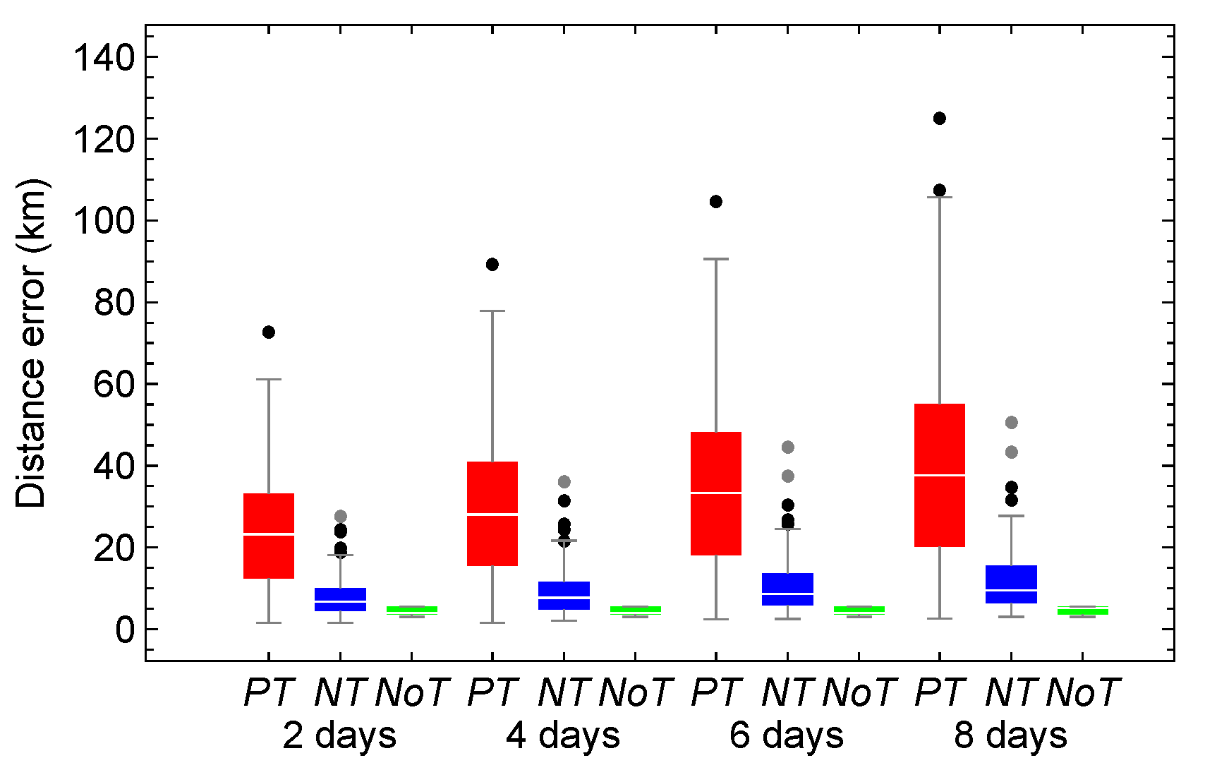
Figure 16.
Box-and-whisker plots of the distance error between the numerical and HSGP4 propagators, using models trained with architectures 11 (red), 15 (blue), and 29 (green). (a) Positive trend. (b) Negative trend. (c) Non-trend.
Figure 16.
Box-and-whisker plots of the distance error between the numerical and HSGP4 propagators, using models trained with architectures 11 (red), 15 (blue), and 29 (green). (a) Positive trend. (b) Negative trend. (c) Non-trend.
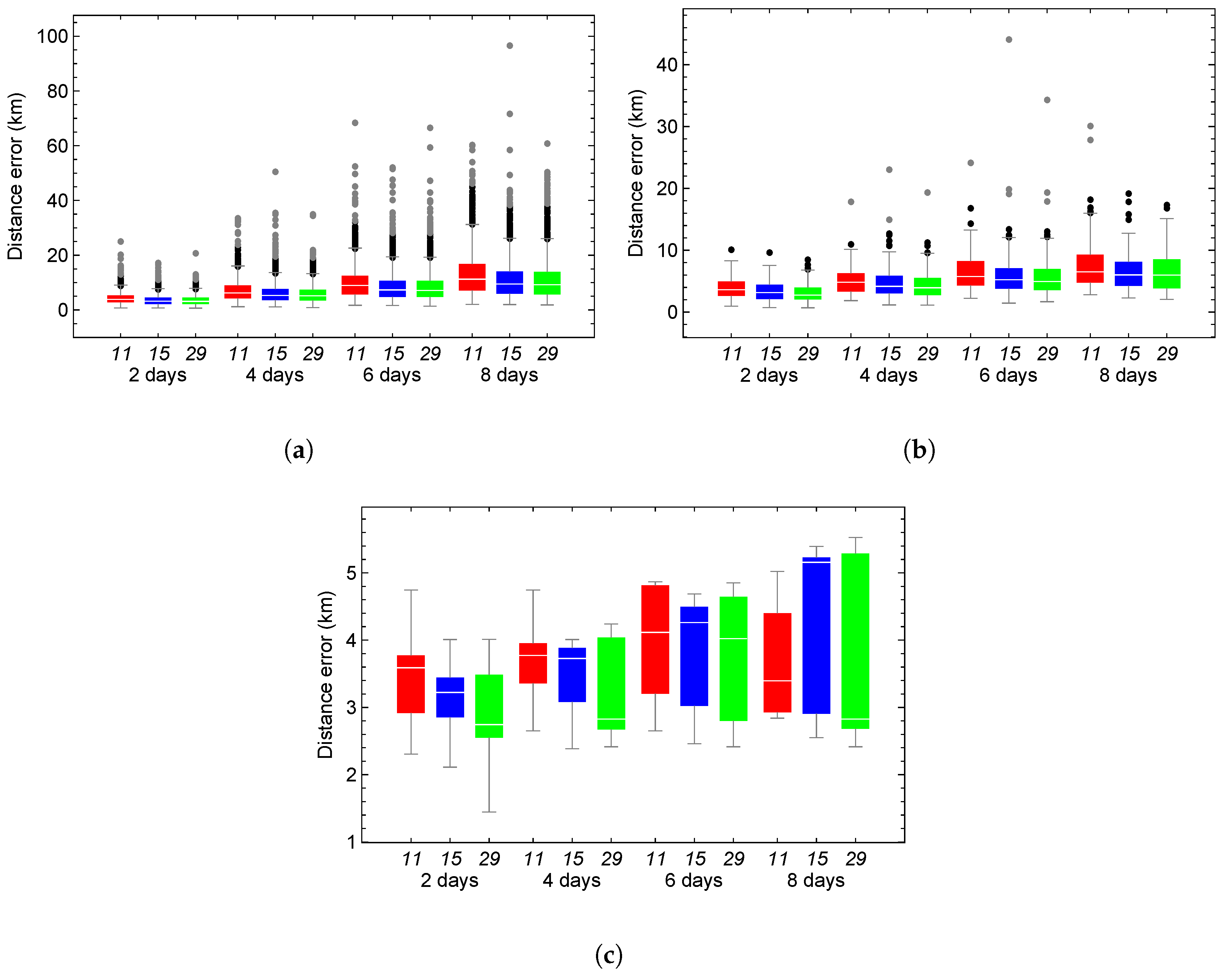

Table 1.
7-D hyper-parameter space () with their considered values. The activation functions considered are Linear, hyperbolic tangent (tanh), Rectified Linear Unit (relu), and Exponential Linear Unit (elu). The optimizers considered are Root Mean Square Prop (rmsprop), Adaptive Delta (adadelta), Adaptive Moment Estimation (adam), and Nesterov-accelerated Adaptive Moment Estimation (nadam). The loss functions considered are the mean squared error (mse), mean absolute error (mae), mean absolute percentage error (mape) and mean square logarithmic error (msle).
| Hyperparameters | Range of values |
|---|---|
| Batch size | 64, 128, 256, 512 |
| Hidden layers | 1, 2, 3 |
| Number of neurons in the first hidden layer | 8, 16, 32, 64, 128, 256 |
| Activation Functions | linear, tanh, elu, relu |
| Optimizers | rmsprop, adadelta, adam, nadam |
| Loss function | mse, mae, mape, msle |
| Learning rate | 0.001, 0.0001, 0.00001 |
Table 2.
Number of models with the lowest RMSE during training and testing.
| Architectures | Training | Testing |
|---|---|---|
| mae | 403 (18.35%) | 510 (23.22%) |
| mape | 780 (35.52%) | 880 (40.07%) |
| mse | 837 (38.12%) | 581 (26.46%) |
| msle | 176 3(8.01%) | 225 (10.25%) |
Table 3.
Number of models where the distance error of HSGP4 is less than the SGP4 error after 8 days in the testing set, and the average computational time of the training of the model. Of the 2,196 models, 102 have 1 hidden layer, 420 have 2 hidden layers, and 1,674 have 3 hidden layers.
Table 3.
Number of models where the distance error of HSGP4 is less than the SGP4 error after 8 days in the testing set, and the average computational time of the training of the model. Of the 2,196 models, 102 have 1 hidden layer, 420 have 2 hidden layers, and 1,674 have 3 hidden layers.
| Hidden layers | Test | Time (min) |
|---|---|---|
| 1 | 36 (35.29%) | 2.83 |
| 2 | 247 (58.81%) | 3.18 |
| 3 | 1122 (67.03%) | 3.60 |
Table 4.
Distribution of models chosen by the smallest error in distance, discriminated by learning rate value and by forecast set. The final column shows the median modeling time for each learning rate.
Table 4.
Distribution of models chosen by the smallest error in distance, discriminated by learning rate value and by forecast set. The final column shows the median modeling time for each learning rate.
| LR | Train | Test | Median modelling time (sec) |
|---|---|---|---|
| 1e-05 | 817 (44.21%) | 290(15.69%) | 295.61 |
| 1e-04 | 647 (35.01%) | 794 (42.97%) | 267.92 |
| 1e-03 | 384 (20.78%) | 764 (41.34%) | 266.42 |
Table 5.
Best architectures that minimize the distance error after 8 propagation days.
| Id | BatchSize | Neu First HL | Optimizer | ActFun1 | AtFun2 | Freq |
|---|---|---|---|---|---|---|
| 1 | 512 | 8 | Nadam | tanh | elu | 2 |
| 2 | 256 | 8 | Adam | tanh | elu | 1 |
| 3 | 64 | 256 | Adam | tanh | tanh | 1 |
| 4 | 64 | 16 | Adadelta | relu | elu | 1 |
| 5 | 128 | 256 | Nadam | relu | elu | 1 |
| 6 | 256 | 64 | Adam | tanh | tanh | 1 |
| 7 | 128 | 32 | Nadam | tanh | elu | 1 |
| 8 | 128 | 16 | Adam | linear | linear | 1 |
| 9 | 512 | 128 | Nadam | linear | relu | 1 |
| 10 | 128 | 64 | Adam | elu | tanh | 1 |
| 11 | 64 | 16 | Rmsprop | tanh | elu | 1 |
| 12 | 256 | 128 | Adam | linear | linear | 1 |
| 13 | 128 | 128 | Adam | tanh | tanh | 1 |
| 14 | 256 | 128 | Nadam | linear | elu | 1 |
| 15 | 256 | 64 | Nadam | linear | tanh | 1 |
| 16 | 256 | 16 | Adam | elu | elu | 1 |
| 17 | 512 | 128 | Adam | elu | elu | 1 |
| 18 | 256 | 16 | Adam | linear | linear | 1 |
| 19 | 512 | 16 | Adam | relu | elu | 1 |
| 20 | 256 | 16 | Adam | tanh | elu | 1 |
| 21 | 64 | 128 | Nadam | relu | elu | 1 |
| 22 | 256 | 16 | Nadam | relu | tanh | 1 |
| 23 | 64 | 16 | Nadam | linear | elu | 1 |
| 24 | 256 | 256 | Nadam | linear | linear | 1 |
| 25 | 64 | 256 | Adam | relu | linear | 1 |
| 26 | 256 | 32 | Adam | elu | elu | 1 |
| 27 | 64 | 64 | Adam | linear | tanh | 1 |
| 28 | 256 | 32 | Adam | tanh | linear | 1 |
| 29 | 256 | 32 | Nadam | linear | tanh | 1 |
Table 6.
Number of methods reducing SGP4 error, grouped by time series trend.
| Trend | 2 days | 4 days | 6 days | 8 days |
|---|---|---|---|---|
| Positive | 58 | 58 | 54 | 51 |
| Negative | 54 | 54 | 53 | 46 |
| Non-trend | 56 | 51 | 50 | 44 |
Table 7.
Number of cases for each architecture where the error associated with HSGP4 is greater than that of SGP4 for the Galileo satellite (NORA ID 40545). The number of positive, negative, and non-trend time series are 169, 118, and 26, respectively.
Table 7.
Number of cases for each architecture where the error associated with HSGP4 is greater than that of SGP4 for the Galileo satellite (NORA ID 40545). The number of positive, negative, and non-trend time series are 169, 118, and 26, respectively.
| Trend | Architecture | 2 days | 4 days | 6 days | 8 days |
|---|---|---|---|---|---|
| Positive | 11 | 33 | 33 | 33 | 36 |
| 15 | 20 | 24 | 30 | 31 | |
| 29 | 19 | 24 | 28 | 36 | |
| Negative | 11 | 45 | 40 | 46 | 51 |
| 15 | 20 | 22 | 27 | 30 | |
| 29 | 28 | 28 | 33 | 37 | |
| Non-trend | 11 | 22 | 22 | 21 | 19 |
| 15 | 17 | 20 | 19 | 19 | |
| 29 | 19 | 20 | 20 | 21 |
Table 8.
Each selected architecture contains two hidden layers, a learning rate of 1e-4, a linear activation function in the output layer, and uses the mape as the loss function.
Table 8.
Each selected architecture contains two hidden layers, a learning rate of 1e-4, a linear activation function in the output layer, and uses the mape as the loss function.
| Id | BatchSize | Nº Neu 1º HL | Optimizer | ActFun1 | AtFun2 |
|---|---|---|---|---|---|
| 11 | 64 | 16 | Rmsprop | tanh | elu |
| 15 | 256 | 64 | Nadam | linear | tanh |
| 29 | 256 | 32 | Nadam | linear | tanh |
Table 9.
Number of cases for each architecture where the error associated with HSGP4 is greater than that of SGP4 for the Galileo satellite (NORA ID 38857). The number of positive, negative, and non-trend time series are 1447, 227, and 9, respectively.
Table 9.
Number of cases for each architecture where the error associated with HSGP4 is greater than that of SGP4 for the Galileo satellite (NORA ID 38857). The number of positive, negative, and non-trend time series are 1447, 227, and 9, respectively.
| Trend | Architecture | 2 days | 4 days | 6 days | 8 days |
|---|---|---|---|---|---|
| Positive | 11 | 15 | 40 | 60 | 90 |
| 15 | 11 | 32 | 79 | 129 | |
| 29 | 14 | 32 | 68 | 138 | |
| Negative | 11 | 19 | 27 | 34 | 41 |
| 15 | 12 | 38 | 51 | 64 | |
| 29 | 16 | 38 | 53 | 65 | |
| Non-trend | 11 | 0 | 1 | 2 | 5 |
| 15 | 0 | 2 | 3 | 4 | |
| 29 | 0 | 0 | 1 | 4 |
Disclaimer/Publisher’s Note: The statements, opinions and data contained in all publications are solely those of the individual author(s) and contributor(s) and not of MDPI and/or the editor(s). MDPI and/or the editor(s) disclaim responsibility for any injury to people or property resulting from any ideas, methods, instructions or products referred to in the content. |
© 2026 by the authors. Licensee MDPI, Basel, Switzerland. This article is an open access article distributed under the terms and conditions of the Creative Commons Attribution (CC BY) license (http://creativecommons.org/licenses/by/4.0/).
Copyright: This open access article is published under a Creative Commons CC BY 4.0 license, which permit the free download, distribution, and reuse, provided that the author and preprint are cited in any reuse.


