Submitted:
04 January 2026
Posted:
05 January 2026
Read the latest preprint version here
Abstract
Customer-grade affordable active radon monitors occupy a growing segment of the radon measurement market. This is no surprise given the fair price, easy operation, versatile applicability and reasonable performance. A relatively recent member of the family is the Aranet Radon-plus, made by a Latvian company. Two devices were tested in parallel together with one RadonEye, an already well established monitor of this class. In comparison with the latter, the Aranet has a somewhat lower sensitivity, but additional useful features, namely a time stamp and measurement of meteorological parameters. Operability via Smartphone and Bluetooth is very similar. One difficult issue is data smoothing that introduces artificial autocorrelation of reported data which is problematic in certain applications. In this paper, several experiments under different exposure scenarios (indoors, outdoors, thoron, moving) to assess the performance of the Aranet and some considerations regarding counting statistics are presented.
Keywords:
Aranet radon monitor
; ambient radon measurement
; counting statistics
1. Introduction
For certain applications involving measurements of radon (Rn)[1] concentration, active monitors are required which deliver results in near real-time. These applications are in the field of radiation protection and environmental research. In the first case, one aims to verifying if people are not exposed to harmful radon concentrations and compliance with regulatory limits. In the second case, Rn is used as a tracer of environmental processes mainly in atmospheric and hydrological sciences and for studying air exchange dynamic in buildings or caves, and the like. (Since there is plenty of literature about Rn as tracer there is no need for further discussion here.)
For some years, affordable customer grade active Rn monitors are available on the market. Their price and their ease of usage are such that they can compete with traditional passive track-etch or SSNTD detectors for longer-term indoor Rn assessment. In addition, active monitors which yield sufficiently resolved time series can be used in a time discriminating mode, which is relevant mainly in the context of characterization of work places which have specified operation times. Given diurnal Rn cycles and the influence of ventilation, mean concentrations during working hours and full days can be very different[2]. They are also useful if Rn characterisation of a house is needed quickly for example in the case of house transactions. Methods for checking compliance with reference levels based on short-time tests have been suggested by [1,2,3].
If the limitations of these devices are respected, they can also be applied in scientific contexts. Tests like the ones reported here are intended to strengthen QA and explore the limits of the instruments.
Due to their low cost and easy usage, customer-grade Rn monitors have a great potential in Citizen Science [4] and could increase the number of Rn tests by individual citizens independently of public screening programs. This has been emphasized by [1,2]. One of the objectives of this paper is to show how relevant QA-related experiments can be performed with simple means and independently of dedicated radon laboratories, whose services are usually very expensive.
One relatively new member of the family of customer-grade active Rn monitors is the Aranet Radon Plus, produced by the Latvian company SAF tehnika [5]. Two devices were used for the tests reported in this paper. To my knowledge, so far no performance and QA tests have been published about the Aranet monitor. This is different from RadonEye, Correntium and other customer grade / low-cost Rn monitors, which have been subjected to QA tests by a number of authors.
2. Materials and methods
2.1. The Aranet Monitor
The monitor has an ionization chamber with 137 cm³ volume as detector. The nominal sensitivity of the Aranet is 1.19 cpm / 100 Bq/m³ [8] (recalculated from the value called efficiency in the document), slightly lower than the one of the somewhat cheaper RadonEye, 1.35. For comparison, professional-grade monitors (almost two orders of magnitude more expensive): Alphaguard: 5.0, Rad-8: 2.2.
The Aranet monitor can be connected to a Smartphone app through Bluetooth which allows easy controlling the device, visualizing the data and downloading them as csv and xlsx files.
The nominal counting interval is 10 minutes. Data are stored for 35 days only (Radon Eye: 1 year). The device is operated by 2 AA batteries which last for 3.3 years if Bluetooth is on, according to the manufacturer [8] (Radon Eye: external power).
A feature that distinguishes the Aranet from the RadonEye (basic model) is the time stamp (retrieved from a connected Smartphone) and measurement of temperature, humidity and air pressure. The results are included as separate columns in the report file. If the humidity exceeds 90%, no Rn values are reported. The meteorological data will not be discussed further in this paper.
The two Aranet monitors investigated here were purchased in late October 2025. Their serial numbers are 503700209291, product number 3318B and 503700209285, product number 33185. In this paper the monitors are referred to by the product number, because this is also used in the report file names generated by the device. An Aranet monitor costs about 220 € (October 2025), compared to about 180 € for a RadonEye.
2.2. Low-Pass Filtering of the Raw Data
The Rn concentration data reported on the screen and recorded in the downloadable data files are 10 minute values, averaged over the last hour, that is, the moving average or sliding mean of the last 6 values [personal communication]. Access to raw count data within the 10 minute counting interval is not possible. This results in introducing artificial autocorrelation of data or in other words, artificial statistical dependence within each sub-series of 6 data. Let x(t) the raw concentrations or count numbers, where t is counted in units of 10 minutes and y(t), the reported concentration at time t. Then,
y(t) = (1/6) Σi=0…5 x(t-i).
After 6 time steps, i.e., 1 hour, this effect is removed, meaning that y(t) and y(t-6) are not correlated due to the averaging (as a property of the actual process they can still be). For statistical analysis, one should therefore only use partial series {y(t), y(t+6),…} consisting of every sixth record. The autocorrelation in this series is the one of the true Rn concentration in which one is interested (plus possibly a contribution generated by device inertia). The information that is lost using such partial series is a possible dynamic within the contiguous one hour intervals, which is usually little relevant in radon studies, if present at all due to the inertia of natural systems which acts as a “natural smoother”.
The probable reason why this procedure has been introduced by the manufacturer is to smooth away statistical fluctuations to some degree.
If we assume the sensitivity 1.19 cpm per 100 Bq/m³, we find that in average, 1 Bq/m³ generates 0.714 counts per hour. As an example, 14 Bq/m³ yield 10 counts per hour. Due to Poisson statistics, the variance within 1 hour is also 10 and the standard deviation (SD) equals √10=3.16 counts which corresponds to 4.4 Bq/m³. This results in a variability expressed as coefficient of variation CV=4.4/14 = 0.32.
In principle, the series can be de-convoluted. y(t) can be understood as a convolution, y(t) = (x∗h)(t), with h – a trailing rectangular filter of length six units, h(0)=…=h(5)=1/6, else=0. In Fourier space, Y(s) = X(s) H(s), where the capital letters denote the Fourier transformed variables, X(s) = F x(t). Therefore, theoretically, x(t) can be retrieved as F-1 Y(s)/H(s). (For rectangular filters, H(s) is given by the cardinal sine function sinc(s).)
The autocorrelation function for lag u, ACFy(u) = (y∗y)(u) = x∗h∗x∗h ∝ (h∗h)(u) (up to factors). Its shape near u=0 is given by h∗h, which is easily found to equal 1-u/6, u∈[0,5], else =0, i.e., a linear decrease. This behaviour is characteristic for moving average low-pass filters and can be used for diagnosis, like in section 3.4.
In practice, for discrete time series, a simple deconvolution method is as follows:
Define y(i) the recorded convoluted value at t=i and x(i) the deconvoluted value; y(0) = (x(0)+x(-1)+…+x(-5))/6.
Define Δy(0) := y(0) – y(-1) = (x(0) – x(-6))/6. Hence, x(0) = 6 Δy(0) + x(-6) which can be processed recursively. The problem is that the thus recovered series x(i) – or better: estimated series x’(i) - is very noisy, as will be demonstrated below. The x’(i) can be <0 which is physically impossible; these cases are forcibly set to zero.
As a consequence, (x’(i) +… + x’(i-5))/6 ≥ y(i) in general. The x’(i) are therefore regularized by multiplication with y(i)/[(x’(i) +… + x’(i-5))/6].
2.3. Experiments
The experiments described in the following were performed under realistic ambient conditions but not under laboratory conditions. This distinguishes this study, similar to [6,7], from most laboratory based QA related work. Tests under ambient conditions usually lack sensitivity and specificity of lab-based tests, that is, are less accurate, but are more indicative of performance under “field use”. They are stronger in the sense that if a device performs well under ambient, that is noisy and overall little controllable conditions, it may be more reliable than one that passes “only” QA checks in the calibration chamber. At the same time, ambient-based tests are weaker in the sense that they may not be able to detect small deviations from an ideal behaviour. In the terminology of ROC analysis, the AUC index of tests under ambient conditions can be expected to be lower than under lab conditions, due to the inevitably involved nuisance factors in the former.
One aspect of the work – in the spirit of Citizen Science - is that the experiments can be performed without laboratory equipment and particular training and experimental skill.
2.3.1. Parallel Measurements
a) Same location
Parallel measurements with two Aranet and one RadonEye monitor were performed indoors for 10 days and outdoors for 16 days. The set-up is shown in Figure 1. The measurement location in Berlin, Germany, has been described in detail in [6].
The RadonEye used as parallel monitor has the serial number HG04RE000641. It has been purchased in May 2024 and never been exposed to Rn concentrations higher than several 10 Bq/m³. Therefore it can be assumed that its internal background count rate is negligible. (The background count rate is caused by deposition of long-lived Rn progeny in the ionization chamber and electronic noise.) Indoor exposure was between 24 Oct and 3 Nov 2025, outdoors 3 to 20 Nov 2025.
b) Different nearby locations
A second series of measurements was performed as follows:
1. RadonEye: Indoors, as in Figure1, left; 2. Aranet 3318B: indoors, on a bookshelf, ca. 1.5 m above ground (Figure 2, left), about 5 m away from the RadonEye; 3. Aranet 33185: Staircase of the same building (Figure 2, right), separated from the room with monitors 1. and 2. by a relatively well isolated airtight door. The monitors were not moved or shaken during the experiment. The duration was from 20 Nov to 7 Dec 2025 during the heating season.
2.3.2. The Radon Profile During a Journey
The two Aranet monitors were stowed in their cardboard boxes and carried in a back bag during a bus and train journey from Berlin to Vienna, 9 Dec 2025. The bag was located in the luggage compartment of the bus Berlin - Dresden – Prague and on the overhead rack in the train Prague – Vienna. The bus ride goes along motorways, the train along the Franz Josefs-Bahn Prague – Tabor – Ceske Velenice (Czech/Austrian border) – Eggenburg – Tulln – Vienna. This slow train was chosen because it crosses the Bohemian massif, a region of high geogenic radon potential which might be visible in the radon readings. One can assume that in the bus and in the train the monitors are essentially exposed to outdoor radon. Vibration may deteriorate the performance.
2.3.3. Sensitivity to Thoron
The objective of this experiment was to verify the Aranet’s anticipated sensitivity against thoron. The bottom of a plastic container was covered with concentrated monazite sand and one Aranet positioned on top, separated by space holders to avoid contamination of the device, Figure 3. The concentration time series was recorded and the decay analyzed in analogy to the same experiment performed with a RadonEye [7]. (Monazite sand may not be available easily – in our case it came from Brazil – but in some countries, equally usable thorium containing Auer-Welsbach mantles can still be purchased openly, but they should also be used with caution given radiation protection issues[3].)
2.3.4. Internal Background
An upper limit of the internal background whose origins is mainly electronic noise and possibly traces of radium contained in components of the device was assessed in an experiment similar to the thoron experiments. The bottoms of plastic food containers labelled as being made of polypropylene (“PP”) were filled with freshly heated activated charcoal which removes Rn from the chamber atmosphere very efficiently and the monitors set above. Two / three containers one above the other were used as double / triple Rn barrier. The joints of the lids of the plastic containers were additionally sealed with Teflon tape and further with insulating tape from the hardware shop. However, PP is known to have lower diffusion resistance for radon than for example PVC.
3. Results
3.1. Counting Statistics
3.1.1. Confidence Intervals
We assume the reported values to be pure Poisson variates and the detector sensitivities the nominal ones. This means 1 count per 10 minutes = 8.403 Bq/m³ and 1 count per 1 hour = 1.401 Bq/m³.
C.I. = (0.5 χ²(α/2, 2 x) ; 0.5 χ²(1-α/2, 2(x+1))),
α - the confidence level, here α=0.05 chosen, and x - degrees of freedom = count number per interval (10 minutes or 1 hour)[4]. (The same formula is given in the Wikipedia entry “Poisson distribution”.) See also section 4.2 in [6][5]. In Figure 4 the count numbers were converted into Rn concentrations.
3.1.2. Decision Threshold and Detection Limit
Decision threshold x* and detection limit x# are calculated according to Currie as in sec. 4.2 in [6], but with a correction for small background count numbers x0, again according to IAEA Tab. 4, p. 22 in [11], x0 → x0+1.
x* = kα √(2(x0+1))
x# = kα² + 2kα √(2(x0+1))
For more refined methods, see [11,12], appendix IV [13]. For α=0.05, kα=1.645. Also the uncertainty of the sensitivity is unknown and ignored here, which would otherwise enter in the calculations. Decision threshold and detection limit in terms of activity concentration, in dependence of the background rate, are shown in Figure 5. A particular background rate in terms of counts during different intervals (10 min or 1 h) corresponds to different concentrations and different DL and LLD in terms of concentrations.
We do not know the background x0; like in [6] we can assume the x0 rate = 1 cph or 1.4 Bq/m³ which may be realistic for new or little exposed detectors, otherwise probably an underestimation.
3.1.3. Constancy of the Counting Interval
The nominal counting interval Δt equals 10 minutes. However, in the records some instances of 9 minute intervals occur, Table 1. In the investigated series (the indoor series, sec. 3.4), 4 such instances occurred in each series of 10 days, giving a frequency 0.28% or in average approximately one case in every 9.6 hours. These events do not happen simultaneously in the series. A temporal pattern of these irregularities could not be noticed. Deviation from the nominal interval is too low to be of practical concern in most applications.
3.2. Transient Behaviour
a) Abrupt change of the Rn concentration
A transient between higher (indoor) and lower (outdoor) exposure is shown in Figure 6. The transient phase lasted for about 2 hours (until about 12:00) before the concentrations reached the new levels, about 5 Bq/m³ (starting from about 20 Bq/m³ before 10:00). The opposite transients, outdoors → indoors are shown in Figure 7.
b) Rn profile during a journey
The radon concentration time series recorded by the two Aranet monitors is shown in Figure 8. Like above the 10 min- and 1 h- values are plotted.
The coincidence between the Aranet readings is very poor. In particular indoors until 10:00 one would have expected better coincidence. Soon after leaving the house at 10:00 both monitors levelled to typical outdoor concentrations, about 5 Bq/m³. The transients look similar to the ones shown in Figure 6 and Figure 7. The Rn concentrations increased somewhat to about 10 – 15 Bq/m³ after 14:00 when the region of the Ore mountains South of Dresden was passed, which is known for its elevated geogenic Rn potential. This higher level persisted when passing the territory of the Czech Republic and Northern Austria and peaked at about 20 Bq/m³ around 19:00 to 21:00 when the Southern Bohemian Massif was passed. This is a granitic region known for high radon potential and indoor Rn concentrations.
c) Detector movement and vibration
After relocating the two Aranets between two nearby locations in the same atmosphere (Berlin outdoors), although done gently, the records show a substantial spike which seems out of normal statistical fluctuation, Figure 9. The spike is recorded in the 10 min-series with a delay of about ½ hour. The monitors were relocated because it was thought that at the new location they were less susceptible to humidity, but subsequently it showed that this was not the case.
3.3. High Humidity
Episodes of high nocturnal humidity are shown in Figure 10. Humidity ≥ 90% leads to the interruption of Rn recording. Whether also measuring is interrupted, or only recording, cannot be inferred from the recorded data. After the humidity dropped below 90% it took the monitors between 2 and 3 hours to recover and to resume recording Rn concentration values.
3.4. Verification of the Low-Pass Filtering and Deconvolution
The indoor series (Figure 12) were used to verify the effect of low-pass filtering. To this end the autocorrelation functions (ACF) of the filtered and non-filtered series were computed. The ACF plots are shown in Figure 11. As a result of 6-lag = 1 hour moving average filtering, the ACF of the 10-min values show the typical decay up to 6 lags and subsequent smooth undulation. The 1-hour values do not show this behaviour: from the first lag onwards only the ACF of the investigated process – Rn concentration - is revealed.
Figure 11.
Autocorrelation (ACF) plots of filtered 10 min-values (left) and 1 h-values (right).
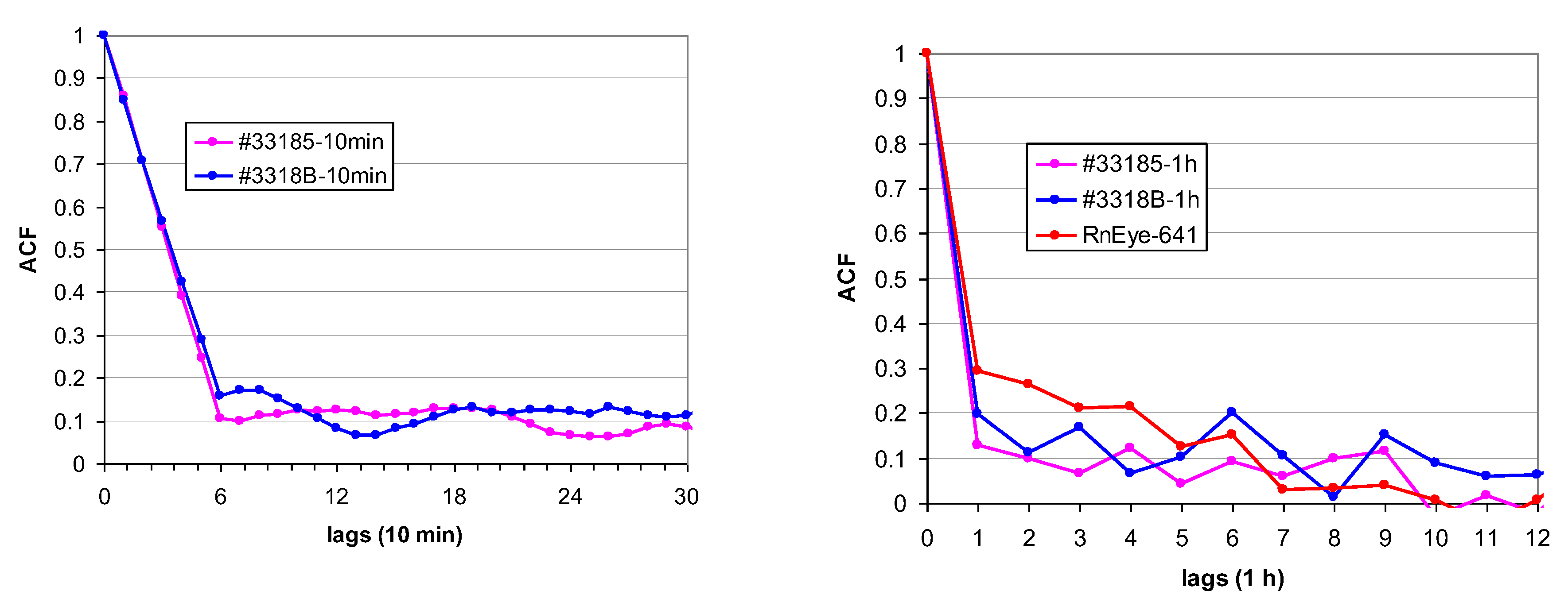
Figure 12.
Input series y(i) and deconvoluted x’(i).
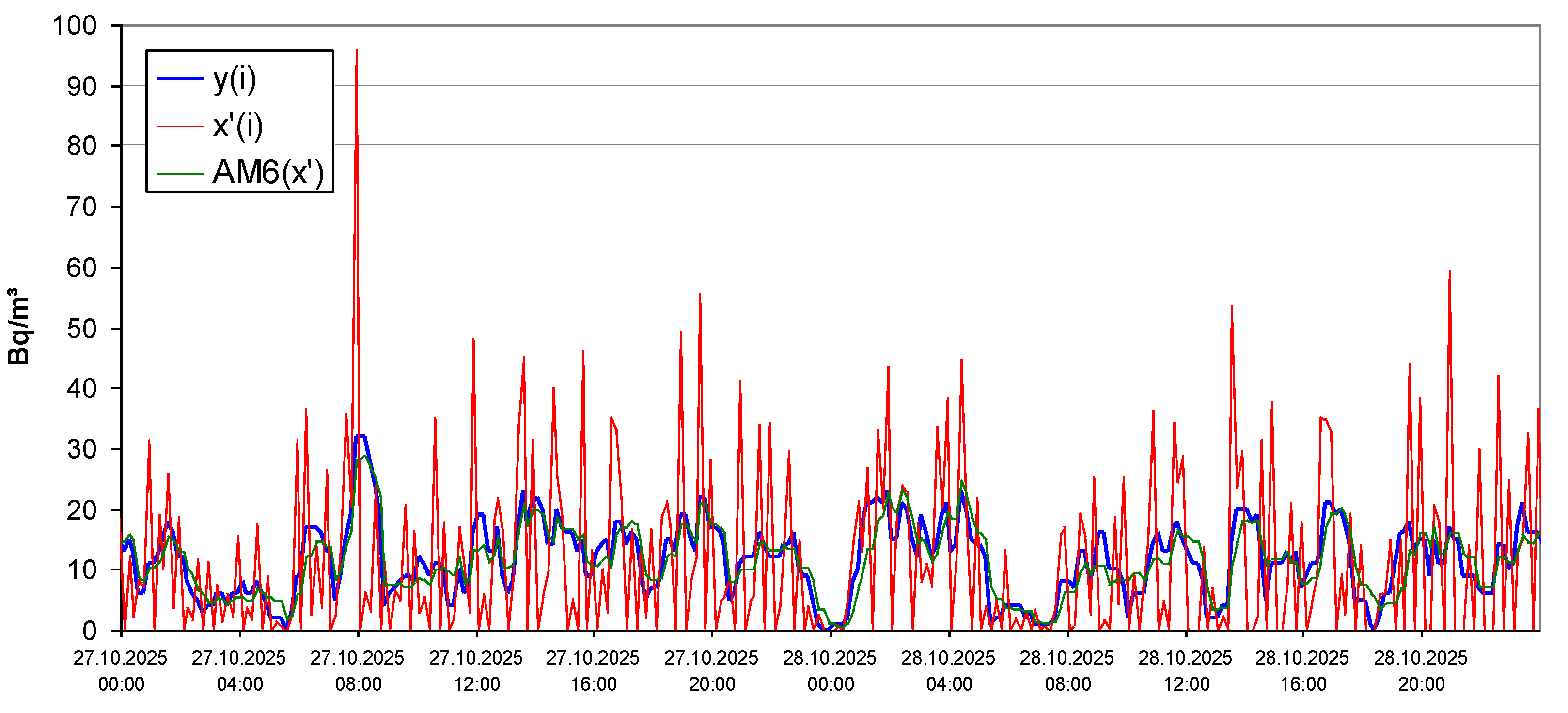
Figure 11, right, also shows that estimating the decorrelation time τ from the ACF plots of the Aranet series is difficult, while the one of the RadonEye yields a τ of about 5 hours quite clearly. τ is defined here as the number of lags after which the ACF drops below the 0.05 confidence limit (0.158, not shown in the graph). The probable reason is the lower sensitivity of the Aranet whose dynamic is more affected by statistical noise. Feeding longer series into the ACF analysis would probably allow revealing τ also with the Aranet monitor.
A deconvoluted series, following the algorithm given in section 2.2, is shown in Figure 12. The curve AM6(x’) := (x’(i)+…+x’(i-5))/6 is close to y(i) and shows that regularization is efficient. It should be noted that x’ is not the (unknown) “true” Rn concentration in a 10 min interval, but the true one subject to Poisson uncertainty.
3.5. Parallel Measurements
a) Parallel measurements at one location
For the analysis and the time series plots, Figure 13 and Figure 14, those Aranet results were used whose time stamp coincided with the one of the RadonEye, that is, every sixth of the Aranet records. This way the low-pass filtering problem, addressed above, is avoided. In practice, time coincidence can be achieved only up to a few minutes, because perfect synchronization of the measurement intervals seems impossible. Basic statistics are given in Table 2 and Table 4, the correlation matrix in Table 3 and Table 5.

Table 2.
Basic statistics of the Rn concentrations measured with three monitors in parallel; Berlin indoors. AM – arithmetic mean; SD, SE – standard deviation and error; CV – coefficient of variation = SD/AM; Δt – duration of the measurement period.
Table 2.
Basic statistics of the Rn concentrations measured with three monitors in parallel; Berlin indoors. AM – arithmetic mean; SD, SE – standard deviation and error; CV – coefficient of variation = SD/AM; Δt – duration of the measurement period.
| Aranet-3318B | Aranet-33185 | RadonEye-641 | |
| AM (Bq/m³) | 13.7 | 14.4 | 12.0 |
| SD (Bq/m³) | 7.2 | 7.5 | 5.1 |
| SE (Bq/m³) | 0.5 | 0.5 | 0.3 |
| CV | 0.53 | 0.53 | 0.42 |
| max (Bq/m³) | 38 | 53 | 29 |
| min (Bq/m³) | 0 | 0 | 0 |
| Δt (h) | 234.9 | 234.9 | 235.0 |
Table 3.
Correlation matrix of the 1 h-values. Lower left triangle: Pearson correlation coefficients; Upper right triangle, italic: p-values. Red: significant, p<0.05.
Table 3.
Correlation matrix of the 1 h-values. Lower left triangle: Pearson correlation coefficients; Upper right triangle, italic: p-values. Red: significant, p<0.05.
| RnEye | #33185 | #3318B | |
| RnEye | 2.7E-6 | 0.0020 | |
| #33185 | 0.30 | 0.0011 | |
| #3318B | 0.20 | 0.21 |
Table 4.
Basic statistics of the Rn concentrations measured with three monitors in parallel; Berlin outdoors. AM – arithmetic mean; SD, SE – standard deviation and error; CV – coefficient of variation = SD/AM; n – number of measurements; Δt – duration of the measurement period.
Table 4.
Basic statistics of the Rn concentrations measured with three monitors in parallel; Berlin outdoors. AM – arithmetic mean; SD, SE – standard deviation and error; CV – coefficient of variation = SD/AM; n – number of measurements; Δt – duration of the measurement period.
| Aranet-3318B | Aranet-33185 | RadonEye-496 | |
| AM (Bq/m³) | 7.14 | 6.90 | 5.69 |
| SD (Bq/m³) | 5.82 | 5.60 | 5.64 |
| SE (Bq/m³) | 0.37 | 0.38 | 0.28 |
| CV | 0.82 | 0.81 | 0.99 |
| n (hours) | 244 | 212 | 406 |
| max (Bq/m³) | 32 | 27 | 29 |
| min (Bq/m³) | 0 | 0 | 0 |
| Δt (h) | 409 | 409 | 406 |
Table 5.
Correlation matrix of the 1 h-values. Lower left triangle: Pearson correlation coefficients; Upper right triangle, italic: p-values. Red: significant, p<0.05.
Table 5.
Correlation matrix of the 1 h-values. Lower left triangle: Pearson correlation coefficients; Upper right triangle, italic: p-values. Red: significant, p<0.05.
| RnEye | #33185 | #3318B | |
| RnEye | 1.4E-12 | 2.0E-10 | |
| #33185 | 0.47 | 4.9E-05 | |
| #3318B | 0.42 | 0.28 |
For the two Aranets the number of measurements (n), i.e., the hours with measurements, is lower than the measurement period because of the gaps due to missing measurements when humidity was above 90%. These missing periods are not identical for the two detectors, probably because humidity measurements differ slightly between the devices.
The readings of the monitors are well correlated, Table 3 and Table 5, for the outdoor series even better than for the indoor series. This is somewhat surprising because lower Rn concentrations entail higher uncertainty which one would expect to blur the correlation. In fact, many values are even below the theoretical detection limit (section 3.1.2, Figure 5).
b) Parallel measurements on different nearby locations
The time series of the Rn concentrations is shown in Figure 15. Only a part of the longer series has been plotted for better readability. Table 6 shows the basic statistics und Table 7, the correlation matrix.
From the graph, Figure 15, and Table 7 one concludes that the monitors located in the same room, but different places – the RadonEye and the Aranet-3318B – are moderately well correlated. Aranet-33185, located only a few meters away in a staircase, but separated from the others by a relatively tight door, is not correlated to them. Evidently the atmospheric regime in the staircase is different from the one inside the living room, also leading to a higher mean Rn concentration (Table 6). The experiment was performed during heating season in late November. A stack effect may be present which effectively carried Rn from lower levels upwards the staircase. Earlier measurements gave a typical Rn concentration in the basement in the order of 100 Bq/m³.
3.6. Sensitivity to Thoron
The Aranet monitor #33185 was exposed for about 8 hours according to Figure 3. The time series is shown in Figure 16. In the detector chamber the thoron progeny 212Pb accumulates and decays after exposure is terminated at t=0. The exponential fit of the 1h-values (every sixth, like above; blue dots in the figure) gives a slope of 0.0666 h-1 or a half life, ln 2/slope, equal to 10.4 ± 4.0 h. This is well in accordance with the half life of 212Pb, 10.64 h. The experiment was performed in analogy to the one using a RadonEye, reported in [7], which gave the same result but with lower uncertainty. The reported concentration values are given as if the were due to Rn. This is not correct for Tn, for which the device is not calibrated. Therefore the y-axis was labelled “arbitrary units”.
3.7. Internal Background
After positioning the monitors in the near-radon tight containers, the reported concentration decreased very fast, showing the capacity of activated charcoal to remove Rn from the chamber atmosphere. However, the plastic containers, probably made of polypropylene, cannot be assumed completely air and radon tight, even as double or triple shells. In particular sealing of the joints is never perfect. Further, some back-diffusion of Rn from the charcoal must be taken into account. Therefore, the results of the experiments have to be understood as giving upper limits of the internal BG.
Preliminary results are (the test is ongoing): internal backgrounds are below
monitor #33185 (double sealed): 2.37 ± 0.11 (1 SE) Bq/m³; min 0, max 14
monitor #3318B (triple sealed): 1.85 ± 0.11; min 0, max 11
(SE – standard error) The t-test indicates unequal means (p=0.0015). It will be further investigated whether the measurement box of #33185 was less airtight or the detector has a higher internal BG. The experiments are continued to possibly clarify the issue.
3.8. Miscellaneous
- (1)
- During the indoor measurement period, daylight saving time (CEST) was changed to normal time (CET) on 26.10.2025, 3:00 CEST = 2:00 CET. Since the time stamp of the Aranet is retrieved from the smart phone through the Bluetooth connection, several time stamps were recorded twice.
- (2)
- According to the instruction, resetting the device erases all stored data and starts generating a new data series. But it seems that the data remain stored in the Smartphone app and new data are appended. After reset, the monitor takes at least one hour to report data; before, it displays the message “refining data” but no value.
- (3)
- Although not subject of this article, it is noted that measured temperature, humidity and air pressure coincided very well between the two Aranets tested, with only occasional small deviations of one to two units in the last digit.
4. Discussion
4.1. Parallel Measurements
4.1.1. Indoors
The dynamic of Rn concentration was not very pronounced during the measurement period. Together with overall low Rn concentration, which means high statistical fluctuation, this implies that correlation between the time series is not very clear. However one can recognize (Figure 13) that the patterns are essentially reproduced with approximately coinciding episodes of higher and lower Rn concentrations. But the graphs show that one should not rely on individual 1 h-measurements, given the relatively low Rn concentrations and detector sensitivities.
The mean concentrations are very similar for all three series. The RnEye data have lower dispersion in terms of the CV, probably due its higher sensitivity which means lower statistical fluctuation. These add to the “true” dispersion of the Rn concentration as a result of the variability of its controls, mainly meteorology.
The empirical CV=0.53 may be compared with the one expected from Poisson statistics alone, 0.32, if a mean concentration 14 Bq/m³ (see section 2.2) is assumed. Repeating the calculation for the RadonEye and mean 12 Bq/m³ gives coincidentally the same CV=0.32.
4.1.2. Outdoors
Contrary to the indoor case, the dynamic of outdoor Rn concentration was very pronounced. Although the Aranet series included missing values (due to high humidity) and although low concentration implies high uncertainty, the correlation between the series was quite high. For mean concentrations of 6 and 7 Bq/m³, the Poisson CV equal 0.48 and 0.45, respectively. Comparing with empirical CVs > 0.8 shows the high contribution of “true” natural variability, that is the variability without the one entailed by Poisson uncertainty. Given the high dynamic of the series, this high contribution is not surprising.
The reasonable correlations of the parallel measurements of the Aranets and the RadonEye at the same location (section 3.4a) show that the detectors reproduce the dynamics of the Rn concentration fairly well.
4.1.3. Indoors, Different Measurement Location
Correlation decreases dramatically if the monitors are not located close together as they were in the previous experiments. Even a distance of a few meters within the same room deteriorates the correlation, although it remained significant in the experiment shown here. However, in the same house, the correlation disappears if the dynamic becomes decoupled by a relatively tight door
4.2. Statistical Issues
a) Effect of the low-pass filtered 10 min-values
The effect of the filtering can be shown clearly by autocorrelation analysis. Numerical “un-filtering” (deconvolution) is possible but leads to very noisy estimated 10 minute-series. This is no surprise, since for low Rn concentrations, as encountered in these experiments, the count numbers per 10 min are low, given the relatively low sensitivity of the detectors.
b) Reported vs. expected true values
As a general caveat in interpreting reported measured Rn concentration values: One must not confuse a reported value with the expected true (unknown) value. Bayesian inference shows that for low reported values the expected true value is somewhat higher [6]. However, the difference is practically relevant only for very low reported Rn concentrations, such as 0 to 5 Bq/m³.
c) Internal background
As could be concluded from simple experiments – measuring in almost Rn-tight containers together with activated charcoal – indicates background below 2 Bq/m³, as long the detectors are new and / or have not been exposed to high Rn concentrations.
d) Improving performance under low-Rn conditions
Although evidently more costly, using two or more monitors in parallel and averaging the readings effectively means doubling or multiplying the detector volume and thus the sensitivity, while reducing uncertainty and detection limit. This might be considered in low-radon studies if expensive highly sensitive monitors are not available or if one does not want to expose them to rough conditions.
5. Conclusions and recommendations
5.1. Conclusions for users
Positive
- Easy to use, fair price
- Time stamp, meteorological parameters
- no external power source necessary
- seems to be mechanically robust
Problematic
- Low pass filtering of reported 10 min Rn data. This renders it somewhat difficult to determine the mean Rn concentration in a period, because this mean is not equal to the mean of the filtered values recorded during that period. Therefore, the user must first generate a non-autocorrelated series (easiest by choosing every sixth value and skipping the rest) and using this for calculating the mean.
- Only 35 days data storage. This requires monthly data download for long-term measurements.
- Blocking Rn results for high humidity. This may impede outdoor measurements especially in winter when the relative humidity tends to be high during night. Instead, error estimation should be given.
Summary
The Aranet appears to be a useful instrument for indoor Rn measurement, to a lesser degree also in the contexts of Rn surveys and Citizen Science if one does not wantto bother with data post-processing. The problem is data filtering which does not allow easy calculation of means over a period. The easiest solution is using only every sixth value, starting one hour after the beginning of the exposure which shall be assessed.
In low-Rn environments, I would not recommend concluding on the Rn characteristic from measurements that lasted less than several hours. For deciding about the Rn status of a room and the necessity of mitigation action, measurements should last several days, followed by statistical reasoning as in [1,2,3].
I would not recommend to use the Aranet for outdoor measurement at times of high relative humidity, i.e., during night in the cold seasons.
Users should be careful to avoid exposure to thoron: usually it is sufficient to maintain some distance, at least 10 cm, from walls and floors which could exhale thoron, since practically all building materials contain some thorium.
5.2. Recommendations to the Manufacturer
The report file which can be downloaded should include an additional column that contains the raw number of registered counts per 10 minute interval.
Another additional column could contain comments, for example if Rn values are considered too uncertain because of high humidity or low temperature. If this is provided, also Rn values under high humidity could be provided.
5.3. Future Work
Importantly, several Aranets should be submitted to professional calibration in a dedicated Rn laboratory. Operation characteristics should be assessed and the ones given by the manufacturer verified. This concerns the internal background, true sensitivity, linearity and response to extreme temperatures and humidity.
Such investigations are costly. As a “light” alternative, secondary calibration using a certified professional monitor, typically an Alphaguard, should be performed. This is done by parallel measurements in a dynamic Rn atmosphere. Previous parallel outdoor measurements with RadonEyes and an Alphaguard showed robust results for the estimated internal background and the calibration factor, [14] some preliminary results in [15].
Verifying the improved performance of several monitors operated parallel may be worth a particular study.
Funding
This research received no external funding.
Data Availability Statement
Some data are available on justified request.
Conflicts of Interest
The author declares no conflicts of interest.:
| 1 | With Rn we mean the isotope 222Rn from the 238U decay series, if not stated otherwise (section 2.3.3). |
| 2 | Exposure of cleaning and maintenance personnel who often work during night hours must still be considered. |
| 3 | Black sand with quite high Th concentration can easily be collected at public beaches in Espírito Santo State (Brazil) or Kerala State (India). But apart from radioprotection concerns, export also of small quantities may be illegal and one may be caught by portal radiation detectors at airports. |
| 4 | Evaluation of the χ²(α/2,y) in Libre Office Calc: CHISQ.INV(α/2, y), in Excel 2003: CHIINV(1-α/2, y) |
| 5 | The formula given in [6] contains a typo. |
References
- Tsapalov, A.; Kovler, K.; Bossew, P. Strategy and Metrological Support for Indoor Radon Measurements Using Popular Low-Cost Active Monitors with High and Low Sensitivity. Sensors 2024, 24, 4764. [Google Scholar] [CrossRef] [PubMed]
- Tsapalov, A.; Kovler, K. Metrology for Indoor Radon Measurements and Requirements for Different Types of Devices. Sensors 2024, 24, 504. [Google Scholar] [CrossRef] [PubMed]
- Maringer, F.J.; Blum, M. Application of Short-Term Measurements to Estimate the Annual Mean Indoor Air Radon-222 Activity Concentration. Atmosphere 2025, 16, 215. [Google Scholar] [CrossRef]
- The Science of Citizen Science; Vohland, K., Landzandstra, A., Ceccaroni, L., Lemmens, R., Perelló, J., Ponti, M., Samson, R., Wagenknecht, K., Eds.; Springer International Publishing: Berlin/Heidelberg, Germany, 2021; Available online: https://link.springer.com/book/10.1007/978-3-030-58278-4 (accessed on 11.7.2025).
- SAF Tehnika: Aranet. Available online: https://aranet.com/en/home (accessed on 3.11.2025).
- Bossew, P.; Benà, E.; Chambers, S.; Janik, M. Analysis of outdoor and indoor radon concentration time series recorded with RadonEye monitors. Atmosphere 2024, 6 15, 1468. [Google Scholar] [CrossRef]
- P. Bossew. Performance of the RadonEye Monitor. Atmosphere 2025, 16, 525. [Google Scholar] [CrossRef]
- SAF Tehnika: Aranet, datasheet. Available online: https://assets.aranet.com/documents/Aranet_Datasheet_TDSPSRH2_Radon_Plus_sensor_HOME.pdf (accessed on 4.11.2025).
- Garwood, F. Fiducial Limits for the Poisson Distribution. Biometrika 1936, 28(3-4), 437–442. [Google Scholar] [CrossRef] [PubMed]
- Patil, V.V.; Kulkarni, H.V. Comparison of confidence intervals for the Poisson mean: Some new aspects. REVSTAT-Stat. J. accessed. 2012, 10, 211–227. (accessed on 16.11.2025). [Google Scholar] [CrossRef]
- IAEA: Determination and Interpretation of Characteristic Limits for Radioactivity Measurements. IAEA Analytical Quality in Nuclear Applications Series No. 48; IAEA/AQ/48. 2017. Available online: https://www-pub.iaea.org/MTCD/Publications/PDF/AQ-48_web.pdf (accessed on 16.11.2025).
- Weise, K.; et al. Determination of the detection limit and decision threshold for ionizing radiation measurements: Fundamentals and particular applications – Proposal for a standard. Fachveband für Strahlenschutz, TÜV-Verlag GmbH, Köln, 204; Reort FS-05-129-AKSIGMA. Available online: https://www.fs-ev.org/fileadmin/user_upload/90_Archiv/FS-Pub-Archiv-final/FS-05-129-AKSIGMA_Characteristic_limits_-_proposal_for_a_standard.pdf (accessed on 16.11.2025).
- International Organization for Standardization (ISO): Determination of the characteristic limits (decision threshold, detection limit and limits of the coverage interval) for measurements of ionizing radiation — Fundamentals and application. ISO 11929 series. Available online: https://www.iso.org/ics/17.240/x/ (accessed on 16.11.2025).
- Bossew, P.; Vaupotič, J. Approximate secondary calibration of RadonEye monitors.
- Bossew P., Janik M. (2025): Radon time series. Presentation and Extended abstract. GARRM, Prague, 2025; 16.–18.9.
Figure 1.
Parallel measurements with two Aranets and one RadonEye indoors (left) and outdoors. In outdoor operation, two further layers of plastic sheets are added to protect against weather and the compound was fixed to the balcony grid with the green string visible in the back. The white cables serve for power supply of the RadonEye and for dose rate monitors operating in a similar box nearby (not shown). After a few days the Aranets were moved to a similar housing about 2 m away.
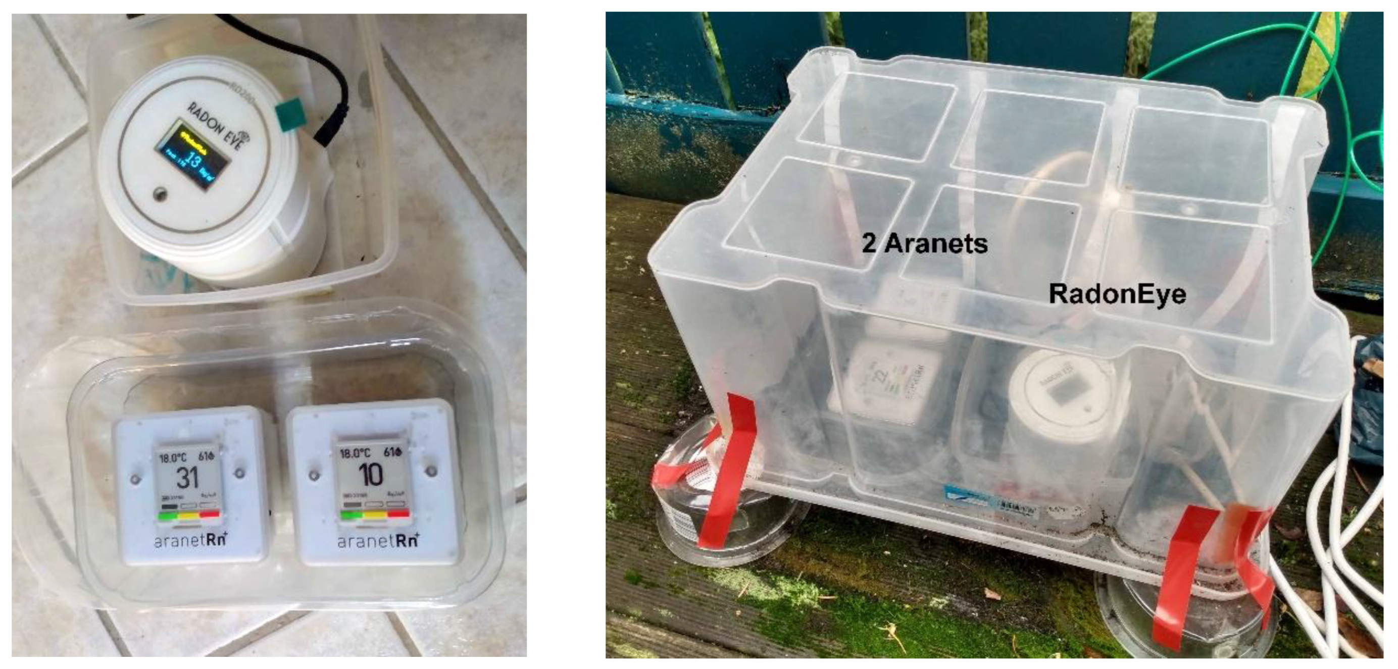
Figure 2.
Aranet monitors on a book shelf and in a staircase.
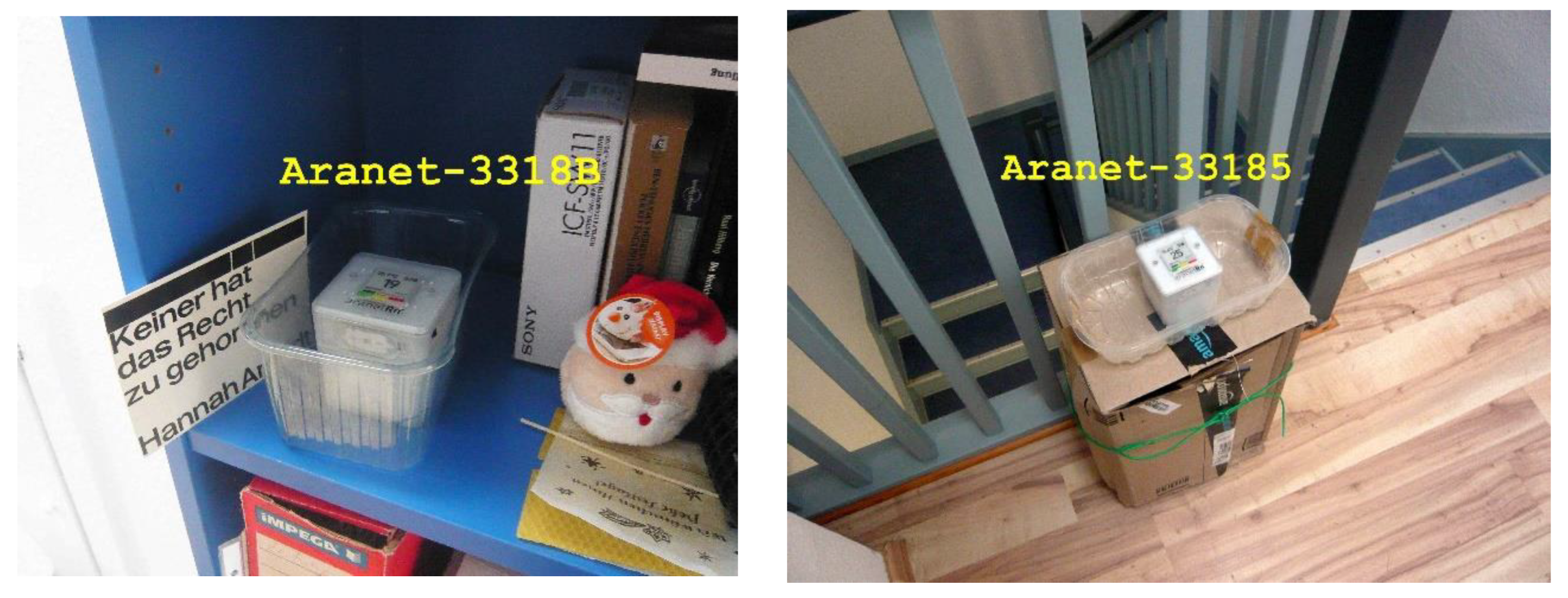
Figure 3.
Exposure to thoron. Left – the plastic container with monazite concentrate; right – the Aranet monitor inserted. On top a Radiacode dose rate monitor (μSv/h). During exposure the container was covered.
Figure 3.
Exposure to thoron. Left – the plastic container with monazite concentrate; right – the Aranet monitor inserted. On top a Radiacode dose rate monitor (μSv/h). During exposure the container was covered.
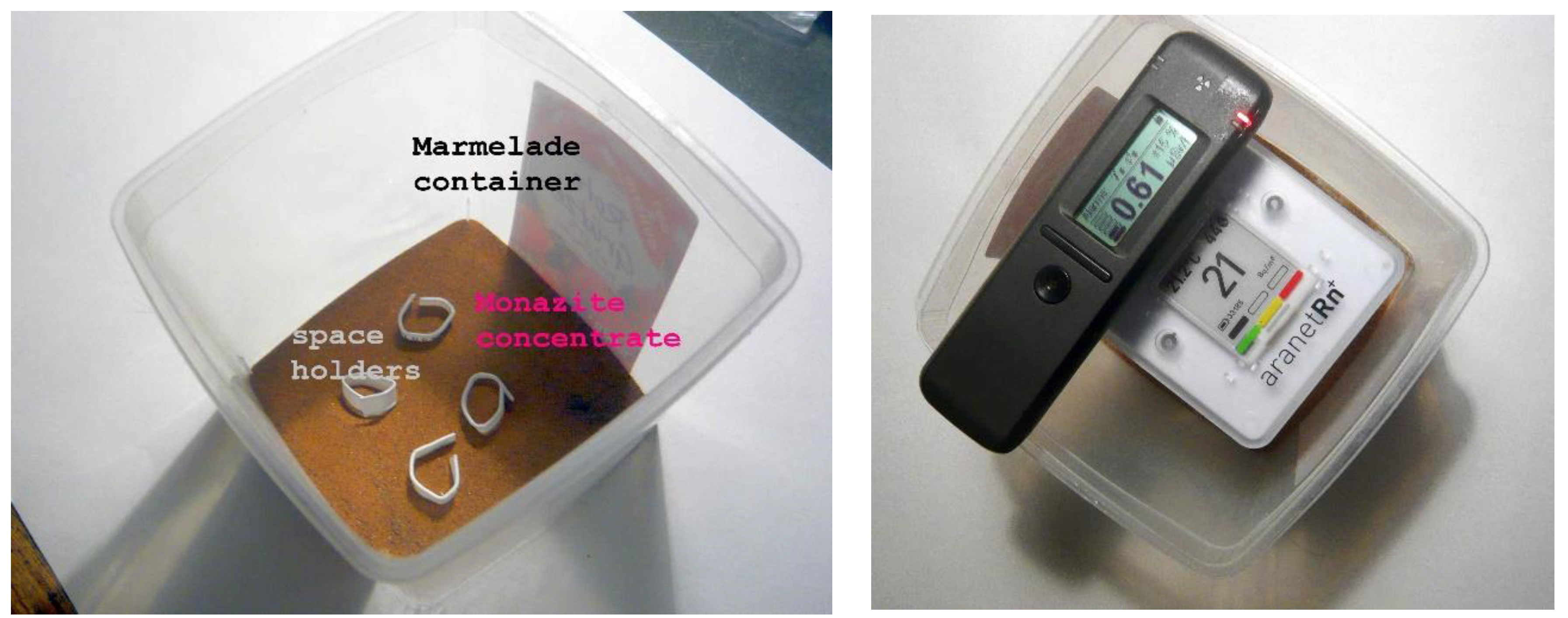
Figure 4.
95% confidence limits assuming Poisson statistic and the nominal sensitivity.
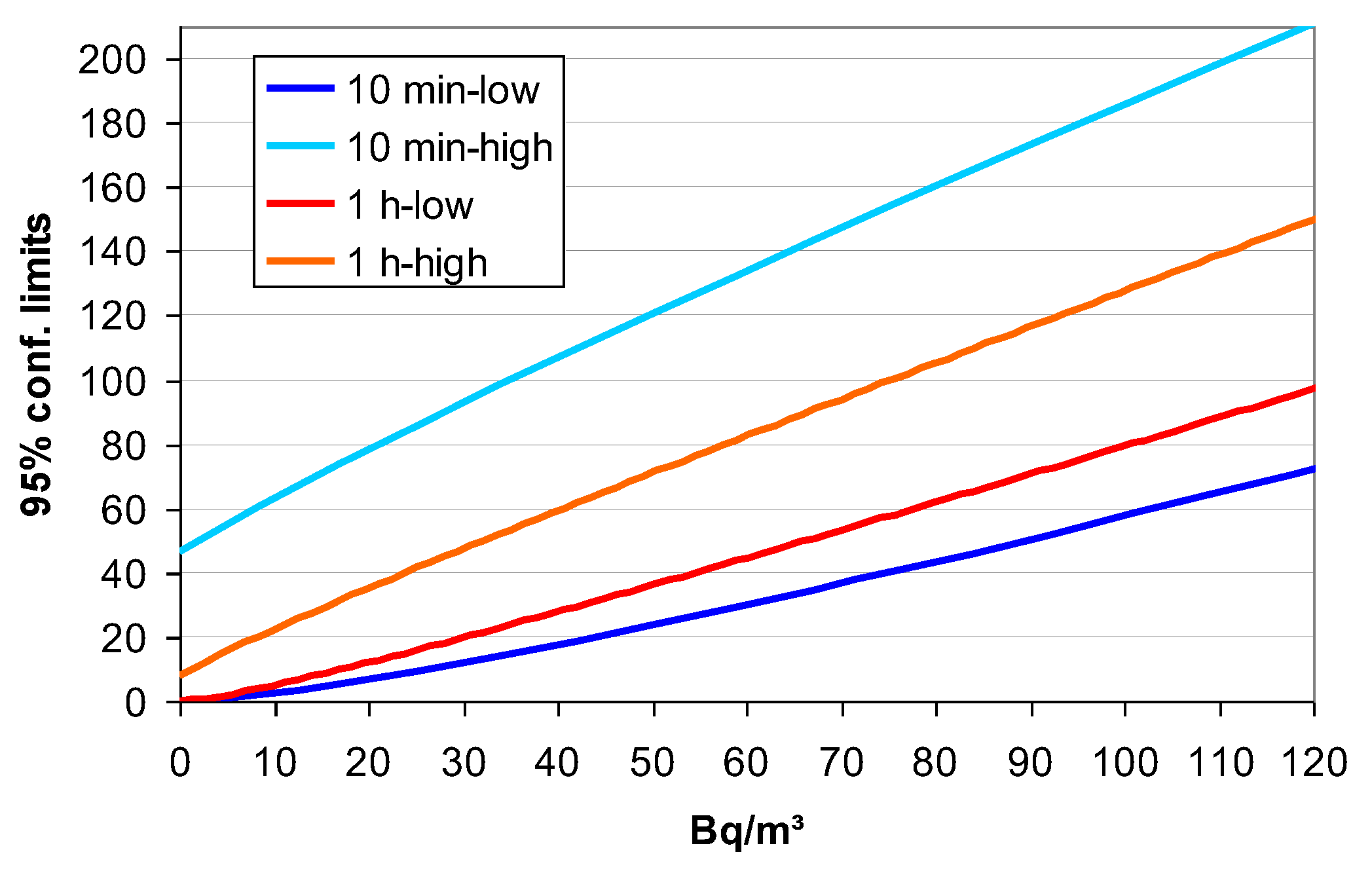
Figure 5.
Decision threshold DT and detection limit LLD.
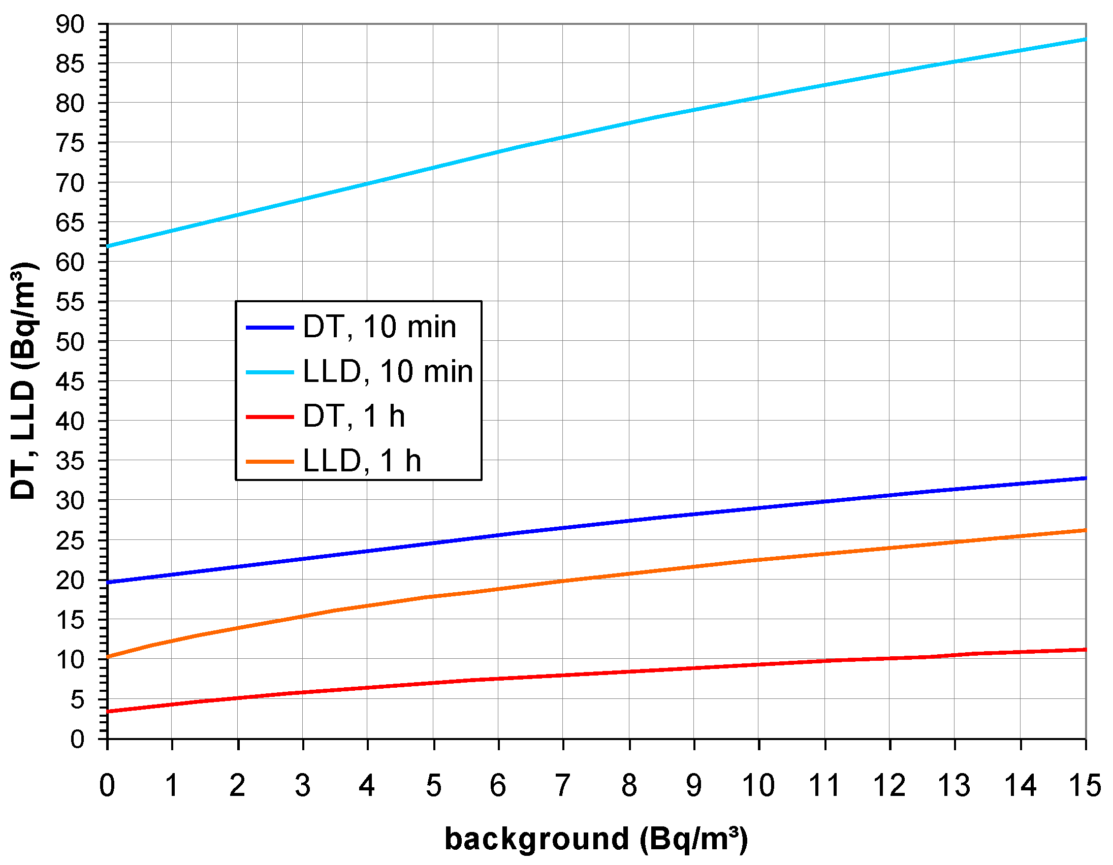
Figure 6.
A transient between 3.11.25 10:00 and about 12:00 caused by moving the monitors from higher (indoor) to lower (outdoor) exposure.
Figure 6.
A transient between 3.11.25 10:00 and about 12:00 caused by moving the monitors from higher (indoor) to lower (outdoor) exposure.
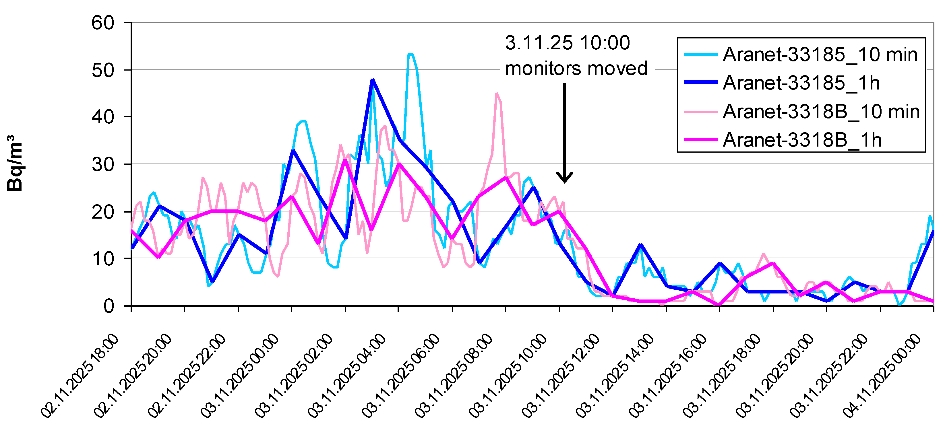
Figure 7.
A transient between 20.11.25 9:45 and about 12:00 caused by moving the monitors from lower (outdoor) to higher (indoor) exposure.
Figure 7.
A transient between 20.11.25 9:45 and about 12:00 caused by moving the monitors from lower (outdoor) to higher (indoor) exposure.
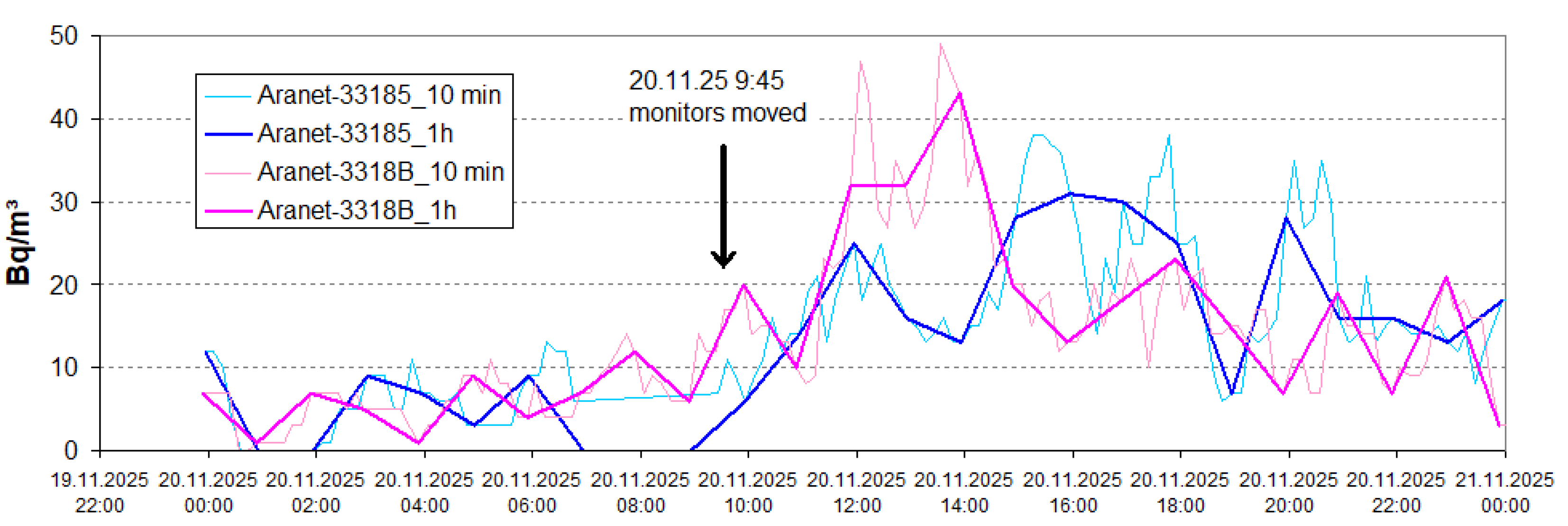
Figure 8.
Radon concentration profile on a journey from Berlin to Vienna. The period between the arrows represents the period when the monitors were exposed essentially to outdoor radon. Note that the data points denote the mean over the preceding hour.
Figure 8.
Radon concentration profile on a journey from Berlin to Vienna. The period between the arrows represents the period when the monitors were exposed essentially to outdoor radon. Note that the data points denote the mean over the preceding hour.
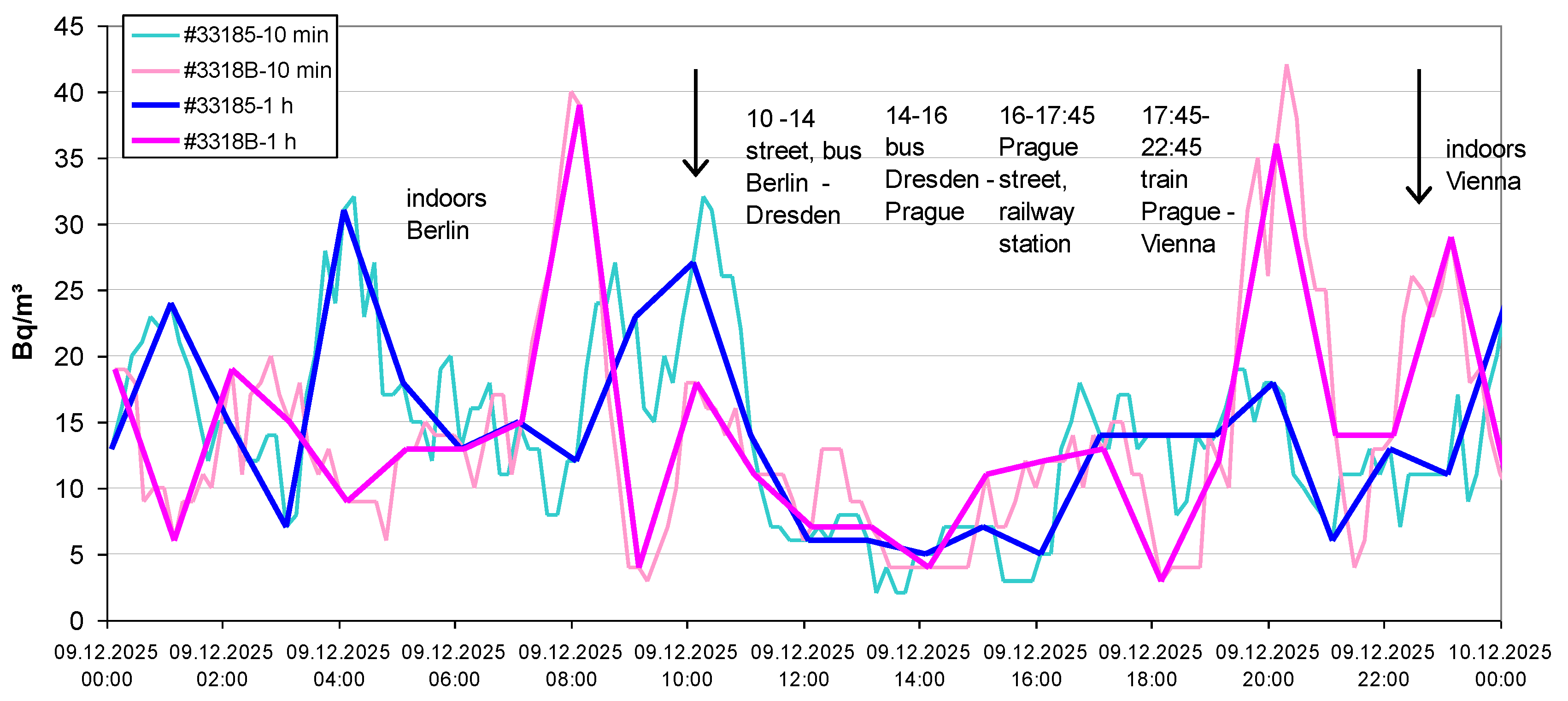
Figure 9.
A spike at ca. 6.11.25 14:00 after the Aranet monitors were moved. Between 4:30 and 13:30 the monitors had stopped recording Rn because of high humidity.
Figure 9.
A spike at ca. 6.11.25 14:00 after the Aranet monitors were moved. Between 4:30 and 13:30 the monitors had stopped recording Rn because of high humidity.
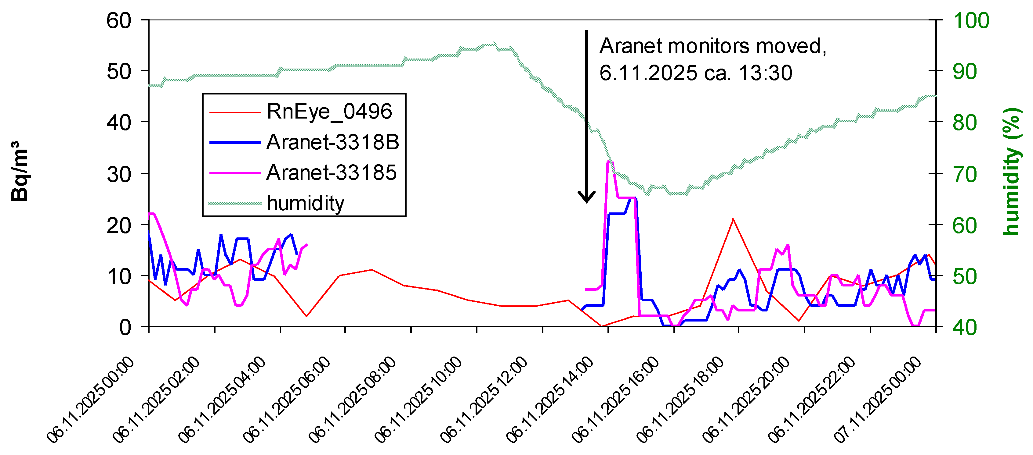
Figure 10.
Four periods of humidity >90% which caused the monitors to suspend recording Rn concentrations.
Figure 10.
Four periods of humidity >90% which caused the monitors to suspend recording Rn concentrations.
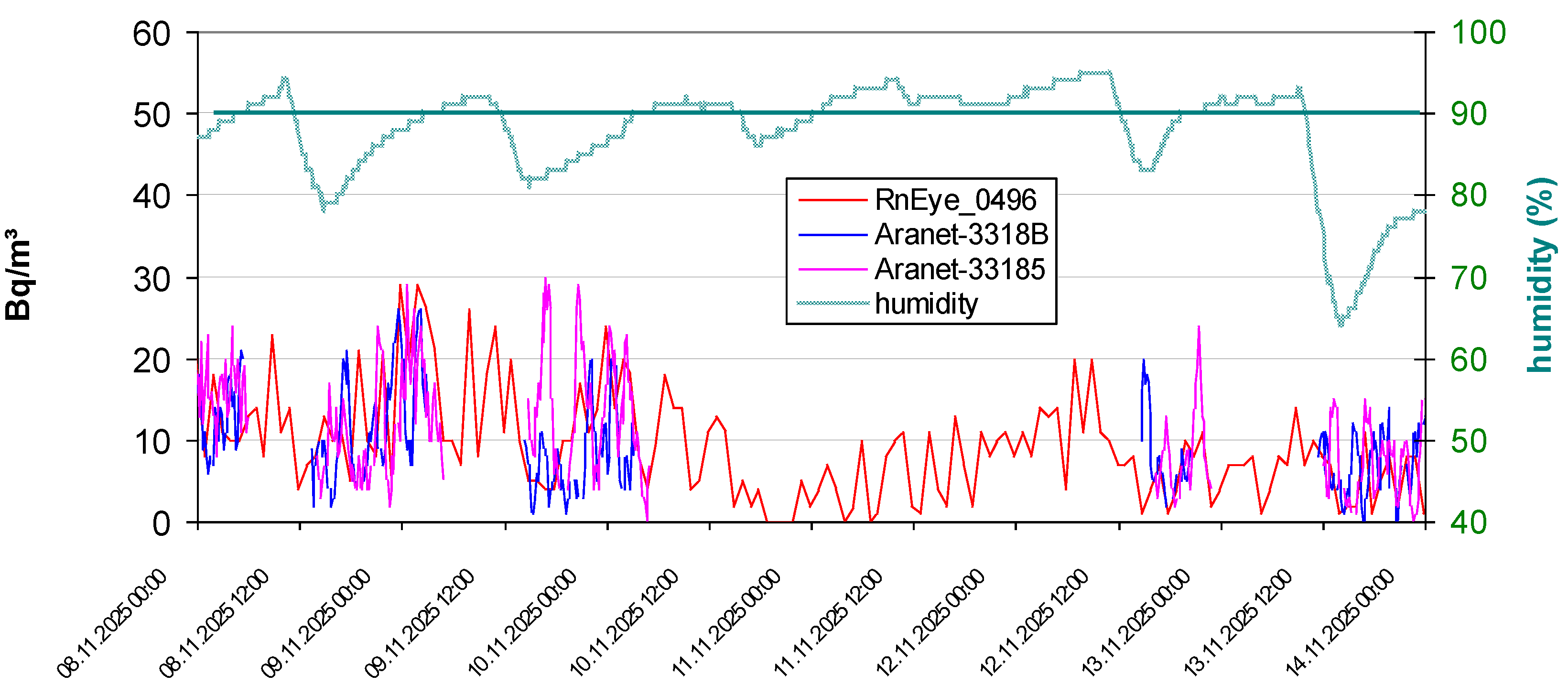
Figure 13.
Parallel measurements of two Aranet and one RadonEye monitor; Berlin indoors.
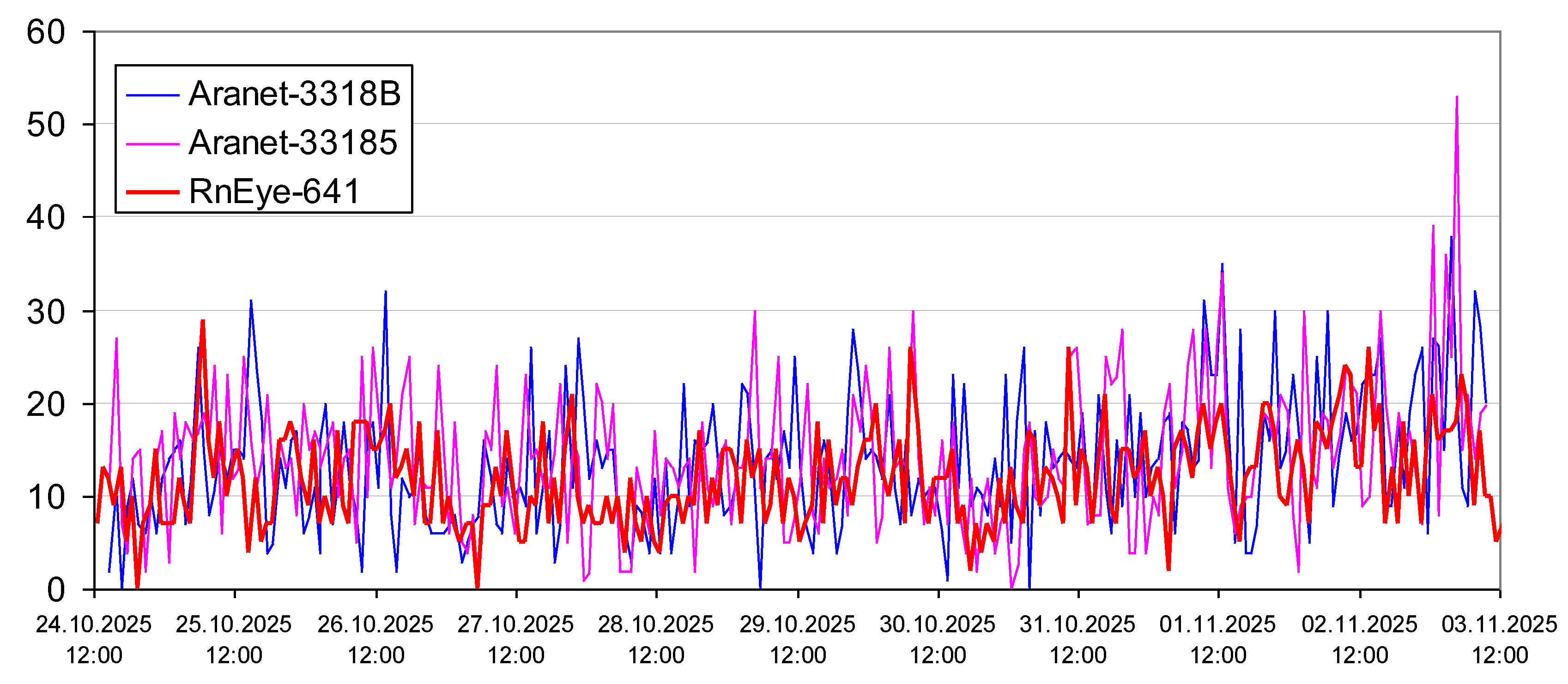
Figure 14.
Parallel measurements of two Aranet and one RadonEye monitor; Berlin outdoors. The gaps in the Aranet series are due to humidity >90% between late night and about noon.
Figure 14.
Parallel measurements of two Aranet and one RadonEye monitor; Berlin outdoors. The gaps in the Aranet series are due to humidity >90% between late night and about noon.
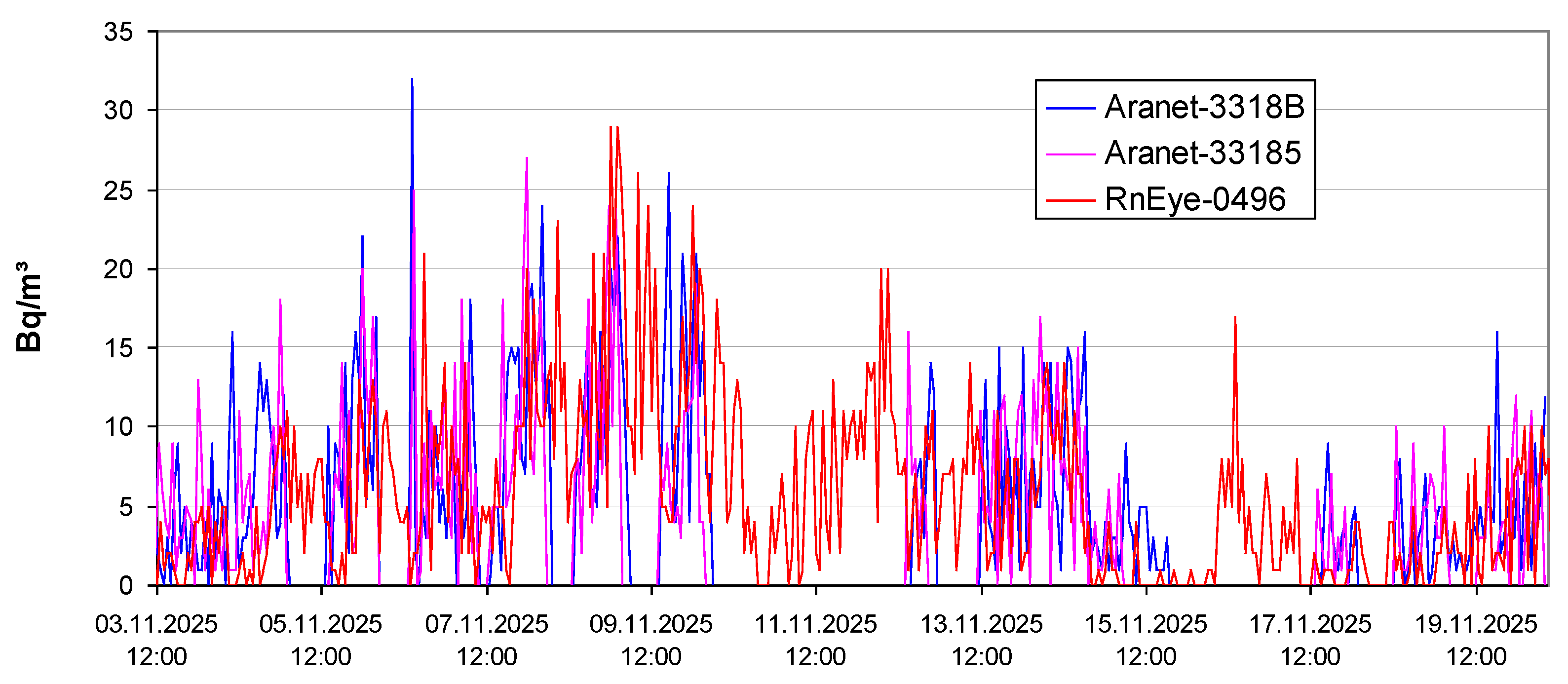
Figure 15.
Radon concentration time series of the three monitors.
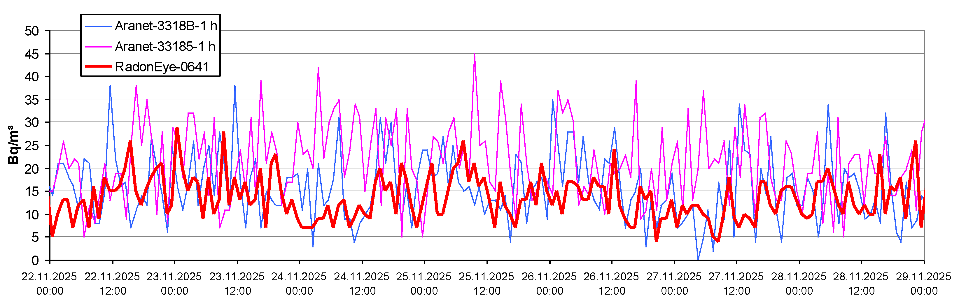
Figure 16.
Thoron exposure: time series of the Aranet readings z; z-BG: estimated background subtracted, 10 minute readings; z-BG – 1h: 1 h-readings.
Figure 16.
Thoron exposure: time series of the Aranet readings z; z-BG: estimated background subtracted, 10 minute readings; z-BG – 1h: 1 h-readings.
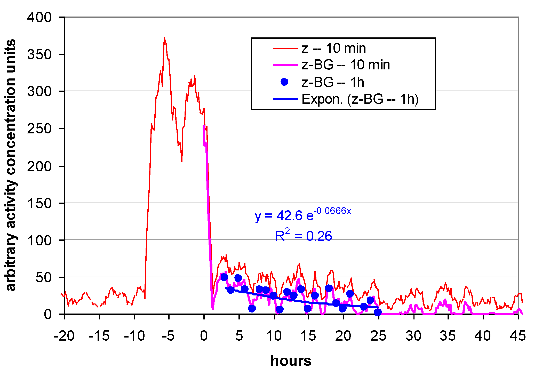
Table 1.
Statistics of counting intervals Δt, Aranet monitors #33185 and #3318B. Units: minutes.
| #33185 | #3318B | |
| AM | 9.9972 | 9.9972 |
| SD | 0.0529 | 0.0529 |
| SE | 0.0014 | 0.0014 |
| n | 1428 | 1428 |
| min | 9 | 9 |
| max | 10 | 10 |
| number(Δt=9) | 4 | 4 |
| Frequency(Δt=9) | 0.0028 | 0.0028 |
Table 6.
Basic statistics of the Rn concentrations measured with three monitors in parallel; Berlin outdoors. AM – arithmetic mean; SD, SE – standard deviation and error; CV – coefficient of variation = SD/AM; n – number of measurements = duration (hours) of the experiment.
Table 6.
Basic statistics of the Rn concentrations measured with three monitors in parallel; Berlin outdoors. AM – arithmetic mean; SD, SE – standard deviation and error; CV – coefficient of variation = SD/AM; n – number of measurements = duration (hours) of the experiment.
| Aranet-3318B | Aranet-33185 | RadonEye-496 | |
| AM (Bq/m³) | 17.6 | 23.4 | 14.7 |
| SD (Bq/m³) | 7.6 | 9.6 | 5.4 |
| SE (Bq/m³) | 0.4 | 0.5 | 0.3 |
| CV | 0.43 | 0.41 | 0.37 |
| n (hours) | 414 | 415 | 417 |
| max (Bq/m³) | 49 | 60 | 32 |
| min (Bq/m³) | 0 | 5 | 4 |
Table 7.
Correlation matrix of the 1 h-values. Lower left triangle: Pearson correlation coefficients; Upper right triangle, italic: p-values. Red: significant, p<0.05.
Table 7.
Correlation matrix of the 1 h-values. Lower left triangle: Pearson correlation coefficients; Upper right triangle, italic: p-values. Red: significant, p<0.05.
| RnEye | #33185 | #3318B | |
| RnEye | 0.2 | 0.0011 | |
| #33185 | 0.062 | 0.13 | |
| #3318B | 0.16 | 0.075 |
Disclaimer/Publisher’s Note: The statements, opinions and data contained in all publications are solely those of the individual author(s) and contributor(s) and not of MDPI and/or the editor(s). MDPI and/or the editor(s) disclaim responsibility for any injury to people or property resulting from any ideas, methods, instructions or products referred to in the content. |
© 2026 by the authors. Licensee MDPI, Basel, Switzerland. This article is an open access article distributed under the terms and conditions of the Creative Commons Attribution (CC BY) license (http://creativecommons.org/licenses/by/4.0/).
Copyright: This open access article is published under a Creative Commons CC BY 4.0 license, which permit the free download, distribution, and reuse, provided that the author and preprint are cited in any reuse.


