
Submitted:
04 January 2026
Posted:
05 January 2026
You are already at the latest version
Abstract
Prior research has consistently shown that students’ SAT scores are influenced by factors beyond academic ability, including socioeconomic background and ethnicity. This study employed aggregated school-level data from Massachusetts and New York City (NYC) to assess the quantitative relationships between average SAT scores and school-level demographics and interventions. The assessment aims to help regional and national education policymakers identify factors related to school academic merits and devise inclusive and effective ways to promote educational equality. Three analytical methods, multiple linear regression, relaxed Least Absolute Shrinkage and Selection Operator (LASSO), and decision trees, were conducted sequentially to decipher the complex relationships among variables. The analysis showed that schools with high percentages of Black, Hispanic, and low-income students tend to have lower average scores than schools with high percentages of White, Asian, and well-off students. Moreover, socioeconomic disadvantage is the most powerful and consistent predictor of lower SAT scores, with race and good academic preparation (i.e., percent attending college) functioning as secondary influences. The results indicate that SAT score disparities reflect structural inequities, and more SAT preparation resources are needed at schools with higher percentages of Black, Hispanic, and low-income students to level the playing field in SAT testing.
Keywords:
SAT
; socioeconomic
; education
; LASSO
; decision tree
1. Introduction
The Scholastic Aptitude Test (SAT) was originally adapted from the Army intelligence quotient (IQ) Test. The first exam, administered in 1926, was used to test applicants to West Point and not for college admission. Grounded in the concept of aptitude, the SAT was designed to predict students’ academic performance by assessing their readiness for college-level work. Unlike tests that evaluate how well a student can perform based on what they have already learned, the original version of the SAT was intended to assess intelligence without the influence of school and family backgrounds. In 1934, James Bryant Conant, the president of Harvard University from the 1930s to the 1950s, referred to the SAT as “Harvard Scholarship Test” and required it for all Harvard applicants in 1941.
Before the SAT, students in American higher education were usually selected based on their families’ economic status. With the SAT, Conant hoped that everyone in America, regardless of their background, would have an equal opportunity to attend college and receive an education. By the late 1930s, the SAT had become a significant component of the admissions process at all Ivy League institutions. Until the 1990s, the SAT was required by most colleges and universities in the United States.
The test-optional movement began in the 2000s, as critics claimed the test was unfair due to score gaps caused by racial and socioeconomic disparities. The movement gained momentum before the pandemic, and the COVID-19 outbreak, which forced colleges to go SAT-optional, created a natural environment for this large-scale experiment. The major policy reports that support this movement, along with the changes made to the SAT testing in response, are shown in Figure 1.
In 2001, the president of the University of California recommended that campuses discontinue using the SAT and adopt assessments more closely aligned with the high school curriculum. The SAT responded in 2005 by increasing testing time, adding a writing section, and removing the word analogies section. Bates College was the first highly selective institution to adopt a test-optional admissions policy in 1984. However, the college has consistently required all enrolled students to submit test scores upon matriculation, enabling institutional research comparing applicants who submitted scores with those who did not. In 2004, Bates presented their 20-year data, showing that the Bates Grade Point Average (GPA) between non-submitters and submitters varied by only 0.05%, despite a 160-point difference in their SAT scores (Hiss and Franks, 2014). Findings from the Bates College study renewed national interest in test-optional admissions policies, prompting a growing number of small, private liberal arts colleges to discontinue standardized testing requirements.
In 2008, the National Association for College Admission Counseling (NACAC) released its Report of the Commission on the Use of Standardized Tests in Undergraduate Admission (NACAC, 2008). The report called on institutions to reconsider the role of standardized test scores in admissions decisions, arguing that SAT scores had limited relevance for course placement, academic advising, and institutional research. NACAC further urged colleges and universities to regularly examine and evaluate the broader implications of standardized testing requirements. These ultimately led many colleges, varying in institutional type and size, to adopt the test-optional movement.
In 2016, the College Board redesigned the SAT by making the essay section optional. In 2021, the essay component was discontinued entirely, reflecting growing concerns about equity, access, and the differential impact of socioeconomic disparities on test performance. When COVID-19 hit in 2020, almost all universities adopted a test-optional policy due to the difficulty of administering tests safely. Following the easing of pandemic-related disruptions in 2023, several highly selective universities, including Harvard University and the Massachusetts Institute of Technology (MIT), reinstated SAT requirements for undergraduate admissions. In 2024, research from Opportunity Insights, a team of Harvard-based researchers and policy analysts, suggested that SAT scores are more predictive of post-college success than high school grades (Chetty et al., 2023). In the same year, the SAT exam was converted to its current digital format and reduced from three hours to approximately two hours.
The proponents of the test-optional policy criticized the tests as unfair because emerging debates suggest that non-academic factors, including socioeconomic status and ethnicity, significantly influence these scores. Average scores for students from modest-income backgrounds, as well as those who are Black or Hispanic, are lower than those for white, Asian, and upper-income students. These critics worry that reinstating test requirements will reduce diversity in college admissions. In theory, the creation of the SAT was intended to provide equal opportunities for all students, regardless of their background. However, the SAT is now alleged to create inequalities among applicants, contradicting the rationale behind its creation. This shift raises an important question: how did an assessment once viewed as an educational “equalizer” come to be regarded as a symbol of inequality in later decades? This also raises an interesting research question: Are socioeconomic disparities primary drivers of SAT score performance, or is the SAT merely a reflection of the inherent inequities in the education system?
The current study is predicated on the hypothesis that SAT scores are not merely reflections of academic intelligence but are also shaped by many external factors. It employed aggregated school-level data and examined the quantitative effects of student body composition (race/ethnicity and economic disadvantage), college attendance, and school funding levels on their average SAT performance. Traditional multiple linear regression and machine learning methods (relaxed least absolute shrinkage and selection operator (LASSO) and decision tree) were used in the analysis to unravel the intricate web of elements influencing SAT scores. This analysis aims to help regional and national education policymakers identify factors related to school academic merits and devise inclusive and effective ways to promote educational equality and quality (Liu et al., 2024).
2. Related Work
The Coleman Report, titled “Equality of Educational Opportunity,” is a landmark study that analyzes the factors contributing to educational achievement (Coleman, 1966). The report found that family background (especially parental education and income) was a stronger predictor of student performance than school facilities or resources. Since then, a growing body of literature across disciplines has explored the relationship between income and academic achievement. However, research on the relationship between family background (e.g., income, race/ethnicity) and SAT performance began to surge in the 2000s, concurrent with the test-optional movement. A list of previous studies on the relationship between family background and SAT performance is shown in Appendix 1, and their key findings are summarized below.
In 2001, the president of the University of California (UC) urged institutions to reconsider the use of the SAT, arguing that it did not adequately reflect the high school curricula at many schools. Studies conducted on over 1.6 million California high school graduates who applied to the UC system between 1994 and 2016 confirmed that SAT/ACT scores are most significantly influenced by family background, including low-income status, first-generation college attendance, and minority status (Geiser, 2017), (Geiser, 2020). Geiser’s analysis further demonstrated that race/ethnicity exerts an independent statistical effect on SAT/ACT scores, even after controlling family income and parental education (Geiser, 2015).
Studies conducted by the College Board have consistently documented a positive association between socioeconomic status (SES) and SAT scores. The results from Camara and Schmidt indicated that parental income and education are strongly related to performance on various measures, with parental education showing the stronger relationship (Camara and Schmidt, 1999). However, they argued that (1) parental income and education are closely related to many other predictors and outcomes of academic performance, including high school GPA and class rank; and (2) Hispanic and African American students from comparable socioeconomic backgrounds tend to score lower than their Asian American and White peers. Results from Sackett at 41 colleges and universities from 1995 to 1997 and at 110 colleges and universities in 2006 confirmed that students from higher-income backgrounds generally achieve higher scores (Sackett et al., 2009a), (Sackett et al., 2009b). However, the researchers also found that standardized test scores predict subsequent academic performance in colleges and universities, independent of socioeconomic status (SES). They suggested that the observed relationship between SAT scores and SES likely reflects a combination of educational opportunities, school quality, peer effects, and other social factors (Sackett et al., 2012).
Studies by Zwick examining the relationship between socioeconomic status (SES) and various academic outcomes and performance indicators have shown that SAT scores exhibit more minor associations with SES than other measures, such as high school grades and class rank (Zwick and Green, 2007), (Zwick and Himelfarb, 2011).
An analysis by Dixon-Roman from a large dataset (781,437 Black and White college-bound high school students who took the SAT in 2003) suggested a strong correlation between SAT scores and socioeconomic background, including household income. Empirical evidence indicates that students from higher-income families tend to earn higher SAT scores than their lower-income peers, with income-related score disparities being substantially larger among Black students than among White students (Dixon-Román, 2013). Studies published in The Journal of Blacks in Higher Education similarly documented a persistent Black-White SAT performance gap. They demonstrated that measures of family economic background capture part of this disparity. However, these analyses also argued that differences in family income alone do not fully account for racial and ethnic disparities in overall SAT scores (JBHE, 1998a; JBHE, 1998b). A 2004 study suggested that differences in school quality may be a significant factor in the explanation (Fryer and Levitt, 2004).
One study by Kobrin employed hierarchical linear modeling (HLM) to investigate student- and school-level predictors of the score discrepancy, identifying school-level factors such as economic advantage and school size as significant predictors of a school’s average discrepancy score (Kobrin et al., 2003). Everson and Millsap examined both individual- and school-level contributions to SAT score gaps using multilevel latent variable modeling techniques. Their results indicated that, after accounting for school-level effects, the SAT performance gaps between different socioeconomic classes were reduced by an average of 50 points (Everson and Millsap, 2004). These findings suggest substantial disparities in the distribution of educational resources across schools, which in turn contribute to differences in SAT scores.
We found that most existing studies have focused on individuals’ family backgrounds without accounting for the school environment in their analyses. The school-level factors, such as students’ accessibility to quality education, higher education culture, and school funding, and their impact on SAT scores, are rarely discussed. More importantly, the well-known multicollinearity and interaction effects among socioeconomic factors were, for the most part, not thoroughly examined.
Thus, there remains a need for closer investigation of the family and school effects on SAT performance using modeling methods that can untangle the interactions among factors in feature selection and predict the quantitative response to a chosen condition. As a result, in this study, we aimed to develop a well-specified model of the relationships between family and school-level factors and their unique and joint influences on the school’s SAT performance.
3. Method
The study utilized two SAT score datasets on Kaggle.com: Massachusetts (MA) Public Schools Data and Average SAT Scores for New York City (NYC) Public Schools. The Massachusetts dataset includes student body (demographic distributions such as percentage of gender, ethnicity, economic situation), funding levels (class size, Per Pupil Expenditure), college attendance, and testing (SAT, MCAS, APs), and was compiled from the data in the Massachusetts Department of Education reports in 2017. The NYC dataset includes student races, neighborhoods, and average SAT scores for the 2014-2015 school year. Also, in this study, we use R (R Core Team, 2024), version 4.4.1, for data processing, visualization, and model-based analysis of the actual and predicted data.
An Ontology heatmap comparing population distribution by race across all 50 states was produced, which justifies our comparison between MA and NYC, as illustrated in Figure 2. Based on the heatmap, states with population distributions like MA’s included Illinois, Connecticut, Colorado, Kansas, Arkansas, Alaska, Kentucky, Iowa, Indiana, and Idaho, suggesting we could generalize our MA predictions to these states. To further expand our analysis, we sought to explore a state with different population demographics than MA. As seen on the ontology map, New York had a drastically different population. To make data easier to find, we focused solely on NYC.
Data processing steps below were used to construct the analytical dataset for MA:
- Removed data from elementary, middle schools due to a lack of SAT scores.
- Removed irrelevant outcome variables (i.e., AP scores) as the analysis focused solely on SAT scores
- Renamed variables for operational simplicity
- Converted old SAT score (out of 2400) to new SAT score (out of 1600)
- Mutated the percentages to numbers for ease of computing.
For the NYC dataset, we selected only race variables for analysis, removing other variables such as the percentage of students who took the test and school size. However, we kept these variables for data visualization. The NYC dataset did not contain the same variables as the Massachusetts dataset.
3.1. Data Visualization
Data visualization tools, such as histograms, box plots, and heatmap analysis, were used to identify central tendencies and outliers in both datasets. First, we produced histograms of SAT scores in MA and NYC, as illustrated in Figure 3 and Figure 4. The mean SAT score for MA was around 1000, and the curve was bell-shaped, indicating a normal distribution. The mean SAT score in NYC was around 750; the curve was slightly right-skewed.
For the MA dataset, additional school features, including average in-district expenditures per pupil, the percentage of economically disadvantaged students, and the percentage of people attending college, were also visualized in a histogram (Figure 3). The histogram showing expenditure per pupil at each school was skewed to the right with a mean expenditure around $13000 and a noticeable outlier just before $20000; The percentage of students economically disadvantaged was skewed right, meaning most schools had low mean percentage of eco-nomically disadvantaged students, around 10%; the percentage of people attending college was skewed to the right, indicating most schools had a high rate of students attending college, a mean of around 90%.
For the NYC dataset, histograms were also produced for the student enrollment and the percentage of students at the school who took the SAT (Figure 4). Student enrollment was skewed to the right, with a mean of around 500 per school. The percentage tested per school followed a relatively normal distribution, with the mean around 60%. Directly comparing the NYC data to the MA data, the mean SAT score for MA is noticeably higher (1000 vs. 700). While the other data visualizations cannot be directly compared, they provide a good context for the state/region.
Furthermore, boxplots were generated to compare race percentages across schools in MA and NYC. As shown in Figure 5, MA schools generally have higher percentages of Caucasians than African Americans, Asians, and Hispanics (Figure 5). Conversely, in New York City, the percentages of Hispanics and African Americans are significantly higher than those of Caucasians and Asians (Figure 6).
As shown in the MA correlogram (Figure 7), the percentage of economically disadvantaged individuals had a large positive correlation with the percentages of African Americans and Hispanics. This correlogram was not generated for the NYC dataset, as it only contained races.
3.2. Model-Based Analysis
Three analytical methods, multiple linear regression (MLR), relaxed Least Absolute Shrinkage and Selection Operator (LASSO), and decision trees, were conducted sequentially to decipher the complex relationships among variables. By combining these three methods, we leverage their complementary strengths. MLR provides a statistically interpretable baseline, while relaxed LASSO refines the model by selecting the most influential factors, accounting for multicollinearity. Decision trees, on the other hand, explore non-linear interactions to capture the complexity of school environments. Together, they provide a robust, multi-perspective analysis of the socioeconomic and demographic factors shaping SAT outcomes.
3.2.1. Multiple Linear Regression (MLR)
MLR is especially useful for estimating the relationship between a single dependent variable (average SAT score) and multiple independent variables (such as race percentages). The coefficients it produces quantify how much the dependent variable is expected to change when the independent variable increases by 1 unit, while holding all other variables constant. We used this analysis first because it provides an interpretable baseline model that indicates the direction and magnitude of correlation. It also enables us to test for statistical significance and identify which predictors have a meaningful relationship with SAT scores. We used backward selection for the model, retaining only statistically significant predictors at the 0.001 level.
To validate our MLR assumptions, we used the plot function to create a Residual vs. Fitted plot and a normality QQ plot to assess homoscedasticity and linearity. For both MA and NYC, the Residual vs. Fitted plot showed an equal distribution of points above and below the line, indicating homoscedasticity. Our Normality QQplot demonstrated a linear relationship, indicating linearity (Figure 8 and Figure 9).
Additionally, for each coefficient in the multiple linear regression model, we calculated a 95% confidence interval to quantify the uncertainty of the estimated effect. This allowed us to assess the magnitude and reliability of each predictor’s impact on SAT scores. Since none of the intervals include zero, this indicates the relationship between all the predictors and the SAT score is statistically significant.
3.2.2. Relaxed LASSO
Since regression models are sensitive to multicollinearity, it is common for demographic variables (e.g., race and economic disadvantages) to overlap. To address this, we used the Relaxed LASSO analytical method. Instead of keeping all correlated variables, it picks one variable from a correlated group, reducing overfitting. The relaxed LASSO also moves less relevant predictors towards zero and refits the model with less shrinkage on the selected variables. While MLR outputs effect sizes, relaxed LASSO produces a more parsimonious model.
To visualize our relaxed LASSO model, we generated a cross-validation plot showing how predictive error changes across different levels of penalization, represented by the penalty parameter λ (plotted as −log(λ)) (Figure 10 and Figure 11). The x-axis represents the strength of the penalty, with larger values corresponding to more substantial shrinkage. At the same time, the y-axis shows the cross-validated prediction error, measured as mean squared error. This plot illustrates how the model’s complexity varies with λ: larger values produce simpler models with more coefficients shrunk to zero, whereas smaller values produce more complex models with more variables retained. For the MA dataset, the model with the minimum error included 9 variables, while for the NYC dataset, the minimum-error model included 4 variables.
3.2.3. Decision Tree
We also used a decision tree, a non-linear Machine Learning model that separates data into subgroups based on predictor values. At each node, the algorithm evaluates all candidate predictors. It identifies the variable and threshold that minimizes the prediction error (measured by metrics such as residual sum of squares for regression trees). The selected split produces two child nodes that are more homogeneous with respect to the response variable than the parent node. This process continues iteratively, generating a tree structure composed of decision rules of the form “if condition A, then outcome B.” Unlike regression models, which assume a linear relationship between predictors and the outcome variable, decision trees capture nonlinearities and interaction effects. For example, in this study, the algorithm may first split schools by the percentage of economically disadvantaged students, then further separate each branch by demographic or college attendance rates. Notably, the same predictor can be used at multiple nodes, each with a different threshold, allowing the tree to model complex relationships across the range of variables. For both the MA and NYC datasets, the decision tree generated graphical tree diagrams, where each split corresponded to a demographic or socio-economic factor, and each terminal node provided a predicted average SAT score for schools within that subgroup. This approach offers interpretable “if–then” rules for predicting school-level SAT scores, highlighting the most influential factors in shaping score disparities. The decision tree provides a straightforward, interpretable approach to predicting a school’s SAT score from its demographic factors, making it a practical, intuitive tool for policymakers.
4. Results
4.1. Multiple Linear Regression
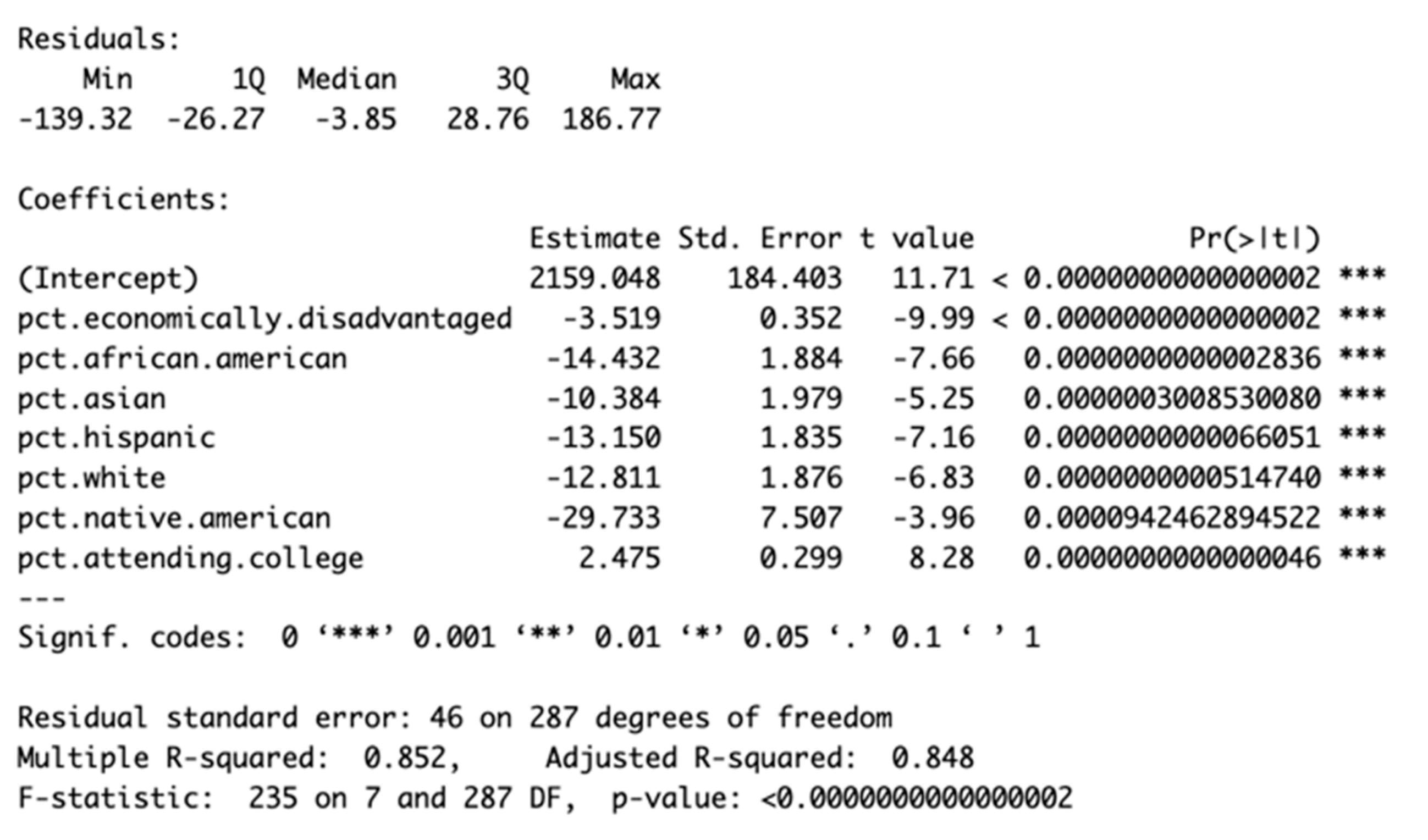
We used multiple linear regression on both the MA and NYC datasets. For MA data, the model (Equation 1) demonstrated that the percent of economically disadvantaged students, the percent of students from racial groups (i.e., Asian, Hispanic, African American, White, Native American), and the percent of college matriculation were significant at the 0.001 level.
Equation 1 (MA)
Furthermore, the R-squared value was 0.85, indicating a relatively high correlation between the variables and the average SAT score. The percentages of economically disadvantaged individuals and of individuals from all racial groups showed negative correlations with the SAT score. A 1% increase in the percentage of low-income students would result in a decrease of 3.5 points in the school’s average SAT score. The percentage of Asians had the least negative correlation, whereas the percentage of Native Americans had the most significant negative correlation. A 1% increase in the percentage of Asian or Native American students would lead to decreases of 10.4 points and 29.73 points in the school’s average SAT score, respectively. The percentage of students attending college had a positive correlation. A 1% increase in the percentage of students attending college at a school would increase 2.5 points in the school’s average SAT score.
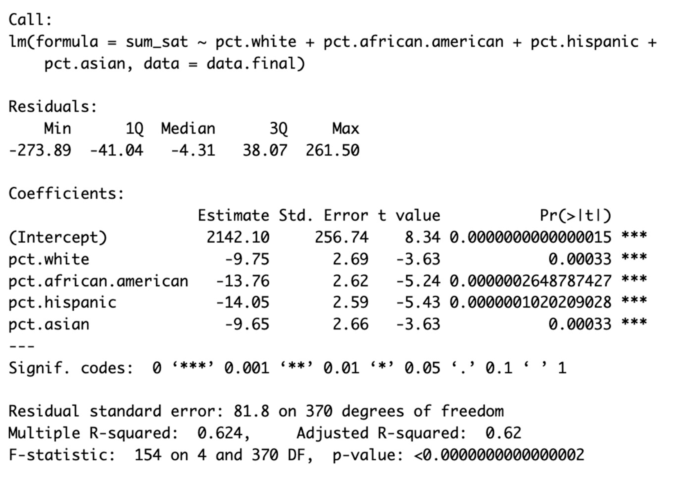
For the NYC dataset, the initial MLR (Equation 2) showed that all variables were statistically significant at the 0.001 level.
These variables included the percentage of students from specific racial groups (e.g., White, African American, Hispanic, Asian). Thus, no backwards selection was needed. All races were negatively correlated with SAT scores, with the percentage of Hispanic students showing the highest negative correlation and the percentage of Asian students showing the lowest. A 1% increase in the rate of Asian or Hispanic students would lead to decreases of 9.7 points and 14.1 points in the school’s average SAT score, respectively.
MA and NYC showed similar patterns of correlation, with all racial groups exhibiting negative correlations with SAT scores. Asians always had the lowest negative correlation, and historically excluded minorities such as Hispanics and Native Americans had higher negative correlations. Both MLR models have an abnormally high intercept, 2159 and 2142, respectively. Both numbers are above the maximum SAT score of 1600. An explanation for this phenomenon is that our data does not include 0% values, as no schools have a 0% percentage. Thus, the intercept is extrapolating beyond the observed data, resulting in a significant value.
4.2. LASSO Results
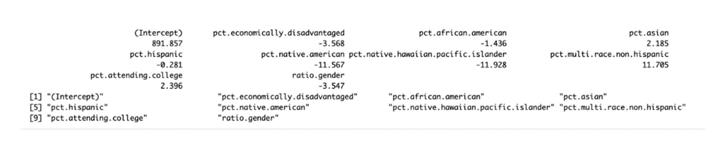
As shown in Table 1, the relaxed LASSO regression selected nine significant factors correlated to SAT score in MA: Percent of economically disadvantaged students, the percent of students of certain races (i.e., Asian, Hispanic, African American, White, Native American, Native Hawaiian Pacific Islander, Multi-race), and the gender ratio of boys to girls. All races were negatively correlated to SAT scores, except for the percent of Asians and Multiracial. The percentage attending college was positively correlated, while the percentage of economically disadvantaged individuals was negatively correlated. A 1% increase in the rate of Asian or multiracial students would lead to a 2.2-point and 11.7-point increase in the school’s average SAT score, respectively. In contrast, a 1% increase in the percentage of Native Hawaiian and Pacific Islander students would lead to a 11.9-point decrease in the school’s average SAT score. Additionally, a 1% increase in the college attendance rate would result in a 2.4-point increase in SAT scores. In contrast, a 1% increase in the percentage of economically disadvantaged students would lead to a 3.6-point decrease in the average SAT score.
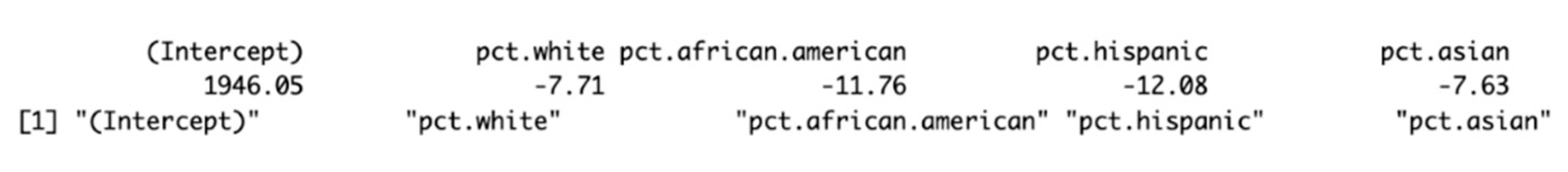
For the NYC dataset, the relaxed LASSO selected all four race variables (Table 1). All race variables were negatively correlated with SAT scores, with the percentage of Asians showing the least negative correlation and the percentage of Hispanics showing the most negative correlation. A 1% increase in the rate of Asian or Hispanic students would lead to decreases of 7.6 points and 12.1 points in the school’s average SAT score, respectively.
4.3. Decision Tree Analysis
In Massachusetts, the decision tree analysis further illuminated the hierarchical structure of factors influencing school-level SAT performance (Figure 12). The first and most important split was on the percentage of economically disadvantaged students, indicating that socioeconomic status is the strongest predictor of SAT outcomes. Schools with ≥ 35.5% economically disadvantaged students consistently had lower average SAT scores, while those with lower proportions performed more competitively. Within the high-poverty group, further splits occurred on % economically disadvantaged (at 59.2%) and subsequently on % Hispanic (at 31.6%). This indicates that, among schools already serving predominantly low-income populations, racial composition has additional influence; schools with higher percentages of Hispanic students had lower SAT scores.
For schools with < 35.5% disadvantaged students, the next major split was again on % economically disadvantaged (at 11.8%), highlighting that even moderate differences in poverty levels create meaningful score gaps. Within this branch, splits on college matriculation rates (65.8% and 89%) revealed that schools sending higher proportions of graduates to college have higher SAT averages.
At schools with < 11.8% disadvantaged, the model split on % Asian students (at 9.3%), suggesting that at schools with more well-off students, racial composition has a positive effect on SAT scores. Schools with higher percentages of Asian students had the highest predicted average SAT scores in the dataset.
This MA decision tree highlights three main findings. First, economic disadvantage is the dominant predictor of SAT score, appearing repeatedly at multiple thresholds. Second, race functions as a secondary, conditional factor. For example, the percentage of Hispanic students is influential within high-poverty schools, while the percentage of Asian students is influential within low-poverty schools. Third, school culture, as defined by college attendance rates, is a strong positive predictor in schools with a moderate proportion of low-income students. Together, these patterns indicate that a student’s economic status at a school account for the majority of score disparities, while race and college-going culture refine the outcomes.
The decision tree for NYC was based solely on racial composition (Figure 13). The first split was based on the percentage of White individuals (14.8%), suggesting that the White demographic is the most important predictor of SAT scores. Schools with fewer than 14.8% White students generally scored lower, while schools with a higher percentage of White students performed better.
Within the low-White branch (<14.8%), the tree is further split by percent Asian (18.8%). Schools with very low Asian representation (< 2.5%) scored the lowest overall, while those with moderate Asian representation (≥ 2.5%) performed better, especially when combined with low Hispanic enrollment (< 9.1%).
Within the high-White branch (≥ 14.8%), the model next split on the percentage of Hispanic individuals (18.9%). Schools with higher Hispanic enrollment scores tended to score lower, while those with lower Hispanic enrollment scores tended to score higher. Among schools with lower Hispanic enrollment, the final split was again based on the percentage of White students (26.2%), with higher White representation associated with the highest predicted SAT averages.
Although the NYC decision tree produced clear splits by racial composition (percentage of Whites, Hispanics, and Asians), these results should be interpreted cautiously. Unlike the Massachusetts dataset, the NYC dataset lacked socioeconomic and cultural variables, such as the percent economically disadvantaged and the percent attending college. So, although the NYC decision tree reflects racial patterns, it’s less informative.
5. Discussion
From our study, we observed a strong correlation between schools’ average SAT scores, the socioeconomic status distributions of school students (e.g., percentage of economically disadvantaged students), the percentage of students from a particular racial background, and schools’ academic preparation (e.g., percentage of students attending college). Further Heat Map Analysis was conducted for Massachusetts to test the conclusions from the LASSO and MLR models. Counties with a higher percentage of economically disadvantages had a lower average SAT score. For instance, Hamden County represents this fact. The analysis also revealed that schools with low SAT performance tend to have low school expenditure per student - nearly all other counties exhibit this trend, except for Boston (Figure 14).
Despite the high correlation between the percentage of students with economic disadvantages and the percentage of African American and Hispanic students, all three variables were selected using the LASSO approach and showed a negative correlation with SAT scores. Race had smaller coefficient estimates than economic disadvantage. The results indicate that race negatively contributed to score discrepancy, independent of economic disadvantages, but it has a weaker influence. The results from decision tree-based modeling further confirmed that economic disadvantage is the strongest predictor of SAT scores, compared to race and college attendance rates.
We conducted the analysis from two regions in the U.S. with distinct racial distributions. The results concerning race factors are consistent with one another: schools with higher per-centages of White and Asian students have higher average SAT scores than schools with higher percentages of African American and Hispanic students. Future work should expand the scope of analysis to additional states and regions, incorporating more comprehensive variables.
Further refinement of machine learning approaches could also better capture nonlinear interactions and more clearly explore causality. Ultimately, the long-term goal is not only to understand disparities but also to provide policymakers with actionable tools, such as apps or websites, to guide the equitable allocation of educational resources.
6. Conclusions
This study analyzes the socioeconomic and demographic drivers of SAT performance using school-level data from Massachusetts and New York City. We applied multiple linear regression, relaxed LASSO, and decision trees as complementary analytical tools. Across all three methods, a consistent theme emerged: economic disadvantage is the most potent predictor of SAT outcomes in MA. Race and academic preparation (i.e., the percentage of students going to college) had additional secondary influences, often conditional on the proportion of economically disadvantaged students. Schools with high percentages of Black, Hispanic, and low-income students tend to have lower average scores than schools with high percentages of White, Asian, and well-off students. Although a correlation is apparent, there is no evidence of causality, highlighting that the SAT reflects and amplifies inequities already embedded in the education system. These results align with prior research [20], while providing new insights by highlighting the interaction between economic and racial factors at the school level. The results indicate that more SAT preparation resources are needed at schools with higher percentages of Black, Hispanic, and low-income students to level the playing field in SAT testing.
Appendix A
List of Prior Studies to Examine Individual and School-Level Effects on SAT Score Gaps
| Year | Author | Report Title (shortened) | Source Data | Method | Data Type |
| 2017; 2020 | Geiser | Norm-referenced tests and race-blind admissions | 1.1 million California high school graduates who applied for freshman admission at UC from 1994 through 2011; and new data for the years 2012 to 2016 (total 1.6 million) | Regression model | Individual data |
| 1999 | Camara | Group Differences in Standardized Testing and Social Stratification | 1,127,021 of college-bound seniors completed the SAT I in 1997 | Descriptive statistics | Individual data |
| 2009; 2012 |
Sackett | Socioeconomic Status and the Relationship Between the STA and Freshman GPA | 136,725 students at 41 colleges and universities from 1995-1997 (2009); 143,606 students at 110 colleges and universities in 2006 (2012) | Regression model | Individual data |
| 2013 | Dixon-Roman | Race, Poverty and SAT Scores | 781,437 Black and White college-bound high school seniors who took the SAT in 2003 | structural equation model (SEM) | Individual data |
| 2007; 2011 | Zwick | New Perspectives on the Correlation of SAT Scores, High School Grades, and Socioeconomic Factors |
a 25% random sample of the 2004 “College bound Seniors” consisted of 336,216 students from a total of 15,768 high schools | Linear regression models | Individual data |
| 1998; 2006 |
The Journal of Blacks in Higher Education | Understanding the black and white test score gap | College board report | Descriptive statistics | Aggregated data |
| 2003 | Kobrin | An Investigation of School-Level Factors for Students with Discrepant High School GPA and SAT Scores. | 18,674 college-bound seniors from 949 high schools from a college board dataset | hierarchical linear model | Individual and aggregated data |
| 2004 | Everson | Beyond Individual Differences: Exploring School Effects on SAT Scores |
1,14 million students completed the SAT in 1995 | multilevel structural equation model | Individual and aggregated data |
Appendix B
Documentation for MLR Equation 1 (MA Data) and Equation 2 (NYC Data)
B.1. Massachusetts
B.2. NYC
Appendix C
Documentation for Table 1
C.1. Massachusetts
C.2. NYC
Appendix D
Positive and Negative Correlation Factors Using MLR and LASSO
| Methods | Massachusetts | NYC | |
| Positive correlations | Negative correlations | Negative correlations | |
| MLR | Percent Attending College | Percent Native American Percent African American Percent Hispanic Percent white Percent Asian Percent economically disadvantaged |
Percent Hispanic Percent African American Percent white Percent Asian |
| LASSO | Percent multi race non-Hispanic Percent Attending College Percent Asia |
Percent Pacific Islander Percent Native American Percent economically disadvantaged Percent African American Percent Hispanic |
Percent Hispanic Percent African American Percent white Percent Asian |
References
- (Camara and Schmidt, 1999) Camara, W.J.; Schmidt, A.E. Group Differences in Standardized Testing and Social Stratification. College Board Research Report 1999, No. 99-5; The College Board: New York, NY, USA.
- (Chetty et al., 2023) Chetty, R.; Deming, D.J.; Friedman, J.N. Diversifying Society’s Leaders? The Determinants and Causal Effects of Admission to Highly Selective Private Colleges. NBER Working Paper 2023, No. 31492.
- (Coleman, 1966) Coleman, J.S. Equality of Educational Opportunity (COLEMAN) Study (EEOS); Inter-university Consortium for Political and Social Research (ICPSR): Ann Arbor, MI, USA, 1966. [CrossRef]
- (Dixon-Román, 2013) Dixon-Román, E.J.; Everson, H.T.; McArdle, J.J. Race, Poverty, and SAT Scores: Modeling the Influences of Family Income on Black and White High School Students’ SAT Performance. Teachers College Record 2013, 115, 1–33. [CrossRef]
- (Everson and Millsap, 2004) Everson, H.T.; Millsap, R.E. Beyond Individual Differences: Exploring School Effects on SAT Scores. Educational Psychologist 2004, 39, 157–172. [CrossRef]
- (Fryer and Levitt, 2004) Fryer, R.G.; Levitt, S.D. Understanding the Black–White Test Score Gap in the First Two Years of School. Review of Economics and Statistics 2004, 86, 447–464. [CrossRef]
- (Geiser, 2017) Geiser, S. Norm-Referenced Tests and Race-Blind Admissions: The Case for Eliminating the SAT and ACT at the University of California. Research & Occasional Paper Series 2017, CSHE.15.17; Center for Studies in Higher Education, University of California: Berkeley, CA, USA.
- (Geiser, 2020) Geiser, S. Norm-Referenced Tests and Race-Blind Admissions: The Case for Eliminating the SAT and ACT at the University of California. In The Scandal of Standardized Tests: Why We Need to Drop the SAT and ACT; Soares, J.A., Ed.; Teachers College Press: New York, NY, USA, 2020; pp. 11–43.
- (Geiser, 2015) Geiser, S. The Growing Correlation between Race and SAT Scores: New Findings from California. Research & Occasional Paper Series 2015, 10(15); Center for Studies in Higher Education, University of California: Berkeley, CA, USA.
- (Hiss and Franks, 2014) Hiss, W.C.; Franks, V.W. Defining Promise: Optional Standardized Testing Policies in American College and University Admissions; National Association for College Admission Counseling (NACAC): Arlington, VA, USA, 2014.
- (JBHE, 1998a) JBHE Foundation. Why Family Income Differences Don’t Explain the Racial Gap in SAT Scores. Journal of Blacks in Higher Education 1998, 20, 6–8.
- (JBHE, 1998b) JBHE Foundation. A Large Black–White Scoring Gap Persists on the SAT. Journal of Blacks in Higher Education 1998, 20, 6–8. Available online: https://www.jbhe.com/features/53_SAT.html.
- (accessed on 21 August 2025).
- (Kobrin et al., 2003) Kobrin, J.L.; Milewski, G.B.; Everson, H.T.; Zhou, Y. An Investigation of School-Level Factors for Students with Discrepant High School GPA and SAT Scores; ERIC Document Reproduction Service No. ED476921: Washington, DC, USA, 2003.
- Liu et al., 2024) Liu, M.; Lu, W.; Zhao, L. Decoding SAT Scores: A Multifaceted Analysis of Socioeconomic and Educational Influences Across Diverse Regions. In Proceedings of the IEEE Integrated STEM Education Conference (ISEC 2024); Princeton, NJ, USA, 2024; pp. 1–2. [CrossRef]
- (NACAC, 2008) National Association for College Admission Counseling (NACAC). Report of the Commission on the Use of Standardized Tests in Undergraduate Admission; NACAC: Arlington, VA, USA, 2008.
- (Sackett et al., 2009a) Sackett, P.R.; Kuncel, N.R.; Arneson, J.J.; Cooper, S.R.; Waters, S.D. Socioeconomic Status and the Relationship between the SAT® and Freshman GPA: An Analysis of Data from 41 Colleges and Universities. College Board Research Report 2009, No. 2009-1; The College Board: New York, NY, USA.
- (Sackett et al., 2009b) Sackett, P.R.; Kuncel, N.R.; Arneson, J.J.; Cooper, S.R.; Waters, S.D. Does Socioeconomic Status Explain the Relationship between Admissions Tests and Postsecondary Academic Performance? Psychological Bulletin 2009, 135, 1–22. [CrossRef]
- (Sackett et al., 2012) Sackett, P.R.; Kuncel, N.R.; Beatty, A.S.; Rigdon, J.L.; Shen, W.; Kiger, T.B. The Role of Socioeconomic Status in SAT–Grade Relationships and in College Admissions Decisions. Psychological Science 2012, 23, 1000–1007. [CrossRef]
- (Zwick and Green, 2007) Zwick, R.; Green, J.G. New Perspectives on the Correlation of SAT Scores, High School Grades, and Socioeconomic Factors. Journal of Educational Measurement 2007, 44, 23–45. [CrossRef]
- (Zwick and Himelfarb, 2011) Zwick, R.; Himelfarb, I. The Effect of High School Socioeconomic Status on the Predictive Validity of SAT Scores and High School Grade-Point Average. Journal of Educational Measurement 2011, 48, 101–121.
Figure 1.
Significant landmarks in the role of SAT in college and university admissions.
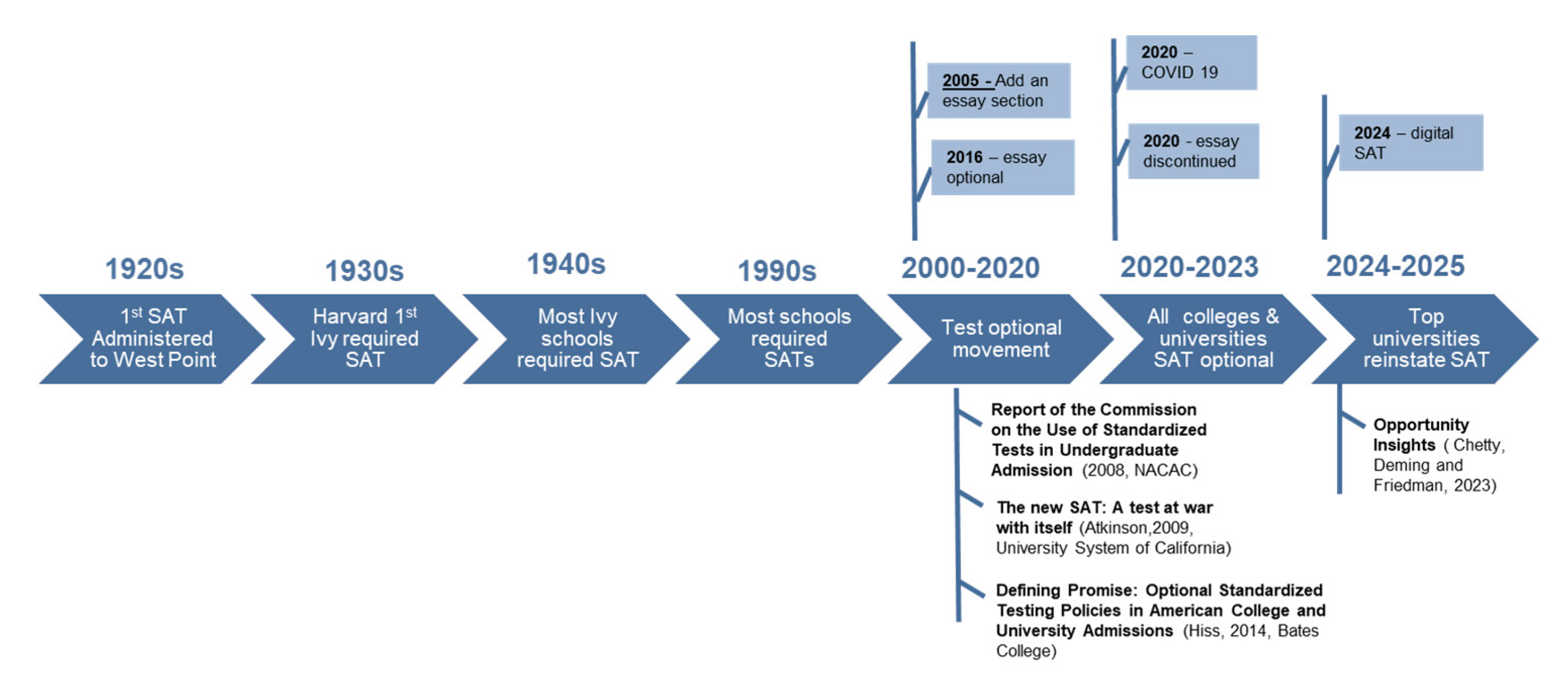
Figure 2.
The population distribution by race across all 50 states.
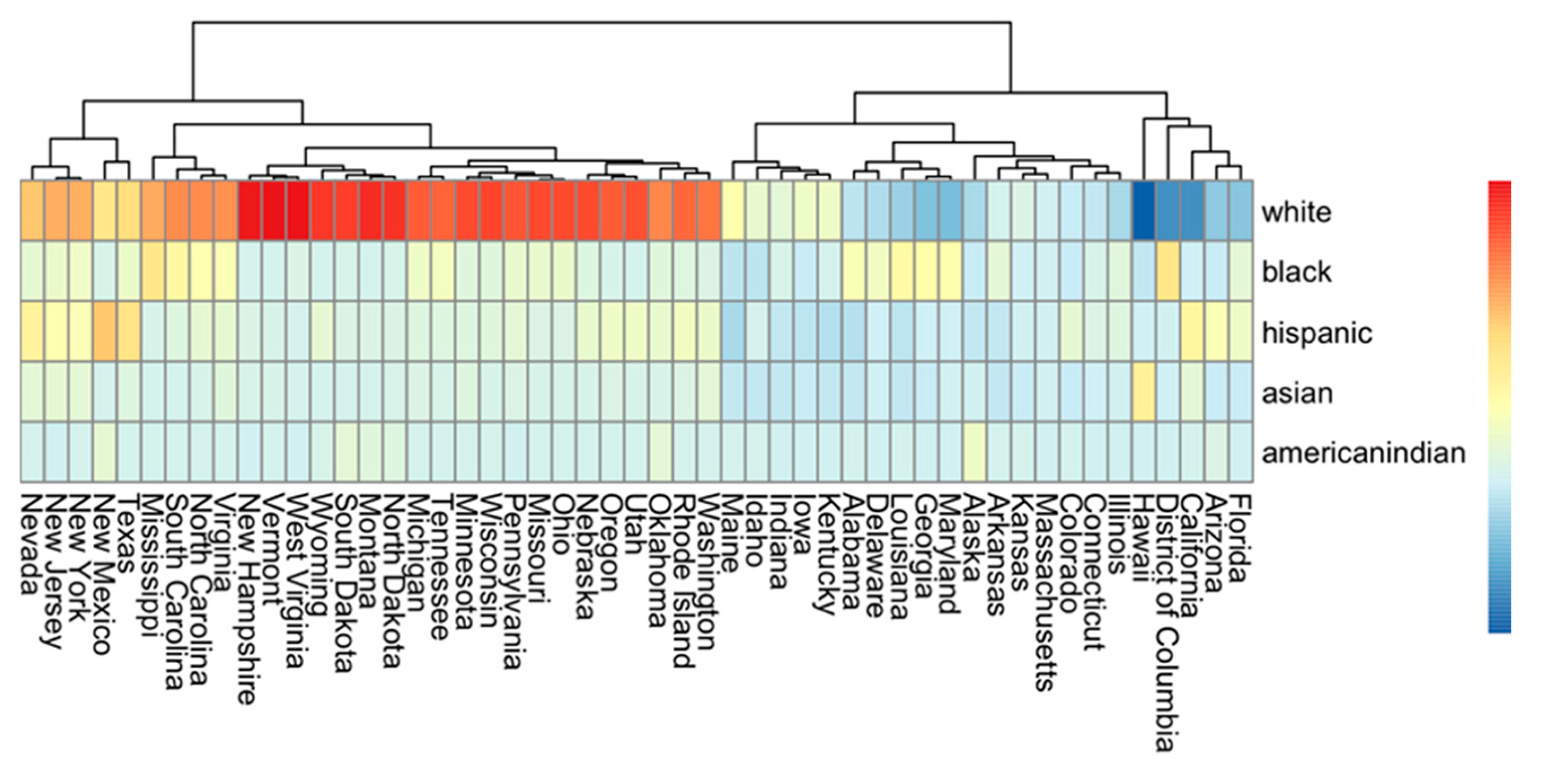
Figure 3.
Distribution of SAT scores and variables in the MA dataset.
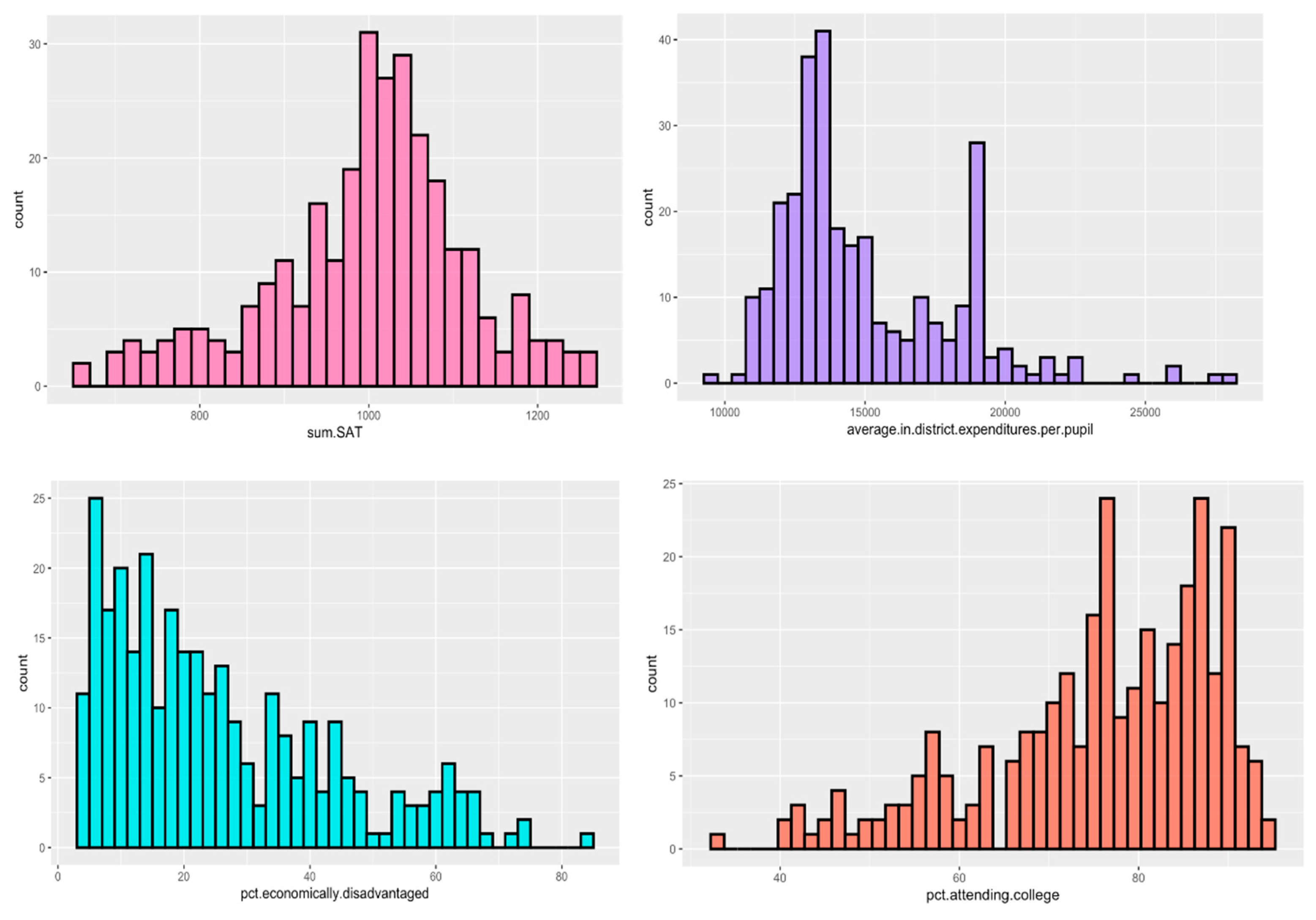
Figure 4.
Distribution of SAT scores and variables in the NYC dataset.
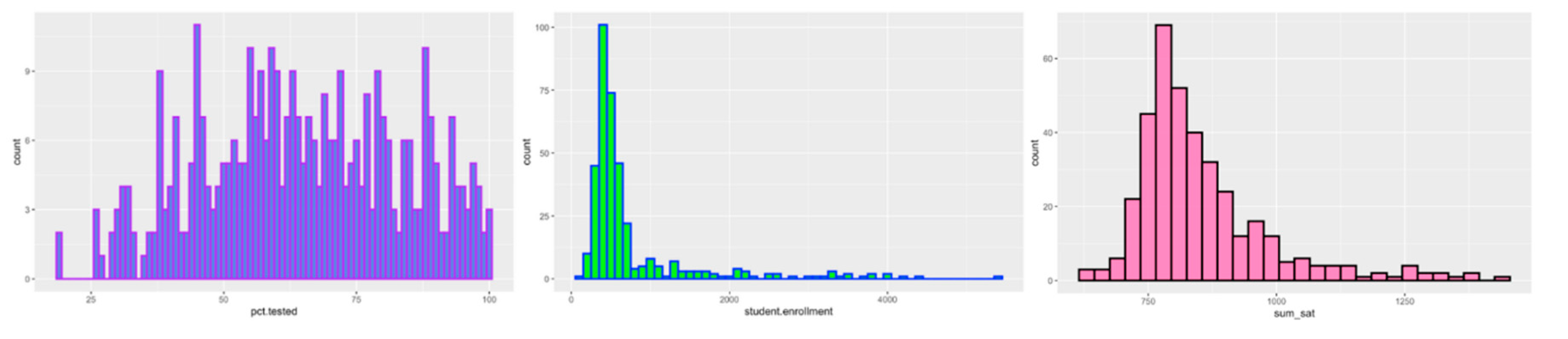
Figure 5.
Race distribution in Massachusetts dataset.
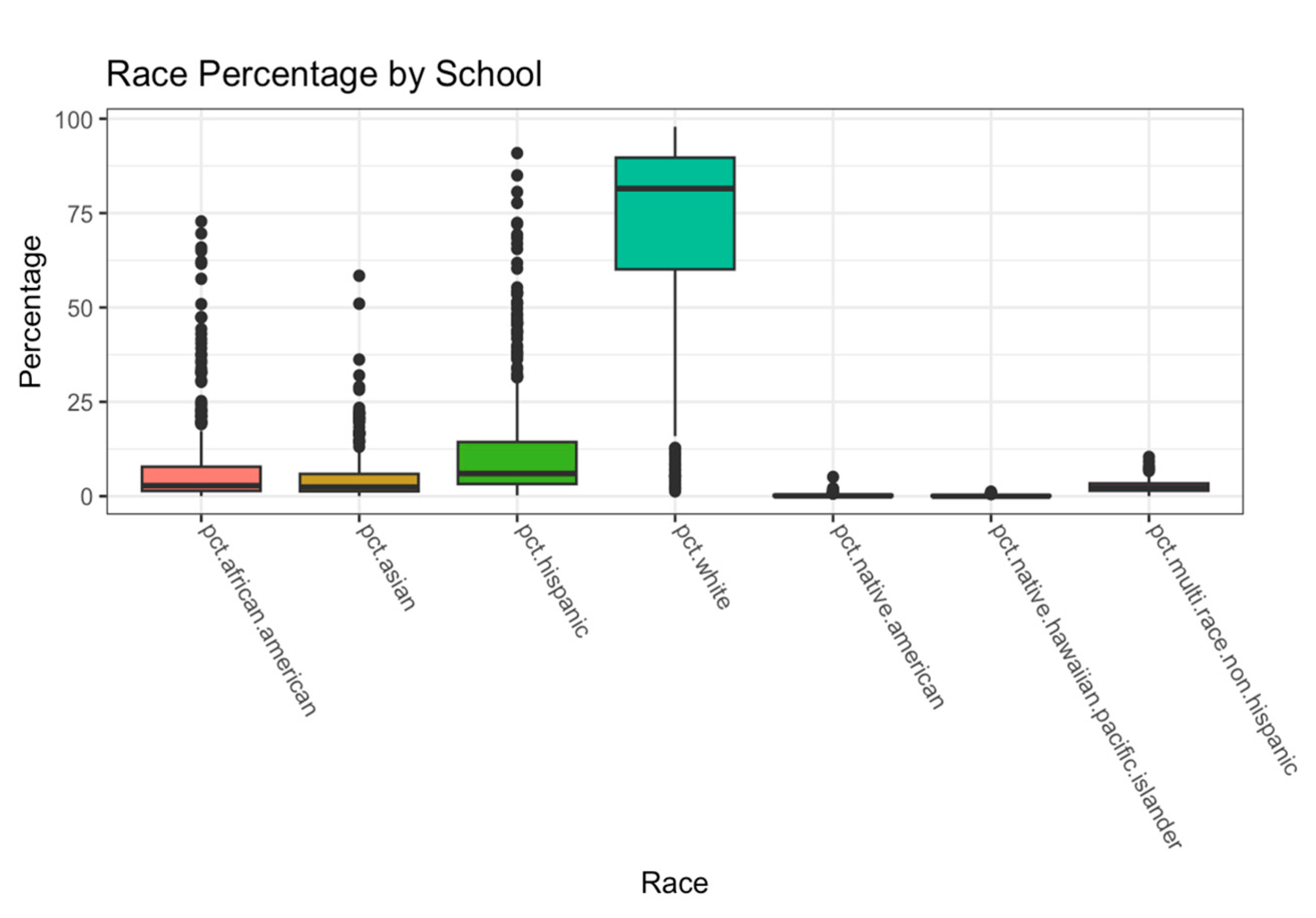
Figure 6.
Race distribution in NYC dataset.
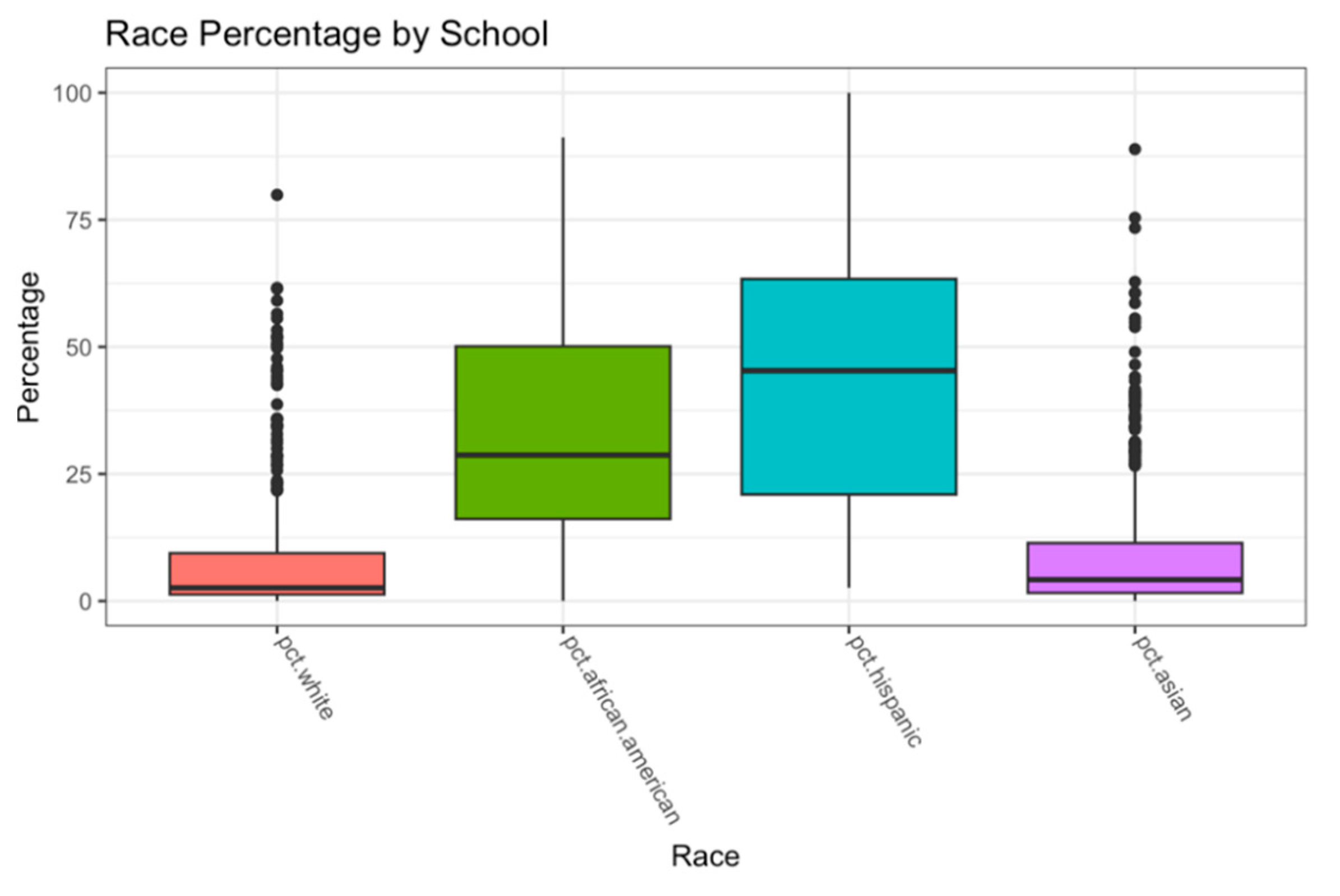
Figure 7.
Multicollinearity between variables in the Massachusetts dataset.
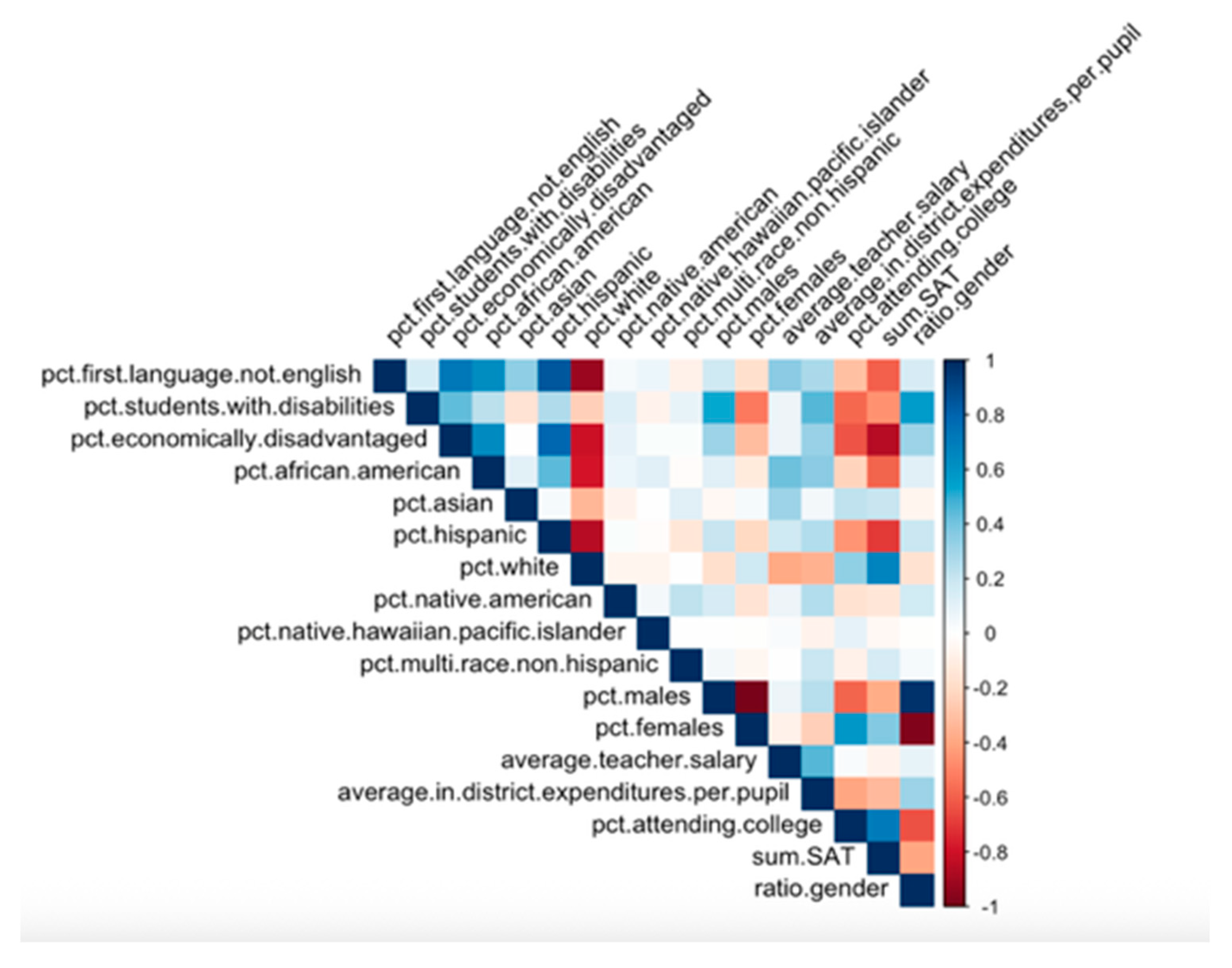
Figure 8.
Goodness of fit plots for MLR model in MA dataset.
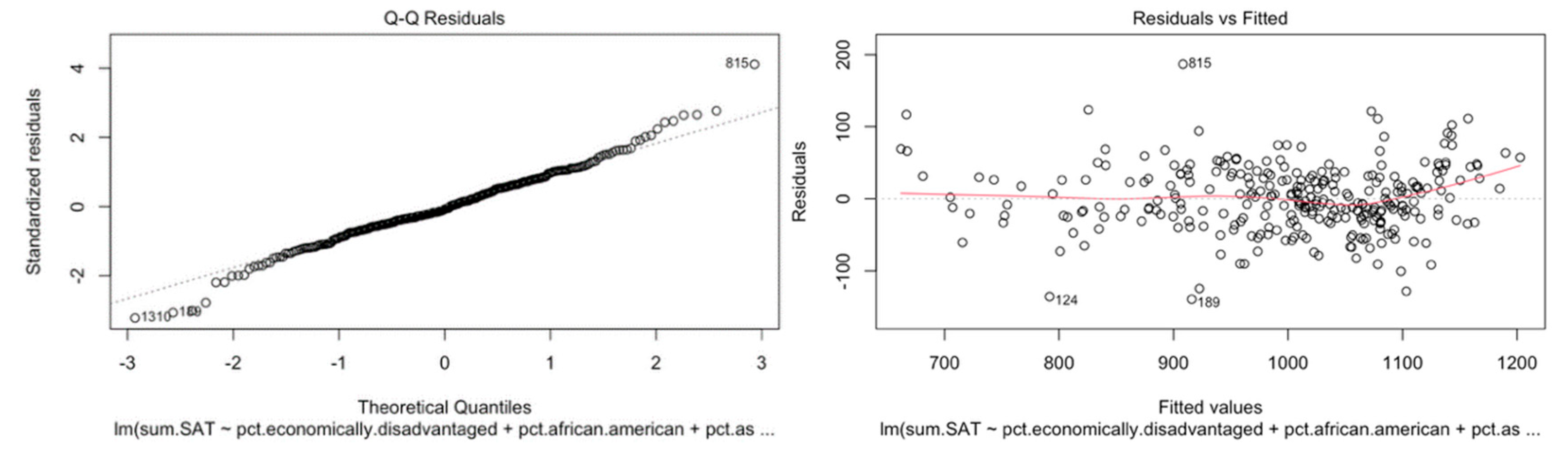
Figure 9.
Goodness of fit plots for MLR model in NYC dataset.
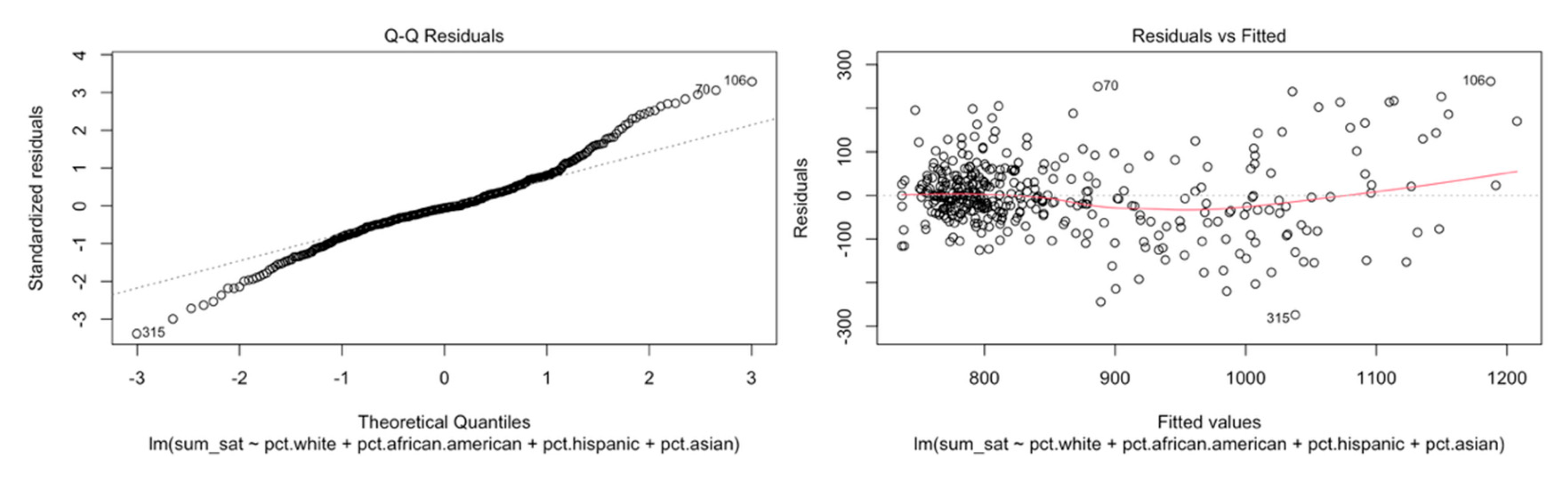
Figure 10.
Selection of the number of optimal variables (LASSO) in the MA dataset.
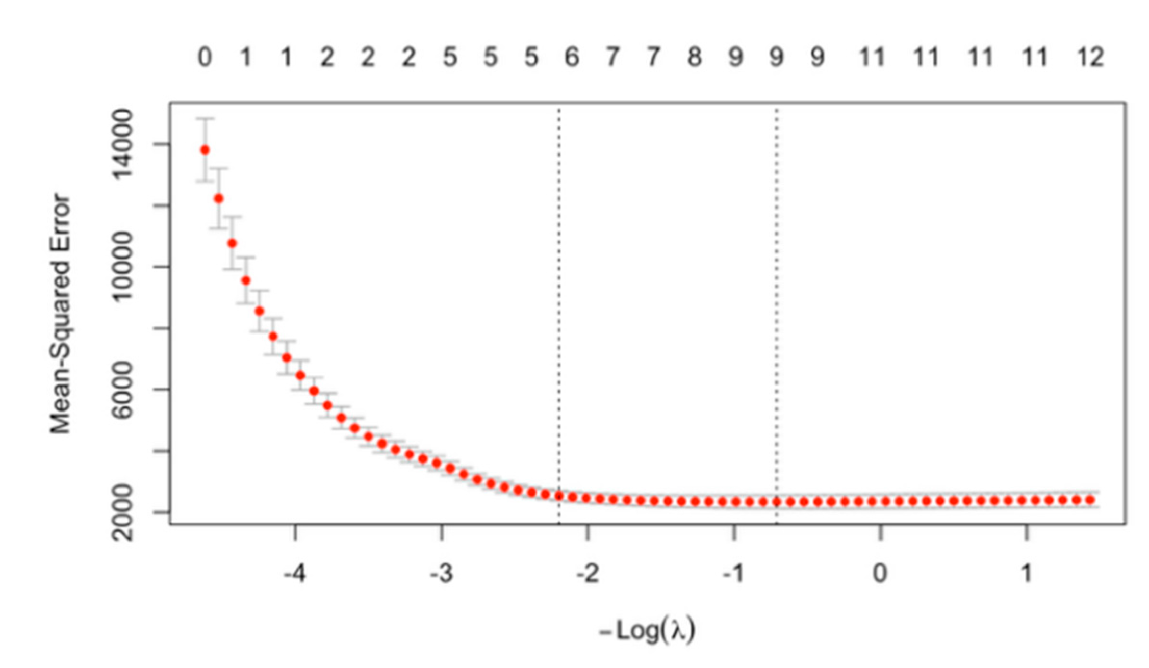
Figure 11.
Selection of the number of optimal variables (LASSO) in the NYC dataset.
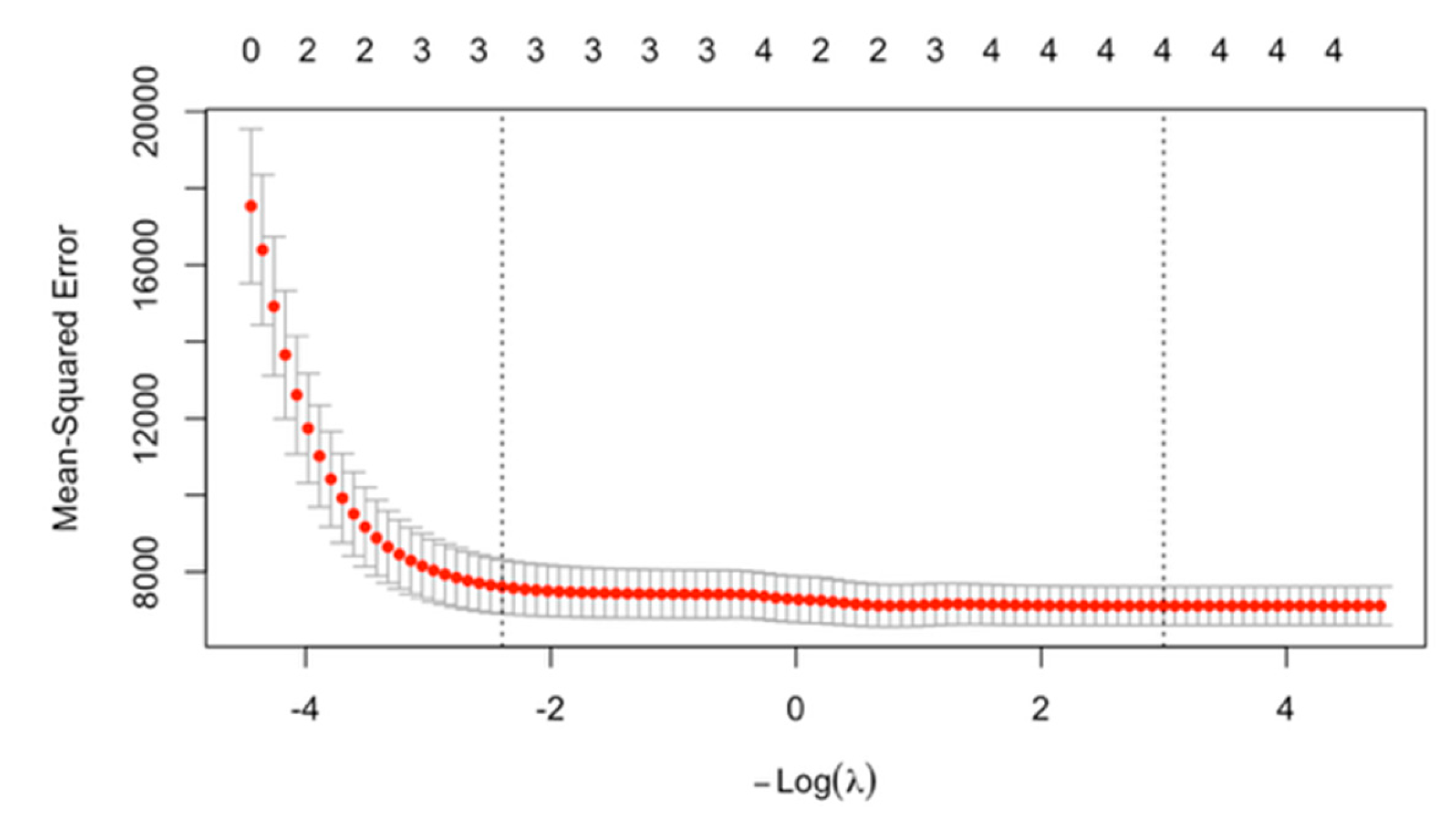
Figure 12.
The decision tree model of SAT scores and predictors in the MA dataset.
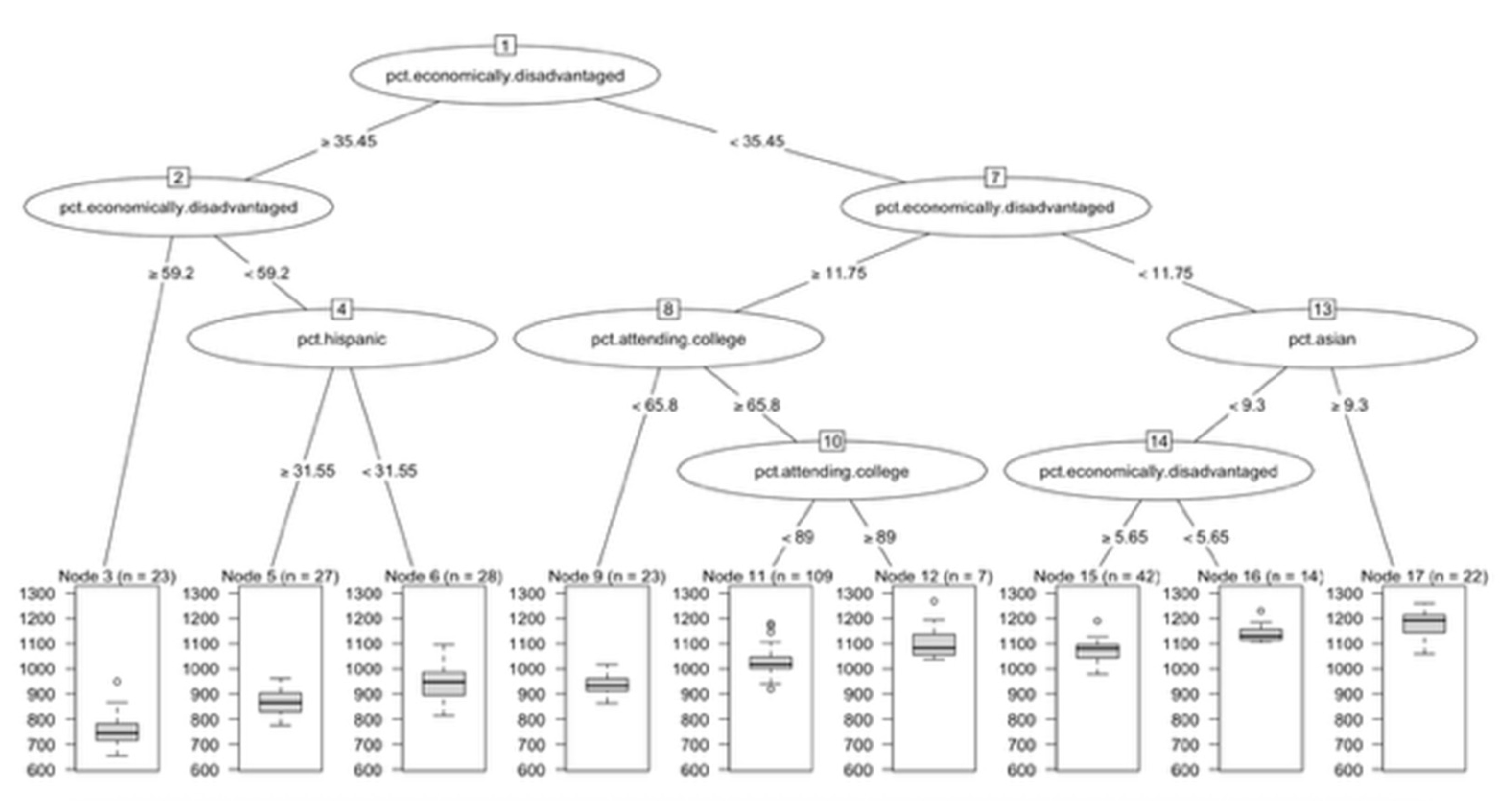
Figure 13.
The decision tree model of SAT scores and predictors in the NYC dataset.
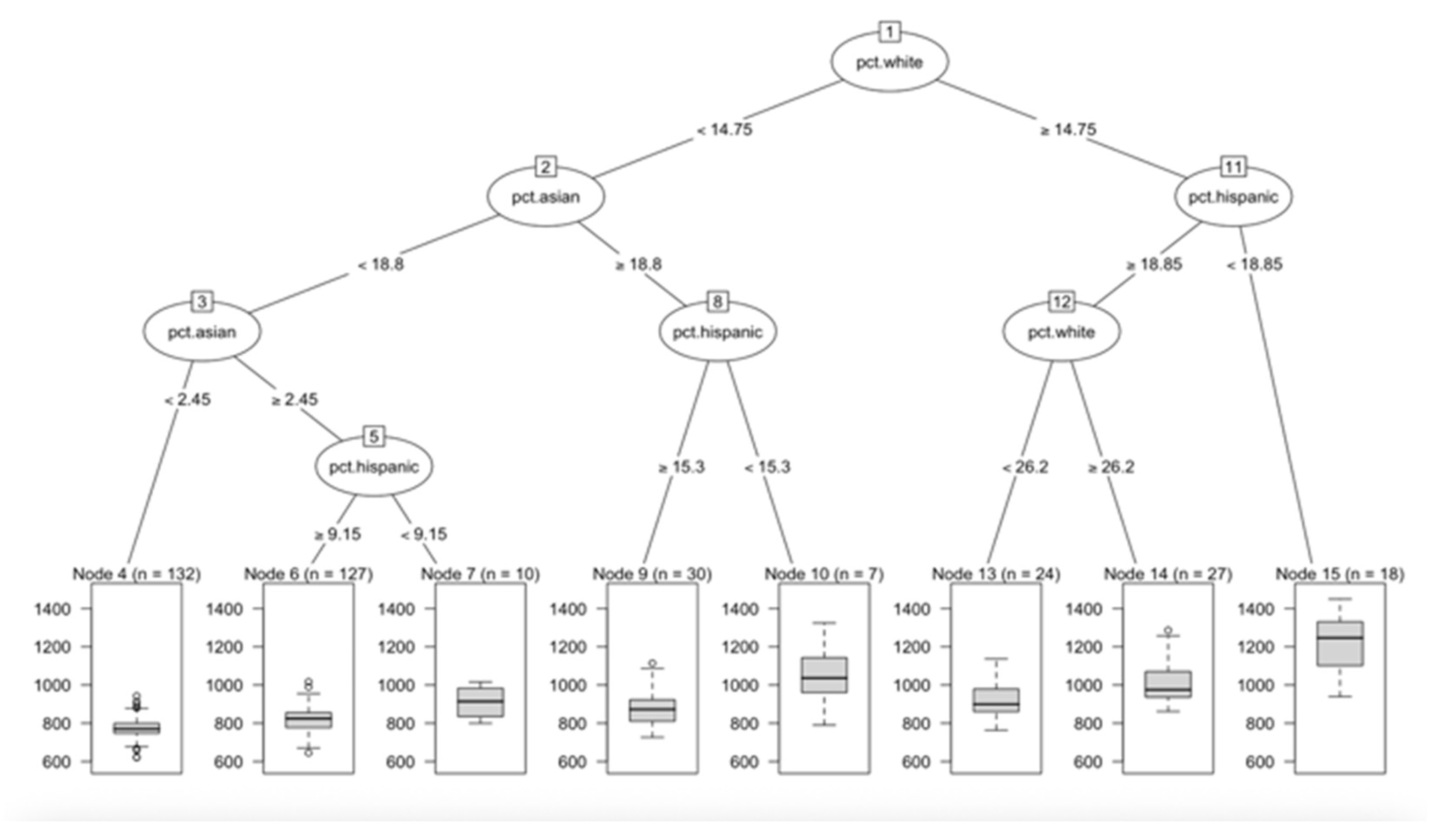
Figure 14.
SAT scores are tied to economically disadvantaged students and school expenditure using heat map analysis.
Figure 14.
SAT scores are tied to economically disadvantaged students and school expenditure using heat map analysis.
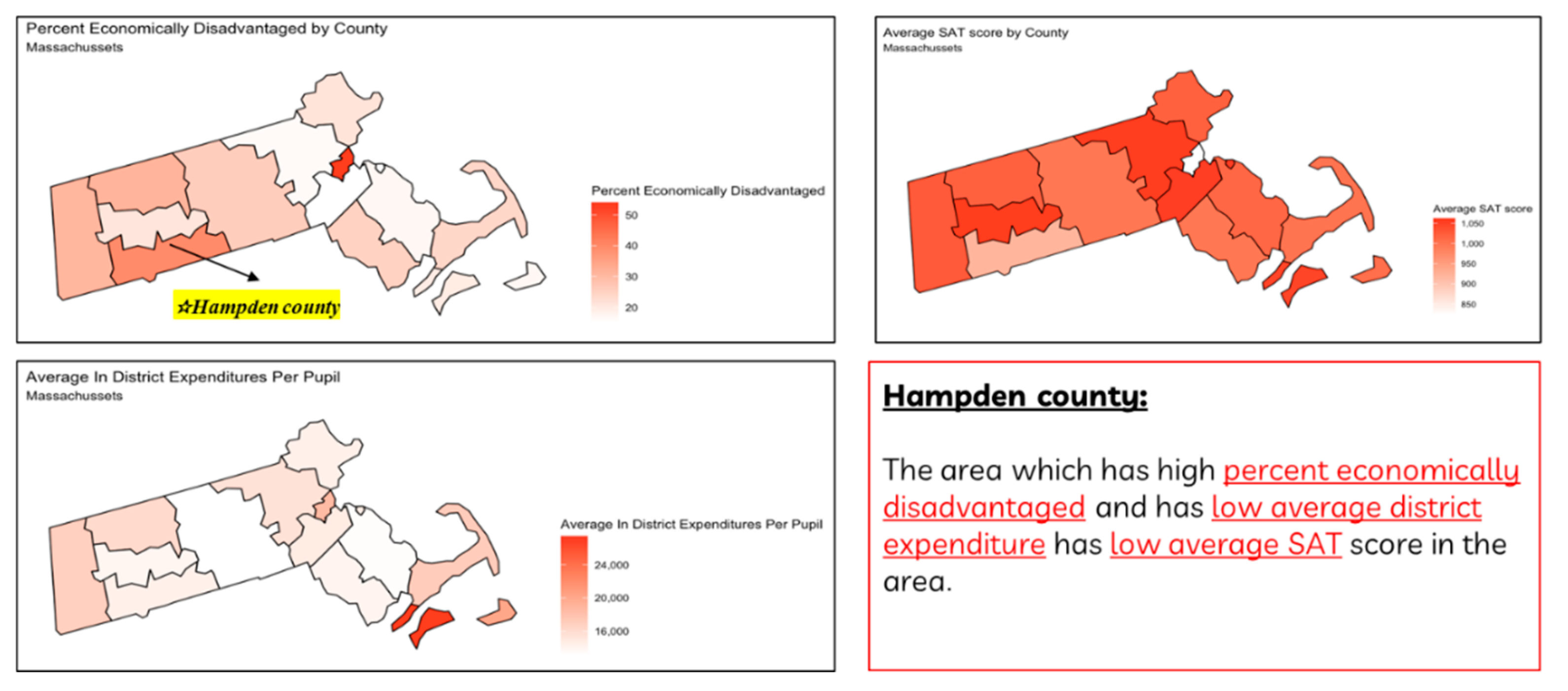

Table 1.
Variables correlated to SAT scores in Massachusetts Public Schools (A) and NYC Public Schools (B) using the Relaxed LASSO approach.
Table 1.
Variables correlated to SAT scores in Massachusetts Public Schools (A) and NYC Public Schools (B) using the Relaxed LASSO approach.
| Region | Relaxed LASSO Results | |
| Coefficient | Estimate | |
| Mass public schools | Pct. Native Pacific Islander | -11.928 |
| Pct. Native American | -11.567 | |
| Pct. Economically disadvantaged | -3.568 | |
| Pct. African American | -1.436 | |
| Pct. Hispanic | -0.281 | |
| Pct. Multi race non-Hispanic | 11.705 | |
| Pct. Attending college | 2.396 | |
| Pct. Asian | 2.185 | |
| NYC public schools | Pct. Hispanic | -12.08 |
| Pct. African American | -11.76 | |
| Pct. White | -7.71 | |
| Pct. Asian | -7.63 | |
Disclaimer/Publisher’s Note: The statements, opinions and data contained in all publications are solely those of the individual author(s) and contributor(s) and not of MDPI and/or the editor(s). MDPI and/or the editor(s) disclaim responsibility for any injury to people or property resulting from any ideas, methods, instructions or products referred to in the content. |
© 2026 by the authors. Licensee MDPI, Basel, Switzerland. This article is an open access article distributed under the terms and conditions of the Creative Commons Attribution (CC BY) license (http://creativecommons.org/licenses/by/4.0/).
Copyright: This open access article is published under a Creative Commons CC BY 4.0 license, which permit the free download, distribution, and reuse, provided that the author and preprint are cited in any reuse.


