
Submitted:
03 January 2026
Posted:
05 January 2026
You are already at the latest version
Abstract
This research paper focuses on determining the pressure wave propagation velocity in closed hydraulic pipes, a fundamental parameter relevant to a wide range of engineering applications, from aerospace to land-based and marine systems. It was indicated that, under transient conditions, the pressure wave propagation velocity depends, among other factors, on temperature, pressure, and the substitute bulk modulus. Furthermore, it was also indicated that accurate knowledge of this velocity is crucial for predicting pressure amplitudes during transient flows, including water-hammer phenomena. Finally, the analysis indicated that excessive pressure amplitudes in the pipe can lead to critical damage to the pipeline and increased vibration. Experimental investigations were carried out to determine the pressure wave propagation velocity in flexible steel-braided pipes and in a rigid pipe over a wide range of internal pressures.
Keywords:
machines
; hydraulic drive
; pipeline
; pressure pulsation
; wave phenomena
1. Introduction
Hydraulic systems remain an important part of contemporary engineering, even as electric and pneumatic actuators gain popularity. They are still widely used in industrial and land mobile equipment [1], as well as in marine [2] and aerospace applications [3], where their dependability, compact design, and high power-to-weight ratio are critical. In recent years, the range of uses for hydraulic technology has continued to grow. The hydraulic systems used in today’s transportation machinery consist of many different components, such as cylinders, hydraulic motors, pumps, valves, and throttling devices, assembled into complex dynamic structures in which every connection plays a key role in proper machine performance. As noted in [4,5], variations in components such as high-pressure hoses (flexible pipes), metal pipes, and fittings make it possible to connect hydraulic devices and adapt the layout of the hydraulic drive. An example of a hydraulic drive system in different transport machines is shown in Figure 1. Reference [6] further emphasizes that pipelines and fittings serve not only as connectors but also as elements that guide the fluid along the intended path within the system. With increasingly strict requirements for reducing energy use and implementing energy-efficient solutions in all types of transport machinery [7], research attention has shifted from analysing the energy demand of major hydraulic components to examining the consumption of auxiliary subsystems. Improvements to these subsystems, particularly pipelines, have created significant pressure on engineers and manufacturers to thoroughly assess all factors influencing the development of more efficient hydraulic drives.
The operating hydraulic system generates mechanical vibrations across a broad frequency range [8,9]. During operation, rapid fluctuations in the pressure of the working fluid naturally occur within the hydraulic circuit [10]. At the same time, transient states in hydrostatic systems are caused by forces resulting from sudden changes in the load on the power receiver or by rapid changes in the flow velocity of the working fluid caused by the control unit. In such situations, a rapidly changing fluid flow occurs in the supply pipeline, accompanied by waves of increased or decreased pressure. The sudden or wave-like increase (as well as decrease) in pressure accompanying unsteady fluid flow causes a heavy load on the pipe walls and system components, resulting in mechanical damage [11,12]. These loads can be impulsive or periodic. They can also cause self-excited vibrations of hydraulic pipes (see Figure 2) or cavitation [13,14,15], which leads to the formation of cavitation pits on the pipe walls, reduced system efficiency, noisy operation, or unstable operation of hydraulic receivers.
A special case of unsteady flow is water hammer, i.e., a strong pressure oscillation in a pressurised pipe caused by rapid, forced changes in the flow velocity of the liquid within a short period of time [16,17]. In physical terms, water hammer is caused by the inertia of the liquid moving in the pipeline, when its flow velocity undergoes a sudden change (increase or decrease). A sudden change in the velocity and volumetric flow rate of the liquid causes a local change in the ratio of kinetic to potential energy in the total energy of the liquid at a given flow cross-section, expressed as an increase or decrease in pressure in the liquid stream. Under conditions of very rapid deceleration of the flow velocity, there is a sudden decrease in kinetic energy, resulting in an increase in potential energy manifested by a large increase in pressure. The course of the water hammer phenomenon is significantly influenced by the compressibility of the liquid and the elasticity of the pipeline walls, i.e., their susceptibility to elastic deformation due to changes in hydrodynamic pressure. In extreme cases, this sudden increase in pressure can cause the critical tensile stresses in the pipeline walls to exceed allowable limits [18,19]. Scientific research on the description of unsteady fluid flow in closed (pressurised) pipes was initiated by Joukowsky as early as 1898 [20]. In the cited paper, a simplified relationship between the pressure increase (Δp) and the change in the average flow velocity (Δv) was presented for the first time:
where: ρ0 – liquid density; c0 – pressure wave propagation velocity.
From the point of view of accurately reproducing actual transient waveforms through numerical simulations, it is important to correctly determine the pressure wave propagation velocity (c0). This allows correct (i.e., close to actual) numerical simulation results to be obtained with respect to the amplitudes and frequencies of pressure changes in the pipe. The pressure wave propagation velocity in the pipeline determines the pressure wavelength. The pressure wavelength is a key parameter that is taken into account when designing effective branch or bypass pressure pulsation dampers [21]. The pressure wave propagation velocity can be determined from the formula [22,23,24]:
where: Ec – bulk modulus of the working fluid; D – internal diameter of the pipe; E – Young’s modulus of the pipe material; gp – wall thickness of the pipe; c1 – constant.
The constant c1 depends on the method of fixing the pipeline and can be determined using one of the following relationships, as given in [24].
For a pipe fixed at one end:
For a pipe fixed at both ends (with no axial displacement):
For a pipe with longitudinal compensation:
where vp – Poisson’s ratio of the pipe material.
Equation (2) is valid assuming that, during the transient state, there is only unidirectional stress in the pipe walls, therefore, its application is limited to thin-walled pipes. A hydraulic pipe is considered thin-walled if it satisfies the assumptions of a momentless membrane shell. The stress and deformation state of a membrane shell can be described by the Laplace equations, and its relative thickness mw must satisfy the following condition [25,26]:
In modern hydrostatic drive systems, due to the pressure ranges used, the relative thickness mw often significantly exceeds the limit value of 0.025. In the case of thick-walled pipes, it is necessary to use a three-dimensional description of the stress state, which significantly complicates the derivation of the relationship for c0 [25,26]. Equation (2) is also not applicable to flexible pipes, as manufacturers typically do not provide data on the Young’s modulus E of the pipe material. This is particularly true when several steel braids are used in the construction of a flexible pipe. For this reason, it should be assumed that the use of Equation (2) to determine the pressure wave propagation velocity is limited in practice and can often lead to erroneous results. The article proposes determining the pressure wave propagation velocity on the basis of an experimentally determined substitute bulk modulus Ez, which accounts for the deformation of the working fluid and the hydraulic pipe, according to the formula for c0d, i.e., the propagation velocity of a sound wave in a fluid [24]:
By replacing the liquid bulk modulus Ec with the substitute modulus Ez (describing the deformation of the liquid and the pipe walls), a relationship describing the propagation velocity of the pressure wave in the hydraulic pipe is obtained in the form:
Such an approach makes it possible to account for the actual mechanical behavior of the pipe–fluid system without relying on simplified geometric assumptions or incomplete material data. Consequently, the experimentally derived modulus Ez ensures a more reliable estimation of the pressure wave propagation velocity, particularly in systems employing flexible or thick-walled hydraulic pipelines.
2. Method for Determining the Substitute Bulk Modulus of the Working Fluid and Hydraulic Pipe
An approximate analysis of a hydraulic system assumes, among other things, that hydraulic oil is incompressible. This assumption leads to an approximate solution. In reality, oil subjected to external pressure undergoes a decrease in volume. This susceptibility of oil to deformation under changing pressure is largely related to the presence of air in the oil. A measure of compressibility is the compressibility coefficient βc, defined as [27]:
The reciprocal of the compressibility coefficient is the bulk modulus Ec, determined from the relationship [27]:
where: V – liquid volume; p – pressure.
The bulk modulus Ec therefore expresses the relative decrease in liquid volume caused by an increase in pressure. It should also be mentioned that the compression of liquids is accompanied by the release of heat. If the process is slow, the heat is dissipated and the temperature of the liquid remains constant. However, during rapid compression, heat is transferred to the liquid, raising its temperature. In the first case, an isothermal transformation occurs, and the corresponding isothermal bulk modulus is EcT, whereas in the second case an isentropic transformation occurs, and the isentropic bulk modulus is Ecs. The relationship between the two moduli is expressed by the following equation [27]:
where χ – is the adiabatic exponent (for commonly used oils, χ = 1.16 – 1.18) [27].
The value of the isothermal bulk modulus EcT depends on temperature and pressure [28,29,30]. The numerical values of the isothermal bulk modulus EcT for commonly used hydraulic oils are known and are generally reported in the literature [31,32]: EcT = (1.25 – 2.0) × 103 MPa. Lower values are usually assumed for oils with lower specific gravity. For water and water emulsions, EcT = 2 × 10³ MPa can be assumed. The numerical value of the isothermal bulk modulus EcT increases with increasing pressure (by approx. 1% per 2 MPa increase in pressure in the range up to 20 MPa), while it decreases with increasing temperature (by approx. 1% per 2 °C increase in temperature in the range up to 100 °C) [32,33]. These data refer to non-aerated oil. In practice, however, during the operation of a hydraulic system, the working fluid is not a homogeneous liquid. It is a mixture of oil and air bubbles with a diameter of 0.05–0.5 mm [33]. Due to the limited size of the tanks, a significant portion of the bubbles in the oil is drawn back into the pump and further broken up, resulting in an equilibrium state in the operating system, expressed as a specific percentage of air undissolved in the oil. Due to the significant influence of undissolved air in oil on liquid compressibility, it is necessary to measure the air content during hydraulic system operation in order to determine the bulk modulus of the mixture. However, such measurements require specialised equipment and are costly [32,33]. The main problem in measuring the amount of undissolved air in oil is achieving sufficiently high measurement accuracy. This is evidenced by the fact that the presence of only 1% undissolved air in oil causes a multiple increase in the compressibility of the mixture relative to the compressibility of oil [31,33]. The effect of liquid compressibility on the system can be increased by elastic deformation of the pipe walls, especially when flexible pipes are used [27,34].
In order to experimentally and reliably determine the substitute bulk modulus EzT, taking into account the compliance of the fluid (containing air under real conditions) and hydraulic pipes, an experimental method is used (see Figure 3). A thick-walled cylinder (non-deformable) filled with liquid and connected to a hydraulic pipe with an initial volume V₀ is sealed with a piston and piston rod loaded with a force F. Based on Equation (10), replacing the derivatives with increments of individual parameters, it can be written:
The change in substitute volume ΔVz under the influence of a pressure increase is determined by superposition of the liquid deformation in the pipe, ΔVol, and the pipe deformation, ΔVp, reduced by the change in volume ΔVu of the measuring system itself (without the hydraulic pipe):
Based on the measurements taken, the characteristics of the volumetric deformations of the hydraulic pipe (filled with liquid) are obtained in the form of a nonlinear relationship between the relative volume change ΔVz/V0 and the pressure p (see Figure 4). In order to obtain a constant value of the substitute bulk modulus of the hydraulic pipe in a specific pressure range or at a specific pressure value, the relative deformation characteristics are linearised using a secant or a tangent.
A measure of the isothermal substitute bulk modulus (at constant temperature) is the following relationship:
where: i = 1 corresponds to the tangent modulus; i = 2 corresponds to the secant modulus.
In standard calculations, tangent values are used. When volume changes need to be taken into account, secant values are used [27].
3. Method for Testing the Substitute Bulk Modulus
The diagram of the measuring station is shown in Figure 5. The station is equipped with pipes for testing with the following geometric dimensions: l = 1 m (pipe length) and D = 9 mm (internal diameter), with an internal volume V0. Three different pipes can be mounted on the station. A manually operated pump supplies the required amount of working fluid to the system, thereby producing the required discharge pressure p, which is read on the pressure gauge.
The system of cut-off valves adopted at the measuring station ensures the following functions during measurements, using pipe 12 in Figure 5 as an example:
Step 1: filling the working chamber of the hand-operated pump (cut-off valves 3, 5, 6, 7, and 8 closed);
Step 2: supplying the working fluid to the system to ensure that the required discharge pressure p is obtained in the system and in the pipe under test (cut-off valves 3, 7, and 8 closed; cut-off valves 5 and 6 open);
Step 3: zeroing the discharge pressure p in the system (cut-off valves 5, 6, 7, and 8 closed; cut-off valve 3 open);
Step 4: measuring the volume increase ΔVz in the tested pipe 12 under the influence of the set discharge pressure p (cut-off valves 5, 7, and 8 closed; cut-off valves 3 and 6 open).
The combined increase in volume of the pipe and the working fluid, ΔVz, is measured by reading the liquid level in the measuring cylinder after opening the shut-off valve. The increase in volume ΔVz is determined as the difference between these liquid levels in the measuring cylinder, minus the correction for the instrument itself ΔVu (determined without the pipe). The scale marked on the wall of the measuring cylinder allows the increase in the volume of the pipe together with the working fluid to be read. Valves 9, 10, and 11 are used to vent the tested pipes.
Figure 6 shows the measuring station (test rig) used to carry out the measurements according to the diagram in Figure 5.
An example of the characteristics of volumetric deformations of a hydraulic pipe, , for a flexible single-braid pipeline tested on the test rig is shown in Figure 7.
, for a flexible single-braid pipe (l = 1 m; D = 9 mm; oil: HL 46; temperature T = 323 ± 2 K).
Based on these characteristics, the values of the isothermal substitute bulk modulus of individual hydraulic pipes were determined, as shown in Figure 8.
In these tests, the EzT value is given by ctg(α₂), i.e., the slope of the tangent at individual pressure values at a constant oil temperature. For example, Figure 7 shows the tangent over the range 0–13 MPa, i.e., the pressure range for the flexible pipe. According to Equation (14), for this range, the numerical value of the EzT modulus is 518 MPa and, according to Equation (7), c0 = 769 m/s (ρ0 = 875 kg/m3 was assumed).
4. Experimental Studies of Pressure Wave Propagation Velocity
The authors of [30] measured the speed of sound, which corresponds to the pressure wave propagation velocity in biodiesel fuel supply pipes. Using an ultrasonic method, they determined the pressure wave propagation velocity in a metal pipe to be c0 = 1300–1380 m/s, but only in the low-pressure range of 0.02–0.6 MPa. As part of this research work, tests were carried out to determine the pressure wave propagation velocity c₀ depending on the pipe material and at higher working pressures commonly used in hydrostatic systems. The diagram of the test stand is shown in Figure 9. Figure 10 shows the measuring stand (test rig) corresponding to the diagram for testing pressure wave propagation velocity.
The tests consisted of recording the pressure curve at the pump (p1), at the end of the rigid pipe (p2), and at the end of the flexible pipe (p3) after a step change of directional control valve 12 to initiate flow through throttle valve 13 (step change in load). Pressures p1, p2, and p3 were measured by pressure sensors 9, 10, and 11, respectively, as shown in Figure 9. By determining the time delay Δtel between the onset of the pressure increase at p₃ (end of the flexible pipe) and the onset of the pressure increase at p₂ (beginning of the flexible pipe), the pressure wave propagation velocity c0el was calculated for the flexible pipe (one or two steel braids, D = 9 mm). In a similar way, the pressure wave propagation velocity for the steel pipe (D = 9 mm, wall thickness gp = 1.5 mm), c0szt, was determined: the time delay Δtszt between the onset of the pressure rise at the end of the rigid pipe (p₂) and the onset of the pressure rise at the beginning of the rigid pipe (p₁) was measured. The following relationship was used:
where: ls = 9 m – length of the rigid pipe; Δtszt – time delay for the rigid pipe; le = 8 m – length of the flexible pipe; Δtel – time delay for the flexible pipe.
The following conditions were ensured during the tests: the working fluid was HL 46 hydraulic oil; the working fluid temperature was T = 323 ± 2 K; the main pump discharge pressure was p1 = 0–22 MPa; the main pump suction pressure was ps = 0.01 MPa; and the main pump shaft rotational speed was ns = 25 s⁻¹ (1500 rpm).
The following measuring equipment was used to record instantaneous pressure waves at the appropriate points on the hydraulic pipes: strain-gauge pressure sensors with a power supply unit and a 0–10 V signal output; electrically shielded signal cables to reduce external interference; a Tektronix TDS-224 digital oscilloscope with a TDS2CM expansion module; a computer; and Tektronix WaveStar software.
In order to determine the accuracy of pressure waveform recording (by determining the maximum systematic uncertainty), the individual uncertainties occurring throughout the entire measurement chain, from the sensor to the amplifier and computer, must be summed. The pressure wave propagation velocity was determined on the basis of several repeated measurements of the signal recording delay between successive strain gauge pressure sensors. The measurement uncertainty of the pressure wave propagation velocity was estimated at δpmax = 2.5%. Examples of pressure waveforms in the test system for a rigid pipe and a flexible pipe (one steel braid) connected in series are shown in Figure 11 and Figure 12 for different flow rates and pressures in the pipe. Figure 13 illustrates the relationship between pressure wave propagation velocity and pressure for different hydraulic pipes.
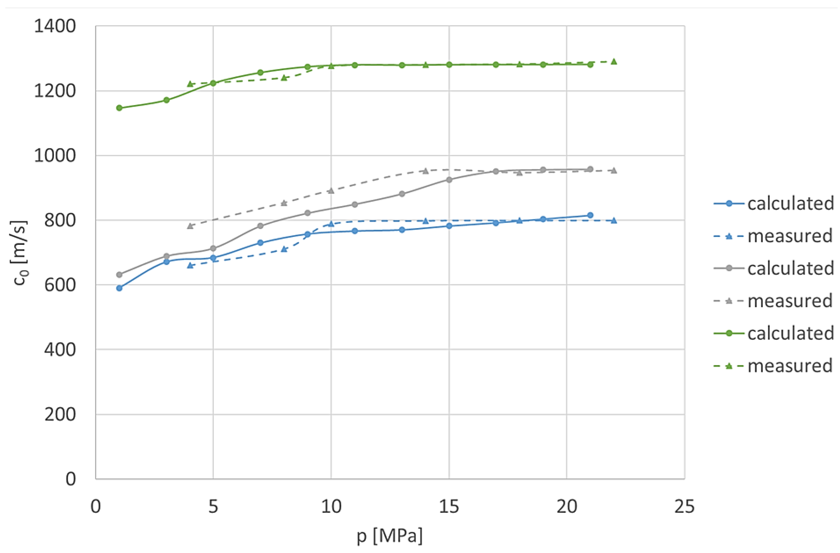
Based on the calculated substitute bulk modulus, the velocity c0 was calculated for the three analysed pipes and then compared with the experimentally obtained results, as described below (Figure 14).
The obtained results show good agreement between the proposed method for calculating the pressure wave propagation velocity, based on determining the substitute bulk modulus, and the experimentally obtained results. For all tested pipes, the pressure wave propagation velocity increases nonlinearly as the average internal pressure increases. Changes in velocity are more pronounced at lower pressure ranges, while the rate of change decreases at higher average pressures. The highest propagation velocities were recorded in rigid steel pipes, while flexible pipes with one steel braid exhibited the lowest velocities due to their higher compliance. The values calculated using the experimentally determined substitute bulk modulus showed high correlation with the direct experimental measurements, with a maximum difference of 7–8%, which is within the estimated measurement uncertainty.
5. Conclusions
The paper proposes a method for determining the pressure wave propagation velocity in hydraulic pipes based on an experimentally determined substitute bulk modulus that takes into account the deformability of the fluid and the pipe itself. The proposed method is a hybrid one, combining experimental measurements of the substitute bulk modulus and numerical calculations of the pressure wave propagation velocity in the pipe This method is particularly applicable to flexible pipes and rigid thick-walled pipes. Comparing the results obtained on the basis of the empirically determined substitute bulk modulus with those from direct measurements, it can be concluded that they differ by no more than 7–8% and thus fall within the measurement uncertainty, taking into account both the recording of instantaneous pressure waves and the method of determining the substitute bulk modulus. Based on the measurements carried out, empirical equations were obtained that describe the relationship between the pressure wave propagation velocity (c₀) and the static pressure measured at the midpoint of the tested pipes. These equations were obtained in the pressure range of 4–22 MPa in the following form:
Rigid steel pipe with relative thickness mw = 0.167 (D = 9 mm; gp = 1.5 mm):
c0s = -0.2906p2 + 11.329p + 1179.5;
Flexible pipe with two steel braids:
c0e2 = -0.7895p2 + 30.074p + 672.02;
Flexible pipe with one steel braid:
c0e1 = -0.8142p2 + 28.772p + 556.4.
For all tested pipes, it can be concluded that as the average pressure in the pipe increases, the pressure wave propagation velocity increases, and this relationship is nonlinear. At higher average pressures in the pipe, changes in velocity are smaller than those at lower pressures.
Author Contributions
Conceptualization, M.S. and M.K.; methodology, M.S., L.J.; software, M.S., P.S., M.K.; validation, M.S., L.J.; formal analysis, M.S., L.J. and M.K.; investigation, M.S., M.K.; resources, M.S., L.J. and P.S.; data curation, M.S., P.S., M.K.; writing–original draft preparation, M.S., M.K.; writing–review and editing, M.S., L.J. and M.K.; visualization, M.K. and P.S.; supervision, M.S. and M.K.; project administration, M.S. and M.K.; funding acquisition, M.S., P.S., L.J. and M.K. All authors have read and agreed to the published version of the manuscript.
Funding
This research received no external funding.
Data Availability Statement
All data included in this research are available upon request from the corresponding author.
Conflicts of Interest
The authors declare no conflict of interest.
References
- Kumari, N.; Ganesh, U.; Bharat, P.; Swapnil, C.; Vijaya, R. A tractor hydraulic assisted embedded microprocessor-based penetrometer for soil compaction measurement. J. Terramechanics 2023, 110, 1–12. [Google Scholar] [CrossRef]
- Wang, Y.; Zhai, B.; Chen, Y.; Huo, L.; Du, L.; Liu, T.; Zhang, A.; Zhang, Q. Design and performance research of water–glycol deep-sea valve-controlled hydraulic cylinder system based on on-line regulation of ambient pressure. Ocean Engineering 2024, 313, 1–16. [Google Scholar] [CrossRef]
- Liu, X.; Li, D.; Qi, P.; Qiao, W.; Shang, Y.; Jiao, Z. A local resistance coefficient model of aircraft hydraulics bent pipe using laser powder bed fusion additive manufacturing. Experimental Thermal and Fluid Science 2023, 147, 1–11. [Google Scholar] [CrossRef]
- Wei, Q.; Huailiang, Z.; Wenqian, S.; Wei, L. Stress response of the hydraulic composite pipe subjected to random vibration. Composite Structures 2021, 255, 1–8. [Google Scholar] [CrossRef]
- Karpenko, M.; Stosiak, M.; Šukevičius, Š.; Skačkauskas, P.; Urbanowicz, K.; Deptuła, A. Hydrodynamic Processes in Angular Fitting Connections of a Transport Machine’s Hydraulic Drive. Machines 2023, 11, 355. [Google Scholar] [CrossRef]
- Nishimura, S.; Matsunaga, T. Analysis of response lag in hydraulic power steering system. JSAE Review 2000, 21, 41–46. [Google Scholar] [CrossRef]
- European Commission. Communication from the commission to the European parliament, the council, the European economic and social committee and the committee of the regions. Brussels. 2011. Available online: https://eur-lex.europa.eu/LexUriServ/LexUriServ.do?uri=COM:2011:0885:FIN:EN:PDF.
- Ren, Y.; Tang, H.; Xiang, J. Experimental and numerical investigations of hydraulic resonance characteristics of a high-frequency excitation system. Mechanical Systems and Signal Processing 2019, 131, 617–632. [Google Scholar] [CrossRef]
- Stosiak, M.; Karpenko, M.; Ivannikova, V.; Maskeliūnaitė, L. The impact of mechanical vibrations on pressure pulsation, considering the nonlinearity of the hydraulic valve. Journal of Low Frequency Noise, Vibration and Active Control 2025, 44, 706–719. [Google Scholar] [CrossRef]
- Stosiak, M.; Bury, P.; Karpenko, M. The influence of hydraulic hose length on dynamic pressure waveforms including wave phenomena. Sci. Rep. 2025, 15, 31548. [Google Scholar] [CrossRef]
- Li, Y.; Liu, W.; Ren, J.; Cui, M.; Nikolaitchik, M. A new framework incorporating long short-term memory and physics-informed neural networks for solving transient fluid flow problems in turbine vanes. International Communications in Heat and Mass Transfer 2025, 168, 109482. [Google Scholar] [CrossRef]
- Lorenz, J.; Hildner, M.; Bogert, W.; Zhu, B.; Yee, S.; Fazeli, N.; Shih, A. Modeling of the high-viscosity fluid transient flow for material deposition in direct ink writing. Additive Manufacturing 2025, 109, 104836. [Google Scholar] [CrossRef]
- Tong, Z.; Shu, Z.; Liu, D.; Tong, S. Investigating flow-induced vibration in pump-turbines using a multi-scale fluid-structure interaction approach considering clearance flow effects. Sustainable Energy Technologies and Assessments 2025, 82, 104487. [Google Scholar] [CrossRef]
- Xi, X.; Liu, C.; Pan, Y.; Zhang, R.; Song, S.; Xu, S.; Liu, H. Numerical investigation of in-nozzle cavitation and flow characteristics in diesel engines using a multi-fluid quasi-VOF model coupled with a cavitation model. International Journal of Heat and Fluid Flow 2025, 115, 109858. [Google Scholar] [CrossRef]
- Guo, M.; Liu, C.; Liu, S.; Zhang, J.; Ke, Z.; Yan, Q.; Khoo, B. On the transient cavitation characteristics of viscous fluids around a hydrofoil. Ocean Engineering 2023, 267, 113205. [Google Scholar] [CrossRef]
- Deng, S.; Yi, L.; Li, X.; Yang, Z.; Zhang, N. A diagnostic model for hydraulic fracture in naturally fractured reservoir utilising water-hammer signal. Engineering Fracture Mechanics 2025, 325, 111347. [Google Scholar] [CrossRef]
- Dong, X.; Zhu, H.; Wang, X.; He, L.; Liu, Z.; Gong, W.; Zhan, L.; Tang, J.; Yi, X. Research and application of hydraulic fracturing fluid entry depth detection method based on water-hammer signal. Geoenergy Science and Engineering 2025, 246, 213556. [Google Scholar] [CrossRef]
- Cao, Y.; Ma, H.; Guo, X.; Chen, W.; Wang, W.; Zhao, T.; Lin, J. Fluid pulsation excitation characterization and pipeline vibration response analysis. Mechanical Systems and Signal Processing 2025, 231, 112691. [Google Scholar] [CrossRef]
- Wang, Y.; Xue, D.; Wu, B.; Wang, X.; He, L. Failure analysis and forming process optimization of high-pressure sealed hydrogen pipelines under stress assembly conditions. Engineering Failure Analysis 2025, 182, 110084. [Google Scholar] [CrossRef]
- Joukowsky, N. Uber den hydraulischen Stoss in Wasserleitungsróhren (On the hydraulic hammer in water supply pipes). Mómoires de IF Acadćmie Impćriale des Sciences de St.-Pćtersbourg in German. 1900, 5. [Google Scholar]
- Kudźma, Z. Tłumienie pulsacji ciśnienia i hałasu w układach hydraulicznych w stanach przejściowych i ustalonych; Oficyna Wydawnicza Politechniki Wrocławskiej, 2012; 261 p, in Polish; ISBN 978-83-7493-681-1. [Google Scholar]
- Herer, C.; Gutowska, I. Thermal-Hydraulic Principles and Safety Analysis Guidelines of PWRs and iPWR-SMRs; Academic Press (Elsevier Science & Technology), 2025; 250 p, ISBN 9780323904940. [Google Scholar]
- Thorley, A. Fluid Transients in Pipeline Systems, 2nd ed.; Wiley–Blackwell Publisher, 2004; 304 p, ISBN 978-1-860-58405-3. [Google Scholar]
- Zhang, Z. Hydraulic Transients and Computations; Springer Cham, 2020; 318p. [Google Scholar] [CrossRef]
- Hyvärinen, J.; Karlsson, M.; Zhou, L. Study of concept for hydraulic hose dynamics investigations to enable understanding of the hose fluid–structure interaction behavior. Advances in Mechanical Engineering 2014, 12, 1–18. [Google Scholar] [CrossRef]
- Grossschmidta, G.; Harf, M. Model-based simulation of hydraulic hoses in an intelligent environment. International Journal of Fluid Power 2018, 19, 27–41. [Google Scholar] [CrossRef]
- Vacca, A.; Franzoni, G. Hydraulic Fluid Power: Fundamentals, Applications, and Circuit Design; John Wiley and Sons Ltd, 2021; p. 704p. ISBN 10 1119569117/13 978-1119569114. [Google Scholar]
- Kim, T.; Boehman, A. Experimental Measurement of the Isothermal Bulk Modulus of Compressibility and Speed of Sound of Conventional and Alternative Jet Fuels. Energy & Fuels 2021, 35, 13813–13829. [Google Scholar] [CrossRef]
- Manaf, M.; Hamsa, M. Variation of Bulk Modulus, Its First Pressure Derivative, and Thermal Expansion Coefficient with Applied High Hydrostatic Pressure. Advances in Condensed Matter Physics 2023, 9518475, 1–13. [Google Scholar] [CrossRef]
- Kela, L.; Vähäoja, P. Measuring Pressure Wave Velocity in a Hydraulic System. International Journal of Mechanical and Mechatronics Engineering 2009, 3, 67–73. [Google Scholar]
- Kajaste, J.; Kauranne, H.; Ellman, A.; Pietola, M. Experimental validation of different models for effective bulk modulus of hydraulic fluid. The Ninth Scandinavian International Conference on Fluid Power, SICFP’05; 2005; pp. 1–16. [Google Scholar]
- Shudong, Y.; Aihua, T.; Yulin, L.; Junxiang, Z.; Peng, Z.; Lin, Z. Experimental measurements of bulk modulus for two types of hydraulic oil at pressures to 140MPa and temperatures to 180 °C. 10th International Fluid Power Conference. Dresden; 2016; pp. 193–204. [Google Scholar]
- Kollek, W.; Kudźma, Z.; Stosiak, M.; Mackiewicz, J. Possibilities of diagnosing cavitation in hydraulic systems. Archives of Civil and Mechanical Engineering 2007, 7, 61–73. [Google Scholar] [CrossRef]
- Karpenko, M.; Prentkovskis, O.; Šukevičius, Š. Research on high-pressure hose with repairing fitting and influence on energy parameter of the hydraulic drive. Eksploatacja i Niezawodność – Maintenance and Reliability 2022, 24, 25–32. [Google Scholar] [CrossRef]
Figure 1.
Example of hydraulic drive systems in transport machines.
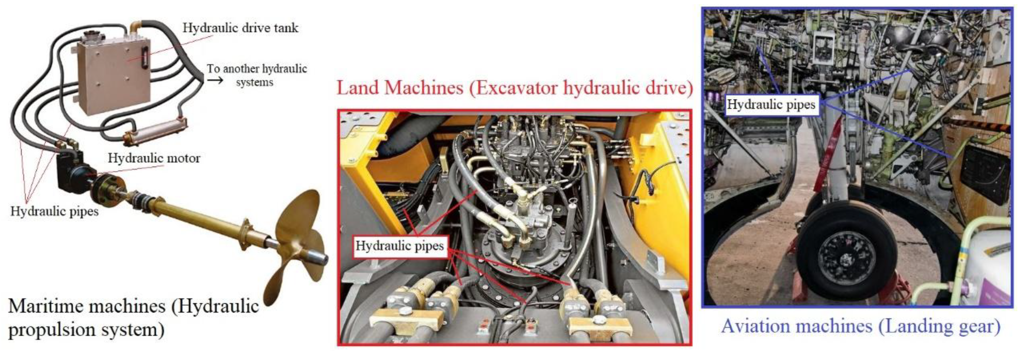
Figure 2.
Vibration spectrum of a hydraulic pipe excited by a pulsating flow of working fluid (average pressure: 5 MPa; average flow rate: 6.5 dm3/min).
Figure 2.
Vibration spectrum of a hydraulic pipe excited by a pulsating flow of working fluid (average pressure: 5 MPa; average flow rate: 6.5 dm3/min).
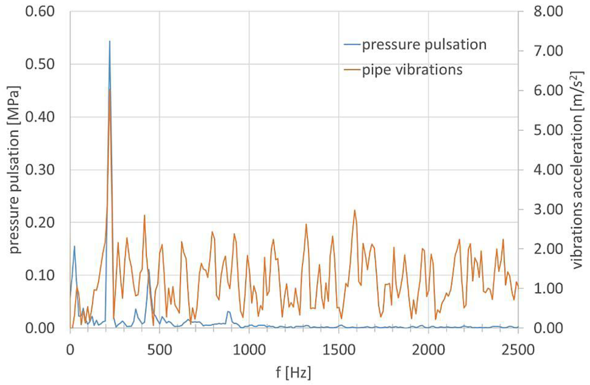
Figure 3.
Change in liquid volume in the pipe caused by an increase in system pressure under the action of the force F applied to the piston rod.
Figure 3.
Change in liquid volume in the pipe caused by an increase in system pressure under the action of the force F applied to the piston rod.
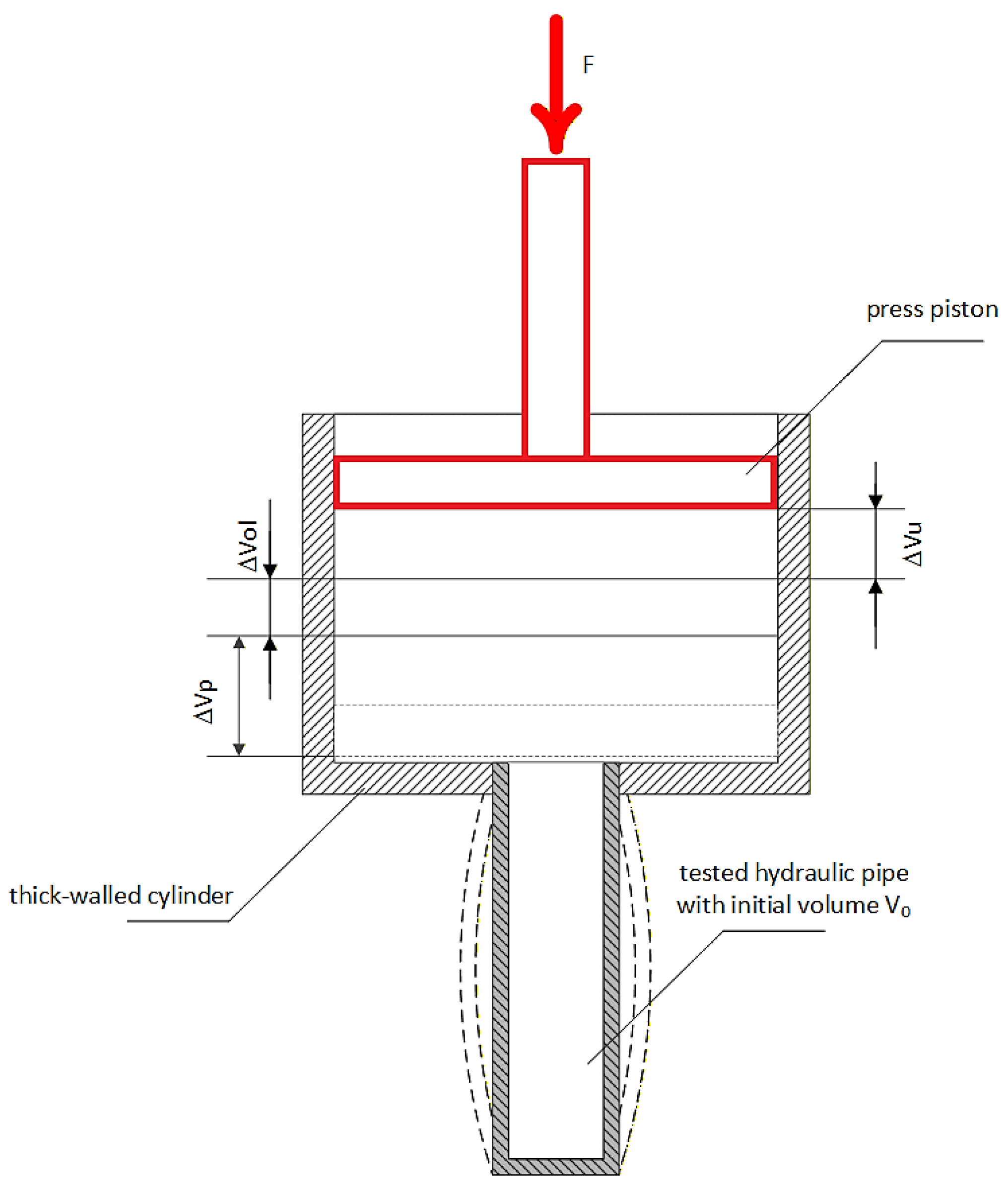
Figure 4.
Characteristics of volumetric deformations of a hydraulic pipe (filled with liquid): – experimental curve; k1 and k2 – linearisation at point B and over the range 0 – pB, respectively.
Figure 4.
Characteristics of volumetric deformations of a hydraulic pipe (filled with liquid): – experimental curve; k1 and k2 – linearisation at point B and over the range 0 – pB, respectively.
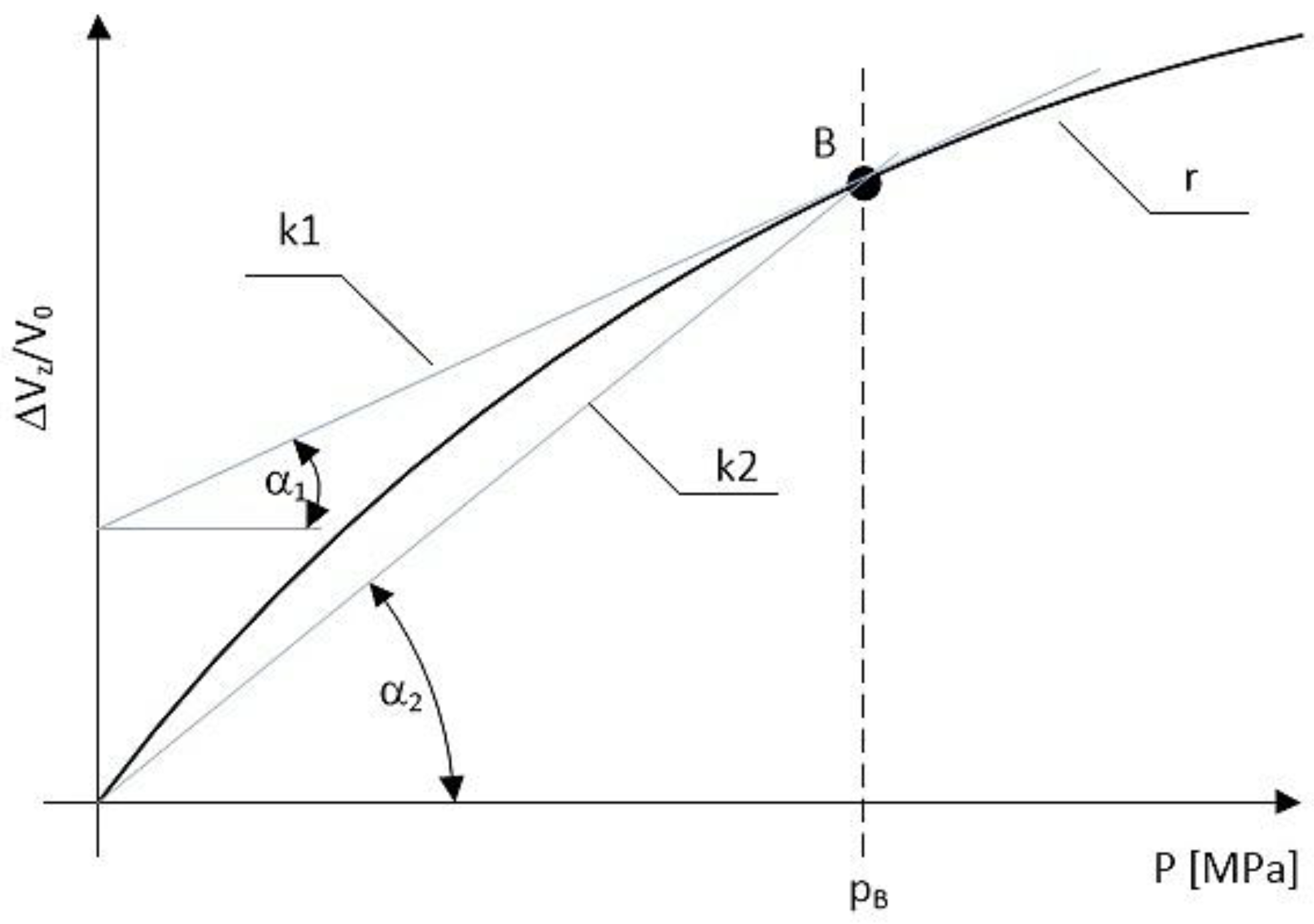
Figure 5.
Diagram of the stand for determining the substitute bulk modulus of a working fluid and a pipe: 1 – manually operated pump; 2 – measuring cylinder; 3, 5, 6, 7, 8, 9, 10, 11 – cut-off valves; 4 – pressure gauge; 12, 13, 14 – pipes under test; 15 – oil tank; 16 – thermometer.
Figure 5.
Diagram of the stand for determining the substitute bulk modulus of a working fluid and a pipe: 1 – manually operated pump; 2 – measuring cylinder; 3, 5, 6, 7, 8, 9, 10, 11 – cut-off valves; 4 – pressure gauge; 12, 13, 14 – pipes under test; 15 – oil tank; 16 – thermometer.
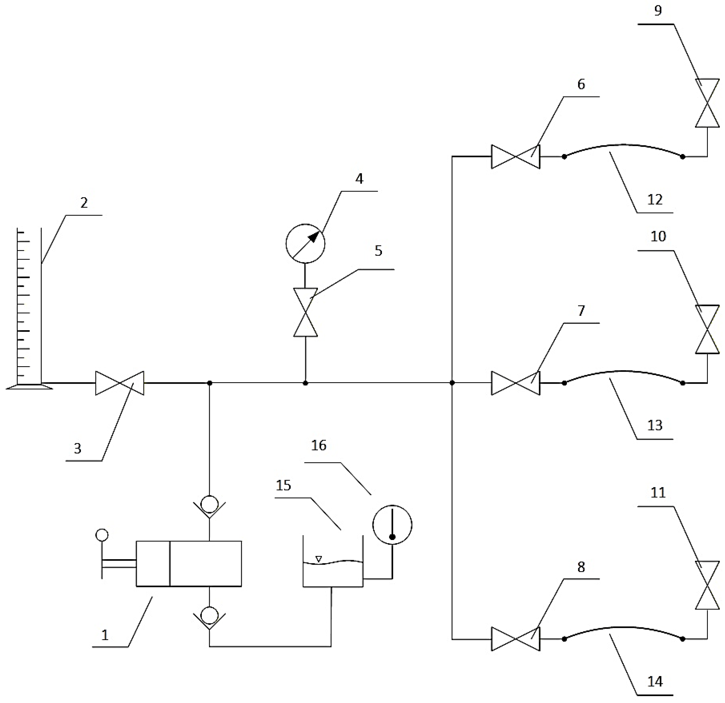
Figure 6.
Measuring station (test rig) assembled according to the described diagram.
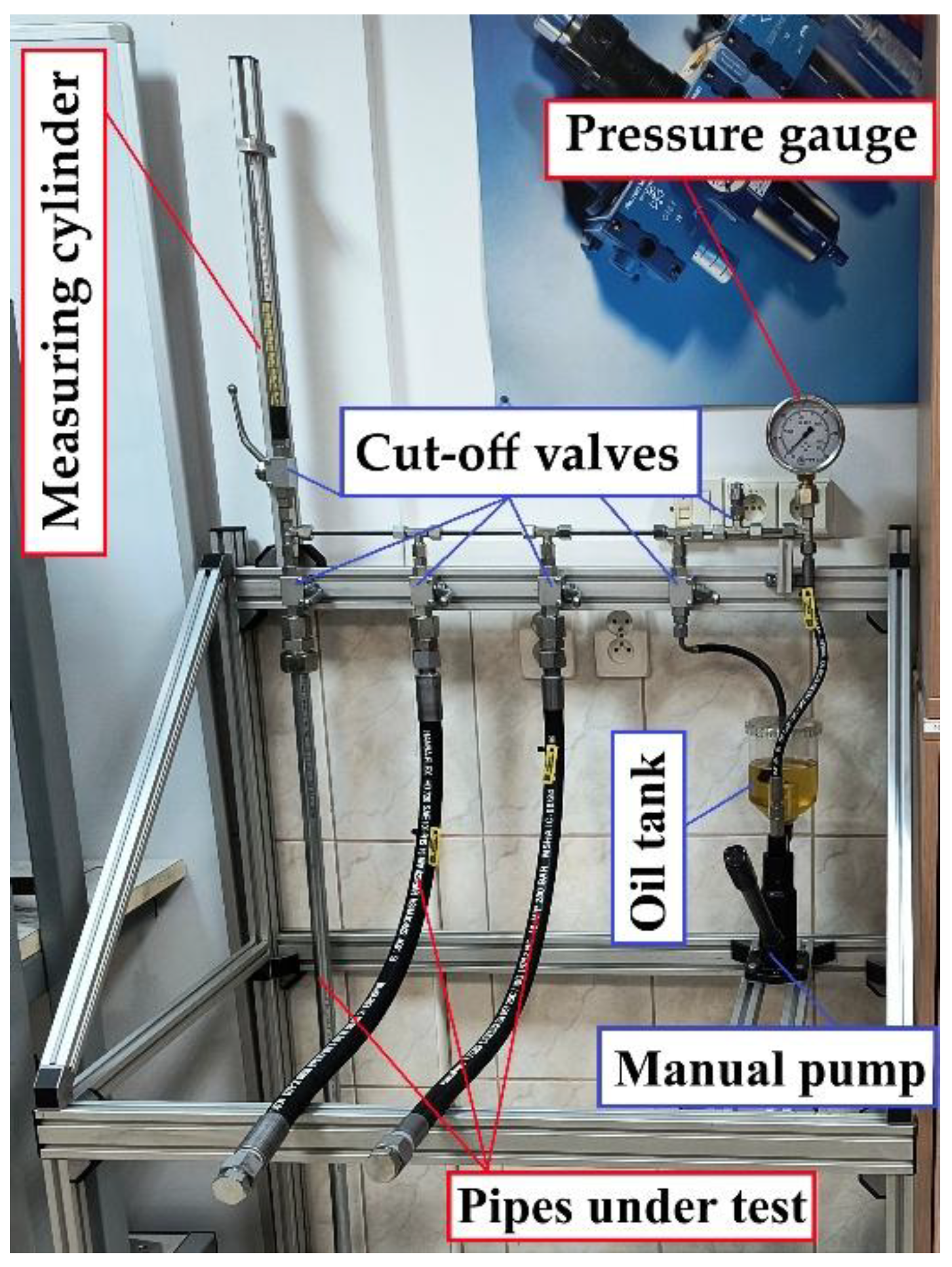
Figure 7.
Characteristics of volumetric deformations of a hydraulic pipe,
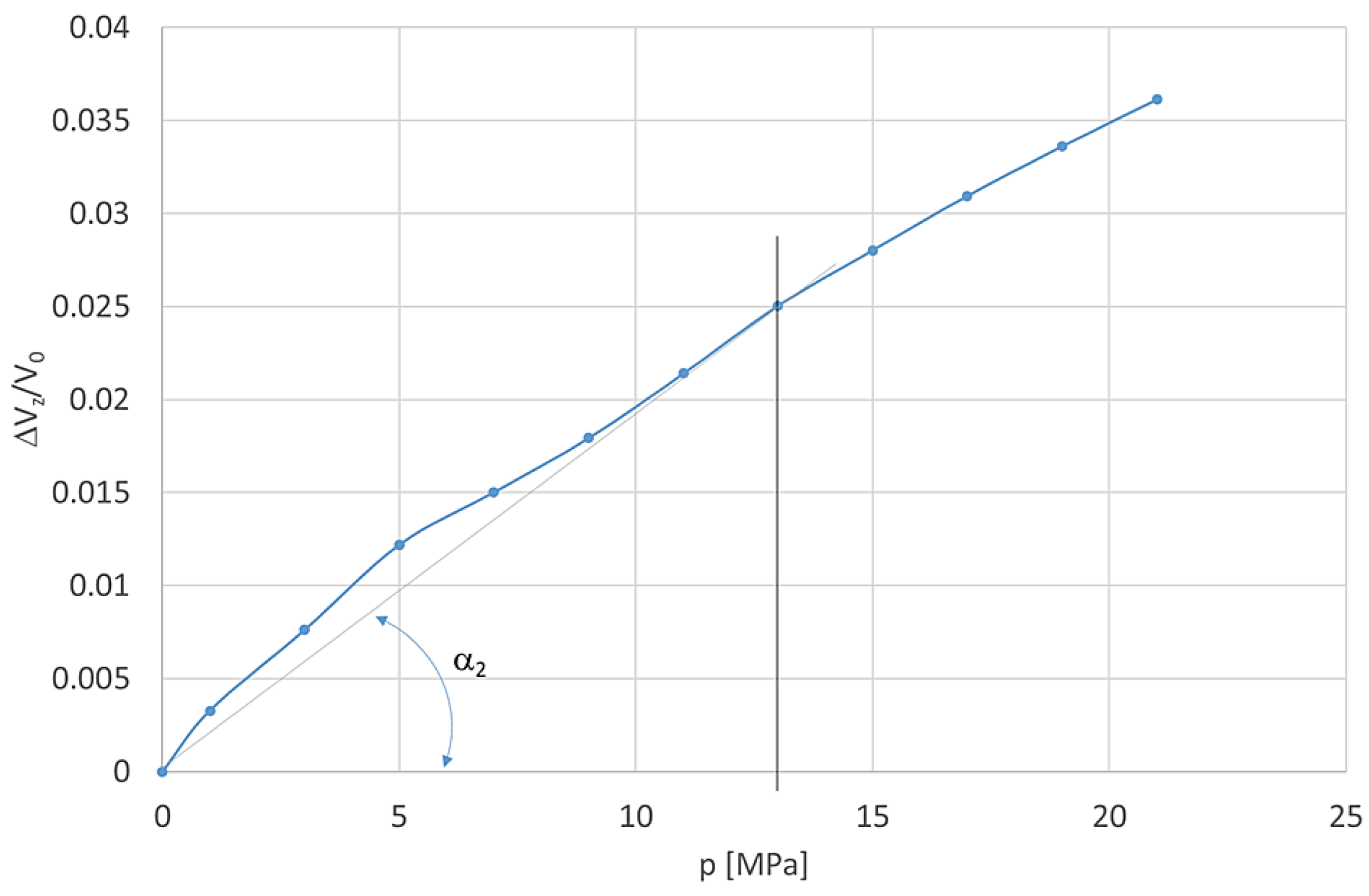
Figure 8.
Dependence of the isothermal substitute bulk modulus EzT on pressure p: 1 – steel pipe with mw = 0.167 (D = 9 mm, gp = 1.5 mm); 2 – flexible pipe with two steel braids; 3 – flexible pipe with one steel braid.
Figure 8.
Dependence of the isothermal substitute bulk modulus EzT on pressure p: 1 – steel pipe with mw = 0.167 (D = 9 mm, gp = 1.5 mm); 2 – flexible pipe with two steel braids; 3 – flexible pipe with one steel braid.
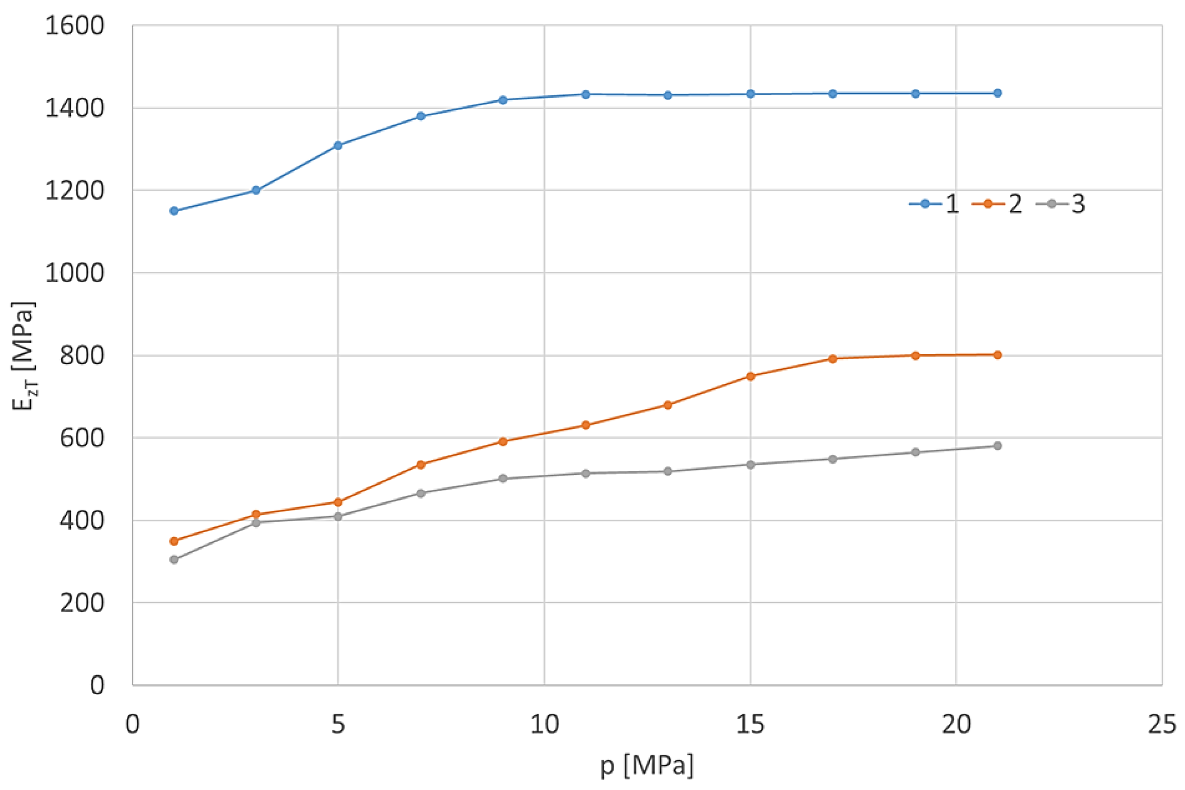
Figure 9.
Hydraulic diagram of the system for testing pressure wave propagation velocity (consisting of two parts, A and B): 1 – fixed capacity supercharging displacement pump; 2 – oil filter; 3 – supercharging unit safety valve; 4 – 1st throttle valve; 5 – variable capacity displacement pump; 6 – manovacuometer; 7 – electric motor; 8 – control pressure gauge; 9 – pressure transducer p1; 10 – pressure transducer p2; 11 – pressure transducer p3; 12 – 4/2 directional control valve; 13 – 2nd throttle valve; 14 – check valves; 15 – flow meter; 16 – safety valve; 17 – thermometer; 18 – working fluid cooler; 19 – oil tank.
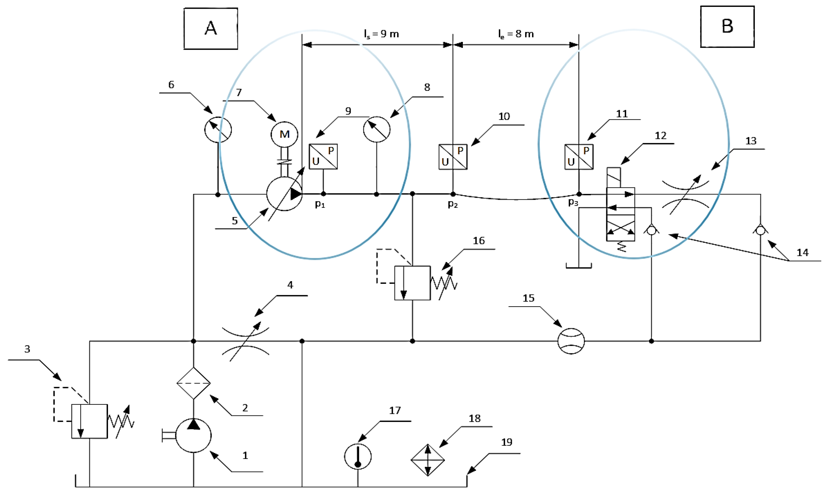
Figure 10.
Measuring stand (test rig, consisting of two parts, A and B) corresponding to the diagram for testing pressure wave propagation velocity.
Figure 10.
Measuring stand (test rig, consisting of two parts, A and B) corresponding to the diagram for testing pressure wave propagation velocity.
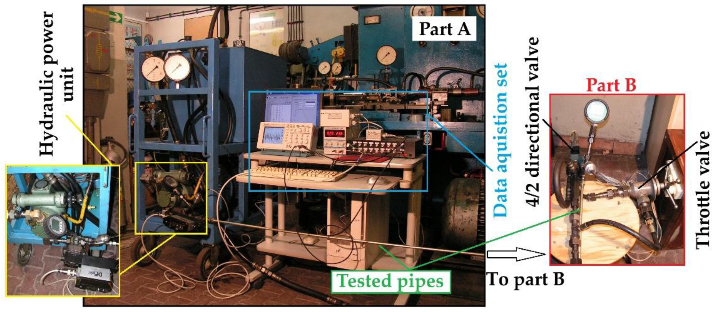
Figure 11.
Pressure curves recorded at selected points of the hydraulic circuit for an average flow rate Qav = 50 dm³/min: a – average pressure at the end of the flexible pipe, p3 = 11 MPa; b – average pressure at the end of the flexible pipe, p3 = 9 MPa; c – average pressure at the end of the flexible pipe, p3 = 4 MPa.
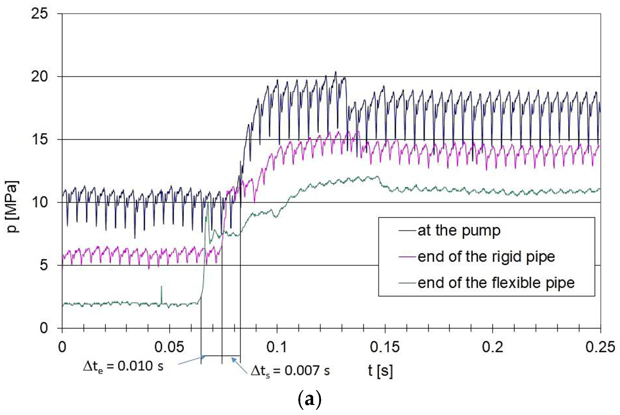
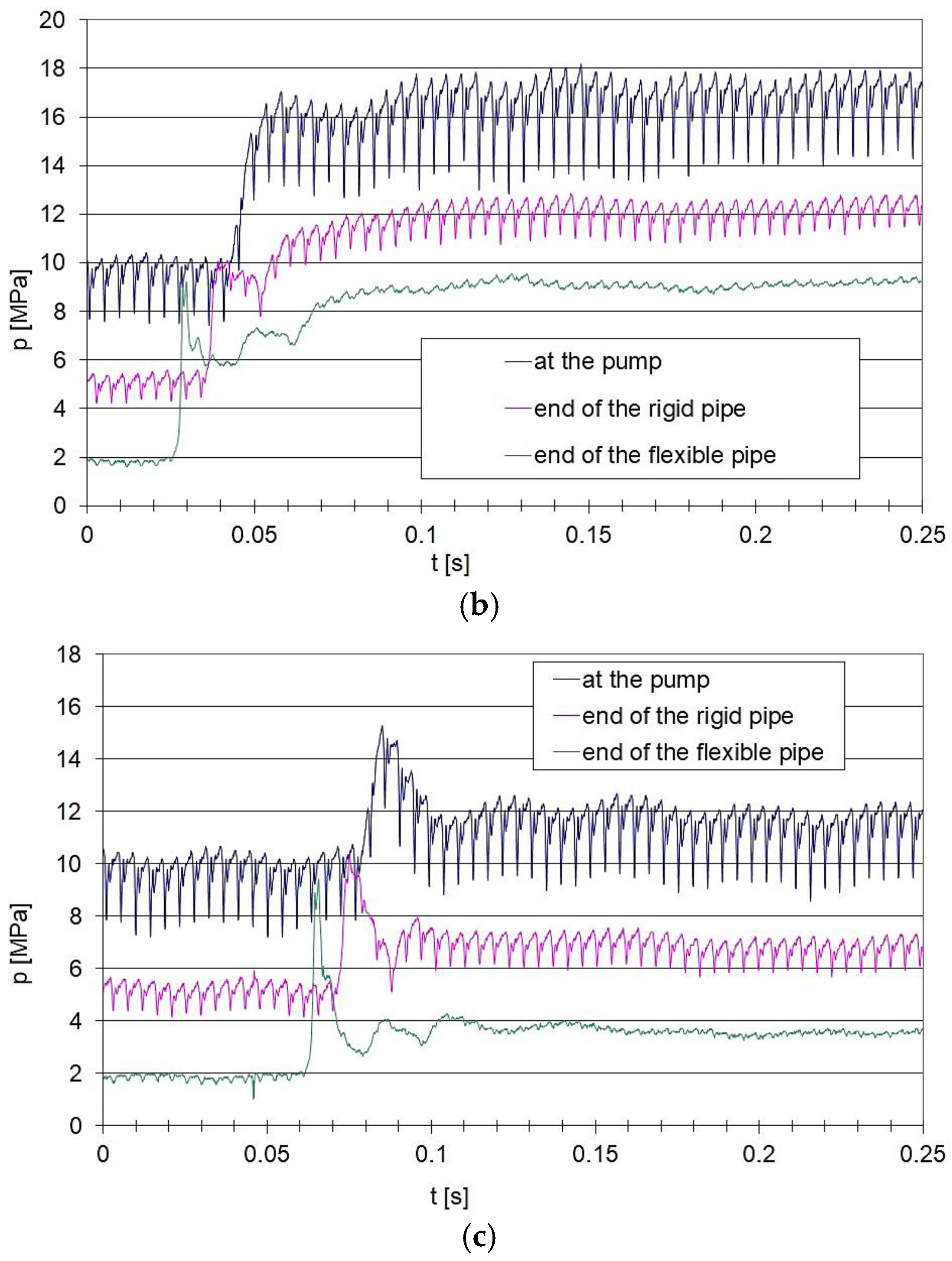
Figure 12.
Pressure curves recorded at selected points of the hydraulic circuit for an average flow rate Qav = 30 dm³/min: a – average pressure at the end of the flexible pipe, p3 = 11 MPa; b – average pressure at the end of the flexible pipe, p3 = 9 MPa; c – average pressure at the end of the flexible pipe, p3 = 4 MPa.
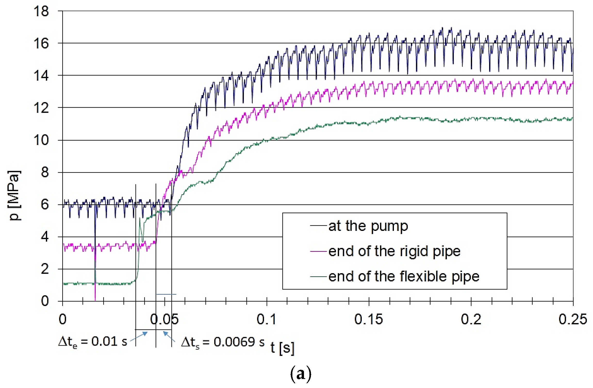
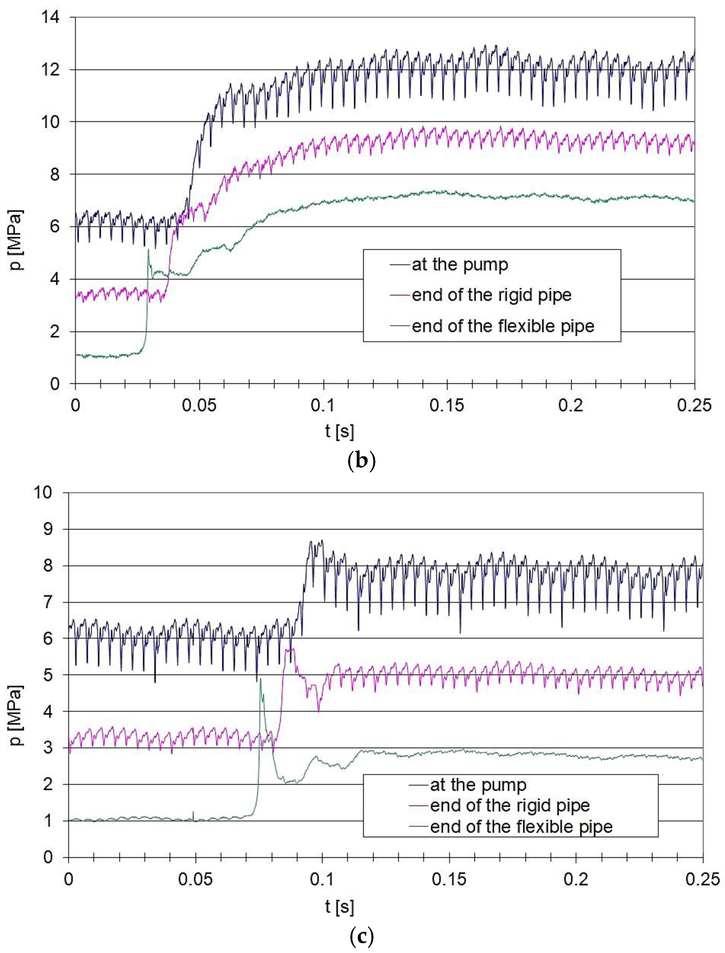
Figure 13.
Dependence of c0 on pressure along the pipeline for different pipe materials: 1 – rigid (steel) pipe; 2 – flexible pipe with two steel braids; 3 – flexible pipe with one steel braid.
Figure 13.
Dependence of c0 on pressure along the pipeline for different pipe materials: 1 – rigid (steel) pipe; 2 – flexible pipe with two steel braids; 3 – flexible pipe with one steel braid.
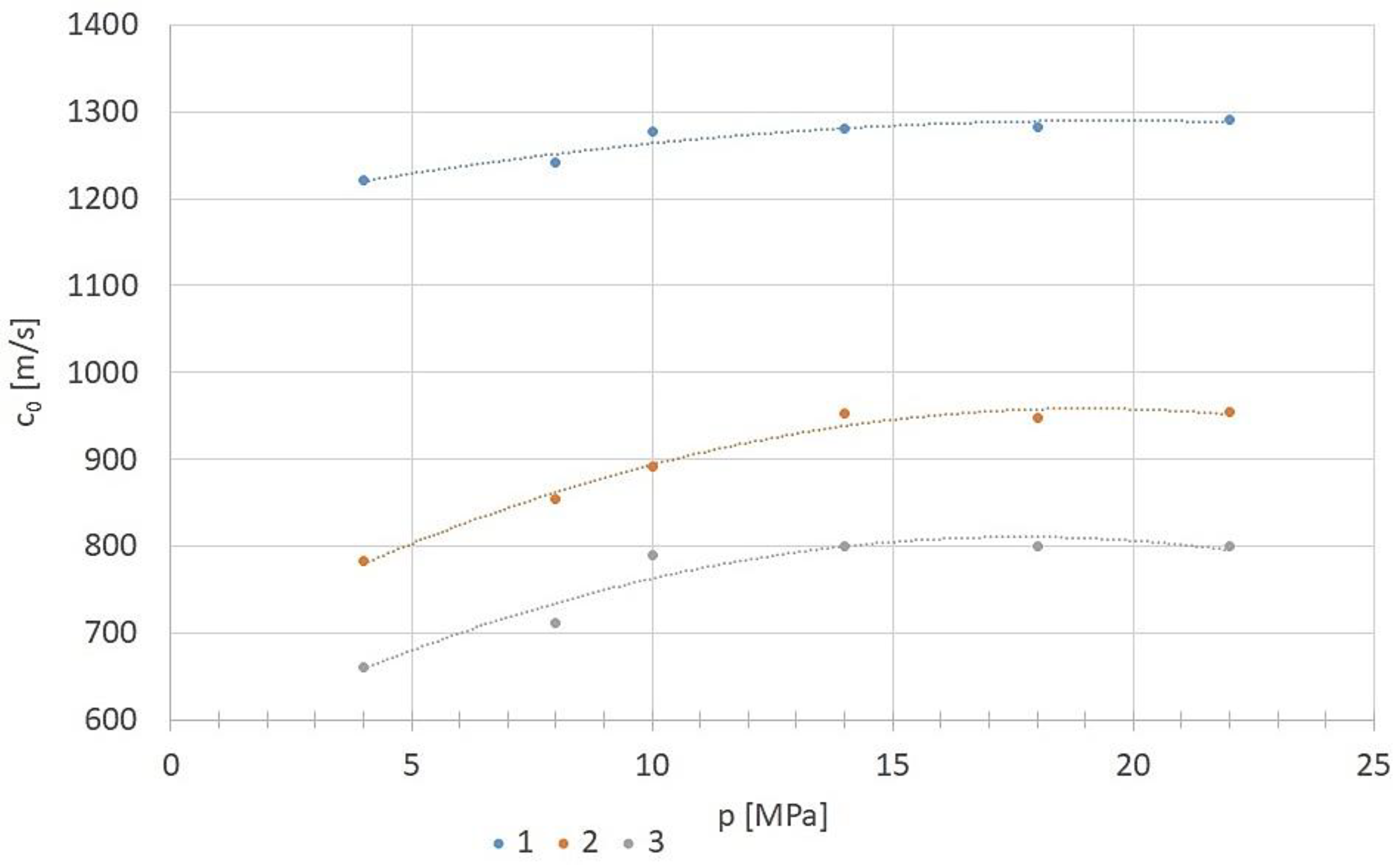
Figure 14.
Dependence of c0 on pressure inside the pipes for different pipe materials: green – rigid (steel) pipe; grey – flexible pipe with two braids; blue – flexible pipe with one braid.
Figure 14.
Dependence of c0 on pressure inside the pipes for different pipe materials: green – rigid (steel) pipe; grey – flexible pipe with two braids; blue – flexible pipe with one braid.
Disclaimer/Publisher’s Note: The statements, opinions and data contained in all publications are solely those of the individual author(s) and contributor(s) and not of MDPI and/or the editor(s). MDPI and/or the editor(s) disclaim responsibility for any injury to people or property resulting from any ideas, methods, instructions or products referred to in the content. |
© 2026 by the authors. Licensee MDPI, Basel, Switzerland. This article is an open access article distributed under the terms and conditions of the Creative Commons Attribution (CC BY) license (http://creativecommons.org/licenses/by/4.0/).
Copyright: This open access article is published under a Creative Commons CC BY 4.0 license, which permit the free download, distribution, and reuse, provided that the author and preprint are cited in any reuse.


