
Submitted:
15 April 2025
Posted:
16 April 2025
You are already at the latest version
Abstract
Pressure vessels are widely used equipment in several industries, and can operate at high pressure and temperature, which can cause major accidents in the event of a failure. The objective of this work is to analyze the behavior of longitudinal and circumferential stresses at three specific points on the wall of a pressure vessel, two distant points of geometric discontinuity (at the top and side) and one close to geometric discontinuity (at the intersection of the top and the connection) through theoretical, numerical and experimental analyses. The pressure vessel in this work is a piece of equipment used on offshore oil platforms and is part of a natural gas dehydration system. The results showed that the longitudinal and circumferential stresses at the intersection of the top and the connection were higher than the stress values at the top and side for the experimental and numerical analyses, due to the emergence of bending stresses in regions of geometric discontinuity. Another important point was the good correlation of the results between the experimental and numerical analyses using the FEM in the ANSYS software, showing that this methodology is a powerful and reliable tool in the analysis of stresses in pressure vessels.
Keywords:
Pressure Vessels
; FEM
; Geometric Discontinuity
; Stress Analysis
1. Introduction
According to Telles (2012) [1], a pressure vessel refers generically to sealed containers of any type, size, shape or purpose, with the capacity to store a pressurized fluid, whether gas or liquid. This definition includes everything from a simple pressure cooker to complex nuclear reactors. A pressure vessel is basically composed of the shell and the closing tops, both with the shapes of surfaces of revolution (cylindrical, spherical, elliptical and conical, the most common), openings for installing nozzles to connect to the piping and supports to support the equipment. Depending on the installation position, pressure vessels can be characterized as vertical, horizontal and inclined. This equipment is widely used in industrial plants in various segments, such as petrochemical, food, pharmaceutical, nuclear, chemical, sugar and alcohol, generally made of steel, with the welding process used to join the parts. According to Krüger (2014) [2], this equipment operates with pressure variations (internal pressure greater than atmospheric pressure), storing a large amount of energy inside them proportional to the operating pressure, which can be released in the event of any failure in the equipment, causing an explosion and/or leakage of flammable or toxic products. The reasons for pressure vessel failures are inadequate design, incorrect application, manufacturing, installation, maintenance, repair and operation [3].
As a result of pressure and temperature variations during pressure vessel operation, stresses and deformations are generated throughout the pressure vessel wall. However, in some regions of the wall there are geometric discontinuities that make them more critical than in other regions. According to Kharat and Kulkarni (2013) [4], openings in the walls of pressure vessels are necessary, and these openings generate geometric discontinuities that alter the distribution of stresses in the vicinity of the discontinuity, with stress values diverging from the equations of classical theory.
Analysis of stresses in pressure vessels is essential to identify the points with the highest stresses and ensure that these stresses are below the admissible design values, thus ensuring the full and safe operation of the equipment.
The stresses in a pressure vessel can be analyzed in a general way through theoretical, experimental and numerical analyses. According to Dally and Riley (1978) [5], strain gauges are the methodology used for the experimental measurement of deformations with the aim of obtaining the stresses acting on a given body. Strain gauges basically consist of a thin electrical resistance with two terminals, mounted on a support that serves as an insulator and can be made of paper or plastic resin and covered by a felt cover or the same material as the support (MELO, 2014) [6]. Strain gauges measure deformation according to the orientation of their grid, which can be uniaxial, biaxial, multiple axes or a special configuration. To measure deformations in various directions, several uniaxial strain gauges or the rosette strain gauge can be used. A rosette strain gauge is a term used for an arrangement of two or more strain gauges that are positioned at the desired location to measure along different directions of the component being measured.
For numerical analysis, the Finite Element Method (FEM) is commonly used in engineering work. Analysis using the FEM can be divided into three stages: pre-processing: defining the type of analysis, geometry, material properties, mesh and boundary conditions (loads, restrictions, types of contact, etc.); processing (or analysis): configuring the type of analysis; post-processing: obtaining the results, such as stresses, deformations, heat flux, magnetic fields, etc. Due to the importance of this component in engineering, several authors have studied the design, behavior, modeling, and simulation of pressure vessels. Niranjana et al (2018) [7] analyzed the stresses acting on a vertical pressure vessel, designed according to the sizing equations of the ASME section VIII division 1 code and by the finite element method using ANSYS software. The pressure vessel has a cylindrical body, semi-elliptical tops, connections and accessories, and specified with SA 516 GR 70 steel. For the authors, the highest stress values occur at the intersection of the connections because of the geometric discontinuities and that the accuracy of the finite element method depends on the refinement of the mesh. They concluded that the highest stress values were found around the intersection of the connection with the body.
Gonçalves (2016) [8] analyzed the stresses acting on a vertical pressure vessel (pre-evaporator), designed according to the sizing equations of the ASME section VIII division 1 code and by the finite element method using ANSYS software. The pressure vessel has a flat upper top and a torispherical lower top, a cylindrical body with an intermediate conical transition, connections and accessories, specified in SA 283 GR C steel. The authors observed that the membrane stress has higher values in the connection regions. Furthermore, they concluded that the membrane stresses in the regions distant from the geometric discontinuities and stress concentrators presented closer results when comparing the ASME equations with the finite element method, unlike the regions of greater geometric complexity, since the theory does not take into account some stresses that appear in these regions, showing the advantage of using the finite element method.
Silva (2015) [9] analyzed, using the finite element method, two vertical pressure vessel designs with the same operating conditions: one in accordance with ASME section VIII division 1 and the other in accordance with division 2. The equipment consisted of a cylindrical side, ellipsoidal tops, connections and accessories, and specified in ASTM A516 GR70 steel. For the author, pressure vessels are high-risk equipment that can cause various types of accidents, and therefore, the designs require more sophisticated computational tools that produce better results than analytical methods. He concluded that, in both designs, the stress values in the side and tops obtained by the finite element method are in accordance with the acceptance criteria for pressure vessels and that the highest stress values occurred in the change of geometry between the side and top and in the connection regions.
Kruger (2014) [10] analyzed the stress in cylindrical pressure vessel nozzles, with and without reinforcement plate, using the WRC 297 bulletin method and the finite element method using ANSYS, Nozzle Pro and SolidWorks Simulations software, and subsequently compared the results. For the author, the nozzle region has a higher probability of failure, since the opening for installing the connections causes geometric discontinuities and therefore requires special attention. He concluded that the finite element method is much more comprehensive than the WRC 297 bulletin method, since the bulletin method does not include the effect of internal pressure on the stress intensity, calculates the stress only at some specific points and has limitations regarding geometry.
Gupta (2014) [11] prepared a review of 28 studies on the design and analysis of pressure vessels, with emphasis on the factors that cause stress concentration in pressure vessels. According to the author, openings for the installation of connections in pressure vessels generate geometric discontinuities that alter the stress distribution and that equations for calculating stresses do not take these changes into account. He concluded that the ASME standard code and other codes are providing solutions for more basic cases, that the finite element method is a powerful tool for stress analysis in pressure vessels and that analyzing stress concentration in openings in pressure vessels is extremely important.
Unnava (2013) [12] designed a spherical pressure vessel with a radial connection based on ASME section VIII and analyzed it using the finite element method using ANSYS software. According to the author, the stress distribution in the region where the connection intersects with the vessel wall and the other regions will be different, since the connections cause geometric discontinuities. He concluded that stresses increase at the intersection of the vessel with the connection because of the geometric discontinuity.
Mendonça (2011) [13] analyzed the stresses of a pressure vessel, designed according to ASME section VIII division 2, by the finite element method using ANSYS software. The pressure vessel is a vertical cylindrical reactor with hemispherical tops, support, connections and accessories, specified in A-336 GR F22V steel and application of internal pressure and external forces. For the author, the search for pressure vessels with greater efficiency, higher pressure and temperature requires increasingly complex designs, which require more sophisticated computational tools to analyze their behavior. He concluded that the finite element method is a tool with great potential, as it allows the analysis of complex geometries and stress concentration points, and that for the simplest cases there is convergence with the results of the analytical formulas.
Miranda (2007) [14] analyzed the stresses acting at the intersection of the connection with a cylindrical pressure vessel with and without reinforcement plate, using the finite element method using ANSYS software. The pressure vessel was represented as a cylindrical body with radial connection, designed according to the WRC 493 bulletin, specified in Q235-A steel. Three models were developed, one without reinforcement plate, another with integral reinforcement plate and another with partially welded reinforcement, all with internal pressure application. For the author, in the region of intersection between connections and vessels, high levels of stress occur due to geometric discontinuity and that welding problems in this region can make them weaker and possibly a source of failure. He concluded that in the model without reinforcement plate, the results of the finite element method had good correlation compared to experimental and numerical analyses of another study, and that in the other two models with reinforcement plate, the stress values at the intersection of the connection with the cylindrical body of the vessel were drastically reduced.
In this context, the objective of this work is to study the behavior of the stresses acting on three specific points of the wall of a pressure vessel, two distant points of geometric discontinuity (one on the side and one on the upper cover) and one close point of geometric discontinuity (at the intersection of the upper cover with the connection), through theoretical analysis by the membrane theory and ASME Section VIII Division 2 Code Formulations [15], numerical analysis by the Finite Element Method and experimental analysis obtained in the hydrostatic test with the aid of electrical resistance extensometry.
1.1. Motivation for a Case Study
Stress analysis in pressure vessels is a relevant subject in itself, given the many studies that can be found in the literature. Its relevance is due to the fact that pressure vessels are widely used in various industries, and any failure can cause major accidents. Therefore, identifying the most critical points, where stresses are higher and above the permissible stresses, allows us to obtain safer, more reliable and economically more viable equipment.
Two situations can be mentioned that add relevance to this work: the location of the equipment and the performance of the experimental analysis. The equipment targeted by this work is part of a gas dehydration system installed on an offshore platform, which can only be accessed by boat or helicopter. Therefore, any failure that requires repair at the factory or replacement of the equipment after it has been installed would be highly costly due to restricted access. Many studies found in the literature analyze the stresses in pressure vessels designed based on design standards or codes, mainly the ASME code, through numerical analysis using the finite element method, and therefore the performance of the experimental analysis adds relevance to this work. The experimental analysis performed occurs with the hydrostatic test of the equipment after its manufacture, which is subjected to twice its normal operating pressure.
2. Materials and Methods
The methodology adopted for this work consisted of the following steps, which are shown and summarized in Figure 1:
1) performing a hydrostatic test on the equipment and obtaining the deformation values at three specific points (side, top cover and intersection of the top cover with the connection) using electrical resistance strain gages during pressure vessel pressurization; converting the deformation values found in the hydrostatic test into stress values using experimental calculations based on the stress-deformation relations.
2) applying the membrane theory formulas and ASME Section VIII Division 2 Code formulations [15] according to the equipment design specifications and obtaining the stresses at three specific points for the same pressures as the hydrostatic test.
3) developing a computational model for the pressure vessel considered in this work and obtaining the stresses at three specific points for the same pressures as the hydrostatic test using the finite element method in ANSYS software.
2.1. Equipment
The pressure vessel analyzed in this work is custom-made equipment, according to its operating characteristics and application within the production process. In this case, all the design, manufacturing, inspection, testing and installation of the equipment followed NR13 and the ASME code section VIII division 2 [15]. Figure 2 shows an overview of the equipment with its main parts: upper and lower covers, side, support skirt, connections and accessories. Table 1 presents some basic information about the equipment according to the manufacturer's specifications and also data that is used in the calculations of stresses in the various analyses.
2.2. Hydrostatic Test
The hydrostatic test aims to detect possible defects, failures or leaks in any part of the equipment, and consists of filling with water or another liquid until all the air is removed and slowly pressurized to a certain pressure called the hydrostatic test pressure. It is desirable that the hydrostatic test pressure be as high as possible, respecting the safety of the least resistant parts, and always higher than the design pressure and maximum permitted working pressure.
According to ASME section VIII division 2 [15], the hydrostatic test pressure (PT) is calculated as the larger value between Equations 1 and 2.
where:
PT =1,43 x MAWP
PT = 1,25 x MAWP x LSR
MAWP – Maximum Allowable Working Pressure
LSR – Lowest Stress Ratio
LSR is the ratio ST / S where ST is the allowable stress at the test temperature and S is the allowable stress at the design temperature, and is calculated for each part of the pressure vessel except bolting. Regarding the allowable stresses for the hydrostatic test, the ASME section VIII division 2 code [15] establishes some conditions according to Equations 3, 4 and 5.
where:
Pm ≤ (0.95 x Sy)
Pm + Pb ≤ (1.43 x Sy) for Pm ≤ (0.67 x Sy)
Pm + Pb ≤ (2.43 x Sy – 1.5 x Pm) for (0.67 x Sy) < Pm ≤ (0.95 x Sy)
Pm – overall primary membrane stress
Pb – primary bending stress
Sy – yield stress
According to the ASME section VIII division 2 code [15], the longitudinal and circumferential membrane stresses of the cylindrical side subjected only to internal pressure can be calculated using Equations 6 and 7.
According to ASME section VIII division 2 [15], the longitudinal and circumferential membrane stresses of hemispherical tops subjected only to internal pressure can be calculated using Equation 8:
where:
σlong – longitudinal membrane stress
σcirc – circumferential membrane stress
P – internal pressure
D – internal diameter
D0 – external diameter
WE – welded joint efficiency
The minimum hydrostatic test pressure was calculated as explained above, with the value found being 14.66 MPa, according to ASME section VIII division 2 code and Equation 1, but the hydrostatic test pressure applied was 15 MPa. This pressure is more than double the normal working pressure specified in the project, which is 7.36 MPa. The hydrostatic test was performed horizontally.
With the pressure vessel positioned at the hydrostatic test site, preparation for the hydrostatic test began by closing all connections to the respective flanges. The water inlet valve was installed on one of the flanges, which was connected to a positive displacement hydraulic pump, responsible for pressurizing the equipment. The pressure gauge was installed on another flange to monitor the pressure variation inside the equipment. After installing all flanges, the equipment was filled with water. The three specific points for obtaining the data were prepared through the sanding process for better adhesion of the strain gauges to the surface. The gluing of the strain gauges followed the manufacturer's standard procedure. The strain gauges used are of the rectangular rosette type and are from the KYOWA brand: KFG – 5 –120 – D17 – 23, Gage Factor: 2.12 ± 1.0%, Gage Length: 5 mm. Figure 3 shows images of the assembly.
After all preparation, the hydrostatic test of the pressure vessel was performed. The internal pressure of the equipment was varied from 0 to 15 MPa, with the deformation values measured every 0.1 second and captured by an HBM® Quantumx MX1615 signal conditioner. Approximately 2,603 seconds (approximately 44 minutes) elapsed to reach the pressure of 15 MPa. Each rectangular rosette strain gauge generated three deformation values, therefore 9 deformation values were generated every 0.1 second, totaling approximately 234,270 deformation values. The times were recorded for every 0.5 MPa variation from 0 to 15 MPa, making it possible to know the deformations for multiples of 0.5 MPa in all strain gauges, thus totaling 270 deformation values.
After performing the hydrostatic test and obtaining the deformations at the three specific points, the next step was to convert the deformations into maximum (σ1) and minimum (σ2) principal stresses, which coincide with the circumferential (σcirc) and longitudinal (σlong) stresses, using Equations 9 and 10.
where εt and εl mean, respectively, transverse deformation and longitudinal deformation.
The values of the constants E and ν were taken from Table 1 and the deformation values obtained with the extensometers.
2.3. Theoretical Calculation of Stresses Using Membrane Theory
Theoretical calculations were applied to the three specific points of the hydrostatic test to calculate the longitudinal and circumferential stresses acting according to the variation in internal pressure in the equipment. The hydrostatic pressure caused by the water column on the walls of the equipment was not considered in both theoretical calculations, since the maximum value of the hydrostatic pressure is much lower than the values of the internal pressure applied to the equipment.
The theoretical calculation of the longitudinal and circumferential stresses for the side follows in accordance with Equations 11 and 12:
Equation 13 allows the theoretical calculation of the longitudinal and circumferential stresses for the upper top.
The internal pressure values ranged from 0.5 to 15 MPa, while the internal radius and thickness values were considered respectively 1350 mm and 99 mm for the side and 1357 mm and 50 mm for the top.
2.4. Theoretical Calculation of Stresses Using ASME Code Formulations
To calculate the stresses using the ASME code formulations, Equations (6), (7) and (8), presented above, were used. The internal pressure values ranged from 0.5 to 15 MPa, the welded joint efficiency was considered 1 (according to the design), while the internal radius and thickness values were considered respectively 1350 mm and 99 mm for the side and 1357 mm and 50 mm for the top. After substituting these values in Equations (6), (7) and (8), the analysis results by the ASME code formulations can be obtained and will be shown below.
2.5. Numerical Analysis
The ANSYS software was used to perform the numerical analysis using the finite element method. The entire modeling stage was developed using the SPACECLAIM software that accompanies the aforementioned software version.
Each component of the equipment was modeled independently as a solid element, and after modeling all components, the equipment was assembled, as shown in Figure 4(a).
To optimize the simulation of the pressure vessel, the complete model of the equipment in Figure 4(a) had its geometry simplified to only the essential parts of the study of this work, Figure 4(b), using the simplified model. Since the objective of this work is to analyze the behavior of the stress at three specific points of the equipment, which are located on the side, upper cover and intersection of the upper cover with the connection, these components were kept in the simplified model in addition to the lower cover and the connection cover.
Other considerations in the simplified model were adopted in relation to the original design of the pressure vessel:
- the wall of the upper lid has a thickness of 47 mm plus 3 mm of corrosion coating, however in the model the wall of the upper lid was modeled with a thickness of 50 mm to maintain the agreement of the transition from the side to the upper lid;
- the wall of the side is divided into two parts connected by a circumferential weld, with one part having a thickness of 96 mm plus 3 mm of corrosion coating and the other part having a thickness of 99 mm, however in the model the entire wall of the side was modeled as a single piece with a thickness of 99 mm;
- no welds were represented in the simplified model.
In summary, in the model used for the evaluation using the finite element tool, these are only the elements where the experimental stresses were taken. In addition, the locations that specifically require corrosion protection were considered as an element. In this way, the stresses obtained can be compared with the experimental stresses, since the subtraction of elements does not influence the evaluation, since they are far from the evaluated elements.
The steels used in the pressure vessel analysis were created based on the structure steel material from the ANSYS library, with changes only in the following properties according to projects and standards:
- SA 516 grade 70
Yield stress: 38 ksi (262 MPa)
Rupture stress: 70 ksi (482 MPa)
- SA 350 lf2 class 1
Yield stress: 36 ksi (248 MPa)
Rupture stress: 70 ksi (482 MPa)
- Poisson's ratio equal to 0.3 and modulus of elasticity equal to 200 GPa.
2.5.1. Stress Linearization
The analysis by the finite element method in the ANSYS software, through stress linearization, allows the decomposition of the stress acting along the thickness of the pressure vessel wall into membrane, bending and peak stress for models developed as solid elements, which is the case of this work.
Stress linearization can be applied on a stress classification line (SCL) or on a stress classification plane (SCP). In this work, the stress classification line was applied. According to Figueiredo (2021) [16], stress classification lines are the paths chosen by the analyst to linearize and separate the real stress distribution obtained into membrane and bending stresses.
Stresses are generally non-linear, but along this line the stresses are linearized to obtain the membrane and bending stresses. Membrane stresses are constant throughout the wall thickness, while bending stresses are linear [17].
To facilitate the application of stress linearization, the section of the side and top was performed in planes that contained the three specific points that would be analyzed by the finite element method in the ANSYS software. These planes sectioned the side and top passing through the central axis of each component. Figure 5 shows the three planes, with the plane highlighted in blue being the plane that sections the side and the other two planes that section the top.
2.5.2. Mesh Generation
There was a differentiation in the mesh for some components of the pressure vessel that were more important, such as the side, the upper lid and the connection. To create this differentiation in the mesh, the body sizing option was used, in which the size of the mesh element is determined. The pressure vessel was divided into three parts and body sizing was applied to each part, determining a different element size for each of the three parts.
- -
- side: element size equal to 0.2 m
- -
- upper lid and connection: element size equal to 0.08 m
- -
- connection cover, lower lid and supports: element size equal to 0.4 m
After applying body sizing, the mesh was generated with 29,799.0 nodes and 7,315.0 elements in total. Figure 6 shows the ANSYS Element Quality metric graph for the model mesh of this work. A convergence study was performed to establish the accuracy of the numerical model. Sequential refinements were used in this study. The results indicate that the accuracy is better than 0.5%.
3. Results
3.1. Hydrostatic Test
Figure 7 and Figure 8 (a) and (b) show the graphs of the longitudinal and circumferential (transversal) stresses for the points located on the top cover, on the side and intersection using membrane theory and ASME code formulations, respectively, Obtained from Equations (6) – (8). Comparing the stress values shown in the Figures and the Equations for calculating them, the values are the same, since both specific points belong to the top cover and the formulas for calculating the longitudinal and circumferential stresses are the same, with no differentiation for points close (intersection) or far (top cover) from geometric discontinuity. Figure 7(b) shows that the stress for the top cover and the intersection are identical, so a point was extrapolated to 15.5 MPa to identify the black curve - Top cover and verify that it is below the red curve. Furthermore, it can also be seen that for the point located at side the stress curve is close to the curve for the top cover and the intersection.
The graphs in Figure 7 reflect, in relation to the membrane theory, that for circumferential stress, there is uniformity of the stress curve due to the symmetry of the pressure vessel. Since the stress at the intersection and at the top is calculated based on the equations of a spherical vessel, this uniformity of values is obtained. Now, for the longitudinal stresses, uniformity is observed for the top and the intersection, as they are points located in the spherical part, where there is a single stress, differentiating it from the longitudinal stress calculated in the body of the pressure vessel.
Figure 8 shows the same effect, the curves of the intersection and top cover points are superimposed, and only the blue curve of the intersection point can be seen. But this happens because the calculated voltages are the same.
The results shown in Table 2, Table 3 and Table 4 represent the deformation values obtained at the specific points where the strain gauges were glued, namely, the side, the top cover and at the intersection of the top cover with the connection, which is in a region close to the geometric discontinuity. From the data obtained, using Equations 9 and 10, the longitudinal and circumferential (transversal) stress values were obtained for each specific point. The stresses are shown graphically in Figure 9.
3.2. Experimental Analysis
By applying the experimental methodology, Equations 9 and 10, and the information obtained in Table 2, Table 3 and Table 4, the results of the longitudinal and circumferential/transversal (experimental) stresses shown in Figure 9(a) and (b) were obtained.
When comparing the values of the longitudinal and circumferential/transversal stresses of the upper lid and the intersection of the upper lid with the connection, it was observed that the values of the intersection are greater than the values of the top, on average 41% for the longitudinal stress and 56% for the circumferential/transversal stress. According to the membrane theory, the stress values in the upper lid and intersection should be equal, since both points belong to the upper lid (same internal radius, thickness and internal pressure applied), with only the membrane stress existing and disregarding the bending stress along the thickness of the pressure vessel wall. However, in practice, the experimental analysis showed that in the intersection of the upper lid with the connection, which is located close to a geometric discontinuity, the bending stresses have considerable values and that they are not taken into account by the membrane theory and ASME code formulation.
3.1. Finite Element Method in ANSYS Software
3.1.1. Stresses at Three Specific Points
By applying the methodology of Item 2.4, the numerical analysis was performed to obtain the longitudinal and circumferential stresses using the finite element method in the ANSYS software. A simulation was performed for the same theoretical and experimental data. The results are shown in the graphs of Figure 10(a) and (b).
When comparing the values of the longitudinal and circumferential stresses of the upper cover and the intersection of the upper cover with the connection, it is observed that the values of the intersection are greater than those of the cover, on average 15% for the longitudinal stress and 39% for the circumferential stress. According to the membrane theory, the stress values in the upper cover and intersection should be equal, since both points belong to the upper cover (same internal radius, thickness and internal pressure applied), with only the membrane stress existing and disregarding the bending stress along the thickness of the pressure vessel wall. However, the analysis by the finite element method showed that in the intersection of the upper cover with the connection, which is located close to a geometric discontinuity, the bending stresses have considerable values and are not taken into account by the membrane theory.
Since the circumferential stress value was greater than the longitudinal stress at the hydrostatic test pressure of 15 MPa for the three points under study, a more detailed analysis will be presented at the three points evaluated, through finite element simulation using ANSYS software.
3.1.2. Side
On the side, the circumferential stress has a minimum value of 112.84 MPa and a maximum value of 244.62 MPa. The highest circumferential stress values occur in the region of the supports and the connection of the side to the upper top, as shown in Figure 11 (a). Figure 11 (b) shows a mapping of the circumferential stress at several external points on the side of the side. From the mapping, it can be seen that the circumferential stress has higher values on the left side of the figure, where the side is connected to the upper top, which is a region of geometric discontinuity. The intersection of the side with the lower top, which is also a region of geometric discontinuity, which occurs on the right side of the figure, has the lowest values of circumferential stress. It can also be seen that the circumferential stress increases in value from the upper part of the side to the central region, and then decreases again. The values are in Pa.
In Figure 11(a) and (b) you can see regions in yellow. These apparent inconsistencies actually reveal the action of the loads in the operation of the equipment. During the hydrostatic test, there is not only pressure, but also the weight of the water and the reactions of the supports that support the vessel. This implies interference in the load path, even though it is a homogeneous distribution and far from the stress concentrator points. Furthermore, when comparing the simulated and analytical results, it is observed that the results are close.
3.1.3. Top Cover
Figure 12 (a) shows how the circumferential stress behaves only in the upper cover, with a minimum value of 189.67 MPa and a maximum of 323.59 MPa. The highest circumferential stress in the upper cover occurred at the outer edge of the connection opening, close to a geometric discontinuity. In this analysis, it can be seen that the maximum circumferential stress of 323.59 MPa exceeds the yield stress of the material, however, in the tests performed, twice the working pressure is used, and according to the ASME VIII division 2 standard, this stress extrapolation is momentary, characteristic of the test and that for normal operating conditions this does not occur, according to the stress indices shown, therefore there is no need to evaluate the element in the plastic state. Figure 12 (b) shows a mapping of the circumferential stress at several external points of the upper cover. The mapping shows that the circumferential stress has higher values at the connection opening, which is a region of geometric discontinuity, decreases in the central region and increases again when approaching the connection between the upper cover and the side, which is also a region of geometric discontinuity. Values in Pa.
3.1.4. Pressure Vessel
Figure 13 (a) shows how the circumferential stress behaves throughout the pressure vessel, with a minimum value of -12.908 MPa and a maximum of 364.59 MPa. The greatest circumferential stress throughout the pressure vessel at a pressure of 15 MPa occurs at the connection wall, a region of geometric discontinuity. As observed in Figure 13(b).
Figure 13(a) and (b) show the simulation of the pressure vessel in operation. This simulation is in line with the theory, showing higher stresses at the top discontinuity. Geometric discontinuities are found in the walls of pressure vessels, which consist of variations in thickness, openings for accessories, shape transitions, misalignments and joints of parts of the vessel, such as, for example, side with top or top with connection. When a load is applied to the pressure vessel, for example, internal pressure, the pressure vessel as a whole deforms, however, in the regions of geometric discontinuity, adjacent elements deform in different ways, even though they form a continuous structure. There are bending moments in the transition region of the two geometries, thus generating bending stresses. Considering the joint of the top with the side of a generic pressure vessel, subjected to internal pressure, each element, top and side, tend to move differently, generating forces and moments at the joint that cause bending stresses. These bending stresses imply an increase in normal stress in these discontinuity regions.
Since the hydrostatic test does not only present pressure as a stress, but also the weight of the water and the reactions of the supports that support the vessel, this implies an interference in the load path. In this work, a homogeneous distribution was obtained, far from the stress concentrator points. Furthermore, when comparing the simulated results with the analytical ones, the results obtained are close, showing the efficiency of the model.
4. Discussion
The stress values from the theoretical analysis were chosen as a reference and compared with the others, it can be seen in Table 5, with the values analyzed from the pressure of 3 MPa for the side, upper cover and intersection.
When comparing the experimental and simulation results with the theoretical results, it is observed that the results from the simulation using ANSYS software were close to the theoretical results, diverging slightly at the intersection, where the equations are unable to translate the influence of the discontinuity, requiring an analysis with a stress concentrator. In fact, according to the membrane theory, the flexural and torsional stiffnesses in the shell should not be considered, which causes the bending and torsional moments to be zero. Under these conditions, the shear forces are also nullified and the shell will be stressed solely by normal and tangential forces. The ASME code takes these factors into consideration, therefore, it is essential to evaluate them in a pressure vessel design by extensometry and finite element modeling and simulation. The bending effect intensifies stresses in regions close to geometric discontinuities, which is why these are regions with a greater probability of failure. The theoretical equations defined by membrane theory have limitations in their application in regions of the pressure vessel with geometric discontinuities, due to bending stresses. The simulation analysis can already see this worsening in the stress, which was more evident in the circumferential stress. The experimental results were all below the theoretical stress, showing that the stresses present in the vessel are lower than the stresses for which they were designed, except at the intersection, where there is a geometric discontinuity, which increases the stress at that point. Wadkar et al. (2015) [18] in their study using FEM and pressure vessels, managed to validate the model when the stresses obtained were close to the theoretical stresses, calculated by more than one equation.
4.1. Mises Tension Consolidation
In order to analyze the consolidation of the stresses from the 4 analyses, it was necessary to convert the longitudinal and circumferential stresses from the theoretical, ASME and experimental analyses into equivalent Von Mises stress using Equation 14 to calculate the equivalent stress in a plane stress state.
where σeq is Von Mises equivalent stress, σ1 is maximum principal stress and σ2 is minimum principal stress.
The stresses obtained by the experimental analysis at the three specific points were obtained on the external surface of the pressure vessel wall. Based on the values obtained from the Von Mises equivalent stress in the FEM analysis on the internal and external surfaces at the three specific points, it was possible to project the value of the Von Mises equivalent stress on the internal surface of the experimental analysis using the percentage of variation between the internal and external values of the FEM analysis.

Table 6.
shows the consolidated Von Mises equivalent stress values for the side.
| Experimental Stress | Theoretical Stress | ASME Stress | FEM Stress | ||||
|---|---|---|---|---|---|---|---|
| Pressure (MPa) | Internal Projection (MPa) | External (MPa) | (MPa) | (MPa) | Internal (MPa) | External (MPa) | |
| 0.5 | 0.90 | 2.69 | 5.90 | 5.91 | 4.04 | 12.01 | |
| 1.0 | 3.41 | 7.71 | 11.81 | 11.81 | 7.84 | 17.72 | |
| 1.5 | 6.90 | 11.65 | 17.71 | 17.72 | 13.88 | 23.44 | |
| 2.0 | 11.63 | 16.75 | 23.62 | 23.62 | 20.25 | 29.18 | |
| 2.5 | 17.53 | 22.91 | 29.52 | 29.53 | 26.71 | 34.91 | |
| 3.0 | 23.63 | 28.92 | 35.43 | 35.44 | 33.21 | 40.65 | |
| 3.5 | 29.15 | 34.03 | 41.33 | 41.34 | 39.74 | 46.39 | |
| 4.0 | 34.64 | 39.02 | 47.24 | 47.25 | 46.28 | 52.13 | |
| 4.5 | 40.20 | 44.04 | 53.14 | 53.15 | 52.82 | 57.87 | |
| 5.0 | 45.47 | 48.71 | 59.05 | 59.06 | 59.37 | 63.61 | |
| 5.5 | 51.36 | 54.03 | 64.95 | 64.97 | 65.92 | 69.35 | |
| 6.0 | 57.22 | 59.30 | 70.86 | 70.87 | 72.47 | 75.10 | |
| 6.5 | 64.82 | 66.30 | 76.76 | 76.78 | 79.03 | 80.84 | |
| 7.0 | 70.82 | 71.65 | 82.67 | 82.68 | 85.58 | 86.59 | |
| 7.5 | 76.12 | 76.28 | 88.57 | 88.59 | 92.14 | 92.33 | |
| 8.0 | 80.52 | 80.02 | 94.48 | 94.50 | 98.70 | 98.08 | |
| 8.5 | 85.53 | 84.37 | 100.38 | 100.40 | 105.25 | 103.82 | |
| 9.0 | 91.86 | 90.02 | 106.28 | 106.31 | 111.81 | 109.57 | |
| 9.5 | 96.84 | 94.33 | 112.19 | 112.21 | 118.37 | 115.31 | |
| 10.0 | 102.40 | 99.23 | 118.09 | 118.12 | 124.93 | 121.06 | |
| 10.5 | 107.58 | 103.75 | 124.00 | 124.02 | 131.49 | 126.81 | |
| 11.0 | 111.82 | 107.36 | 129.90 | 129.93 | 138.05 | 132.55 | |
| 11.5 | 117.66 | 112.53 | 135.81 | 135.84 | 144.61 | 138.30 | |
| 12.0 | 124.07 | 118.22 | 141.71 | 141.74 | 151.17 | 144.05 | |
| 12.5 | 129.95 | 123.42 | 147.62 | 147.65 | 157.72 | 149.79 | |
| 13.0 | 136.25 | 129.00 | 153.52 | 153.55 | 164.28 | 155.54 | |
| 13.5 | 141.32 | 133.42 | 159.43 | 159.46 | 170.84 | 161.29 | |
| 14.0 | 146.44 | 137.89 | 165.33 | 165.37 | 177.40 | 167.04 | |
| 14.5 | 153.06 | 143.76 | 171.24 | 171.27 | 183.96 | 172.78 | |
| 15.0 | 158.37 | 148.40 | 177.14 | 177.18 | 190.52 | 178.53 | |
In Table 7, the values of the von-Mises equivalent stress in the experimental analysis are below the values of the theoretical and ASME analysis, while the values of the FEM analysis on the inner surface are above. The same analysis was performed for the upper cover and the intersection. For the upper cover, the values of the Von Mises equivalent stress in the experimental analysis on the outer surface are almost completely above the values of the theoretical and ASME analysis, while the values of the FEM analysis are all above. When comparing the results of the upper cover with the results of the intersection, it is noted that the FEM stress values at the specific point of the upper cover (far from geometric discontinuity) are higher on the inner surface and that at the specific point of the intersection (close to geometric discontinuity) they are higher on the outer surface. Furthermore, it is observed that no value exceeded the material's yield stress of 262 MPa.
4.2. Stress Linearization
Stress linearization, as explained in Item 2.4.1 Stress linearization, allows the decomposition of the stress acting along the thickness of the pressure vessel wall into membrane stress and bending stress. Figure 14 shows the linearization of the circumferential stress along the thickness of the side wall for a pressure of 15 MPa, where point 1 is located at the internal point and point 2 at the external point of the side, with point 2 being the specific point of the side. The mesh in the thickness of the side wall and top is composed of one layer of the element, where this element is solid.
After linearization, the value of the membrane circumferential stress is constant throughout the thickness of the pressure vessel wall at 204.99 MPa and the bending circumferential stress varies from 204.37 MPa at the internal point to 205.62 at the external point. With these results, the linearization equation can be obtained and the linearized stresses can be calculated for specific points varying the pressure from 0.5 to 15 MPa.
4.2.1. Comparison of the Finite Element Method with the Membrane Theory
The comparison of the finite element method with the theory was carried out in relation to the longitudinal and circumferential membrane stresses for specific points of the side and top, since they are distant points of geometric discontinuity, for stresses from 0.5 to 15 MPa. Figure 15 and Figure 16 show the comparisons for the longitudinal and circumferential stresses for the side and top covers, respectively.
Evaluating according to Figure 15 and Figure 16, it is observed that the values of the finite element method and the membrane theory are very close, mainly for the circumferential stress that varies less than 1%, validating the values of the finite element method. The analysis is essential to ensure the structural integrity and safety of pressure vessels in different sectors. Devarakonda’s (2018) [19] study proved that FEA is superior to traditional overload analysis methods, especially when dealing with complex geometries and diverse loading conditions. The study also validates the accuracy and reliability of FEA, reinforcing its importance in modern engineering applications [20,21].
4.2.2. Comparison of the Finite Element Method with the Experimental Analysis
The results of the comparison between the FEM and experimental analyses of specific points on the side and upper top, both far from geometric discontinuity, show that the values of the experimental analysis were between 24 and 27% above the values of the analysis using the finite element method. The results for the specific point of intersection, which is close to geometric discontinuity, were better, between 2 and 13%, as shown in Figure 17. Some factors may explain the differences in the comparison of the two analyses such as real thickness of the pressure vessel walls, experimental errors, construction of the model and application of the boundary conditions, location of the three specific points in the model and real mechanical properties of the materials.
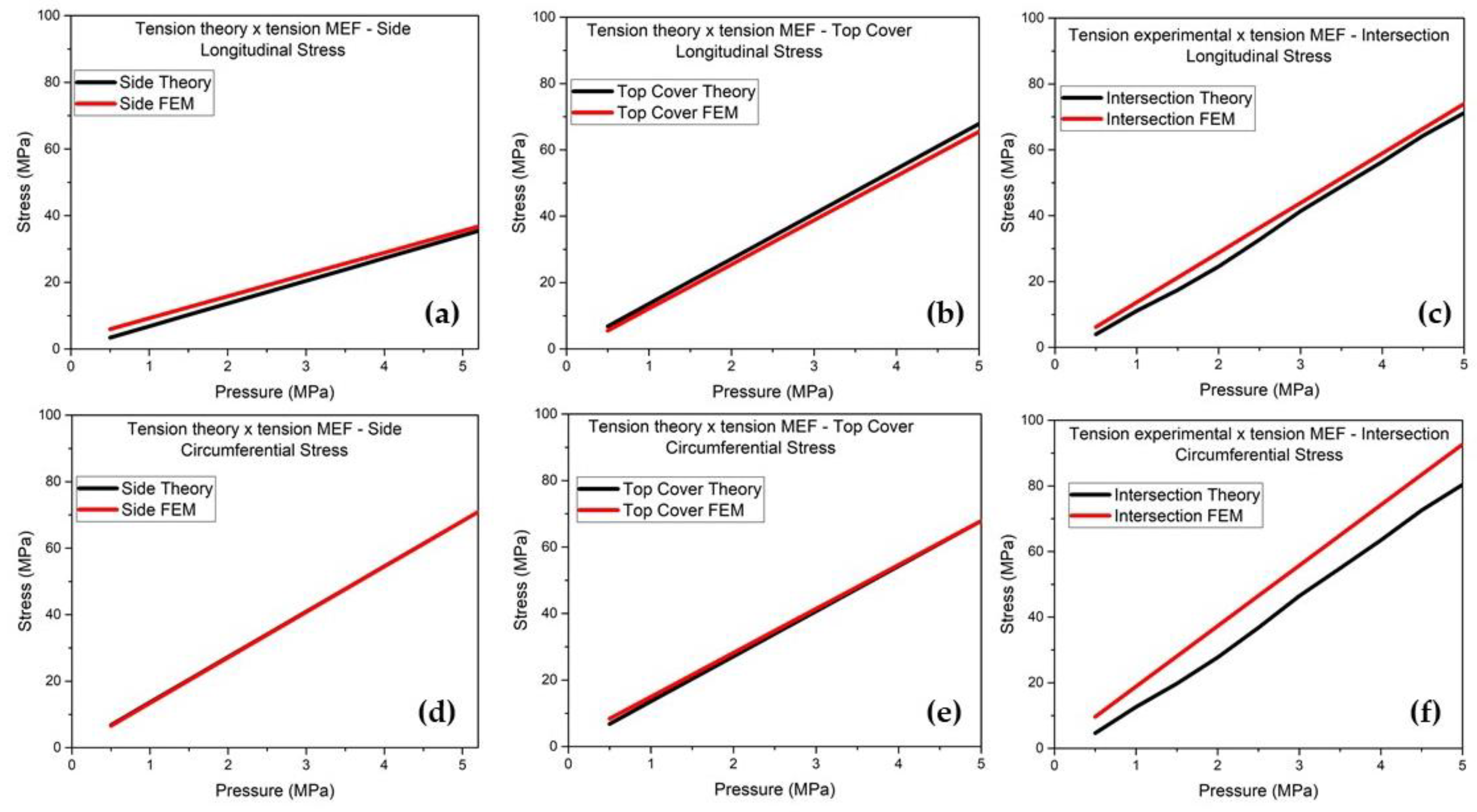
To improve understanding of the curves and verify how close the results were obtained, Figure 18 shows details of Figure 15, Figure 16 and Figure 17 for the six situations: Side (a) Longitudinal and (d) Circumferential, Top Cover (b) Longitudinal and (e) Circumferential and Intersection (c) Longitudinal and (f) Circumferential. This image clearly shows the proximity of the stress curves and also that for the circumferential stress at the point located on the side, the stresses obtained by the membrane theory and by the finite element method are exactly the same. It can also be observed that the point that obtained a greater difference was the one located at the intersection for the circumferential stress, and that this difference may be mainly due to the theory that cannot predict the bending stresses at points of discontinuity.
Figure 17.
Details of the stress curves – from 0 to 5 MPa comparing the theoretical curves and those obtained by the FEM. Evaluating the points: Side (a) Longitudinal and (d) Circumferential, Top Cover (b) Longitudinal and (e) Circumferential and Intersection (c) Longitudinal and (f) Circumferential.
5. Conclusions
Based on the stress results obtained through the three analyses, it was possible to observe that the values of the longitudinal and circumferential stresses obtained by the experimental analysis are lower than the values obtained by the analyses of the membrane theory, ASME code and the FEM at the two distant points of geometric discontinuity (side and top). However, for the point close to the geometric discontinuity (intersection of the top with the connection), the values of the longitudinal and circumferential stresses obtained by the experimental analysis are higher than the values obtained by the analyses of the membrane theory and ASME code, although lower than the FEM values, demonstrating in practice that in the regions close to the geometric discontinuity there are bending stresses that are not considered by the membrane theory and ASME code, but that are obtained by the FEM. It was also possible to observe that the region of intersection of the top with the connection obtained the highest stress value of the entire pressure vessel (disregarding the body of the connection), thus being the most critical region. The linearization of the stress obtained by the ANSYS software demonstrated that the bending stress has very low values when compared to the membrane stress along the thickness of the pressure vessel wall for the two specific points distant from geometric discontinuities, which is consistent with the membrane theory, in which the bending stress is neglected.
The numerical analysis, using the finite element method in the ANSYS software, proved to be a powerful and reliable tool in the analysis of stresses in pressure vessels, as it allows the analysis of stresses in critical regions, such as regions close to geometric discontinuities.
Author Contributions
Conceptualization, D.G., F. J. G. and M. S. M.; methodology, D.G., A. R. F. N., F. J. G. and M. S. M.; software, D. G. and E. S. G.; validation, D. G. and R. M. P.; formal analysis, D. G., A. R. F. N., E. S. G. F. J. G. S. F. M. A. and M. S. M.; investigation, D. G. and R. M. P.; resources, D. G. and M. S. M.; data curation, D. G., A. R. F. N., E. S. G. F. J. G. S. F. M. A..; writing—original draft preparation, D. G., A. R. F. N., E. S. G. F. J. G. S. F. M. A.; writing—review and editing, A. R. F. N., E. S. G. F. J. G. S. F. M. A.; visualization, S. F. M. A. and M. S. M.; supervision, S. F. M. A. and M. S. M.; project administration, F. J. G., S. F. M. A. and M. S. M.; funding acquisition, M.S.M. All authors have read and agreed to the published version of the manuscript.
Funding
Please add: This study was financed in part by the Coordenação de Aperfeiçoamento de Pessoal de Nível Superior-Brasil (CAPES)-Finance Code 001.
Acknowledgments
The authors would like to thank Universidade de Taubaté, UNESP and CAPES for their financial support.
Conflicts of Interest
The authors declare no conflicts of interest.
References
- Telles, P. C. S. Vasos de pressão, 2nd ed.; LTC Editora, Rio de Janeiro, Brazil, 2012.
- Krüger, R. L. Stress analysis in cylindrical pressure vessel nozzles: comparison between the WRC 297 bulletin method and the finite element method. Master's dissertation in Computational Modeling and Industrial Technology, Slavador – Brazil, 2014.
- Dubal, S.; Kadam, H. Pressure Vessel Accidents: Safety Approach. IRJET, 2017, v.30, n.1, p. 125-128.
- Kharat, A.; Kulkarni., V. V. Stress Concentration at openings in pressure vessels – A review. International Journal of Innovative Research in Science, Engineering and Technology, 2013, v.2, n.3, p.670-678.
- Dally, W. J.; Riley, F. W. Experimental Stress Analysis, 3rd ed.; McGrawl-Hill, Tokyo, Japan, 1978.
- Melo, E. M.; Albuquerque, P. J. R. Use of Electrical Resistance Strain Gauges for Instrumentation of Steel Piles. In Proceedings of 17 Brazilian Congress of Soil Mechanics and Geotechnical Engineering, Brazil, 03 May 2014.
- Niranjana, S. J.; Patel, S. V.; Dubey, A. K. Design and Analysis of Vertical Pressure Vessel using ASME Code and FEA Technique. IOP Conf. Series: Materials Science and Engineering 376, 2018.
- Gonçalves, C. P. Stress analysis using the finite element method in pressure vessel design: a case study in the sugarcane industry. Master’s thesis in Mechanical Project, Bauru – Brazil, 2016.
- Silva, A. B. Pressure vessel design according to ASME standard and finite element method. Master’s Thesis in Mechanical Project, Recife – Brazil, 2015.
- Krüger, R. L. Stress analysis in cylindrical pressure vessel nozzles: comparison between the WRC 297 bulletin method and the finite element method, Master’s Thesis in Computational Modeling and Industrial Technology, Salvador – Brazil, 2014.
- Grupta, S.R.; Vora, C. P. A review paper on pressure vessel design and analysis. International Research Journal of Engineering and Technology (IRJET). v.3, n.3, p. 295-300, 2014.
- Unnava, C. R.; Ramakrishna, C. H. Design and analysis of spherical shell with radial nozzle in pressure vessel. International Journal of Advanced Engineering Research and Studies. v.3, n.1, p. 52-54, 2013.
- Mendonça, D. P. Stress analysis using the finite element method of a pressure vessel designed according to ASME code. Master's thesis in Nuclear Technology, São Paulo – Brazil, 2021.
- Miranda, J. R. F. Analysis of stresses acting at intersections between nozzles and cylindrical pressure vessels with and without reinforcement plate under internal pressure. Master’s Thesis in Mechanical Project, Minas Gerais – Brazil, 2007.
- American Society of Mechanical Engineers. ASME Boiler and pressure vessel code: Rules for construction of pressure vessels, Section VIII, Division 2. New York, 2013.
- Figueiredo, C. D. R. Numerical methodology for the analysis of elastic stresses in the design by analysis of nuclear pressure vessels. Master's thesis in Projects, São Paulo – Brazil, 2011.
- Simulescu, I.; Mochio, T.; Shinozuka, M. Equivalent linearization method in nonlinear FEM. Journal of Engineering Mechanics, 1989, v. 115, n. 3, p. 475-492. [CrossRef]
- Wadkar, V. V.; Malgrave, S. S.; Patil, D. D.; Bhore, H. S.; Gavade, P. P. Design and analysis of pressure vessel using ANSYS. J. Mech. Eng. Technol, 2015, v. 3, n. 2, p. 1-13.
- Devatakonda, V. R. G. Finite element analysis (FEA) for stress evaluation of pressure vessel nozzles. International Journal of Core Engineering & Management, 2023, v. 7.
- Rigo, C. S. S. et al. Development of the Steering System for a Formula SAE Prototype. SAE Technical Paper, 2024.
- Gomes, L. O. et al. Brake Pedal Sizing and Preliminary Design of Balance Bar in the Brake of a SAE Formula Type Vehicle. SAE Technical Paper, 2024.
Figure 1.
Summary of the methodology adopted in this work for numerical, experimental and theoretical analysis of a pressure vessel.
Figure 1.
Summary of the methodology adopted in this work for numerical, experimental and theoretical analysis of a pressure vessel.
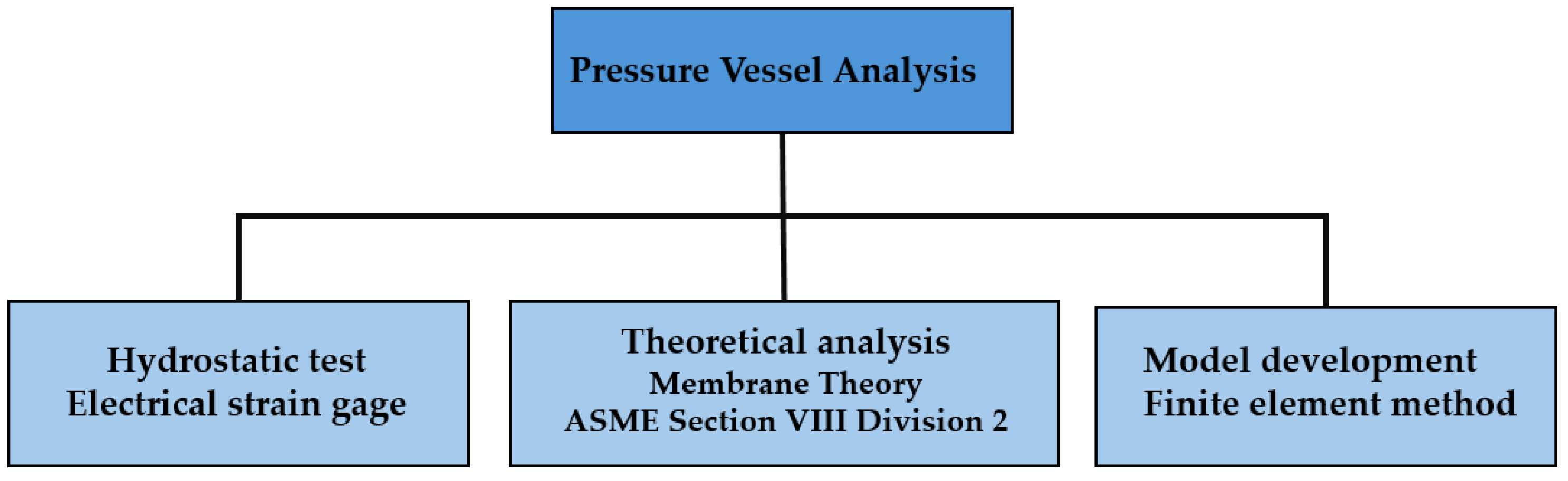
Figure 2.
Manufacturer's design.
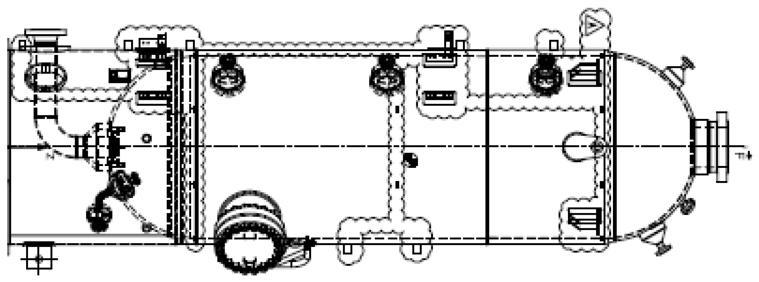
Figure 3.
(a) Pressure vessel positioned for hydrostatic testing; (b) Flange with pressure gauge; (c) General view of the pressure vessel with three specific points: top cover (yellow circle), intersection of the top cover with the connection (yellow square) and side (yellow triangle); (d) Positioning of the strain gauge close to the intersection, where the numbers noted on each rectangular rosette served to identify the deformations reported in the report issued by the signal conditioner.
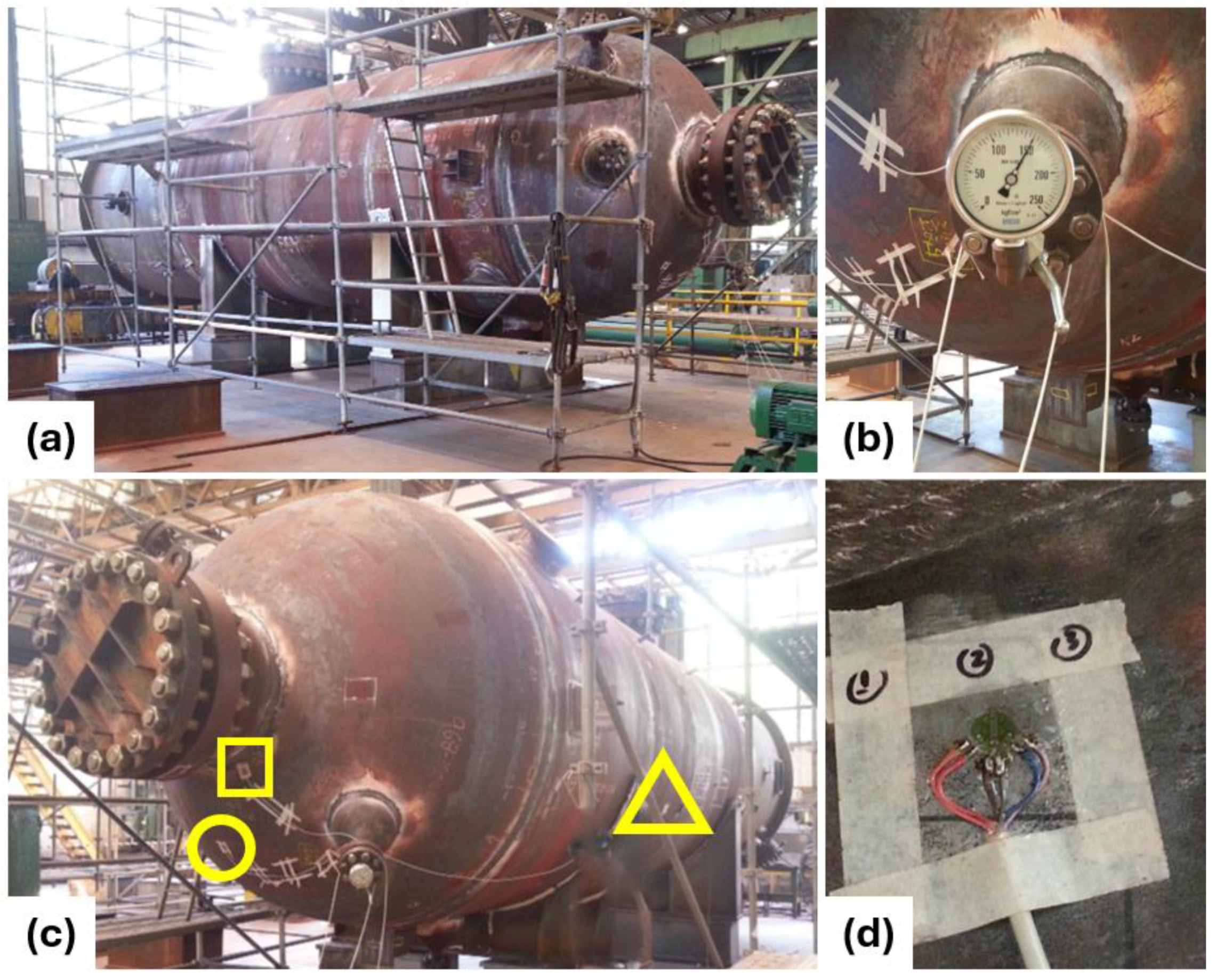
Figure 4.
(a) Overview of the complete pressure vessel model; (b) Overview of the simplified pressure vessel model.
Figure 4.
(a) Overview of the complete pressure vessel model; (b) Overview of the simplified pressure vessel model.

Figure 5.
Plans for section of the side and upper deck.
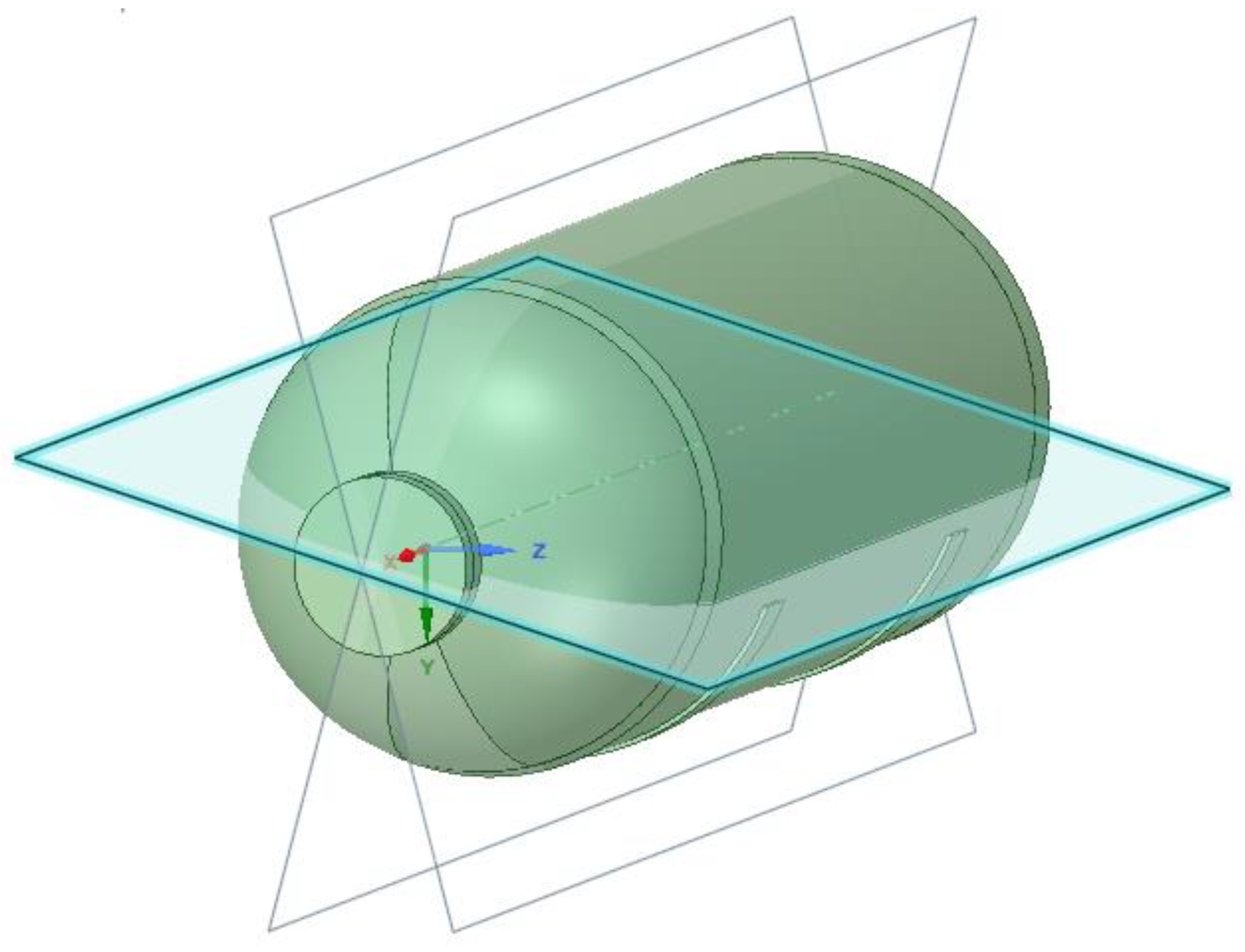
Figure 6.
Element quality for model mesh.
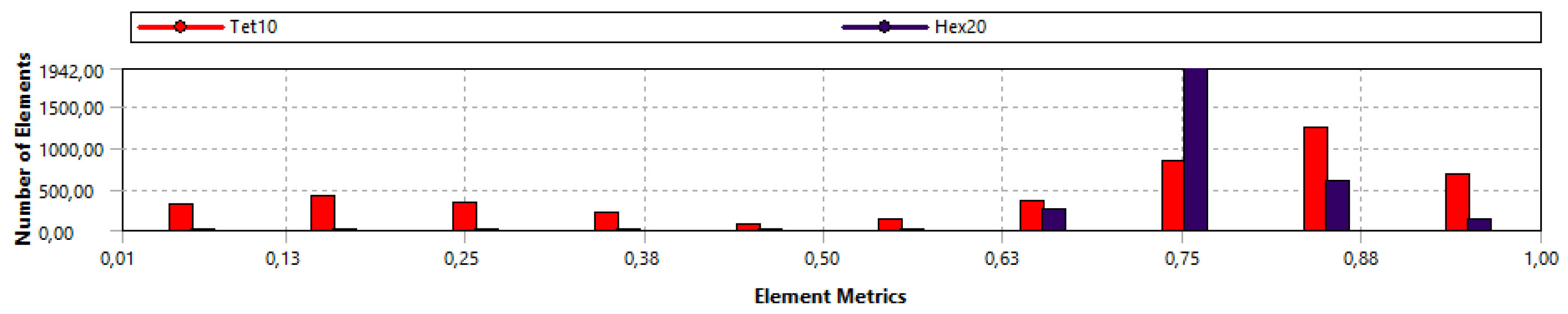
Figure 7.
(a) Longitudinal and (b) circumferential stresses calculated based on membrane theory.
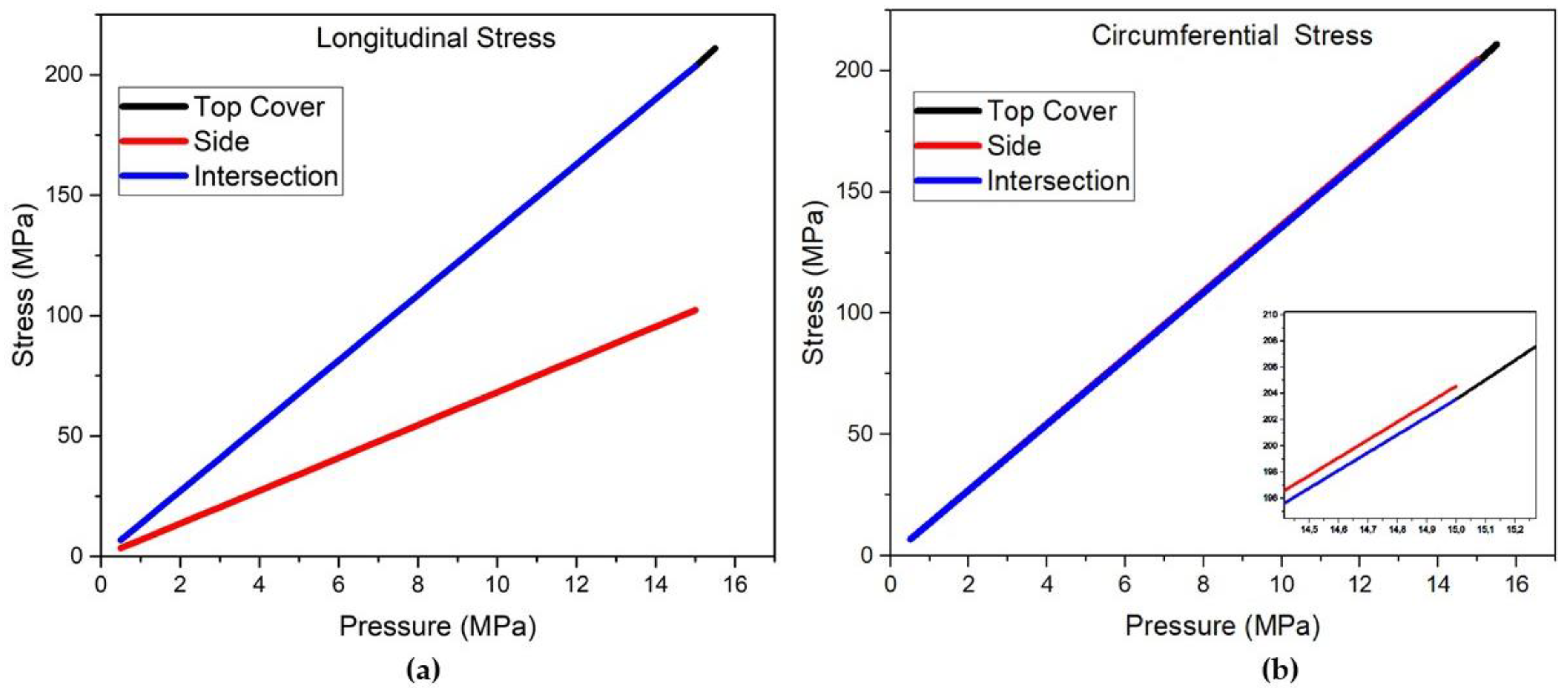
Figure 8.
(a) Longitudinal and (b) circumferential stresses calculated based on ASME code formulations.
Figure 8.
(a) Longitudinal and (b) circumferential stresses calculated based on ASME code formulations.
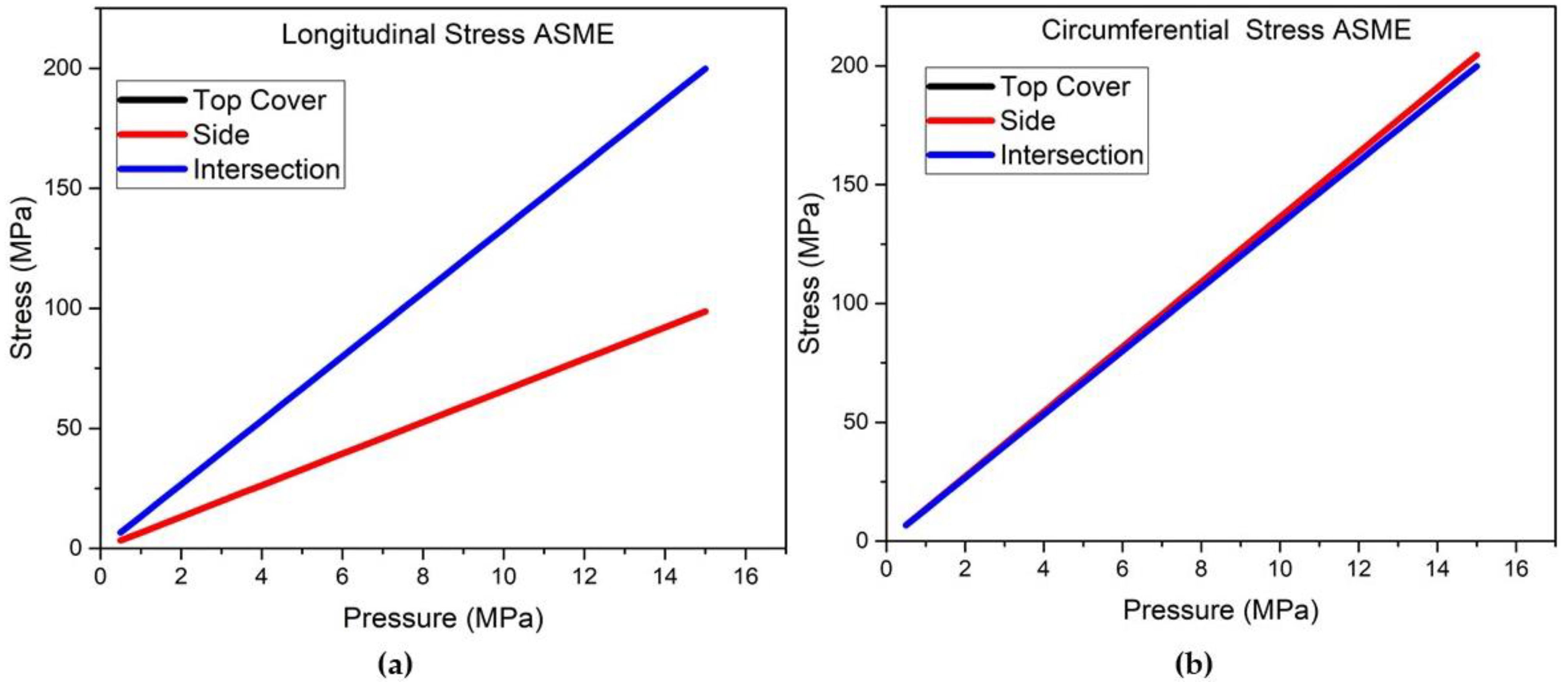
Figure 9.
(a) Longitudinal and (b) circumferential stresses calculated based on experimental data.
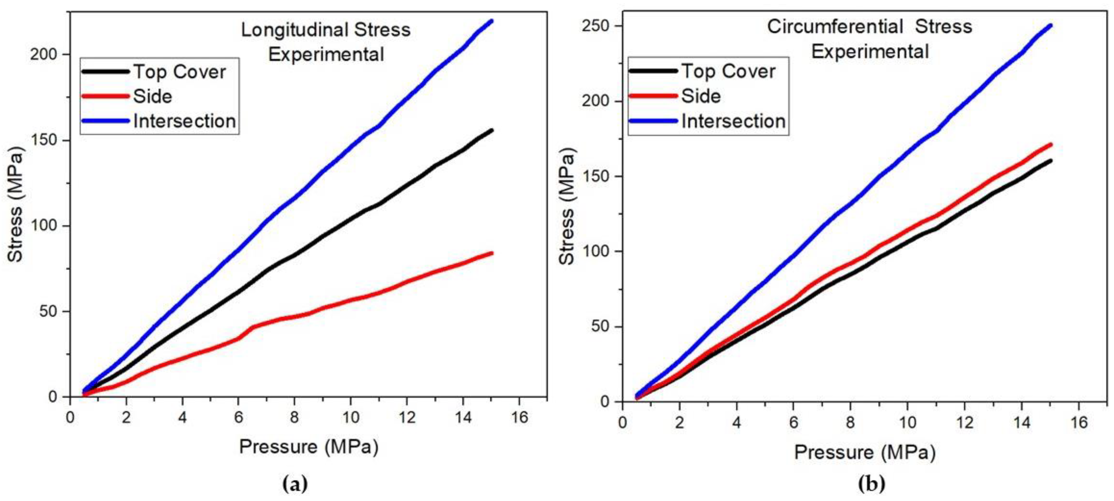
Figure 10.
(a) Longitudinal and (b) circumferential stresses calculated through modeling and simulation using ANSYS software.
Figure 10.
(a) Longitudinal and (b) circumferential stresses calculated through modeling and simulation using ANSYS software.
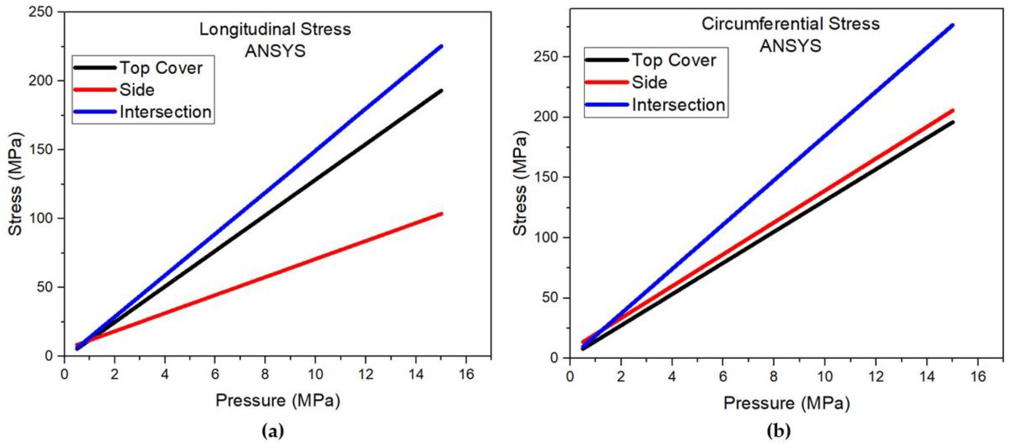
Figure 11.
(a) External view of the side (b) Mapping of circumferential stress on the outer surface of the side.
Figure 11.
(a) External view of the side (b) Mapping of circumferential stress on the outer surface of the side.
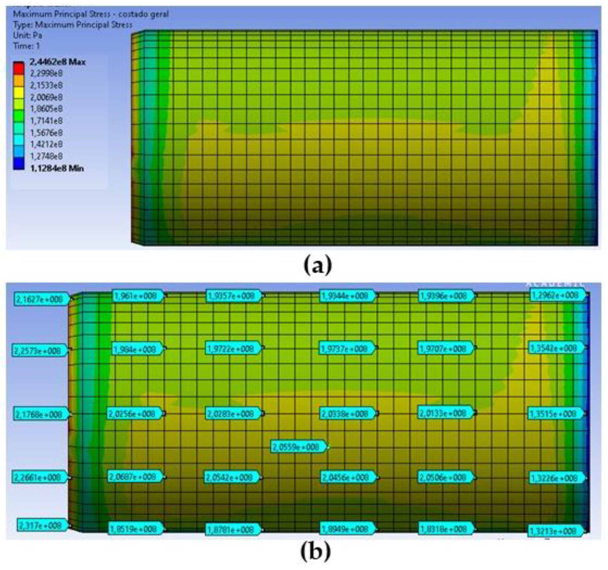
Figure 12.
(a) External view of top cover (b) Mapping of circumferential stress on the outer surface of the top cover.
Figure 12.
(a) External view of top cover (b) Mapping of circumferential stress on the outer surface of the top cover.
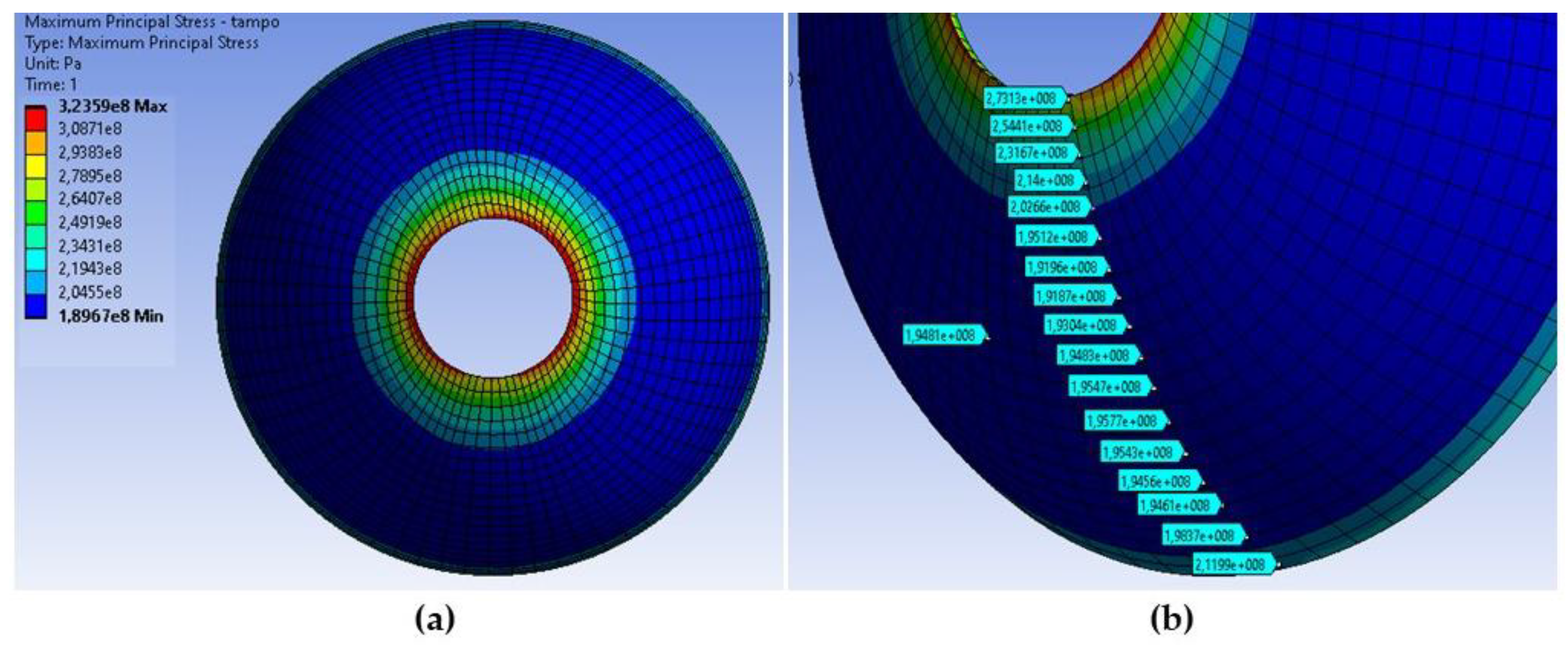
Figure 13.
(a) External view of pressure vessel (b) Detail of the region with the greatest circumferential stress of the pressure vessel.
Figure 13.
(a) External view of pressure vessel (b) Detail of the region with the greatest circumferential stress of the pressure vessel.
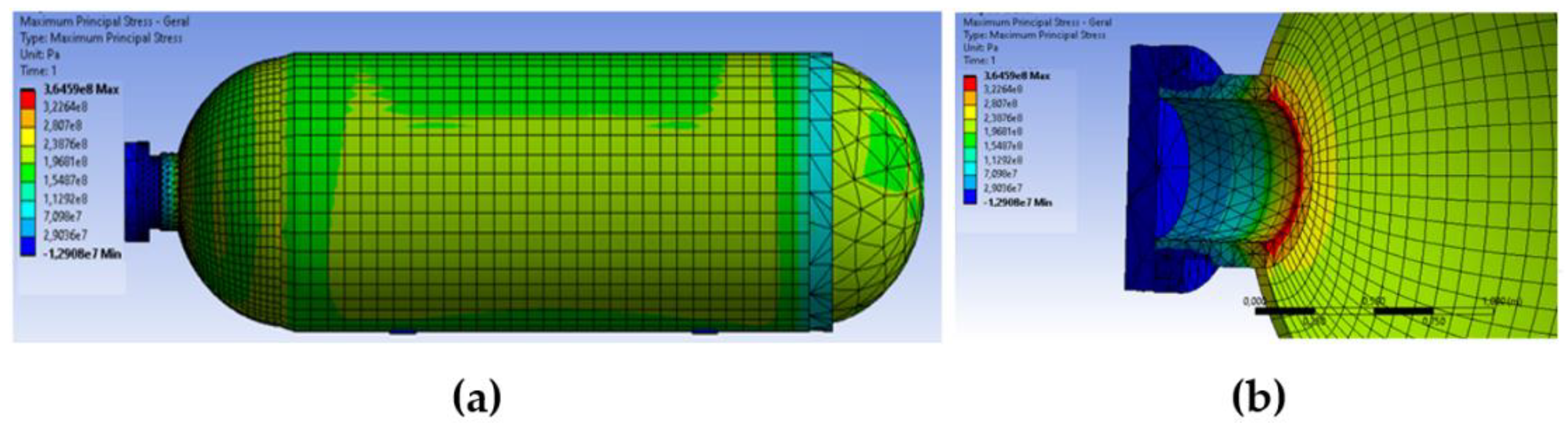
Figure 14.
Linearization of the circumferential stress at a specific point on the side.
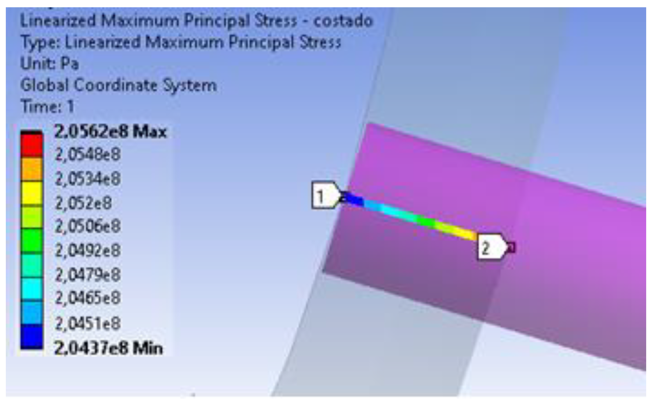
Figure 15.
Comparison of (a) longitudinal and (b) circumferential stress between theoretical stress and FEM - Side.
Figure 15.
Comparison of (a) longitudinal and (b) circumferential stress between theoretical stress and FEM - Side.
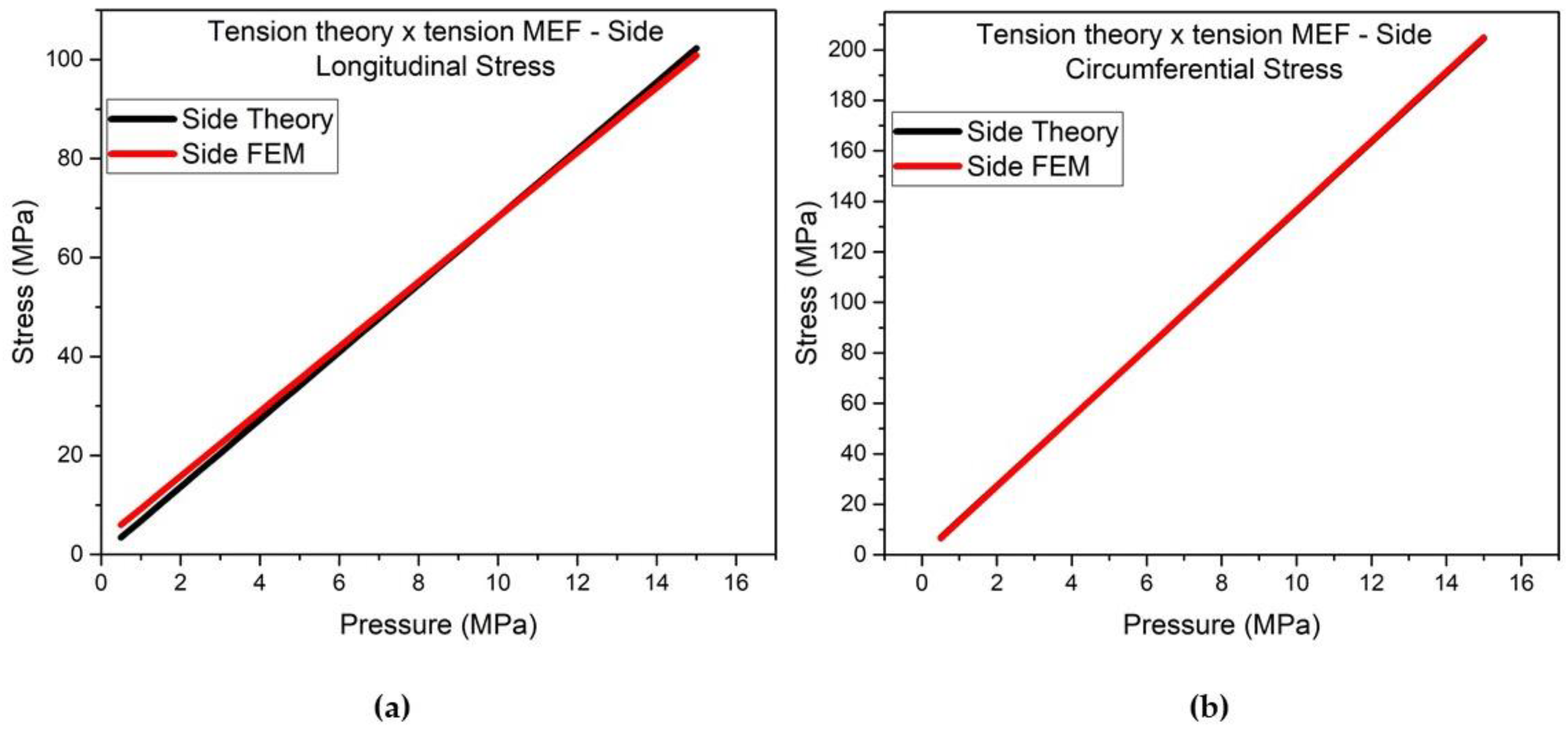
Figure 16.
Comparison of (a) longitudinal and (b) circumferential stress between theoretical stress and FEM – Top Cover.
Figure 16.
Comparison of (a) longitudinal and (b) circumferential stress between theoretical stress and FEM – Top Cover.
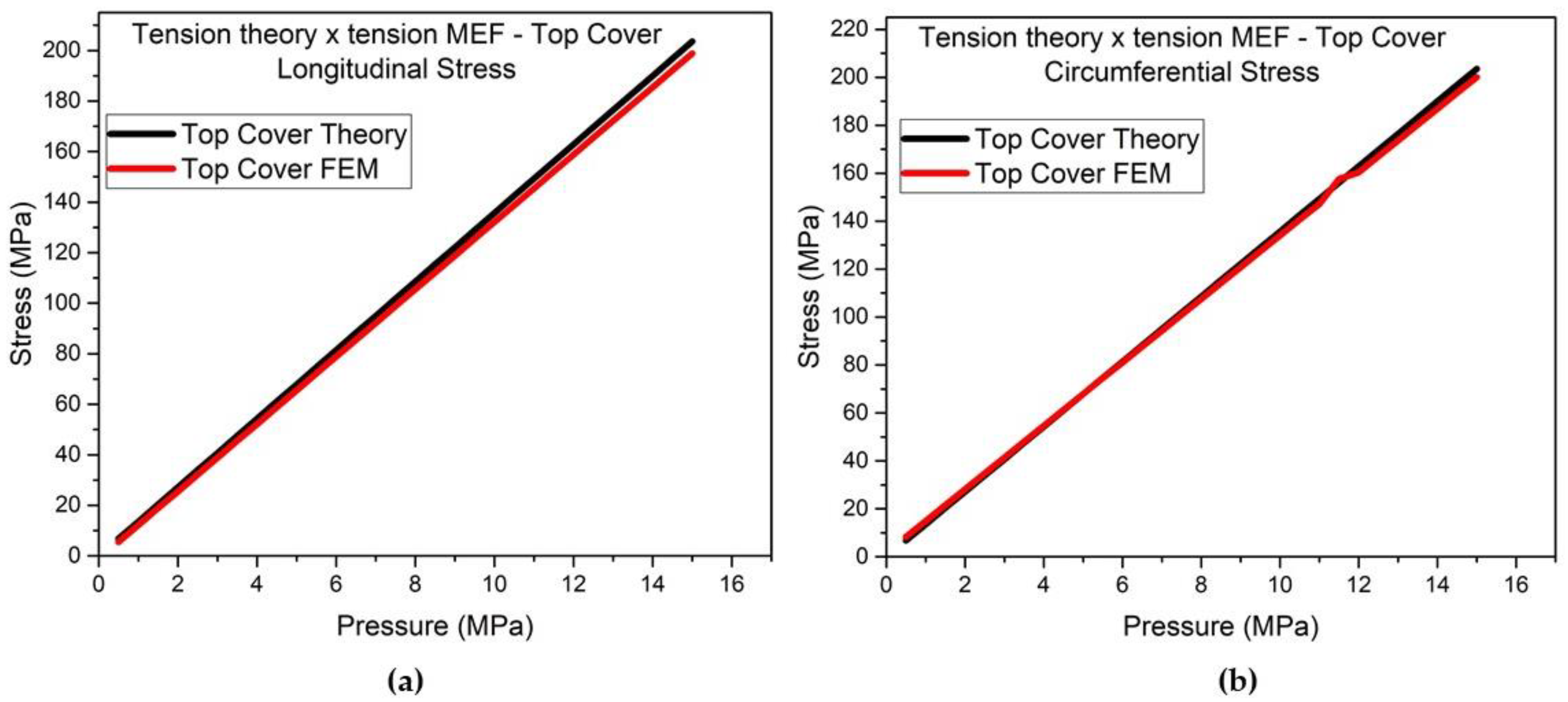
Figure 17.
Comparison of (a) longitudinal and (b) circumferential stress between experimental stress and FEM – Intersection.
Figure 17.
Comparison of (a) longitudinal and (b) circumferential stress between experimental stress and FEM – Intersection.
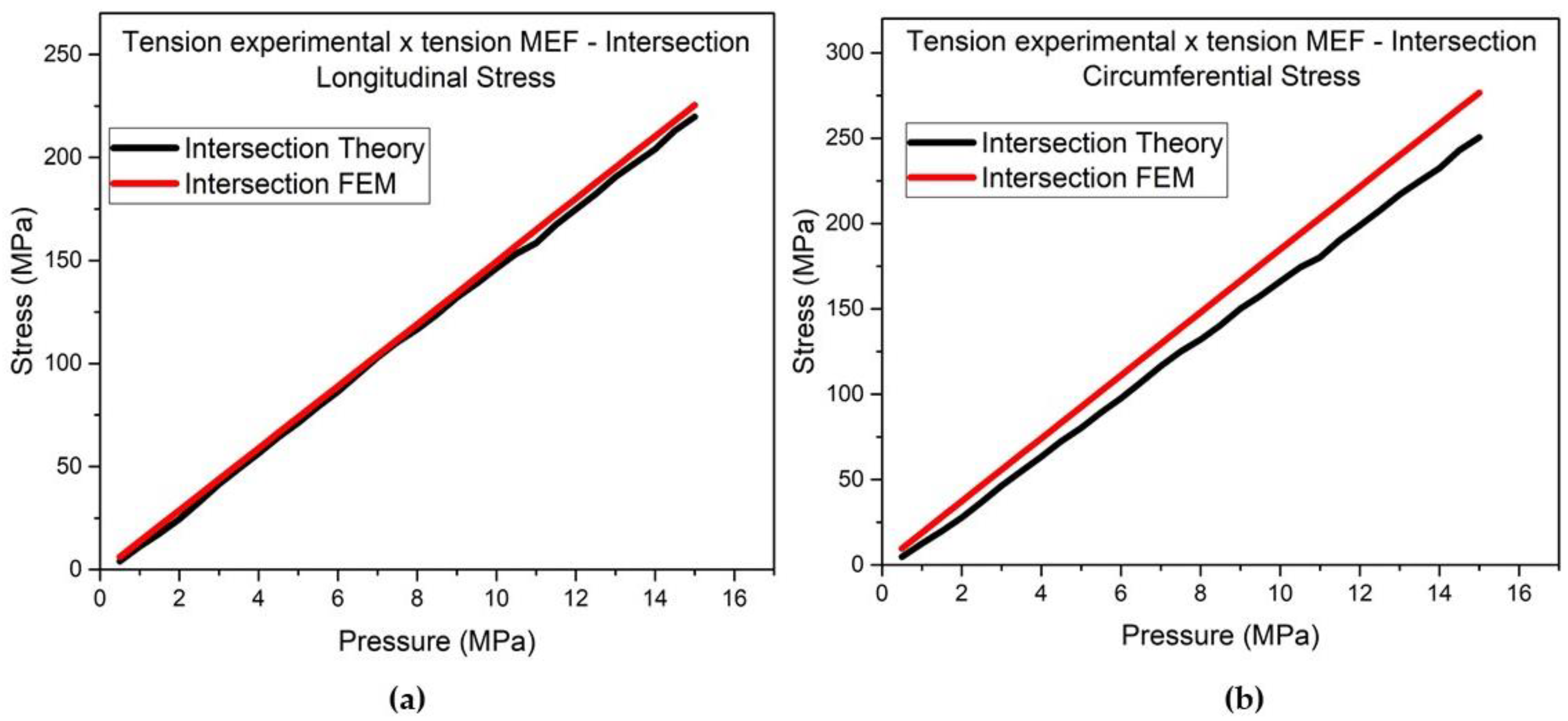
Table 1.
Basic pressure vessel information.
| Applied standards | ASME SECTION VIII DIV. 2 (2013) + NR 13 |
|---|---|
| Side and top material | SA 516 Gr 70 + CLAD 316 L |
| Yield strength - SA 516 Gr 70 | 262 MPa |
| Rupture strength - SA 516 Gr 70 | 482 MPa |
| Modulus of elasticity (E) - SA 516 Gr 70 | 200 GPa |
| Poisson's ratio - SA 516 Gr 70 | 0,30 |
| Side / top geometry | cilíndrica / semiesférica |
| Side thickness | 99 mm / 96 mm + 3 mm CLAD |
| Top thickness | inferior 50 mm / superior 47 mm + 3 mm |
| Operating pressure | 73,59 bar normal / 78,50 bar máxima |
| Operating temperature | 25 °C normal / 260 °C máxima |
| Design pressure | 92,02 bar |
| Design temperature | -46 °C mínima / 290 °C máxima |
| Side inside diameter | 2700 mm |
| Top inside diameter | 2714 mm |
| Welded joint efficiency Total Length |
1 10800 mm |
Table 2.
Deformations at a specific point on the top cover.
| Pressure (MPa) | εl (μ/μm) | ε45° (μ/μm) | εt (μ/μm) | Pressure (MPa) | εl (μ/μm) | ε45° (μ/μm) | εt (μ/μm) |
|---|---|---|---|---|---|---|---|
| 0.5 | 10.50 | 9.74 | 8.92 | 8.0 | 288.66 | 288.66 | 300.20 |
| 1.0 | 28.04 | 28.09 | 26.38 | 8.5 | 306.58 | 306.58 | 318.83 |
| 1.5 | 42.68 | 43.26 | 41.72 | 9.0 | 326.57 | 326.57 | 340.23 |
| 2.0 | 60.25 | 61.38 | 60.19 | 9.5 | 343.66 | 343.66 | 357.89 |
| 2.5 | 82.19 | 83.16 | 81.56 | 10.0 | 361.88 | 361.88 | 376.66 |
| 3.0 | 103.93 | 105.88 | 104.11 | 10.5 | 378.44 | 378.44 | 394.85 |
| 3.5 | 123.20 | 124.97 | 124.10 | 11.0 | 391.48 | 391.48 | 407.78 |
| 4.0 | 141.45 | 143.65 | 143.53 | 11.5 | 410.21 | 410.21 | 430.29 |
| 4.5 | 159.51 | 163.07 | 163.48 | 12.0 | 429.54 | 429.54 | 450.96 |
| 5.0 | 176.64 | 179.95 | 181.66 | 12.5 | 447.48 | 447.48 | 469.90 |
| 5.5 | 196.05 | 199.98 | 202.61 | 13.0 | 468.51 | 468.51 | 492.27 |
| 6.0 | 214.67 | 218.95 | 221.54 | 13.5 | 484.36 | 484.36 | 509.46 |
| 6.5 | 235.31 | 239.70 | 243.30 | 14.0 | 500.81 | 500.81 | 527.27 |
| 7.0 | 257.39 | 260.82 | 265.74 | 14.5 | 522.43 | 522.43 | 549.62 |
| 7.5 | 274.54 | 279.26 | 284.57 | 15.0 | 540.01 | 540.01 | 567.80 |
Table 3.
Deformations at a specific point on the side.
| Pressure (MPa) | εl (μ/μm) | ε45° (μ/μm) | εt (μ/μm) | Pressure (MPa) | εl (μ/μm) | ε45° (μ/μm) | εt (μ/μm) |
|---|---|---|---|---|---|---|---|
| 0.5 | 02.82 | 07.17 | 13.24 | 8.0 | 100.25 | 212.21 | 387.86 |
| 1.0 | 08.21 | 20.79 | 37.89 | 8.5 | 101.65 | 223.47 | 410.38 |
| 1.5 | 09.98 | 30.37 | 57.92 | 9.0 | 108.51 | 238.09 | 437.84 |
| 2.0 | 16.93 | 44.06 | 82.55 | 9.5 | 111.67 | 250.58 | 459.66 |
| 2.5 | 27.81 | 61.80 | 111.50 | 10.0 | 116.21 | 263.22 | 483.92 |
| 3.0 | 36.48 | 78.72 | 140.37 | 10.5 | 116.92 | 275.74 | 507.63 |
| 3.5 | 42.30 | 93.37 | 165.46 | 11.0 | 122.81 | 285.60 | 524.69 |
| 4.0 | 47.21 | 106.71 | 190.13 | 11.5 | 130.16 | 293.35 | 548.64 |
| 4.5 | 53.21 | 118.10 | 214.36 | 12.0 | 138.12 | 310.58 | 576.26 |
| 5.0 | 57.74 | 130.58 | 237.49 | 12.5 | 143.18 | 324.58 | 601.96 |
| 5.5 | 63.41 | 145.51 | 263.73 | 13.0 | 148.63 | 339.51 | 269.61 |
| 6.0 | 70.86 | 160.12 | 289.03 | 13.5 | 153.25 | 351.83 | 651.45 |
| 6.5 | 93.68 | 176.34 | 317.34 | 14.0 | 157.99 | 363.80 | 673.41 |
| 7.0 | 96.41 | 191.71 | 345.04 | 14.5 | 164.05 | 379.95 | 702.40 |
| 7.5 | 99.74 | 203.70 | 368.37 | 15.0 | 169.21 | 392.41 | 725.13 |
Table 4.
Deformations at the specific point of intersection.
| Pressure (MPa) | εl (μ/μm) | ε45° (μ/μm) | εt (μ/μm) | Pressure (MPa) | εl (μ/μm) | ε45° (μ/μm) | εt (μ/μm) |
|---|---|---|---|---|---|---|---|
| 0.5 | 16.42 | 13.31 | 13.90 | 8.0 | 468.46 | 397.15 | 401.77 |
| 1.0 | 44.46 | 37.70 | 38.68 | 8.5 | 497.95 | 421.78 | 426.35 |
| 1.5 | 69.56 | 59.06 | 60.54 | 9.0 | 532.93 | 449.99 | 454.64 |
| 2.0 | 98.44 | 83.85 | 84.63 | 9.5 | 559.13 | 472.96 | 478.30 |
| 2.5 | 130.47 | 111.78 | 111.78 | 10.0 | 589.99 | 498.80 | 503.68 |
| 3.0 | 164.51 | 141.24 | 141.24 | 10.5 | 618.59 | 522.36 | 527.77 |
| 3.5 | 194.13 | 166.69 | 166.69 | 11.0 | 639.99 | 540.12 | 545.69 |
| 4.0 | 224.41 | 192.17 | 192.17 | 11.5 | 676.57 | 570.46 | 575.71 |
| 4.5 | 256.68 | 218.77 | 222.34 | 12.0 | 706.76 | 595.90 | 601.29 |
| 5.0 | 284.32 | 242.31 | 246.09 | 12.5 | 737.18 | 621.10 | 626.83 |
| 5.5 | 315.61 | 269.01 | 273.35 | 13.0 | 771.68 | 650.40 | 655.28 |
| 6.0 | 345.61 | 294.16 | 298.13 | 13.5 | 799.40 | 673.33 | 678.30 |
| 6.5 | 378.79 | 322.02 | 326.51 | 14.0 | 826.61 | 696.50 | 700.87 |
| 7.0 | 412.80 | 351.00 | 355.62 | 14.5 | 863.60 | 726.80 | 731.85 |
| 7.5 | 443.11 | 376.41 | 380.58 | 15.0 | 891.89 | 750.65 | 754.45 |
Table 5.
Variation of theoretical, ASME, experimental and FEM analyses in the side, top cover and intersection to 3 MPa.
Table 5.
Variation of theoretical, ASME, experimental and FEM analyses in the side, top cover and intersection to 3 MPa.
| Point at 3 MPa | σMembrane (MPa) | σASME (MPa) | σExperimental (MPa) σFEM(MPa) | |||||
|---|---|---|---|---|---|---|---|---|
| Long. | Circumf. | Long. | Circumf | Long. | Circumf. | Long. | Circumf. | |
| Side | 20.45 | 40.91 | 19.73 | 40.91 | 17.13 | 33.39 | 24.85 | 46.72 |
| Top Cover | 40.71 | 40.71 | 39.97 | 39.97 | 29.43 | 30.01 | 37.85 | 40.38 |
| Intersection | 40.71 | 40.71 | 39.97 | 39.97 | 41.38 | 46.45 | 43.85 | 55.74 |
Disclaimer/Publisher’s Note: The statements, opinions and data contained in all publications are solely those of the individual author(s) and contributor(s) and not of MDPI and/or the editor(s). MDPI and/or the editor(s) disclaim responsibility for any injury to people or property resulting from any ideas, methods, instructions or products referred to in the content. |
© 2025 by the authors. Licensee MDPI, Basel, Switzerland. This article is an open access article distributed under the terms and conditions of the Creative Commons Attribution (CC BY) license (http://creativecommons.org/licenses/by/4.0/).
Copyright: This open access article is published under a Creative Commons CC BY 4.0 license, which permit the free download, distribution, and reuse, provided that the author and preprint are cited in any reuse.


