
Submitted:
19 January 2026
Posted:
20 January 2026
You are already at the latest version
Abstract
This paper presents a comparative analysis of natural gas and electric power prices using visibility graph methodology, a technique from complex network theory that transforms temporal sequences into network representations. We analyze 1,826 daily observations from the Italian energy market (2019-2023), implementing a three-stage preprocessing pipeline (logarithmic transformation, LOESS detrending, and first differencing) before constructing visibility graphs. Our topological analysis reveals striking differences: gas exhibits substantially higher connectivity (6,202 versus 5,354 edges), heavier-tailed degree distributions (maximum degree 117 versus 54), and dramatically longer-range connections (average temporal distance 26.4 versus 11.0 days). Paradoxically, despite power displaying twice the raw volatility, gas generates more structured long-range correlations due to storage-enabled intertemporal linkages. Both series exhibit small-world properties with high clustering (≈0.76), short path lengths (4.59 and 5.36), and positive assortativity (≈0.17). Correlation analysis reveals moderate contemporaneous return correlation (Pearson r = 0.456) with substantial time variation (range 0.173– 0.696), no lead-lag relationships, and partial synchronization of topological properties. Node-level degree and clustering show positive correlations between markets, while closeness centrality exhibits strong negative correlation (r = −0.719), indicating fundamentally different global network organization. Structural similarity (Jaccard coefficient 0.404) confirms 40% shared visibility connections with 60% commodity-specific structure. These findings demonstrate that physical storability fundamentally shapes temporal correlation structure, with direct implications for risk management, forecasting model selection, and portfolio construction in energy markets.
Keywords:
financial time series
; complex networks
; visibility graphs
; time series analysis
; natural gas prices
; electricity prices
; network topology
1. Introduction
1.1. The Challenge of Financial Time Series Analysis
Energy markets represent one of the most economically significant sectors globally, with natural gas and electric power playing critical roles in industrial production, transportation, and modern infrastructure. Understanding price dynamics is essential for traders, utilities, industrial consumers, portfolio managers, and regulators navigating volatile energy markets.
Financial time series analysis has been a cornerstone of quantitative research for over half a century [1]. Researchers have developed extensive toolkits including autocorrelation analysis, ARIMA models, GARCH frameworks, and machine learning approaches [2,3]. However, traditional methods face fundamental limitations when confronted with real-world financial data complexity. Three problematic characteristics challenge traditional frameworks: non-stationarity (time-varying means, variances, and correlation structures), nonlinearity (asymmetric responses, threshold effects, feedback loops), and extreme events (fat-tailed distributions that expose inadequately-captured tail risks) [4].
These challenges are particularly acute in electricity markets, where physical constraints create price dynamics fundamentally different from purely financial markets. Traditional ARIMA models fail to adequately represent sudden jumps characteristic of electricity prices, while GARCH models struggle with extreme asymmetry. In recent years, researchers have increasingly turned to complex network theory and graph-theoretical methods as alternative frameworks [5,6,7]. The fundamental insight is that temporal sequences can be transformed into network representations, offering nonlinear correlation capture, robustness to non-stationarity, intuitive visualizations, and connection to complex systems science.
1.2. Visibility Graphs: Philosophy and Geometric Intuition
The visibility graph (VG) algorithm [8] stands out for its conceptual elegance and computational simplicity. Rather than imposing arbitrary transformations or parametric assumptions, the method asks a natural geometric question: can two points in a time series “see” each other?
Consider a time series as a landscape profile where time progresses horizontally and values represent vertical elevations. Two data points and with are mutually visible if all intermediate points for satisfy:
The right-hand side represents the straight line from point i to point j at time . This natural geometric mapping exhibits remarkable mathematical properties [8,9]: affine invariance, deterministic structure preservation, and deep connections between degree distributions and statistical properties of the underlying time series.
Previous empirical and theoretical studies have demonstrated the power and versatility of visibility graph analysis across diverse application domains, establishing it as a mature methodological framework with growing adoption across disciplines. Lacasa and colleagues showed that visibility graphs can estimate the Hurst exponent of fractional Brownian motion, providing a novel method for detecting long-range correlations and distinguishing between persistent, anti-persistent, and uncorrelated processes [10]. This connection between degree distribution properties and temporal correlation structure has been rigorously established through both analytical derivations and numerical simulations [9,11].
In financial markets, visibility graph analysis has characterized stock price dynamics [12], cryptocurrency exchanges [13], bubble formation [14], and increasingly energy commodity prices [14,15]. The method has proven particularly valuable in finance because it makes no parametric assumptions about return distributions, handles non-stationarity naturally [16], and can detect regime changes through evolving network topology [17].
1.3. Physical and Economic Foundations of Energy Markets
Energy markets exhibit distinctive characteristics distinguishing them from traditional financial markets [18,19,20], arising from physical commodity nature, engineering constraints, and regulatory frameworks.
The most fundamental and consequential distinction is the issue of storability. Natural gas, being a physical commodity that can be compressed and stored in underground caverns, depleted reservoirs, or liquefied natural gas (LNG) facilities, possesses a degree of intertemporal substitutability: gas purchased today can be stored and consumed tomorrow, next week, or next winter. This storage capability creates arbitrage linkages across time, connecting current prices to expected future prices through storage economics characterized by storage costs, injection and withdrawal capacities, and opportunity costs of capital.
The ability to store gas has profound implications for price dynamics: it dampens short-term price volatility by allowing supply-demand imbalances to be absorbed through inventory adjustments; it creates seasonal price patterns reflecting winter heating demand and summer injection seasons; and it establishes price relationships across geographically separated markets through the potential for transportation and storage. Moreover, storage creates recurring price thresholds and reference levels as inventories approach capacity constraints or depletion limits.
In stark contrast, electricity suffers from the constraint of essential non-storability at economically relevant scales. While battery storage technology is advancing rapidly and pumped hydro storage exists in some locations, the overwhelming majority of electricity must be generated at the precise instant it is consumed. This physical constraint has dramatic consequences for price formation.
Supply and demand must be balanced continuously in real-time to maintain grid frequency and voltage stability; any instantaneous mismatch creates immediate and potentially catastrophic system stress requiring emergency interventions. Consequently, when demand unexpectedly surges (for example, during extreme weather events) or generation capacity suddenly fails (due to plant outages or renewable resource unavailability), prices can spike to values hundreds or even thousands of times higher than typical levels within minutes, only to crash back down just as quickly once balance is restored. These price spikes reflect not just scarcity rents but also the immense value that consumers place on avoiding blackouts and the high marginal costs of emergency peaking generation units that operate only during supply crises.
Second, electricity requires instantaneous supply-demand balance, creating characteristic patterns: frequent small fluctuations as the system adjusts, punctuated by occasional extreme spikes when approaching operational limits. Third, both markets exhibit strong weather dependence through different mechanisms and time scales. Gas demand peaks with winter heating, while electricity exhibits both winter and summer peaks. Increasing renewable penetration adds supply-side weather sensitivity [21].
Fourth, markets are interconnected through pervasive gas-fired electricity generation. Shocks propagate between markets: gas price spikes transmit to electricity as generation becomes expensive, while high electricity prices incentivize increased gas-fired generation. However, this relationship is asymmetric and nonlinear.
Understanding these structural differences is crucial for diverse market participants in risk management, contracting decisions, regulatory market design, and operational planning.
1.4. Research Objectives and Contributions
This paper pursues four interconnected research objectives that together constitute a comprehensive investigation into the comparative structure of natural gas and electric power price time series.
First, we aim to develop and apply a systematic, theoretically motivated preprocessing pipeline that transforms raw price data into a form suitable for visibility graph analysis while preserving economically relevant dynamical features. This pipeline consists of three sequential stages: logarithmic transformation to stabilize variance and convert multiplicative price dynamics into additive form (consistent with standard financial modeling where returns are the fundamental objects); LOESS nonparametric detrending to remove long-term non-stationary trends attributable to inflation, technological change, or structural shifts without imposing parametric functional forms; and first differencing to extract short-term incremental dynamics representing day-to-day price changes. Each preprocessing step serves a specific purpose, and we carefully document and justify these methodological choices, discuss their implications, and examine their effects on resulting time series characteristics.
Second, we aim to construct visibility graphs from the preprocessed gas and power price data, implementing the geometric visibility criterion rigorously. This involves applying the visibility algorithm to approximately 1,800 data points for each commodity, checking visibility conditions for potentially millions of point pairs, and generating undirected graphs that encode the temporal correlation structure of price fluctuations in network form. The visibility graph construction is the crucial transformation that allows us to move from the temporal domain to the network domain where topological properties can be analyzed using the rich toolkit of graph theory and network science.
Third, we aim to comprehensively characterize and compare topological properties of the resulting visibility graph networks using a battery of well-established network metrics. Specifically, we compute and analyze: basic connectivity measures including node and edge counts, network density, and degree statistics; degree distribution characteristics including mean, maximum, and distributional shape parameters; clustering coefficients quantifying the tendency of nodes to form tightly interconnected communities; path length metrics including average shortest path length and network diameter characterizing global connectivity; assortativity coefficients measuring whether similar-degree nodes preferentially connect; and temporal distance distributions for edges revealing whether connections are predominantly local (short-range) or global (long-range) in the time dimension. By systematically comparing these metrics between gas and power visibility graphs, we can identify structural differences reflecting underlying differences in market dynamics.
Fourth, and most importantly, we aim to interpret the observed differences in visibility graph structure in terms of underlying physical, economic, and market-structural factors driving gas and power price dynamics. This interpretive step is crucial for moving beyond statistical description to genuine understanding with actionable implications. We draw connections between network topology and market phenomena: relating heavy-tailed degree distributions to extreme price events; connecting long-range visibility to persistent memory effects and storage economics; linking clustering patterns to volatility clustering and regime persistence; and associating topological differences with fundamental physical distinctions like storability.
Fifth, we aim to systematically investigate the correlation structure between gas and power time series, complementing the individual visibility graph analyses with a comprehensive examination of their interdependencies. This includes computing multiple correlation measures (Pearson, Spearman, and Kendall coefficients) to assess linear and non-parametric associations between log-returns, performing cross-correlation analysis to detect potential lead-lag relationships and temporal precedence patterns, conducting rolling correlation analysis using sliding windows to track the time-varying nature of market coupling and identify regime changes, examining correlations between node-level topological properties (degree, clustering coefficient, betweenness and closeness centrality) of the two visibility graphs to understand whether extreme events and structural positions synchronize across markets, and measuring structural similarity through edge overlap (Jaccard similarity) to quantify the proportion of shared versus commodity-specific visibility connections. This correlation analysis is essential for understanding how these two energy commodities interact in practice, with direct implications for portfolio diversification, cross-commodity hedging strategies, and risk management. The moderate return correlations combined with distinct visibility graph topologies suggest that gas and power share some common dynamical patterns driven by shared market factors (weather shocks, economic conditions, fuel switching dynamics) while maintaining substantial independent structure reflecting their unique physical and economic characteristics.
The principal contribution of this work lies in providing the first systematic comparative visibility graph analysis of natural gas and electric power prices, revealing a striking and counterintuitive empirical finding: despite the conventional wisdom that electricity markets exhibit more extreme volatility than gas markets (a belief supported by simple volatility statistics), gas prices actually exhibit more structured extreme events and longer-range temporal dependencies as measured by visibility graph topology. This apparent paradox - higher raw volatility in power but more persistent visibility structure in gas - can be resolved through careful consideration of the physical and economic mechanisms discussed earlier, particularly the role of storage in creating intertemporal price linkages.
Our findings have direct practical implications for market participants: they suggest that gas price modeling requires methods capable of capturing long memory and extreme value persistence (perhaps ARFIMA models, regime-switching approaches, or recurrent neural networks with long-term dependencies), while power price modeling may be better served by approaches emphasizing short-term volatility dynamics and mean reversion (such as jump-diffusion processes or threshold GARCH models). Furthermore, our methodological framework is general and portable: the preprocessing and visibility graph analysis pipeline we develop can be readily applied to other financial time series, providing a template for future comparative studies across different commodities, markets, or time periods.
1.5. Organization of the Paper
The remainder of this paper is organized as follows. Section 2 presents the methodology, including detailed description of the dataset, the three-stage preprocessing pipeline (logarithmic transformation, LOESS detrending, and first differencing), the visibility graph construction algorithm, and the network metrics employed for topological characterization. Section 3 reports the empirical results, documenting preprocessing effects, comparing topological properties of gas and power visibility graphs (connectivity, degree distributions, clustering coefficients, path lengths, assortativity), and analyzing temporal distance distributions that reveal the fundamental differences in long-range correlation structure. Section 4 presents a comprehensive correlation analysis between gas and power time series, examining return correlations, cross-correlation functions, rolling correlations, correlations between visibility graph metrics, and structural similarity measures. Section 5 provides an in-depth discussion interpreting the observed topological differences in terms of physical and economic factors (storability, mean-reversion dynamics), identifying universal features shared across both commodities, deriving practical implications for risk management, forecasting, and portfolio construction, and addressing methodological considerations, limitations, and directions for future research. Section 6 concludes by synthesizing the principal findings and articulating the broader methodological and scientific impact of visibility graph analysis for understanding complex financial dynamics.
2. Methodology
2.1. Data Description and Characteristics
The empirical analysis is conducted on the Italian energy market, specifically using time series of natural gas and electricity prices provided by GME (Gestore dei Mercati Energetici SpA), the operator of Italian wholesale energy markets. Our dataset consists of daily frequency time series spanning from January 1, 2019, to December 31, 2023, yielding 1,826 observations for each commodity. This period is notable for its unique and turbulent conditions, including the impacts of the COVID-19 pandemic emergency beginning in early 2020, the subsequent onset of economic recovery in 2021-2022, and the extraordinary market turbulence caused by the Ukraine war beginning in February 2022. These factors make it an excellent testing ground for methodology robustness, as the data include both relatively normal market conditions and extreme stress episodes.
These datasets provide sufficient statistical power to characterize medium-term dynamics spanning approximately five years of trading activity. Most importantly, they cover an identical time period for both commodities, enabling direct comparative analysis while controlling for common external factors such as macroeconomic conditions, weather patterns, and regulatory environments that affect both markets simultaneously.
The first time series, Gas prices, consists of 1,826 consecutive daily observations of natural gas spot prices in the Italian market. Natural gas prices are influenced by a complex interplay of supply factors (domestic production levels, LNG and pipeline import availability, international market dynamics, infrastructure capacity constraints), demand factors (residential and commercial heating requirements, industrial consumption, power generation demand from gas-fired plants), storage dynamics (inventory levels, seasonal storage cycles, injection and withdrawal constraints, storage capacity utilization), and market structure considerations (number and behavior of market participants, liquidity, contract specifications, trading mechanisms). The raw gas price data, before any preprocessing, exhibit typical features of commodity price series including a general upward trend over portions of the sample period (potentially reflecting inflation, resource depletion pressures, or increasing demand), substantial volatility with day-to-day fluctuations of several percentage points being common, and occasional extreme spikes or drops corresponding to supply disruptions, demand shocks, or speculative dynamics.
The second time series, Power prices (or electricity prices), similarly consists of 1,826 consecutive daily observations representing electric power spot market prices over the same time period as the gas data. These prices reflect the marginal cost of generating electricity to meet demand at any given time, determined through organized wholesale market mechanisms such as day-ahead auctions or real-time balancing markets. As discussed in the introduction, electricity prices exhibit unique characteristics stemming from non-storability: they can display extreme volatility with spikes reaching values ten or even a hundred times normal levels during supply scarcity events (such as heat waves causing high air conditioning demand, cold snaps driving heating loads, or generator outages reducing available supply), followed by rapid returns to more typical levels once supply-demand balance is restored. The power price data in our sample reflect these dynamics, showing both the typical variations associated with daily and weekly demand cycles and the occasional extreme events that characterize electricity markets during stressed conditions.
A crucial methodological point is that both time series span an identical time period and represent daily frequency observations. This temporal alignment is essential for our comparative analysis: it ensures that both series experience the same macroeconomic environment, similar weather patterns (since gas and power markets often operate in the same geographic regions and respond to common weather-driven demand signals), common regulatory regimes, and synchronized market events such as the pandemic lockdowns or the energy crisis following the Ukraine invasion. Any differences we observe in their visibility graph structure can therefore be attributed to intrinsic differences in the price formation processes rather than to differences in external conditions or sample composition. The daily frequency, while not capturing the high-frequency intraday dynamics that can be important in electricity markets (where prices may vary hour by hour or even minute by minute), is appropriate for our focus on medium-term structural properties and reduces computational burden while still providing nearly 2,000 data points per series, sufficient for robust network analysis.
Before any preprocessing, both raw price series exhibit the classical stylized facts of financial time series extensively documented in the financial econometrics literature. First, they display non-stationarity in levels: simple visual inspection and formal statistical tests (such as augmented Dickey-Fuller tests) would likely reject the null hypothesis of stationarity, indicating that the mean and variance evolve over time. This non-stationarity arises from long-term trends in supply and demand fundamentals, structural changes in market organization, inflationary effects, and technological evolution. Second, they exhibit heteroskedasticity or time-varying volatility: periods of relative calm with small price fluctuations alternate with turbulent periods of large swings, a phenomenon known as volatility clustering (“high volatility begets high volatility”). Third, they show evidence of heavy tails in their return distributions: extreme price changes occur more frequently than would be predicted by a Gaussian distribution, necessitating statistical models that can accommodate fat-tailed behavior. Fourth, the power price series in particular displays jump discontinuities, sudden large price changes that cannot be adequately modeled as smooth diffusion processes. These characteristics motivate our preprocessing approach, designed to transform the data into a form more suitable for visibility graph analysis while preserving the essential dynamical features we wish to study.
2.2. Preprocessing Pipeline: Rationale and Implementation
We apply a systematic three-stage preprocessing pipeline to condition data for visibility graph analysis.
2.2.1. Stage 1: Logarithmic Transformation
We apply logarithmic transformation:
This achieves variance stabilization, converts prices to logarithmic returns, and helps normalize distributions. After transformation:
- Gas: (raw prices to )
- Power: (raw prices to )
2.2.2. Stage 2: LOESS Detrending
We employ LOESS (Locally Estimated Scatterplot Smoothing) [22,23], a powerful non-parametric regression method, to remove non-stationary trend components adaptively from the log-transformed price series. LOESS is particularly well-suited because it makes minimal assumptions about functional form of the trend, instead estimating it adaptively through local polynomial fitting. The core idea: at each point, we fit a low-degree polynomial using nearby data points within a sliding window. More formally:
where denotes the LOESS smooth and is the smoothing parameter (bandwidth or span) representing the fraction of data points used for each local regression. The choice involves a fundamental trade-off: smaller values make the smoother more responsive to local variations, while larger values create smoother trends capturing only very long-term movements.
We set (10% of data points, approximately 183 observations spanning roughly half a year), reflecting a deliberate balance between two competing objectives. We want to remove genuine long-term trends spanning multiple years representing fundamental structural changes, yet preserve medium-term fluctuations spanning weeks to months representing economically meaningful price dynamics including seasonal effects and multi-day event sequences.
The LOESS approach offers advantages over alternatives. Compared to linear detrending, LOESS accommodates nonlinear trends and structural breaks. Compared to moving average filters, LOESS produces smoother results without phase shifts and endpoint problems. Compared to the Hodrick-Prescott filter, LOESS involves fewer arbitrary parametric assumptions. In visibility graph context, preliminary detrending is important because strong trends can create artificial visibility patterns: in upward-trending series, later observations automatically have higher values and may be visible from many earlier points simply due to trend rather than genuine extreme events. After detrending:
- Gas: mean , standard deviation
- Power: mean , standard deviation
Near-zero means confirm successful detrending. Both commodities exhibit similar volatility at this stage, contrasting with post-differencing results.
2.2.3. Stage 3: First Differencing
We compute first differences:
First differencing serves multiple purposes central to our analytical goals. Most fundamentally, it ensures stationarity of the resulting series: while detrending removes long-term trends, differencing eliminates any remaining low-frequency components and unit root behavior, producing a series whose statistical properties (mean, variance, autocorrelation structure) are time-invariant. Stationarity is desirable for theoretical reasons (many statistical techniques assume stationarity) and for interpretability (we can meaningfully compare statistics computed over different portions of the series).
From an economic perspective, first differences of log-prices have a natural interpretation: they represent log-returns or incremental percentage changes in prices ( for small changes). These returns are the fundamental objects of interest in financial analysis: investors care about day-to-day gains and losses; risk managers focus on return volatility; and market efficiency hypotheses are formulated in terms of return predictability. By applying visibility graph analysis to returns rather than price levels, we align our methodology with standard financial practice.
Moreover, first differencing plays a crucial role in how visibility graphs will capture market dynamics. By removing all trend and level information, we force the visibility criterion to focus purely on the volatility structure and the relative magnitude of fluctuations. A time point will have high degree (many connections) in the visibility graph if its return is extreme relative to surrounding returns - representing either a large positive shock (price spike) or large negative shock (price crash) - regardless of the absolute price level. This is precisely what we want: identifying periods of unusual market behavior, extreme events, and volatility bursts.
The differenced series ( points) exhibit:
- Gas: mean , standard deviation
- Power: mean , standard deviation
Near-zero means (both on the order of ) indicate absence of systematic directional drift in the differenced series, confirming successful isolation of random fluctuations around a stable baseline.
Far more revealing are the standard deviations, quantifying typical magnitude of day-to-day price changes and serving as our measure of return volatility. Power exhibits standard deviation 0.147 compared to only 0.071 for gas, a factor of approximately 2.07, meaning power returns are about twice as volatile. To put these in perspective: standard deviation of 0.071 corresponds to typical daily changes of about 7% (since ), while 0.147 corresponds to typical changes of about 15-16%. These magnitudes reflect genuine volatility in energy commodity markets, particularly electricity where supply-demand balance constraints and non-storability create potential for large swings.
This volatility difference (power exhibiting roughly double the short-term volatility of gas) will form an important benchmark against which to interpret our visibility graph results. Conventional wisdom, supported by this simple volatility statistic, suggests electricity markets are more volatile and perhaps more “extreme” than natural gas markets. However, as we will see in the Results section, visibility graph topology will reveal a more nuanced picture: despite lower raw volatility, gas prices generate networks with longer-range connections and heavier-tailed degree distributions. This apparent contradiction will be a central interpretive theme in our Discussion.
2.3. Visibility Graph Construction: Algorithm and Implementation
2.3.1. Algorithmic Procedure
Given the preprocessed (differenced) time series consisting of 1,825 observations , we construct the visibility graph , where:
- V denotes the set of vertices (nodes) of the graph
- E denotes the set of edges (connections between nodes)
- is the number of nodes (equal to the number of differenced time series observations)
- is the number of edges
In the following, we use standard graph theory notation where N denotes the number of nodes and M denotes the number of edges when presenting network metrics formulas.
The construction algorithm proceeds as follows:
- 1.
- Node initialization: Create graph with 1,825 nodes where node i corresponds to data point .
- 2.
-
Edge determination: For each pair with :
- (a)
- Visibility test: Check if all intermediate points k () satisfy:
- (b)
- Edge addition: If all intermediate points satisfy the condition, add edge to E.
- 3.
- Graph output: Return undirected visibility graph .
Computational complexity is : we consider potential edges, checking intermediate points per edge. For , this is computationally feasible. More sophisticated algorithms exist [24] but the direct implementation suffices and ensures transparency.
2.3.2. Network Metrics
We compute standard network metrics [5]:
- Number of nodes (N) and edges (M): Basic size measures.
- Density: Fraction of existing edges:
- Degree distribution: Probability that a node has degree k.
- Clustering coefficient: Tendency to form tightly connected groups:where is edges among neighbors of node i, its degree.
- Average path length: Mean shortest path distance, where denotes the length of the shortest path between nodes i and j. A path is a sequence of nodes connected by edges; the shortest path (or geodesic path) is the path with the minimum number of edges connecting two nodes. In our context, measures how many intermediate visibility connections are needed to link two time points, indicating the efficiency of information propagation through the temporal network:
- Diameter: Maximum shortest path length .
- Assortativity: Pearson correlation of degrees at edge ends, where denotes the average degree of all nodes in the network:
2.3.3. Edge Distance Distribution
To understand temporal structure, we compute edge distance distributions:
for all edges . Short distances correspond to local structure, long distances indicate global structure.
3. Results
3.1. Preprocessing Effects
Logarithmic transformation removes exponential trends and stabilizes variance. LOESS detrending successfully removes long-term trends (panel b). First differencing produces stationary series with approximately normal distributions (panel d), though with heavier tails than Gaussian, particularly for gas (with kurtosis values of approximately 14.0 for gas and 5.4 for power).
Figure 3 compares log-returns, revealing power exhibits larger amplitude fluctuations but gas shows occasional extreme spikes contributing to longer-range visibility structure.
3.2. Overview of Visibility Graph Topological Properties
Figure 4 and Figure 5 illustrate representative windows (observations 500-1050). These visualizations display preprocessed log-returns as points connected by time series trajectory (blue), with red lines representing visibility connections.
These visualizations reveal extreme values generate more connections by standing out above/below temporal neighborhoods. Comparing figures directly illustrates the fundamental structural difference: gas exhibits more long-range connections bridging many intermediate observations, while power’s connections are more localized. Table 1 summarizes key topological metrics.
3.3. Connectivity and Density
The gas visibility graph contains 6,202 edges versus only 5,354 for power (848 edges, 15.8% higher connectivity). This is counterintuitive: power exhibits roughly twice the raw volatility (0.147 versus 0.071) yet produces fewer edges. Conventional wisdom suggests higher volatility should create more extreme values and more long-range visibility connections. Yet we observe the opposite.
This paradox’s resolution lies in distinguishing between amplitude and persistence of extreme events. A series with many large but randomly distributed fluctuations may generate fewer edges than a series with smaller but more persistently extreme events remaining visible across extended horizons.
Network densities are (0.37%) for gas and (0.32%) for power. Both visibility graphs are extremely sparse (only about one-third of one percent of all possible connections realized), typical of visibility graphs from stochastic processes. The higher gas density suggests slightly more pervasive correlation structure.
3.4. Degree Distribution
Degree distributions (Figure 6) reveal systematic dramatic differences. Gas exhibits substantially broader distribution with pronounced heavy tail, reaching maximum degree 117 versus only 54 for power (more than two-fold difference). This maximum degree means at least one gas return day is mutually visible with 117 other days scattered throughout the sample, while power’s most connected node has visibility to only 54 points. Such high-degree nodes function as hub nodes playing disproportionate structural roles, creating shortcuts reducing path lengths and facilitating efficient correlation transmission across time.
Average degrees: 6.80 for gas versus 5.87 for power (approximately 16% higher mean degree). Each gas return day is visible from about seven other days on average, while power averages about six days. With 1,825 nodes, this difference accumulates to the 848 additional edges.
The degree distribution shapes differ qualitatively. Gas exhibits more gradual decay suggesting a continuum from typical low-degree nodes through intermediate-degree nodes to extreme hubs. Power appears more concentrated around lower degrees with more rapid drop-off. From stochastic process classification perspective, random uncorrelated processes yield exponential degree distributions, while processes with long-range correlations produce heavy-tailed or power-law distributions. Gas appears between these extremes, exhibiting heavier tails consistent with memory effects and persistent extreme events. Power shows less pronounced tail heaviness, suggesting weaker long-range correlations despite higher short-term volatility.
3.5. Clustering Coefficients
Both visibility graphs exhibit remarkably high clustering coefficients: for gas and for power, nearly identical and exceptionally high. A random graph with similar density would have clustering . Our values of 0.76-0.77 are more than 200 times higher, indicating profound structural organization. This high clustering reveals visibility relationships exhibit strong transitivity: if i sees j, and j sees k, there’s about 76% probability that i also sees k directly.
The near-identity of clustering coefficients between gas and power (difference less than 1%) contrasts with substantial differences in connectivity, degree distribution, and temporal distances. The similarity suggests both commodities share common features: strong local temporal correlation where the immediate past influences the present. This is consistent with universal financial market features like volatility clustering (high-volatility periods follow high-volatility periods).
Combined with relatively short path lengths (4.59 and 5.36), high clustering establishes both networks exhibit canonical small-world properties [25], ubiquitous in complex systems [26]. Small-world networks combine local clustering with global efficiency. In our context, while visibility is strongly localized (nearby time points cluster together), long-range connections through hub nodes allow correlations to propagate efficiently across the entire time series, with implications for contagion dynamics and systemic risk [27].
3.6. Assortativity
Both visibility graphs exhibit positive assortativity: for gas and for power, remarkably similar despite differences in other properties. These positive values indicate systematic tendency for high-degree nodes (hubs corresponding to extreme events) to connect to other high-degree nodes, and low-degree nodes (typical fluctuations) to connect primarily to other low-degree nodes.
In visibility graph context, this assortative structure has natural interpretation. High-degree nodes correspond to extreme return values (large price changes) rising above or falling below temporal neighbors, creating long-range visibility. Positive assortativity indicates these extreme events tend to be mutually visible: peaks can see other peaks, troughs can see other troughs, forming a network of interconnected extremes. This makes geometric sense: if two points both have extremely high values relative to surrounding points, the line of sight connecting them likely passes above intermediate fluctuations, establishing visibility.
From market dynamics perspective, assortative structure suggests “memory of extremes”: when an extreme price movement occurs, it tends to remain visible to (correlated with) other extreme movements scattered throughout the time series, creating a backbone of extreme-event connectivity spanning the entire sample. The near-identity of assortativity coefficients (0.175 versus 0.171) suggests a universal feature of energy market dynamics transcending specific physical properties.
3.7. Temporal Structure of Connections: The Key Differentiator
Analysis of temporal edge distances (Figure 7, Table 2) exposes the most dramatic distinction between these markets, providing clearest evidence that gas and power prices exhibit fundamentally different long-range correlation structures.
3.7.1. Short-Range Connections
Adjacent time points (distance 1 day) are always mutually visible by construction. These account for 29.41% of all gas edges versus 34.07% for power. The higher power proportion indicates a larger fraction of connectivity consists of obligatory nearest-neighbor links, with correspondingly fewer long-range connections. Removing all distance-1 edges, gas would retain 70.59% of edges, while power retains only 65.93%.
Distance-2 edges account for 14.90% of gas edges versus 17.99% for power. Distance 3-4 connections: 16.98% for gas versus 18.45% for power. Across all short-range categories (distances 1-4), power consistently exhibits higher proportional representation, reinforcing a more locally structured network where most connections span only a few days.
3.7.2. Long-Range Connections: The Dramatic Contrast
The most striking finding: gas exhibits mean temporal distance of 26.39 days versus only 10.96 days for power (approximately 2.4-fold difference). This nearly 2.5-fold differential represents a qualitative, not merely quantitative, distinction in temporal correlation structure.
In the gas visibility graph, the typical edge connects two time points separated by more than three and a half weeks. Many edges must span months or different seasons to produce an average of 26 days. In contrast, power’s average distance of 11 days suggests most connections are confined to roughly two-week neighborhoods, with far fewer edges bridging distant time periods.
This dramatic difference indicates gas price fluctuations create visibility patterns spanning much longer time horizons than power fluctuations, despite power’s substantially higher short-term volatility. This apparent paradox demands careful interpretation: how can the less volatile commodity (gas, standard deviation 0.071) produce longer-range correlations than the more volatile commodity (power, standard deviation 0.147)?
The resolution distinguishes between amplitude and persistence of extreme events. Power prices exhibit large-amplitude fluctuations, but these spikes are transient: they occur suddenly, reach extreme levels, and dissipate quickly once supply-demand balance restores. Such behavior creates high point-to-point volatility but does not generate sustained extreme values necessary for long-range visibility. A spike lasting one or two days will be visible only to immediate temporal neighbors; intermediate normal-valued points block visibility to more distant times.
Gas prices undergo smaller-amplitude fluctuations on average, but when extreme events occur (supply disruptions, unexpected demand surges, storage constraints), these extremes tend to persist or establish reference levels remaining visible across extended periods. This persistence reflects physical and economic reality of gas storage: a supply shock pushing gas prices high doesn’t instantly resolve but creates a new price regime persisting until storage inventories adjust, new supply comes online, or demand moderates. These persistent extreme values rise above (or fall below) surrounding fluctuations for many consecutive days, creating visibility connections spanning weeks or months.
3.8. Local Visibility Structure
Figure 8 and Figure 9 show detailed visibility graph structure for 50-point subsets (observations 200-250).
These visualizations demonstrate how the visibility criterion works: extreme values create long-range connections (long colored lines in upper panels) while typical fluctuations connect primarily to nearby points. The adjacency matrix in lower panels provides complementary representation: symmetric binary matrix where entry equals 1 if connected, 0 otherwise. Comparing the two matrices, gas exhibits more scattered off-diagonal elements (long-range connections), while power shows stronger diagonal concentration (local connections).
4. Correlation Analysis Between Gas and Power Time Series
Having established distinct visibility graph topologies individually, we now systematically investigate relationships and dependencies between these time series at the most relevant scale for financial analysis, i.e., at log-return scale. Understanding return correlation structure is crucial for risk management, portfolio construction, and validates whether topological differences correspond to meaningful differences in return dynamics.
4.1. Methodology for Correlation Analysis
We focus exclusively on log-returns and compute three complementary correlation measures:
- 1.
- Pearson correlation coefficient (r): Linear association between daily returns
- 2.
- Spearman rank correlation (): Non-parametric measure based on rank order, robust to outliers
- 3.
- Kendall’s tau (): Non-parametric measure based on concordant/discordant pairs
Additionally, we perform:
- Cross-correlation analysis: Computing return correlation as function of time lag
- Rolling correlation: Using 100-day windows to track temporal evolution
- Graph metric correlations: Correlating node-level properties between gas and power visibility graphs
- Structural similarity: Measuring edge overlap using Jaccard similarity coefficient
4.2. Log-Return Correlation Analysis
Table 3 presents correlation coefficients between gas and power log-returns.
Key patterns emerge: moderate but significant correlation (Pearson , highly significant , economically meaningful); consistency across measures confirms the relationship is genuine and robust throughout the return distribution, not driven solely by extreme observations; limited shared variance () meaning that only 21% of daily return variance is shared, with 79% reflecting market-specific factors. The moderate correlation () indicates partial diversification benefits while substantial systematic risk remains during stress events.
4.3. Cross-Correlation and Temporal Lead-Lag Analysis
We compute cross-correlation functions for log-returns allowing temporal offsets up to days to investigate whether one commodity systematically leads the other. Table 4 summarizes findings. Figure 10 displays the full cross-correlation function.
Remarkably, maximum correlation occurs at lag zero with virtually no predictive power at any lag. This absence of systematic temporal lead-lag relationships has important implications: no predictive trading opportunities; market efficiency (both markets efficiently incorporate common information within the same trading day); common factor driving (both respond simultaneously to shared drivers: weather shocks, supply disruptions, economic news, geopolitical events) and intraday information propagation (actual price discovery occurs continuously within trading hours).
4.4. Rolling Correlation: Time-Varying Relationships
To assess whether gas-power return correlation is stable over time or exhibits regime changes, we compute rolling correlations for log-returns using 100-day sliding windows. Table 5 summarizes statistical properties.
Results reveal meaningful regime variation. While mean correlation of 0.491 is close to overall static correlation (0.456), the range from 0.173 to 0.696 indicates substantial temporal instability. Correlation varies by a factor of four between weakest and strongest episodes. The standard deviation of 0.089 represents moderate temporal variability (roughly relative variation).
Temporal variation likely reflects changing market conditions: high correlation periods () when gas-fired generation sets marginal price or supply shocks/weather events simultaneously impact both markets; low correlation periods () when markets decouple due to power-specific factors (renewable generation surges, transmission constraints, electricity-specific regulatory events); moderate correlation (baseline) during normal conditions with partial coupling. Figure 11 visualizes this temporal evolution.
This non-stationarity has important consequences: dynamic risk management (portfolio risk models assuming constant correlation will misestimate joint exposure during regime shifts; time-varying correlation models are more appropriate; trading strategies (spread trading should adjust position sizing based on current correlation regime), and hedging effectiveness (cross-commodity hedges exhibit time-varying effectiveness; hedge ratios should adapt to current correlation levels).
4.5. Correlation of Visibility Graph Metrics
Beyond correlating time series themselves, we examine whether topological properties of gas and power visibility graphs are correlated at the node level. For each time point i, we compute its degree, clustering coefficient, betweenness centrality, and closeness centrality in both graphs, then correlate these metric pairs across 1,825 nodes.
Table 6 presents these correlations.
Positive correlation in node degrees (, highly significant) indicates time points with many visibility connections in one network tend to have more connections in the other, though the relationship is weak-moderate. This partial synchronization suggests some extreme events (weather-driven demand shocks, major market disruptions) create simultaneous extremes in both commodities.
Clustering coefficients show stronger positive correlation (), indicating when a gas time point is part of a tightly clustered neighborhood, the corresponding power time point also tends to have clustered connections, possibly reflecting periods of high volatility or market stress.
Remarkably, betweenness centrality shows no significant correlation (, ), indicating nodes serving as bridges in one network do not systematically serve similar roles in the other. This independence of global network position suggests pathways of information flow differ fundamentally between markets.
Most strikingly, closeness centrality exhibits strong negative correlation (), meaning nodes “central” (close to all other nodes) in the gas network tend to be “peripheral” in the power network and vice versa. This suggests the global organization of temporal correlations is not just different but potentially complementary or oppositional between commodities.
Figure 12 visualizes these relationships.
4.6. Structural Similarity: Edge Overlap Between Visibility Graphs
We assess structural similarity by measuring how many edges gas and power visibility graphs share. We use the Jaccard similarity coefficient:
Empirical results:
- Jaccard similarity: (40.4%)
- Common edges: 3,325 edges shared by both graphs
- Total union: 8,231 distinct edges across both graphs
- Gas-unique edges: 2,877 edges (46.4% of gas edges)
- Power-unique edges: 2,029 edges (37.9% of power edges)
A Jaccard similarity of 0.404 indicates moderate structural overlap: approximately 40% of visibility connections are present in both graphs, while 60% are unique to one commodity. This partial similarity is consistent with earlier correlation findings: gas and power share some common dynamical patterns (reflected in shared edges) but exhibit substantial independent structure (reflected in unique edges).
Interestingly, gas has proportionally more unique edges (46.4%) compared to power (37.9%), aligning with our finding that gas visibility graphs contain more total edges (6,202 versus 5,354). This suggests gas prices create additional visibility structure beyond what is captured by common patterns shared with power.
4.7. Synthesis: Log-Return Correlation Structure
Synthesizing across all correlation analyses, a coherent picture emerges: moderate daily return correlation (, ) with only 21% shared variance, leaving 79% attributable to market-specific factors; contemporaneous synchronization with no lead-lag relationships, indicating efficient contemporaneous information incorporation; time-varying correlation regimes (range 0.173 to 0.696), revealing substantial regime-dependent behavior; partial topological synchronization with weak-to-moderate positive correlations for local properties but no correlation for betweenness and strong negative correlation for closeness centrality, indicating shared local temporal patterns but fundamentally different global network organizations; moderate structural similarity (Jaccard 0.404) indicating 40% shared visibility connections, 60% commodity-specific; consistency with topological findings: moderate return correlation aligns with our visibility graph analysis showing distinct topologies despite partial synchronization in daily movements.
From practical perspective, this log-return correlation structure has clear implications. The moderate correlation provides meaningful but incomplete diversification benefits. Cross-commodity hedges exhibit time-varying effectiveness due to regime changes. The absence of lead-lag relationships precludes simple directional prediction strategies, though time-varying correlation and substantial idiosyncratic variance create opportunities for relative value trading. Models assuming constant correlation misestimate joint exposure during regime shifts; time-varying correlation frameworks are essential for accurate risk assessment.
5. Discussion
5.1. Physical and Economic Interpretation of Topological Differences
The systematic differences between gas and power visibility graphs reveal fundamental distinctions in price formation processes traceable to physical properties and market structure. We organize interpretation around two contrasting dynamical paradigms.
5.1.1. Gas Markets: Persistent Extremes and Long Memory
Natural gas price returns exhibit topological properties painting a coherent picture of market dynamics characterized by persistent extreme events and long-range temporal dependencies: substantially higher connectivity (6,202 edges, 15.8% more than power), heavier-tailed degree distribution (maximum degree 117 nearly double power’s), dramatically longer average edge distances (26.4 versus 11.0 days), and paradoxically shorter average path lengths (4.59 versus 5.36 hops).
These observations cohere when we consider physical storability of natural gas and its implications. The capacity to store gas creates intertemporal arbitrage linkages that fundamentally alter temporal correlation structure. When gas prices spike due to unexpected demand or supply disruption, these high prices don’t immediately vanish once the precipitating event resolves. Instead, they establish new equilibrium levels reflecting storage opportunity cost: current spot prices become linked to expected future prices through no-arbitrage conditions.
This storage-mediated intertemporal linkage manifests in visibility graph topology through several mechanisms. First, extreme price events tend to persist for multiple consecutive days or weeks, rather than appearing as isolated single-day anomalies. A gas price spike might last 5-10 days as the market works through inventory constraints, with each day’s high price remaining above surrounding typical values, creating mutual visibility among all spike episode days. Second, storage creates seasonal price patterns with recurring structural features. Winter heating demand systematically elevates prices, while summer represents injection season with lower prices. These seasonal extremes occur at roughly annual intervals, creating visibility connections spanning hundreds of days. The hub nodes with degree exceeding 100 likely correspond to particularly severe winter demand events or supply disruptions coinciding with already-elevated seasonal baselines. Third, storage capacity constraints create price thresholds and reference levels recurring throughout the time series. These recurring threshold price levels act as visibility attractors, contributing to heavy-tailed degree distribution.
The shorter average path length for gas (4.59 versus 5.36) might initially seem counterintuitive. The resolution: path length measures hops (graph-theoretic edges traversed) rather than temporal distance. The gas network’s abundant long-range connections, particularly through high-degree hub nodes, create shortcuts reducing the number of hops needed to traverse the network. This is the signature of an efficient small-world network architecture where local clustering coexists with global shortcuts.
5.1.2. Power Markets: High Volatility with Rapid Mean Reversion
Electric power price returns present striking contrast: “volatile but amnesiatic” behavior with high-amplitude fluctuations lacking persistent structure. The empirical signature: substantially higher raw return volatility (standard deviation 0.147 versus 0.071, more than double), paradoxically lower network connectivity (5,354 edges, 848 fewer than gas), more concentrated degree distribution (maximum degree only 54), dramatically shorter average edge distances (11.0 versus 26.4 days), and correspondingly longer average path lengths (5.36 versus 4.59 hops).
The central puzzle: how can the more volatile commodity produce less long-range network structure? The answer resides in fundamental non-storability of electricity. Unlike gas, electricity must be generated and consumed simultaneously to maintain grid stability. This physical constraint decouples current prices from future prices except through expectations, eliminating storage-based arbitrage mechanisms creating persistent price levels in gas markets.
Non-storability generates characteristic transient spike-and-mean-reversion dynamics. When unexpected demand surges or supply contracts, electricity prices spike to extraordinary levels within minutes. However, these spikes are typically extremely short-lived. Once system operators activate demand response, bring emergency peaking units online, or the triggering event subsides, prices crash back toward typical levels just as rapidly.
This spike-and-crash pattern creates high point-to-point volatility but fails to establish persistent extreme values required for long-range visibility. A price spike lasting one or two days will be visible primarily to immediate temporal neighbors; normal-valued prices just days away block visibility to more distant time points. The result is a visibility graph dominated by short-range connections spanning only days to weeks.
The concentrated degree distribution with maximum degree 54 (versus 117 for gas) reflects this transient-extreme dynamic. While power experiences extreme events, these extremes don’t persist long enough or recur at similar levels frequently enough to create the high-degree hub nodes dominating gas network topology.
The rapid mean reversion characteristic of power prices can be understood through both physical and economic mechanisms. Physically, grid operators have strong incentives and capabilities to restore supply-demand balance quickly, activating a hierarchy of increasingly expensive generation resources. Economically, very high price spikes attract immediate supply response and demand reduction, creating powerful equilibrating forces.
5.2. Shared Topological Properties: Universal Market Features
While emphasizing substantial differences, it’s equally important to recognize remarkable similarities suggesting universal organizing principles operating across different energy commodities and potentially across financial markets broadly.
Most strikingly, both visibility graphs exhibit nearly identical values for clustering coefficients (, differing by less than 1%), assortativity coefficients (, differing by about 2%), and both networks form single fully connected components. The clustering coefficients are extraordinarily high (more than 200 times random-graph expectations), indicating both markets share strong local temporal correlation structure. This high clustering reflects volatility persistence or volatility clustering, where high-volatility periods follow high-volatility periods.
The positive assortativity observed in both networks (hubs connecting preferentially to other hubs) suggests shared mechanisms of extreme event correlation. In both markets, when an extreme price movement occurs, it tends to be visible to other extremes scattered through time, creating a backbone network of interconnected peaks and troughs.
The combination of high clustering and relatively short path lengths establishes both networks exhibit canonical small-world network architecture [25], ubiquitous in complex systems [26]. Small-world networks combine local cliquishness with global efficiency, suggesting both markets balance local specialization (nearby time points strongly influence each other) and global integration (distant time points remain indirectly connected through relatively few intermediaries), with implications for contagion dynamics and systemic risk [27].
5.3. Practical Implications for Market Participants
The topological distinctions have concrete actionable implications for market participants in risk management, price forecasting, and portfolio construction.
5.3.1. Risk Management
For natural gas positions, the presence of strong hub nodes (maximum degree 117) and long-range visibility connections (average distance 26.4 days) indicates extreme events create persistent patterns remaining correlated with distant future outcomes. This long-memory structure requires: extreme value theory and tail risk measures (GEV theory, POT methods), giving significant weight to historical extremes as predictors of future extreme events (regime-switching risk models), and recognizing that gas price risk exhibits persistence beyond typical risk horizons (requiring GARCH models with long memory, fractionally integrated specifications).
For electric power positions, the more localized visibility structure (average edge distance 11.0 days, maximum degree 54) combined with higher raw volatility suggests different risk profile. The shorter temporal reach indicates power price risk exhibits rapid decorrelation. Power risk management should emphasize short-term volatility measures and high-frequency monitoring (EWMA volatility estimates, fast mean-reversion GARCH models). Moreover, the transient nature of power price extremes suggests option-like payoff structures may be particularly valuable (price caps, collars, physical optionality).
5.3.2. Price Forecasting
For natural gas forecasting, long-range visibility connections and heavy-tailed degree distribution suggest accurate predictions require models capturing long-term dependencies and persistent memory: fractionally integrated models (ARFIMA), regime-switching models, and modern machine learning approaches such as LSTM neural networks. The recurring nature of extreme events implies seasonal components and historical extreme values should feature prominently.
For electric power forecasting, the more localized visibility structure and rapid mean reversion suggest different strategies [28,29]. The concentration of connections at short temporal distances indicates short-memory models may adequately capture typical dynamics. Standard ARMA or GARCH specifications with modest lag orders can represent short-term autocorrelation. However, localized topology combined with extremely high raw volatility suggests power forecasting requires hybrid approaches separating typical dynamics from extreme events: jump-diffusion models combining continuous mean-reverting dynamics with discrete jump components, or quantile regression approaches forecasting conditional distributions.
5.3.3. Portfolio Construction
Gas and power exhibit complementary correlation structures: gas displays lower point-in-time volatility but longer temporal persistence (long-range connections), while power exhibits higher point-in-time volatility but shorter temporal persistence (localized connections). This structural complementarity implies while both assets may experience extreme events, the timing, duration, and propagation differ systematically.
From portfolio perspective, extreme events in gas and power are partially decorrelated: a severe gas shortage driving sustained high gas prices need not coincide with power price spikes, while power price spikes can occur even when gas prices are normal. A diversified energy portfolio holding both positions would experience lower peak exposures than concentrated positions.
The different time scales of persistence suggest opportunities for dynamic hedging strategies: predictable medium-term persistence of gas price extremes allows planned portfolio adjustments, while rapid mean reversion of power prices creates opportunities for contrarian strategies fading short-term spikes.
5.4. Methodological Considerations and Robustness
Our three-stage preprocessing pipeline (logarithmic transformation, LOESS detrending with bandwidth , first differencing) was designed with specific objectives. Each choice can be justified theoretically and aligns with standard financial practice. However, alternative approaches would yield different visibility graphs. The logarithmic transformation is relatively innocuous as it rescales monotonically; visibility relationships depend on relative orderings, preserved by log transformation.
The LOESS detrending choice of involves more consequential trade-off: smaller bandwidth would extract more aggressive trends, larger bandwidth would remove only very long-term trends. Our choice represents a middle ground, but robustness checks varying from 0.05 to 0.2 would be valuable. Similarly, alternative detrending methods could be explored, though some form of detrending is essential to avoid artificial visibility connections driven purely by long-term price trends.
The first-differencing step is the most standard element, converting price levels to returns, aligning with focus on day-to-day price changes driving practical decisions.
We employed the standard (natural) visibility graph algorithm [8]. Several variants exist: horizontal visibility graph [9] uses simpler criterion with computational advantages, weighted visibility graph [30] assigns edge weights based on visibility properties, directed visibility graph distinguishes past-to-future and future-to-past visibility, and multiplex or multilayer visibility graphs could explicitly compare gas and power simultaneously.
5.5. Limitations and Future Directions
Several important limitations suggest directions for future research.
5.5.1. Data Limitations
Our dataset consists of 1,826 daily observations per commodity (approximately five years). While substantial for characterizing medium-term dynamics, it may be insufficient to capture very-long-term patterns, rare extreme events, or regime changes unfolding over decades. Future work extending analysis to longer time series (10-20 years or more) would strengthen conclusions about long-range dependencies and extreme value statistics.
Our analysis treats each time series as a single realization without formal statistical significance testing of differences. Bootstrap methods providing approximate confidence intervals and significance tests represent valuable methodological development direction.
We analyze daily-averaged prices, necessarily obscuring intraday dynamics crucial in electricity markets where prices vary dramatically across hours. High-frequency analysis using hourly or sub-hourly data would provide finer resolution, though at cost of substantially larger datasets.
5.5.2. Model Limitations
Our analysis is primarily descriptive and exploratory: we characterize visibility graph topology and interpret results but don’t estimate formal econometric models or test specific causal hypotheses. Establishing causality would require additional analysis using Granger causality, vector autoregression, or structural econometric models.
We don’t explicitly incorporate exogenous variables known to drive energy prices: weather conditions, inventory levels, generation capacity, regulatory events, macroeconomic factors. Future work could construct conditional visibility graphs conditioning on weather states or storage levels, revealing how network topology changes across different environmental or market conditions.
5.5.3. Generalizability and Scope
Our study focuses on two specific energy commodities in a single geographic market over a particular historical period. Testing generalizability would require comparative studies across multiple markets, time periods, and commodities. Such comparative work would establish which aspects of our findings reflect universal features versus idiosyncratic features.
Future research directions include: dynamic and time-resolved visibility graph analysis (computing time-evolving visibility graphs using sliding windows to track how topology changes over time, serving as early warning system for regime changes), multivariate and cross-commodity extensions (constructing cross-visibility graphs or multiplex network frameworks examining gas-power interconnections), predictive modeling using network features (machine learning approaches using visibility graph metrics as features for forecasting), higher-order topological analysis (using persistent homology, community detection, simplicial complexes) [31], and theoretical foundations and process classification (establishing analytical relationships between process parameters and expected visibility graph metrics, enabling formal statistical inference).
6. Conclusions
6.1. Summary of Principal Findings
Our analysis yields four interconnected principal findings painting a coherent picture of gas and power price dynamics.
6.1.1. Differential Connectivity and Temporal Reach
Natural gas prices generate visibility networks with substantially higher connectivity and dramatically longer temporal reach than electric power prices, despite exhibiting approximately half the raw return volatility. Gas visibility graph contains 6,202 edges versus 5,354 for power (15.8% higher connectivity), with average temporal distance 26.4 days for gas versus only 10.96 days for power (2.4-fold difference). This initially counterintuitive finding becomes interpretable when recognizing visibility graph topology reflects not merely amplitude but rather persistence and recurrence structure of extreme events.
Gas price extremes, arising from storage constraints, seasonal demand, and supply disruptions, tend to persist for extended periods or establish recurring reference price levels. This persistence creates sustained elevated/depressed values remaining visible to distant future observations, generating long-range connections and higher connectivity. Power price extremes, while larger in absolute magnitude, are typically transient: spikes appearing suddenly during supply-demand imbalances but dissipating rapidly once equilibrium restores. These transient spikes create local visibility but fail to establish persistent extreme values necessary for long-range network connections.
6.1.2. Heavy-Tailed Degree Distributions and Hub Nodes
Gas visibility graphs exhibit substantially heavier-tailed degree distributions than power networks, with maximum degree 117 versus only 54 for power. This two-fold difference indicates presence of strong hub nodes in gas network: particular time points corresponding to exceptional price events enjoying visibility to more than a hundred other observations scattered throughout the five-year sample. These hubs play disproportionate structural roles, creating shortcuts reducing path lengths and facilitating correlation propagation across extended time horizons.
Power networks, while containing hubs (maximum degree 54 still an order of magnitude above average degree), display more concentrated degree distributions with less dramatic differentiation between typical and extreme nodes, consistent with rapid mean-reversion dynamics characteristic of non-storable commodities.
6.1.3. Universal Small-World Architecture
Despite substantial differences in connectivity, degree distributions, and temporal distances, we find remarkable similarities in certain key metrics pointing to universal organizing principles. Both visibility graphs exhibit extraordinarily high clustering coefficients (, more than 200 times random-graph baselines), positive degree assortativity (), and classical small-world network architecture combining local clustering with global efficiency. These shared features suggest common mechanisms operating in both markets: volatility clustering, assortative mixing where extreme events preferentially connect to other extremes, and hierarchical organization balancing local specialization with global integration.
The universality across two commodities with fundamentally different physical characteristics suggests these may reflect features common to financial markets generally, arising from market microstructure, trader behavior, information diffusion dynamics, or regulatory frameworks, validating the visibility graph methodology while pointing to deeper underlying patterns.
6.1.4. Paradox of Volatility Versus Structure
Our analysis resolves an apparent paradox: power prices show approximately double the standard deviation of returns (0.147 versus 0.071), yet produce less long-range network structure as measured by connectivity, degree distribution tails, and temporal distances. This seeming contradiction disappears when we distinguish between point-in-time volatility (amplitude of fluctuations) and structural volatility (persistence and recurrence of extreme events). Power exhibits high point-in-time volatility with large transient spikes, while gas exhibits lower point-in-time volatility but greater structural persistence of extremes. Visibility graphs, by geometric construction, are sensitive primarily to structural persistence rather than raw amplitude, explaining why network topology inverts the conventional volatility ranking.
6.2. Broader Methodological and Scientific Impact
Beyond specific substantive findings, this work makes broader contributions to time series analysis methodology and understanding of complex systems.
First, we demonstrate visibility graph analysis provides complementary information to traditional time series methods not readily accessible through conventional approaches. While standard techniques focus on linear correlations, moment structure, and distributional properties, visibility graphs capture nonlinear correlation structure through geometric relationships that are inherently parameter-free and assumption-light. By mapping temporal data into network space, we uncover topological properties with direct intuitive interpretations in terms of market behavior.
This complementarity suggests visibility graph analysis should be considered as part of a comprehensive toolkit for financial time series analysis, used alongside rather than instead of conventional methods. Triangulation across multiple methodological approaches provides more robust and complete understanding than any single technique alone.
Second, our findings contribute to broader scientific understanding of how physical constraints shape market dynamics. The stark contrast between gas and power visibility graphs, traceable directly to fundamental storability difference, provides a natural experiment demonstrating that physical properties matter profoundly: storage creates intertemporal arbitrage linkages fundamentally altering correlation structure. This lesson extends beyond energy markets to any setting where physical or technological constraints affect tradability, substitutability, or storability of assets.
Third, the methodology is highly portable and generalizable to other domains beyond financial time series [12]. Any phenomenon representable as time-ordered sequence of observations can be transformed into visibility graph and analyzed using topological methods. The framework is particularly well-suited to situations where temporal correlation structure is complex, nonlinear, or characterized by extreme events.
Promising application domains include: climate science (revealing long-range correlations in temperature/precipitation records), neuroscience (analyzing EEG/fMRI time series to identify brain states or detect seizure precursors), seismology (earthquake occurrence patterns revealing clustering and memory effects), epidemiology (disease incidence time series revealing outbreak dynamics and superspreader events), and social media analysis (characterizing topic trends, hashtag popularity, information diffusion). In each case, the parameter-free nature and nonlinear structure capture make visibility graphs attractive alternatives or complements to domain-specific parametric models.
6.3. Final Remarks
The visibility graph framework offers an elegant bridge between time series analysis and network science, transforming sequential data into topological representations revealing hidden structure. Our application to natural gas and electric power prices has uncovered fundamental differences in dynamical signatures: gas prices create persistent, long-range visibility structures dominated by recurring extreme events and hierarchical hub organization, reflecting intertemporal arbitrage enabled by storage; power prices display more volatile but rapidly decorrelating fluctuations with localized visibility structure, reflecting transient spike-and-mean-reversion dynamics imposed by non-storability constraints. These differences, invisible to conventional volatility metrics measuring only amplitude, emerge clearly in visibility graph topology which is sensitive to persistence and recurrence structure.
The practical implications are substantial. Risk managers should tailor approaches to match distinct correlation structures: emphasizing extreme value theory and long-memory models for gas, while focusing on short-window volatility and mean-reversion frameworks for power. Forecasters should select models appropriate to temporal reach of correlations: long-memory or regime-switching specifications for gas versus short-memory or jump-diffusion models for power. Portfolio managers can exploit structural complementarity between gas and power, combining assets with different persistence profiles to achieve diversification benefits beyond simple correlation-based approaches.
More broadly, our findings demonstrate the value of complex network approaches in understanding financial dynamics. By stepping outside the traditional paradigm of moment-based and distributional analysis to examine geometric visibility relationships, we access information about market structure that complements conventional techniques. The methodology is general, parameter-free, and intuitive, making it accessible to practitioners while being rigorous enough to satisfy theoretical requirements.
As energy markets continue to evolve with increasing renewable penetration, electrification, integration across regions, and climate-driven volatility, understanding fundamental dynamical properties of commodity prices becomes ever more critical. Visibility graph analysis, by revealing temporal architecture of price movements, provides a valuable lens for navigating this complex landscape. We hope this work stimulates further applications of network methods to financial time series and contributes to the growing dialogue between complexity science and financial economics.
Author Contributions
Conceptualization, C.M. and E.M.; methodology, C.M. and E.M.; software, E.M.; validation, C.M. and E.M.; formal analysis, C.M. and E.M.; investigation, C.M. and E.M.; resources, C.M.; data curation, E.M.; writing - original draft preparation, C.M. and E.M.; writing - review and editing, C.M. and E.M.; visualization, E.M.; supervision, C.M.; project administration, C.M. All authors have read and agreed to the published version of the manuscript.
Funding
This research received no external funding.
Data Availability Statement
The data presented in this study are available on request from the corresponding author.
Conflicts of Interest
The authors declare no conflicts of interest.
References
- Mandelbrot, B. The variation of certain speculative prices. Journal of Business 1963, 36, 394–419.
- Cont, R. Empirical properties of asset returns: stylized facts and statistical issues. Quantitative Finance 2001, 1, 223–236.
- Tsay, R.S. Analysis of Financial Time Series, 2nd ed.; Wiley: Hoboken, NJ, USA, 2005.
- Mari, C. Stochastic NPV based vs stochastic LCOE based power portfolio selection under uncertainty. Energies 2020, 13, 3607.
- Newman, M.E.J. The structure and function of complex networks. SIAM Review 2003, 45, 167–256.
- Boccaletti, S.; Latora, V.; Moreno, Y.; Chavez, M.; Hwang, D.-U. Complex networks: Structure and dynamics. Physics Reports 2006, 424, 175–308.
- Zou, Y.; Donner, R.V.; Marwan, N.; Donges, J.F.; Kurths, J. Complex network approaches to nonlinear time series analysis. Physics Reports 2019, 787, 1–97.
- Lacasa, L.; Luque, B.; Ballesteros, F.; Luque, J.; Nuño, J.C. From time series to complex networks: The visibility graph. Proceedings of the National Academy of Sciences 2008, 105, 4972–4975.
- Luque, B.; Lacasa, L.; Ballesteros, F.; Luque, J. Horizontal visibility graphs: Exact results for random time series. Physical Review E 2009, 80, 046103.
- Lacasa, L.; Luque, B.; Luque, J.; Nuño, J.C. The visibility graph: A new method for estimating the Hurst exponent of fractional Brownian motion. Europhysics Letters 2009, 86, 30001.
- Luque, B.; Lacasa, L.; Ballesteros, F.J.; Robledo, A. Analytical properties of horizontal visibility graphs in the Feigenbaum scenario. Chaos 2012, 22, 013109.
- Wang, N.; Li, D.; Wang, Q. Visibility graph analysis on quarterly macroeconomic series of China based on complex network theory. Physica A: Statistical Mechanics and its Applications 2012, 391, 6543–6555.
- Stosic, D.; Stosic, D.; Ludermir, T.B.; Stosic, T. Nonextensive triplets in cryptocurrency exchanges. Physica A: Statistical Mechanics and its Applications 2018, 505, 1069–1074.
- Yang, Y.H.; Liu, Y.L.; Shao, Y.H. Visibility graph analysis of crude oil futures markets: Insights from the COVID-19 pandemic and Russia-Ukraine conflict. Fluctuation and Noise Letters 2025, 24, 2550021.
- Mari, C.; Baldassari, C. Optimization of mixture models on time series networks encoded by visibility graphs: an analysis of the US electricity market. Computational Management Science 2023. [CrossRef]
- Ravetti, M.G.; Carpi, L.C.; Gonçalves, B.A.; Frery, A.C.; Rosso, O.A. Distinguishing noise from chaos: Objective versus subjective criteria using horizontal visibility graph. PLoS ONE 2014, 9, e108004.
- Zhang, J.; Small, M. Complex network from pseudoperiodic time series: Topology versus dynamics. Physical Review Letters 2006, 96, 238701.
- Weron, R. Modeling and Forecasting Electricity Loads and Prices: A Statistical Approach; Wiley Finance Series; Wiley: Hoboken, NJ, USA, 2006.
- Huisman, R.; Huurman, C.; Mahieu, R. Hourly electricity prices in day-ahead markets. Energy Economics 2007, 29, 240–248.
- Mari, C.; De Sanctis, A. Modeling spikes in electricity markets using excitable dynamics. Physica A: Statistical Mechanics and its Applications 2007, 384, 547–560.
- Mari, C.; Lucheroni, C. Internal hedging of intermittent renewable power generation and optimal portfolio selection. Annals of Operations Research 2019. [CrossRef]
- Cleveland, W.S. Robust locally weighted regression and smoothing scatterplots. Journal of the American Statistical Association 1979, 74, 829–836.
- Cleveland, W.S.; Devlin, S.J. Locally weighted regression: An approach to regression analysis by local fitting. Journal of the American Statistical Association 1988, 83, 596–610.
- Lan, X.; Mo, H.; Chen, S.; Liu, Q.; Deng, Y. Fast transformation from time series to visibility graphs. Chaos 2015, 25, 083105.
- Watts, D.J.; Strogatz, S.H. Collective dynamics of `small-world’ networks. Nature 1998, 393, 440–442.
- Zarepour, M.; Perotti, J.I.; Tong, H.; Billoni, O.V.; Chialvo, D.R.; Cannas, S.A.Universal and nonuniversal neural dynamics on small world connectomes: A finite-size scaling analysis. Physical Review E 2019, 5, 052138.
- Majdandzic, A.; Braunstein, L.A.; Curme, C.; Vodenska, I.; Levy-Carciente, S.; Stanley, H.E.; Havlin, S. Multiple tipping points and optimal repairing in interacting networks. Nature Communications 2016, 7, 10850.
- Mari, C.; Mari, E. Gaussian clustering and jump-diffusion models of electricity prices: a deep-learning analysis. Decisions in Economics and Finance 2021. [CrossRef]
- Mari, C.; Baldassari, C. Ensemble methods for jump-diffusion models of power prices. Energies 2021, 14, 4404.
- Zhou, T.-T.; Jin, N.-D.; Gao, Z.-K.; Luo, Y.-B. Limited penetrable visibility graph for establishing complex network from time series. Acta Physica Sinica 2012, 61, 030506.
- Ribeiro, H.V.; Zunino, L.; Mendes, R.S.; Lenzi, E.K. Complexity-entropy causality plane: A useful approach for distinguishing songs. Physica A: Statistical Mechanics and its Applications 2012, 391, 2421–2428.
Figure 1.
Preprocessing pipeline for gas: (a) logarithmic transformation with LOESS trend, (b) detrended series, (c) log-returns, (d) histogram of log-returns.
Figure 1.
Preprocessing pipeline for gas: (a) logarithmic transformation with LOESS trend, (b) detrended series, (c) log-returns, (d) histogram of log-returns.
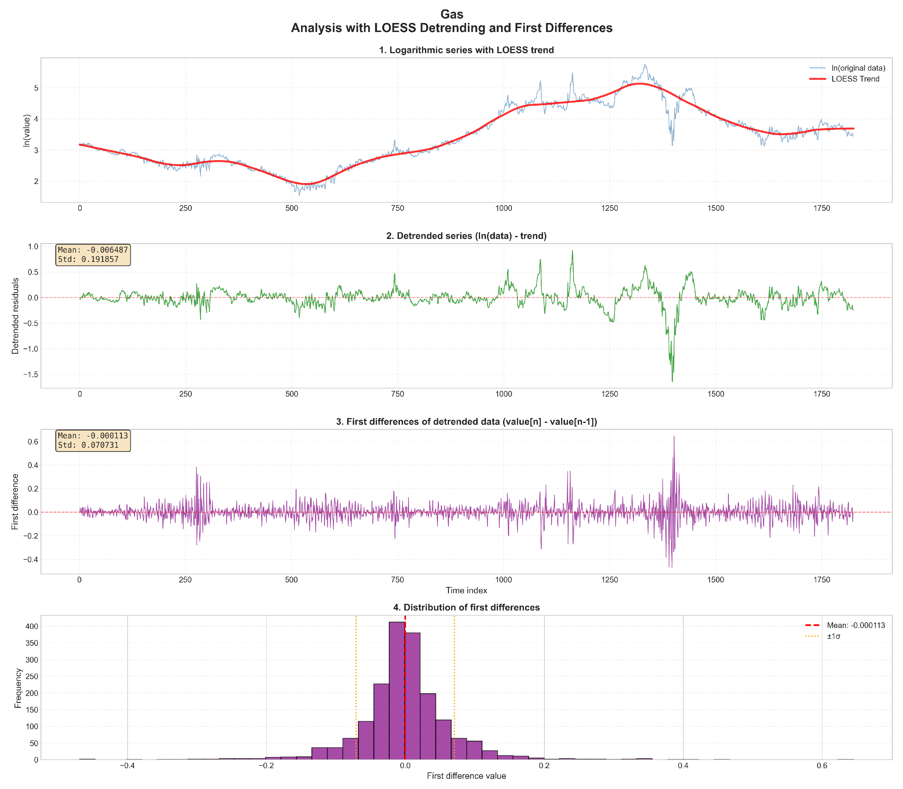
Figure 2.
Preprocessing pipeline for power: (a) logarithmic transformation with LOESS trend, (b) detrended series, (c) log-returns, (d) histogram of log-returns.
Figure 2.
Preprocessing pipeline for power: (a) logarithmic transformation with LOESS trend, (b) detrended series, (c) log-returns, (d) histogram of log-returns.
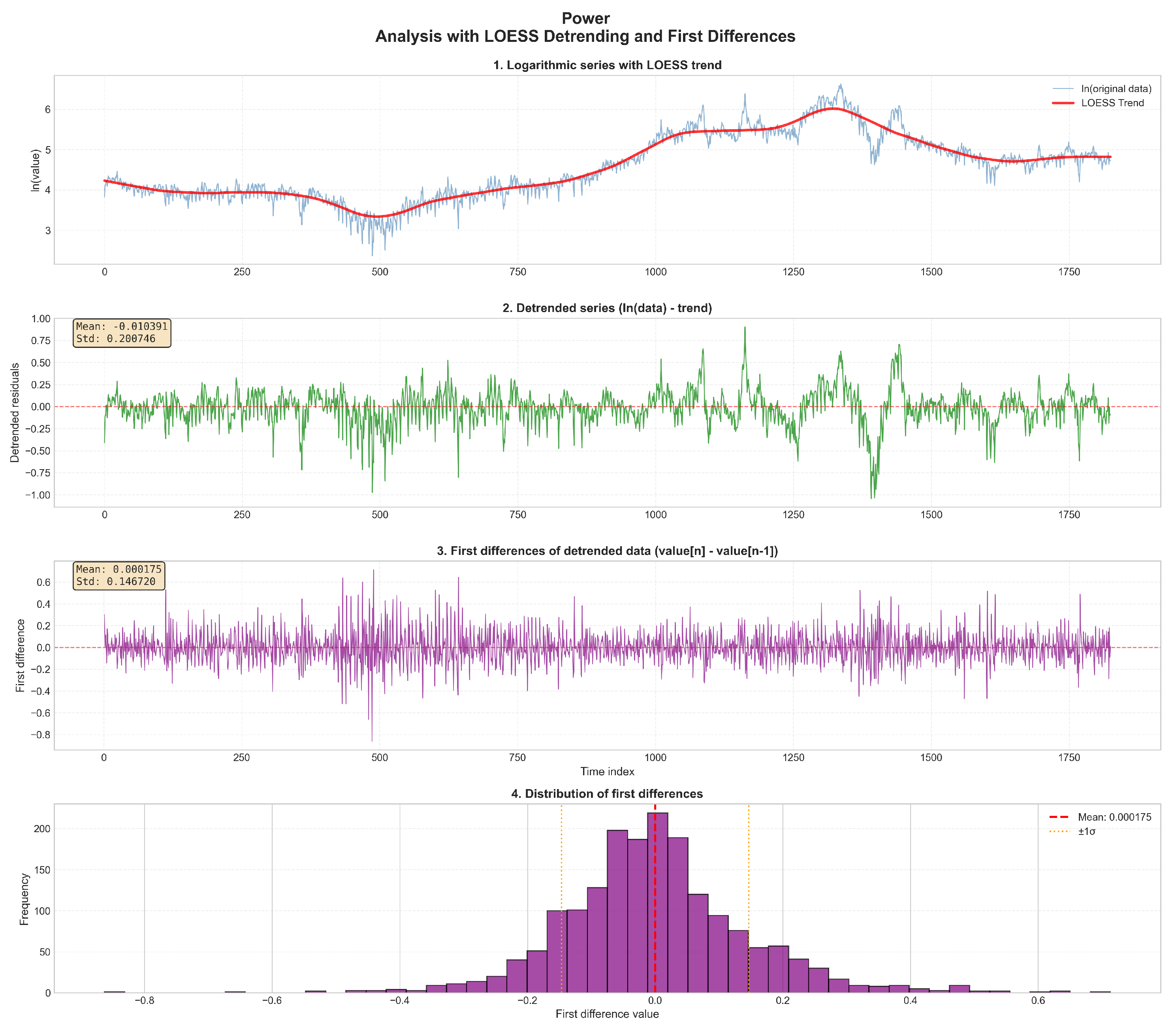
Figure 3.
Comparison of log-returns for gas (blue) and power (red). Power shows higher typical volatility, but gas exhibits more pronounced extreme events.
Figure 3.
Comparison of log-returns for gas (blue) and power (red). Power shows higher typical volatility, but gas exhibits more pronounced extreme events.
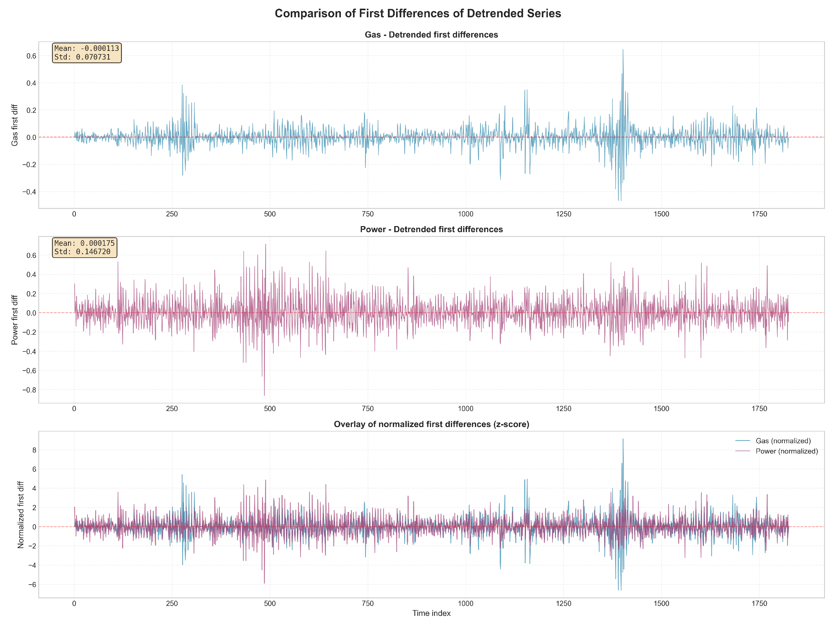
Figure 4.
Visibility graph connections for a gas log-return window (observations 500-1050). Red lines indicate visibility pairs. Note long-range connections spanning many observations, particularly involving extreme values.
Figure 4.
Visibility graph connections for a gas log-return window (observations 500-1050). Red lines indicate visibility pairs. Note long-range connections spanning many observations, particularly involving extreme values.
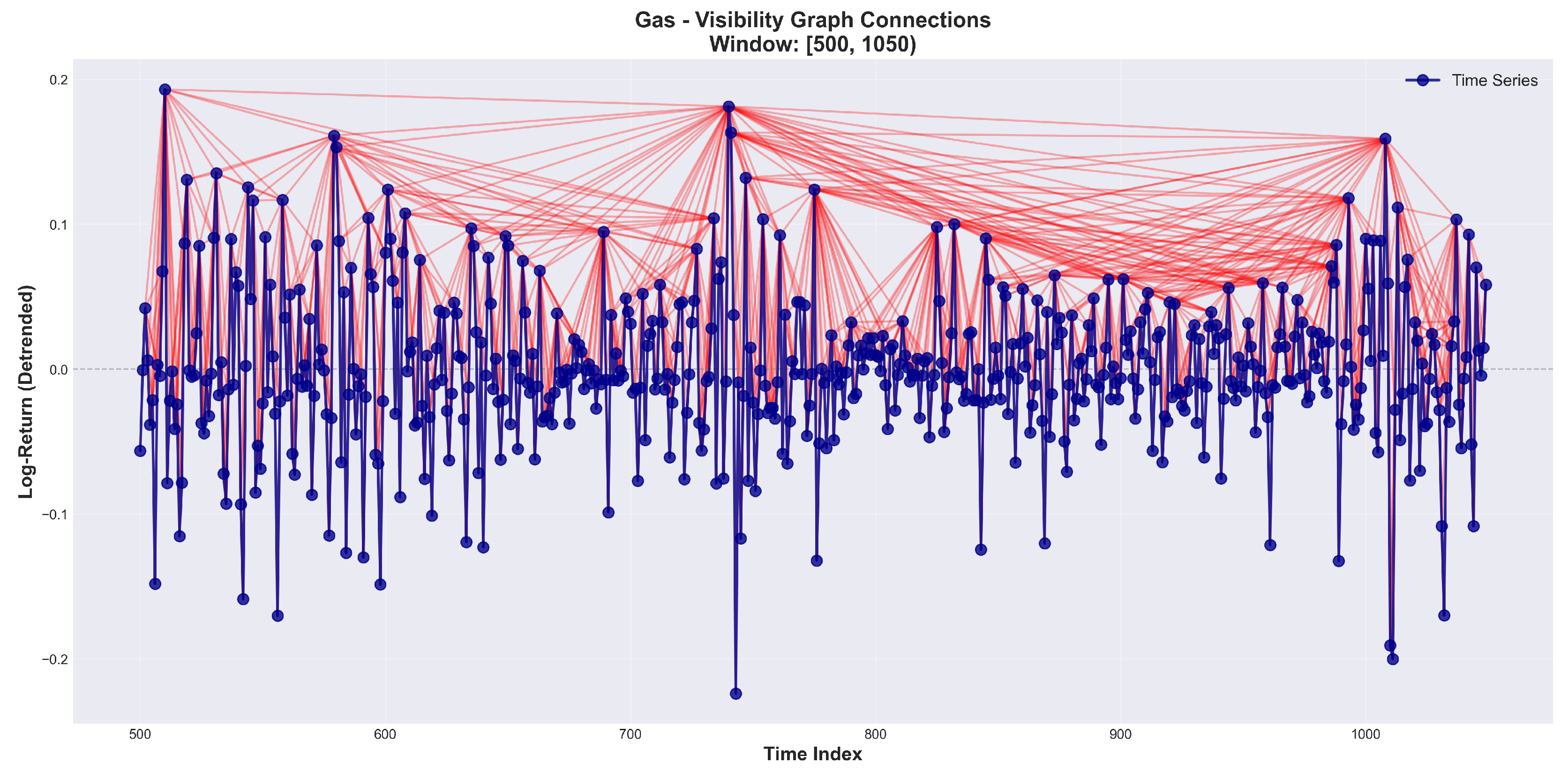
Figure 5.
Visibility graph connections for a power log-return window (observations 500-1050). Compared to gas, power exhibits fewer long-range connections despite higher volatility, suggesting different temporal correlation structure.
Figure 5.
Visibility graph connections for a power log-return window (observations 500-1050). Compared to gas, power exhibits fewer long-range connections despite higher volatility, suggesting different temporal correlation structure.
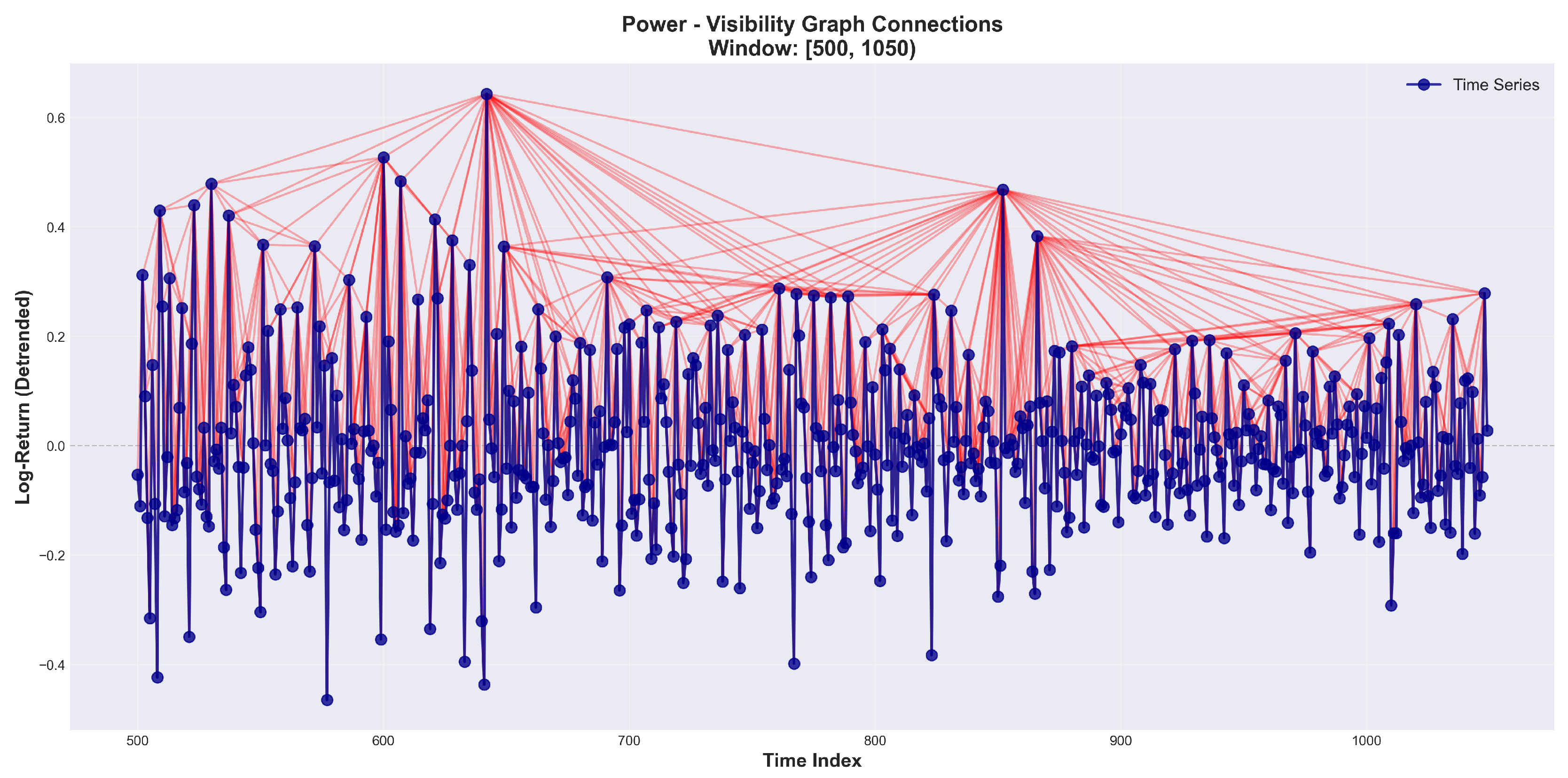
Figure 6.
Degree distributions for gas (a) and power (b) log-returns. Gas exhibits significantly heavier-tailed distribution extending to maximum degree 117, indicating strong hub nodes corresponding to persistent extreme events. Power shows more concentrated distribution with maximum degree 54, suggesting while power has higher raw volatility, extreme events are less persistent and create fewer long-range visibility connections.
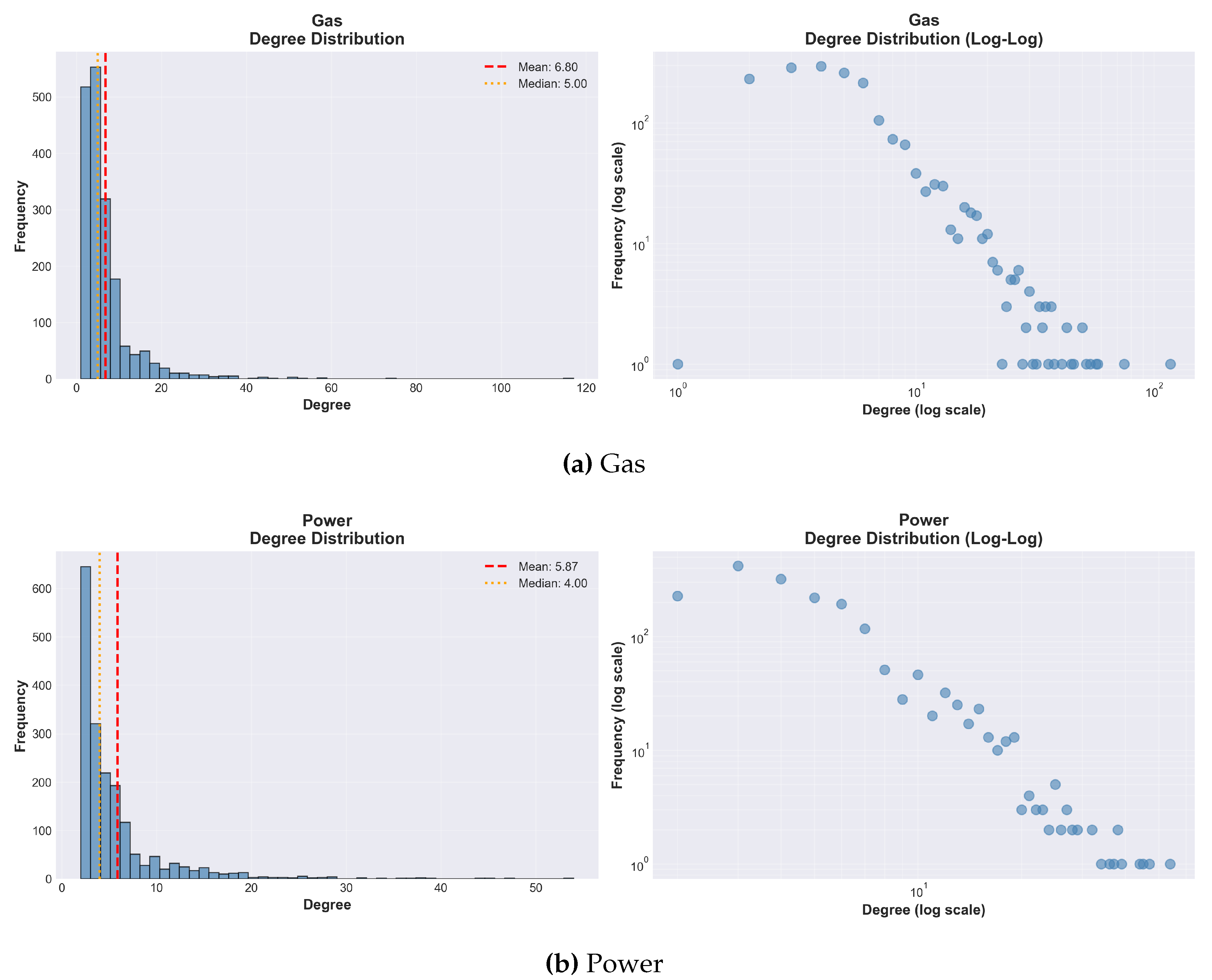
Figure 7.
Distribution of temporal distances between connected nodes for gas (blue) and power (red). Gas connections are substantially more evenly distributed across the full range of temporal distances, with significant probability mass extending to distances of 100-200 days or more. Power connections are heavily concentrated at short temporal distances (primarily 1-20 days) with rapid exponential decay. The different shapes reflect fundamentally different dynamical processes: gas exhibits persistent extreme events creating long-memory effects, while power displays more transient volatility with rapid mean reversion.
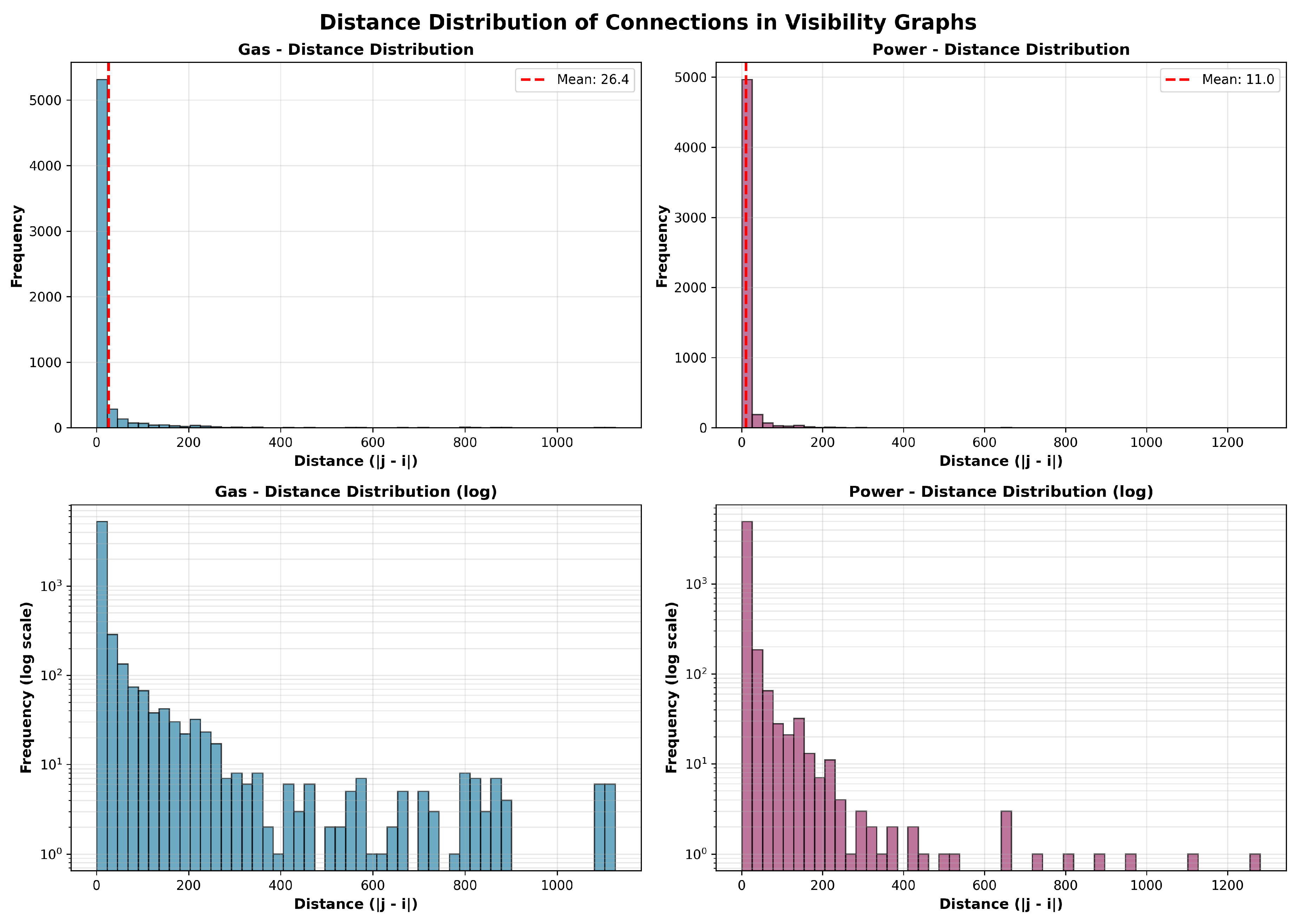
Figure 8.
Detailed visualization of visibility graph for gas log-returns (observations 200-250). Upper panel: Blue vertical lines represent time series values; red, orange, and purple lines indicate visibility connections at different distance ranges. Lower panel: Adjacency matrix where each cell indicates whether nodes i and j are connected (yellow/red = connection, dark blue = no connection). Note how extreme values create long-range connections spanning many time steps.
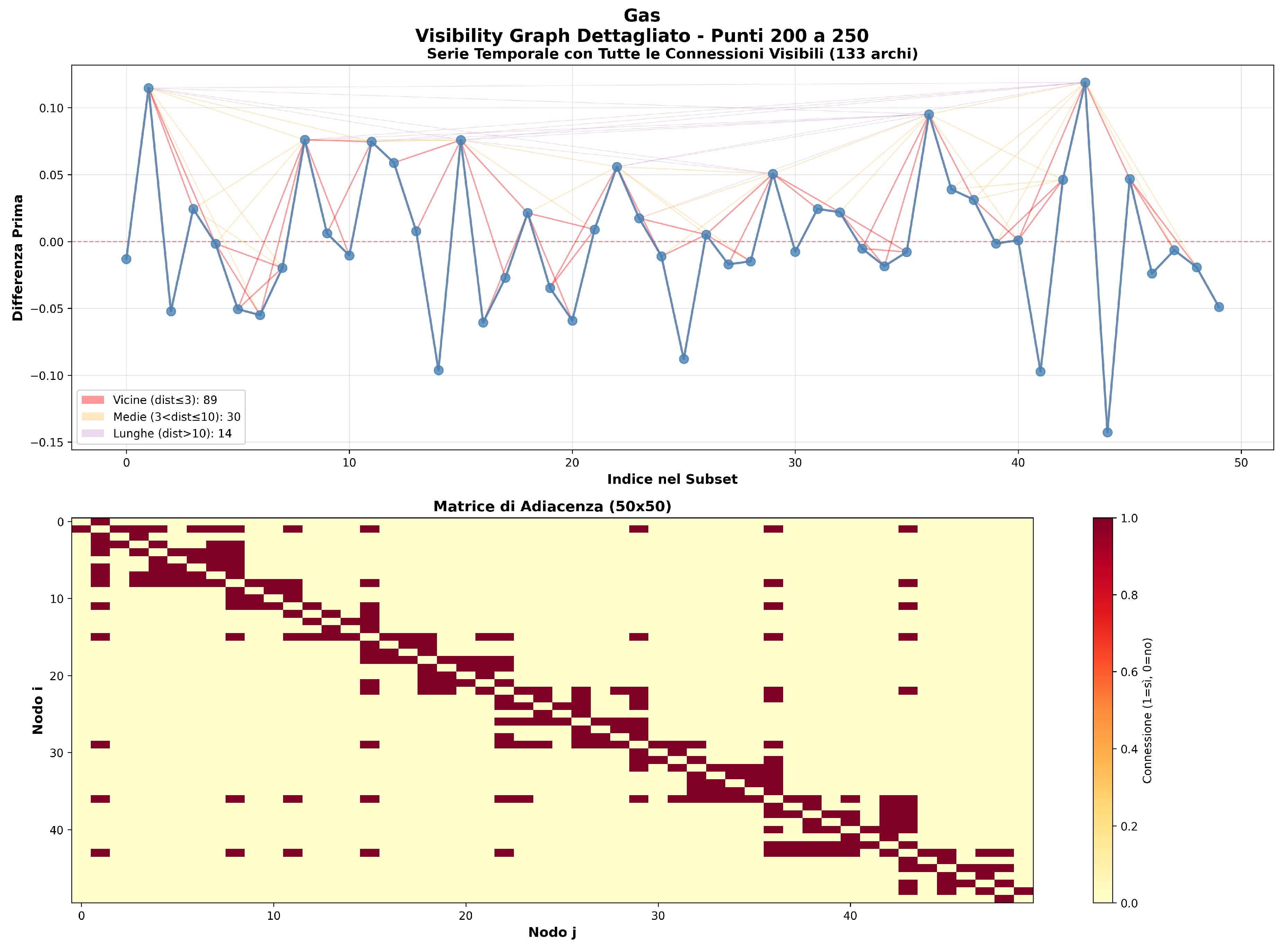
Figure 9.
Detailed visualization of visibility graph for power log-returns (observations 200-250). The structure reveals shorter-range connections compared to gas, reflecting rapid mean-reversion characteristic of power markets. The adjacency matrix shows more concentrated pattern near the diagonal, confirming local connection predominance.
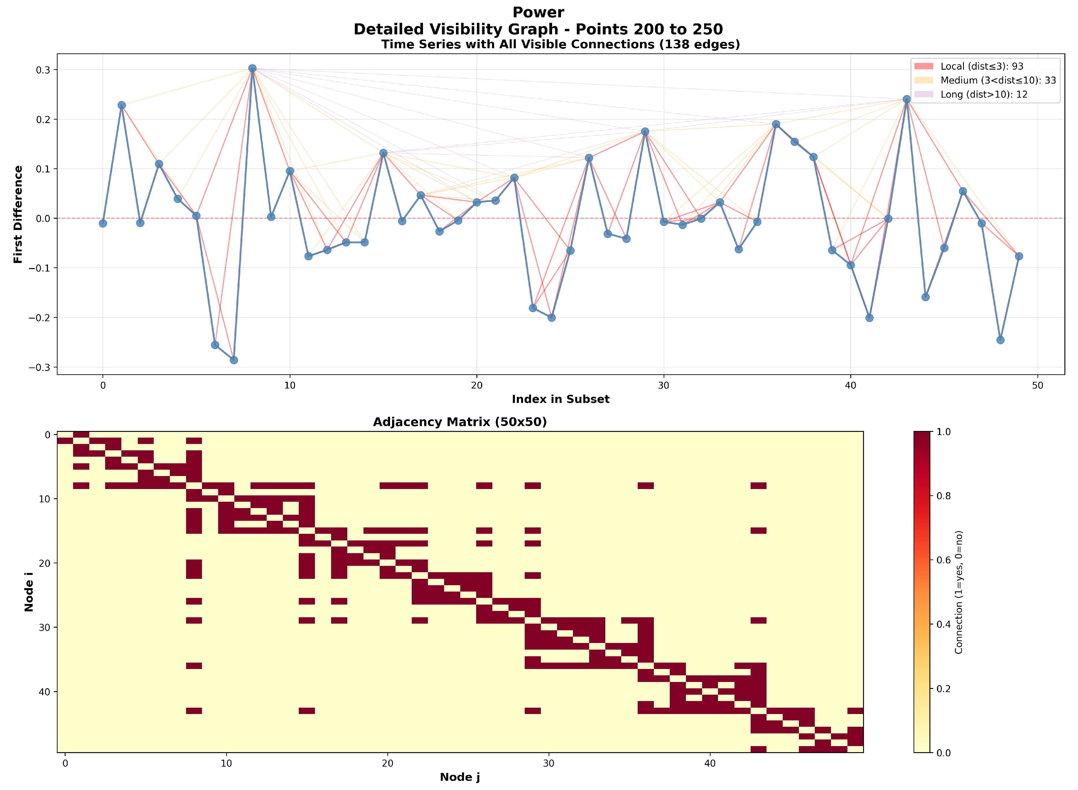
Figure 10.
Cross-correlation function between gas and power log-returns (bottom-right panel showing first differences). The sharp peak at lag = 0 with rapid decay to near-zero at all other lags confirms contemporaneous synchronization without systematic lead-lag relationships.
Figure 10.
Cross-correlation function between gas and power log-returns (bottom-right panel showing first differences). The sharp peak at lag = 0 with rapid decay to near-zero at all other lags confirms contemporaneous synchronization without systematic lead-lag relationships.
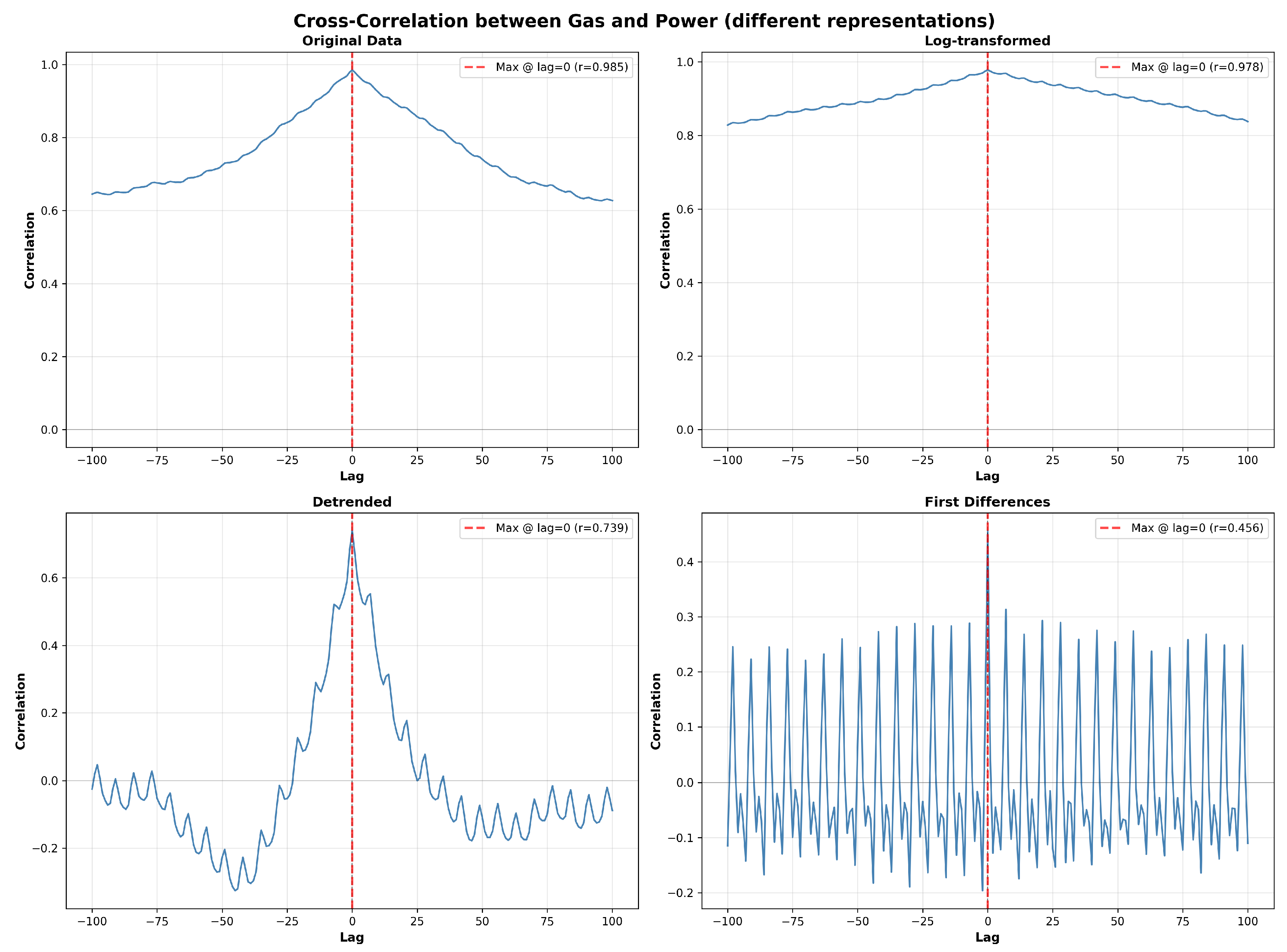
Figure 11.
Rolling correlation between gas and power log-returns computed over 100-day windows (bottom-right panel). Red dashed line indicates mean correlation (0.491); gray band shows standard deviation. The fluctuating pattern reveals regime changes in market coupling strength.
Figure 11.
Rolling correlation between gas and power log-returns computed over 100-day windows (bottom-right panel). Red dashed line indicates mean correlation (0.491); gray band shows standard deviation. The fluctuating pattern reveals regime changes in market coupling strength.
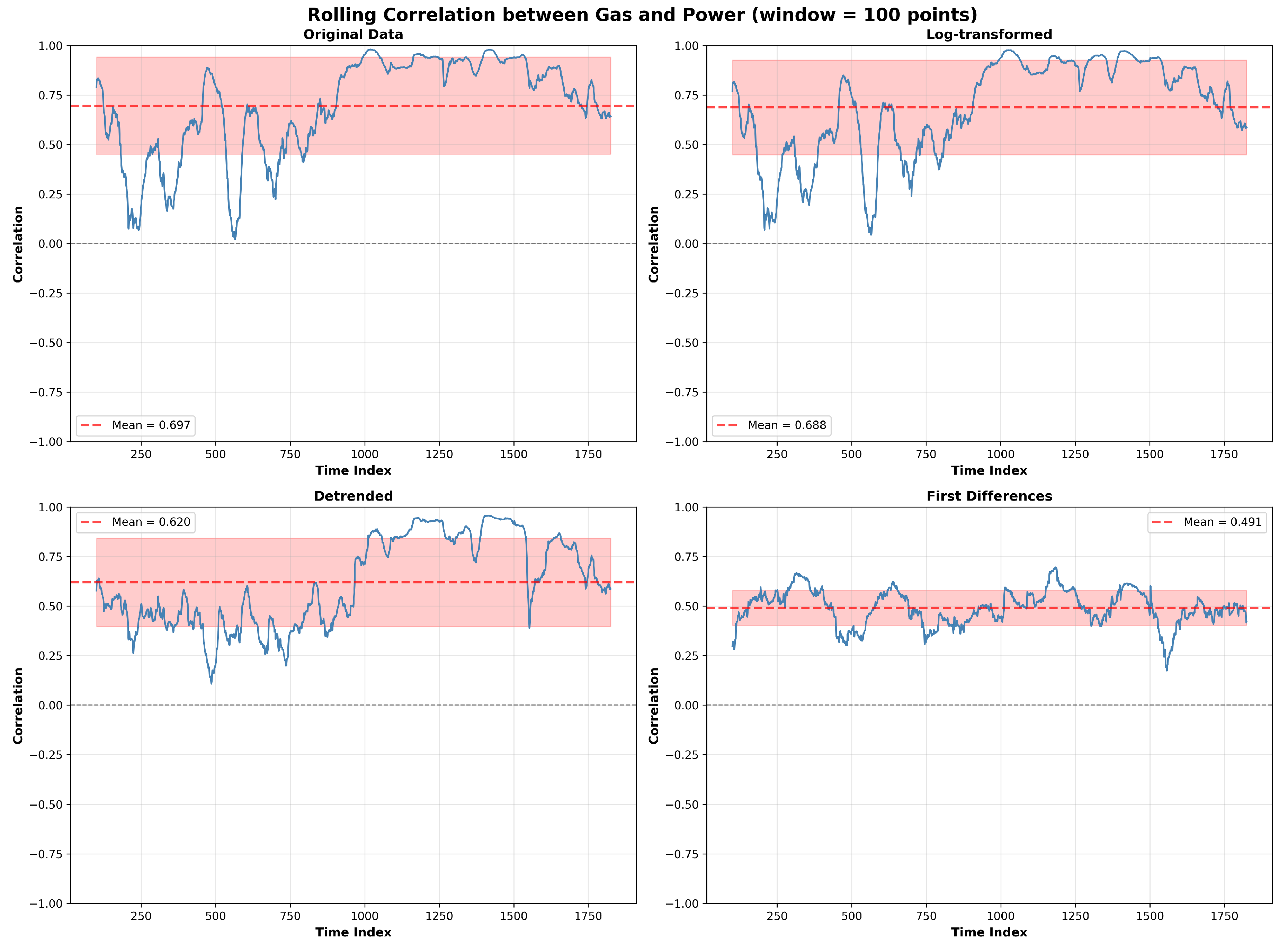
Figure 12.
Scatter plots showing correlations between node-level graph metrics from gas (horizontal axes) and power (vertical axes) visibility graphs. Top row: degree (left) and clustering coefficient (right) show positive correlations. Bottom row: betweenness centrality (left) shows no correlation; closeness centrality (right) shows strong negative correlation. Red dashed lines indicate fitted regressions.
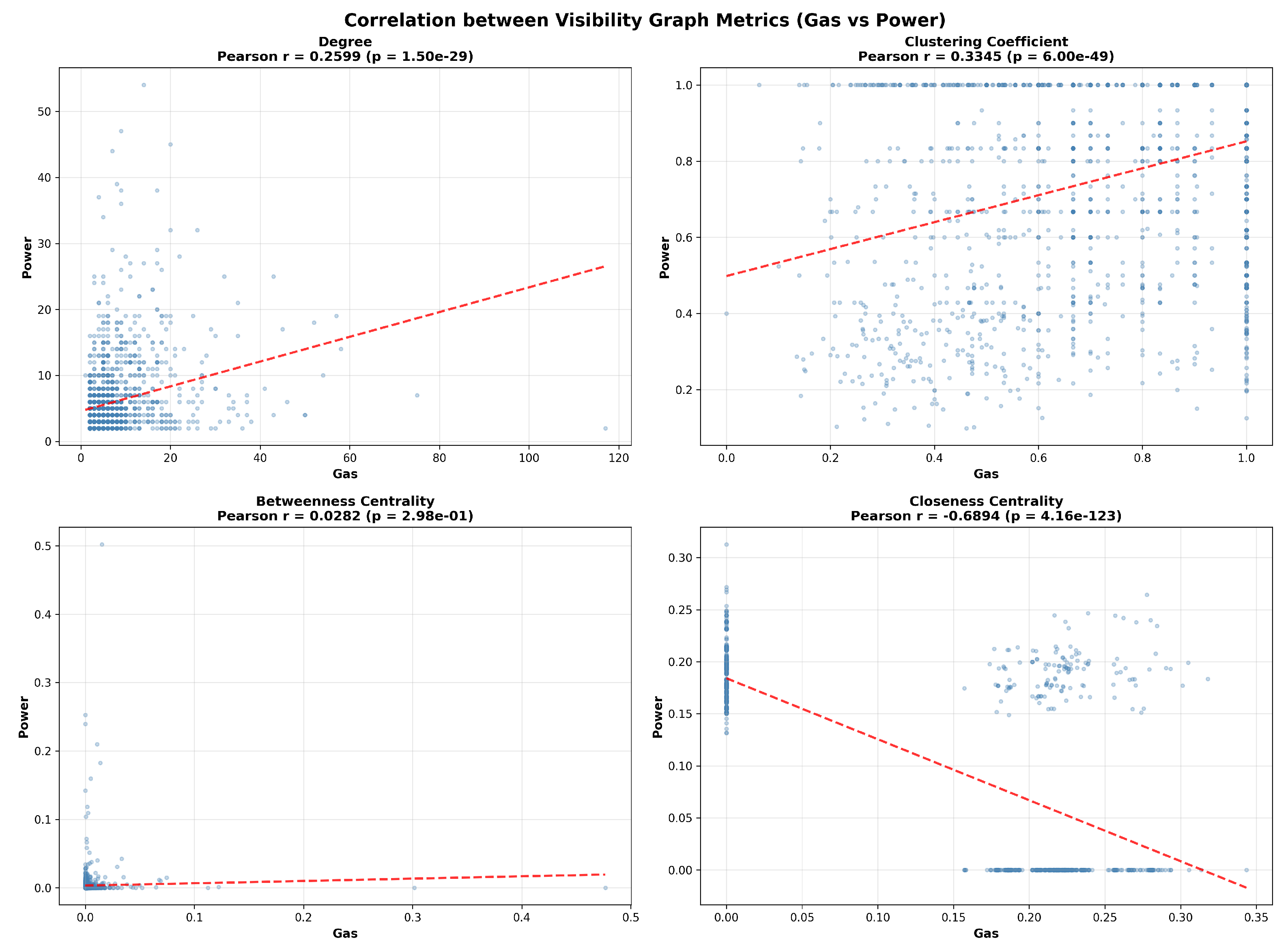

Table 1.
Topological properties of visibility graphs constructed from gas and power price first differences.
Table 1.
Topological properties of visibility graphs constructed from gas and power price first differences.
| Metric | Gas | Power |
|---|---|---|
| Number of nodes | 1,825 | 1,825 |
| Number of edges | 6,202 | 5,354 |
| Density | 0.003726 | 0.003217 |
| Average degree | 6.80 | 5.87 |
| Maximum degree | 117 | 54 |
| Clustering coefficient | 0.762 | 0.767 |
| Diameter | 9 | 10 |
| Average path length | 4.59 | 5.36 |
| Assortativity | 0.175 | 0.171 |
| Connected | Yes | Yes |
Table 2.
Temporal distance statistics for visibility graph edges.
| Distance Category | Gas | Power |
|---|---|---|
| Distance = 1 (adjacent points) | 29.41% | 34.07% |
| Distance = 2 | 14.90% | 17.99% |
| Distance = 3–4 | 16.98% | 18.45% |
| Average distance | 26.39 | 10.96 |
Table 3.
Correlation coefficients between gas and power log-returns. All p-values indicating statistical significance despite moderate correlation magnitude.
Table 3.
Correlation coefficients between gas and power log-returns. All p-values indicating statistical significance despite moderate correlation magnitude.
| Correlation Measure | Coefficient | p-value | Interpretation |
|---|---|---|---|
| Pearson r | 0.456 | Moderate positive linear correlation | |
| Spearman | 0.482 | Moderate positive rank correlation | |
| Kendall | 0.335 | Moderate concordance | |
| 0.208 | — | 21% shared variance |
Table 4.
Cross-correlation analysis results for log-returns showing optimal lag and maximum correlation. Lag = 0 indicates contemporaneous (same-day) correlation is strongest.
Table 4.
Cross-correlation analysis results for log-returns showing optimal lag and maximum correlation. Lag = 0 indicates contemporaneous (same-day) correlation is strongest.
| Metric | Value | Interpretation |
|---|---|---|
| Optimal Lag | 0 days | No lead-lag relationship |
| Maximum Correlation | 0.456 | Same-day synchronization |
| Correlation at Lag ±1 | 0.085, 0.091 | Negligible adjacent-day correlation |
| Correlation at Lag ±5 | 0.023, 0.019 | No weekly predictability |
Table 5.
Statistics of rolling log-return correlations computed over 100-day windows. The range from 0.173 to 0.696 indicates substantial time variation across market regimes.
Table 5.
Statistics of rolling log-return correlations computed over 100-day windows. The range from 0.173 to 0.696 indicates substantial time variation across market regimes.
| Statistic | Value | Interpretation |
|---|---|---|
| Mean Correlation | 0.491 | Average relationship strength |
| Standard Deviation | 0.089 | Moderate temporal variability |
| Minimum Correlation | 0.173 | Weakest coupling episode |
| Maximum Correlation | 0.696 | Strongest coupling episode |
| Range | 0.523 | Substantial regime variation |
Table 6.
Correlations between node-level topological metrics of gas and power visibility graphs. Positive correlations for local metrics (degree, clustering) indicate partial synchronization; negative correlation for closeness centrality is surprising.
Table 6.
Correlations between node-level topological metrics of gas and power visibility graphs. Positive correlations for local metrics (degree, clustering) indicate partial synchronization; negative correlation for closeness centrality is surprising.
| Graph Metric | Pearson r | p-value | Interpretation |
|---|---|---|---|
| Degree | 0.260 | Weak-moderate positive | |
| Clustering Coefficient | 0.335 | Moderate positive | |
| Betweenness Centrality | 0.024 | 0.376 | Not significant |
| Closeness Centrality | -0.719 | Strong negative |
Disclaimer/Publisher’s Note: The statements, opinions and data contained in all publications are solely those of the individual author(s) and contributor(s) and not of MDPI and/or the editor(s). MDPI and/or the editor(s) disclaim responsibility for any injury to people or property resulting from any ideas, methods, instructions or products referred to in the content. |
© 2026 by the authors. Licensee MDPI, Basel, Switzerland. This article is an open access article distributed under the terms and conditions of the Creative Commons Attribution (CC BY) license (http://creativecommons.org/licenses/by/4.0/).
Copyright: This open access article is published under a Creative Commons CC BY 4.0 license, which permit the free download, distribution, and reuse, provided that the author and preprint are cited in any reuse.


