
Submitted:
31 December 2025
Posted:
02 January 2026
You are already at the latest version
Abstract
Accurate modeling of outdoor Wi-Fi propagation in dense urban environments is essential for smart city connectivity. Deterministic ray-tracing techniques provide high-fidelity insight into multipath propagation but suffer from high computational cost and limited scalability in large 3D environments. This work investigates a hybrid approach that combines MATLAB-based ray-tracing simulations with Machine Learning to enable scalable Wi-Fi~7 network analysis. A large dataset is generated over a realistic simulated university campus, covering multiple frequency bands (2.4, 5, and 6~GHz), transmit power levels, and ray-tracing configurations with reflections and diffractions. Several regression models are evaluated, with emphasis on transformer-based architectures. Results show that the FT-Transformer accurately approximates ray-tracing outputs while reducing inference time from months to minutes. The proposed framework enables fast surrogate modeling of radio propagation and supports network planning and digital twin applications.
Keywords:
WiFi 7
; digital twin
; wireless multipath propagation
; ray-tracing
; FT-transformer
1. Introduction
Smart city infrastructures increasingly rely on dense and reliable wireless connectivity to support public services, large-scale Internet of Things (IoT) deployments, campus networks, and outdoor urban applications. In such scenarios, wireless propagation is inherently three-dimensional and strongly influenced by complex building geometry and spatial layout, as illustrated by the real-world campus environment considered in this study (Figure 1).
In this context, Wi-Fi has evolved beyond its traditional indoor role and has become a key access technology for urban-scale connectivity due to its cost efficiency, operation in unlicensed spectrum, and continuous evolution toward higher throughput and lower latency [1,2,3]. Recent studies emphasize that next-generation Wi-Fi systems are expected to play a complementary role to cellular technologies in smart cities by enabling flexible, high-capacity access in outdoor and semi-outdoor environments such as campuses, pedestrian zones, and transportation hubs [4,5].
Providing accurate insights into Wi-Fi coverage in such scenarios is challenging due to the inherently three-dimensional (3D) nature of urban environments. Buildings of varying heights, irregular layouts, vegetation, and street canyons significantly influence radio propagation through reflection, diffraction, and shadowing effects, resulting in strong spatial variability of signal strength and link quality. Simplified two-dimensional planning assumptions and empirical propagation models are therefore often insufficient to capture the dominant physical mechanisms governing outdoor Wi-Fi performance in dense urban areas [6,7,8].
Deterministic ray-tracing techniques are widely regarded as one of the most physically accurate approaches for modeling wireless propagation in complex 3D environments [6]. By explicitly simulating electromagnetic interactions between radio waves and surrounding structures, ray tracing enables detailed analysis of multipath propagation, frequency-dependent attenuation, and non-line-of-sight behavior [6,7]. The increasing availability of high-resolution geographic data, such as OpenStreetMap (OSM), has further facilitated the construction of large-scale, realistic 3D urban radio environments. Such simulation-based representations align closely with the concept of a digital twin, in which a virtual replica of the physical environment is used to analyze, predict, and optimize system behavior [9,10].
Despite their high fidelity, ray-tracing simulations suffer from two fundamental limitations. First, their computational cost grows rapidly with environmental complexity, carrier frequency, and the number of allowed reflections and diffractions, often requiring weeks or months of computation on powerful multi-core server infrastructures for exhaustive scenario exploration (see Appendix C) [6,11]. Second, large-scale experimental validation of ray-tracing results is typically infeasible in real urban deployments, as acquiring comprehensive measurements across millions of transmitter–receiver combinations and diverse propagation conditions is prohibitively expensive and logistically impractical [7,8]. As a result, ray tracing should not be interpreted as a direct substitute for measurements, but rather as a digital twin mechanism that enables controlled exploration of propagation phenomena that cannot be directly observed at scale.
While ray-tracing-based digital twins offer valuable physical insight, there remains a lack of comprehensive studies providing statistical and system-level understanding of outdoor Wi-Fi propagation in realistic 3D urban environments. Existing Wi-Fi literature predominantly focuses on indoor scenarios or protocol-level optimizations, with comparatively fewer works addressing outdoor propagation behavior across multiple frequency bands under realistic geometric conditions [1,6]. This gap is particularly relevant for modern Wi-Fi systems operating in higher frequency bands, where propagation is more sensitive to obstructions and multipath complexity.
Recent advances in Artificial Intelligence and Machine Learning provide a promising pathway to overcome the computational limitations of ray tracing. By learning directly from large ray-tracing-generated datasets, data-driven models can approximate complex propagation behavior with orders-of-magnitude lower computational cost at inference time [1,12,13]. In particular, transformer-based architectures have demonstrated superior performance on structured and tabular data by modeling global feature dependencies through self-attention mechanisms [14,15]. In wireless communication research, attention-based models have shown strong potential for channel modeling and radio map generation, enabling fast and scalable prediction of spatial signal characteristics [12,13].
Motivated by these developments, this paper proposes a smart city–oriented digital twin framework for 3D outdoor Wi-Fi analysis that combines large-scale ray-tracing simulations with Transformer-based Machine Learning models. Using a detailed OSM-derived 3D (geographic) model of the Politehnica University of Timișoara campus and surrounding urban areas, we generate an extensive dataset capturing realistic outdoor Wi-Fi propagation across multiple frequencies, transmission powers, and propagation complexities (see Appendix A). We further demonstrate that Transformer-based models can accurately learn the underlying ray-tracing behavior, enabling the generation of detailed Wi-Fi propagation estimates in seconds, what would otherwise require weeks or months of simulation time on high-performance computing infrastructure (such as that presented in Appendix C).
The main contributions of this work are summarized as follows:
- A comprehensive 3D outdoor Wi-Fi coverage analysis focused on smart city and campus-scale environments;
- A ray-tracing-based digital twin framework for exploring propagation phenomena that are impractical to measure directly;
- A large-scale dataset capturing millions of transmitter–receiver interactions across multiple frequencies and propagation conditions;
- A transformer-based surrogate modeling approach that accurately approximates ray-tracing outputs with near-instantaneous inference;
- A unified framework bridging physically grounded simulation and AI-driven acceleration for scalable wireless network planning.
2. Related Work
Research related to this work spans four main directions: (i) the evolution of Wi-Fi technologies toward Wi-Fi 7 and their role in smart city environments, (ii) deterministic ray-tracing techniques for wireless propagation modeling, (iii) digital twin concepts for wireless networks, and (iv) machine learning approaches for channel modeling and radio propagation prediction. This section reviews representative works in each area and positions the contribution of this paper within the existing literature.
2.1. Wi-Fi Evolution and Smart City Connectivity
The IEEE 802.11 family of standards has evolved continuously to address increasing demands for throughput, latency reduction, and spectral efficiency. Recent surveys and technical analyses describe the transition from Wi-Fi 6/6E to Wi-Fi 7 (IEEE 802.11be), highlighting features such as ultra-wide 320 MHz channels, 4096-QAM modulation, multi-link operation, and enhanced multi-user coordination [2,16,17]. These advancements position Wi-Fi 7 as a key enabler for high-capacity wireless access in dense environments, complementing cellular technologies in smart city deployments.
Beyond physical-layer improvements, several studies emphasize the growing role of Wi-Fi in smart cities and large-scale outdoor scenarios, including campuses, transportation hubs, and public spaces. Szott et al. [1] provide a comprehensive survey on the application of machine learning to IEEE 802.11 systems, noting that most existing work focuses on indoor environments and protocol optimization, with limited attention given to outdoor propagation and spatial coverage analysis. This observation motivates further investigation into realistic outdoor Wi-Fi behavior under complex urban geometries.
2.2. Ray-Tracing Techniques for Wireless Propagation Modeling
Deterministic ray tracing has long been recognized as one of the most accurate approaches for modeling wireless propagation in complex environments. Classical works by Fuschini et al. [6] and Yun and Iskander [7] provide detailed overviews of ray-tracing principles, acceleration techniques, and practical applications in indoor and small-cell scenarios. These studies demonstrate the ability of ray tracing to capture multipath effects, non-line-of-sight propagation, and frequency-dependent attenuation with high physical fidelity.
Ray tracing has also been applied to more advanced wireless systems, including coordinated multi-point transmission [8], reconfigurable intelligent surfaces, and satellite-to-ground communications [18]. More recently, simulation platforms such as WiThRay [11] have been proposed to support flexible ray-tracing-based channel modeling in smart wireless environments. Despite these advances, the computational complexity of ray tracing remains a fundamental limitation, particularly in large-scale 3D urban environments and at higher frequencies. As a result, exhaustive ray-tracing simulations are generally confined to offline studies and a limited subset of the full parameter space, since exploring all combinations of frequencies, transmitter locations, and propagation conditions is computationally prohibitive.
2.3. Digital Twins for Wireless Networks
The concept of a digital twin has gained increasing attention as a means of integrating physical modeling, data, and analytics into a unified virtual representation of complex systems. In the context of wireless communications, digital twins enable simulation-driven analysis and optimization of network behavior without relying solely on costly real-world experimentation. Recent works highlight the potential of digital twins for network planning, performance prediction, and adaptive management in future wireless systems.
Ray-tracing-based digital twins have been proposed as a foundation for modeling radio environments with high physical accuracy, particularly when combined with detailed geographic information systems. However, existing digital twin implementations often suffer from scalability limitations due to the computational cost of repeated high-fidelity simulations. This challenge is especially pronounced in outdoor urban scenarios, where large spatial extents and complex geometries significantly increase simulation time. Consequently, recent research has focused on combining accurate physics-based simulations with Machine Learning models that learn to approximate ray-tracing results, enabling fast and scalable analysis once the models are trained [6,7,11,12,13].
2.4. Machine Learning and Transformer-Based Channel Modeling
To mitigate the computational burden of traditional propagation modeling, numerous studies have explored Machine Learning approaches for wireless channel prediction and radio map generation. Early work focused on classical regression techniques and ensemble methods, while more recent research has adopted deep learning architectures to capture nonlinear propagation effects. Chen et al. [12] introduced Radio Transformer Networks, demonstrating that attention mechanisms can effectively learn channel characteristics from data. Similarly, Xu et al. [13] proposed a Transformer-based neural radio map framework for fast channel prediction.
In parallel, Transformer architectures specifically designed for tabular and structured data have shown strong performance across a range of applications. The TabTransformer [14] and FT-Transformer [15] models leverage self-attention to capture global dependencies between features, making them well suited for learning complex relationships in structured datasets such as ray-tracing outputs. While these models have been validated on benchmark tabular datasets, their application to large-scale outdoor Wi-Fi propagation modeling remains relatively unexplored.
2.5. Positioning of This Work
In contrast to prior studies, this work focuses explicitly on outdoor Wi-Fi propagation in realistic 3D urban environments relevant to smart city deployments. By combining large-scale ray-tracing simulations with Transformer-based surrogate modeling, the proposed framework bridges the gap between physically grounded digital twins and scalable data-driven prediction. Unlike purely simulation-based approaches, our method enables near-instantaneous inference once trained, while preserving interpretability through physically meaningful input features. This positions the proposed approach as a practical solution for accelerating Wi-Fi planning and analysis in complex outdoor environments.
3. Theoretical Foundation
3.1. IEEE 802.11 Standard Evolution
The IEEE 802.11 standard, commonly known as Wi-Fi, has undergone significant evolution since its inception in 1997. Initially designed for basic wireless LAN communication, each new generation has improved spectral efficiency, throughput, latency, and support for modern applications. Figure 2 summarizes the major milestones in Wi-Fi evolution.
- 802.11 / Wi-Fi 1 (1997): The original Wi-Fi standard, operating in the 2.4 GHz band, with speeds up to 2 Mbps.
- 802.11a/b / Wi-Fi 2 (1999): Introduced higher speeds (up to 54 Mbps) using OFDM in the 5 GHz band (802.11a), and a more cost-effective 11 Mbps 2.4 GHz option (802.11b).
- 802.11g / Wi-Fi 3 (2003): Combined the speed of 802.11a with the range and compatibility of 802.11b in the 2.4 GHz band.
- 802.11n / Wi-Fi 4 (2009): Added MIMO (multiple input, multiple output) antennas, channel bonding, and dual-band support for higher throughput and reliability.
- 802.11ac / Wi-Fi 5 (2013): Enhanced MIMO and introduced MU-MIMO and wider channels (up to 160 MHz), offering Gbps-level throughput.
- 802.11ax / Wi-Fi 6 (2019): Focused on high-density environments with OFDMA, uplink MU-MIMO, and target wake time (TWT) for better efficiency and power saving.
- 802.11be / Wi-Fi 7 (2024): Aims to deliver extremely high throughput (EHT) using 320 MHz channels, 4096-QAM modulation, and Multi-Link Operation (MLO), supporting demanding applications such as AR/VR, 8K streaming, and real-time cloud gaming.
The evolution of IEEE 802.11 standards reflects a growing need for higher bandwidth, lower latency, and better spectrum utilization, especially in high-density urban and indoor environments. Wi-Fi 6 and Wi-Fi 7 play a crucial role in enabling next-generation applications like industrial automation, wireless AI inference, and massive IoT deployments.
3.2. Advanced Modulation Schemes in Wi-Fi Standards
Modern Wi-Fi standards rely on advanced modulation techniques to increase spectral efficiency and boost data throughput. Quadrature Amplitude Modulation (QAM) allows a wireless signal to carry more bits per symbol by encoding both amplitude and phase information.
- Wi-Fi 4 (802.11n) introduced support for up to 64-QAM, encoding 6 bits per symbol.
- Wi-Fi 5 (802.11ac) expanded this to 256-QAM (8 bits/symbol).
- Wi-Fi 6 (802.11ax) implemented 1024-QAM (10 bits/symbol), improving peak data rates by over 25%.
- Wi-Fi 7 (802.11be) pushes the boundary further with 4096-QAM, encoding 12 bits per symbol.
While higher-order QAM schemes significantly increase capacity, they also demand:
- Higher signal-to-noise ratio (SNR) at the receiver,
- Precise channel estimation,
- And minimal distortion from multipath effects.
As shown in Figure 3, each increase in modulation order results in a denser constellation diagram, making it more sensitive to signal degradation caused by fading, interference, and environmental complexity. This directly motivates the need for accurate channel prediction techniques, particularly in Wi-Fi 7 environments, where the use of 4096-QAM imposes strict reliability constraints on signal quality.
3.3. Modulation Principles and QAM Fundamentals
Quadrature Amplitude Modulation (QAM) is widely used in wireless communication standards, including Wi-Fi 6 and Wi-Fi 7, to increase data rates by encoding multiple bits per symbol. QAM modulates both the amplitude and the phase of a carrier wave, resulting in a two-dimensional constellation of unique symbols. Each symbol represents a distinct binary sequence, allowing more bits to be transmitted in each baud (symbol period).
The left side of Figure 4 illustrates how a higher bit rate can be achieved by transmitting more bits per symbol at a fixed baud rate. The right side shows constellation diagrams for various QAM levels, highlighting the increasing symbol density and the corresponding need for higher signal-to-noise ratio (SNR) and more accurate channel prediction as modulation complexity increases.
Table 1 summarizes key characteristics of common QAM schemes used across Wi-Fi generations, including the required SNR under typical conditions and the bits carried per symbol.
3.4. Channels and Bandwidths in Wi-Fi Evolution
A foundational improvement in modern Wi-Fi standards lies in the expansion of available frequency bands and channel bandwidths. Wi-Fi signals are transmitted over defined channels, which occupy portions of the electromagnetic spectrum. The bandwidth of a channel (measured in MHz) determines how much data can be carried per transmission interval.
Earlier generations such as Wi-Fi 4 and Wi-Fi 5 supported 40 MHz and 80 MHz channel widths, respectively. Wi-Fi 6 expanded this to 160 MHz, significantly improving capacity and performance. The most recent advancement, Wi-Fi 7 (802.11be), introduces 320 MHz ultra-wide channels, allowing devices to transmit more data simultaneously and enabling maximum theoretical speeds of up to 46 Gbps, nearly five times that of Wi-Fi 6.
Figure 5 provides an intuitive visualization of this bandwidth evolution. Wider channels are metaphorically illustrated as multilane highways supporting faster vehicles, rockets for Wi-Fi 7, cars for Wi-Fi 6, bicycles for Wi-Fi 5, and pedestrians for Wi-Fi 4, reflecting increasing data transport capacity.
In addition to bandwidth, newer Wi-Fi standards take advantage of expanded frequency bands. Wi-Fi 4 and 5 primarily use the 2.4 GHz and 5 GHz bands, which are increasingly congested with legacy devices (e.g., Bluetooth, microwaves, older Wi-Fi). Wi-Fi 6E introduced the 6 GHz band, and Wi-Fi 7 fully exploits it, offering cleaner spectrum, minimal interference, and multiple contiguous 160 or 320 MHz channels for high-throughput, low-latency wireless communication. This combination of broader channels and cleaner spectrum is essential for next-generation applications such as AR/VR, cloud gaming, and wireless AI workloads.
3.4.1. 2.4 GHz Wi-Fi Channels
The 2.4 GHz band represents the earliest and most widely deployed spectrum for Wi-Fi communications. In most regulatory domains, this band spans approximately 83.5 MHz, from 2.400 GHz to 2.4835 GHz, and is divided into 14 partially overlapping channels with center frequencies spaced 5 MHz apart. Despite the apparent availability of multiple channels, the effective usable spectrum is limited by the bandwidth requirements of Wi-Fi transmissions.
Traditional IEEE 802.11b systems employed direct-sequence spread spectrum (DSSS) with a channel bandwidth of approximately 22 MHz, while later standards such as IEEE 802.11g and IEEE 802.11n adopted orthogonal frequency-division multiplexing (OFDM) with an effective bandwidth of 20 MHz. As a consequence, adjacent channels in the 2.4 GHz band overlap significantly, leading to both adjacent-channel interference (ACI) and co-channel interference (CCI) when multiple access points operate in close proximity.
Figure 6 illustrates the channel structure of the 2.4 GHz band and highlights the overlap between neighboring channels. Due to this overlap, only a limited set of non-overlapping channels, typically channels 1, 6, and 11 in most regions, can be deployed simultaneously without causing severe interference. While co-channel interference can be partially mitigated through carrier sense multiple access with collision avoidance (CSMA/CA), adjacent-channel interference is particularly detrimental, as overlapping transmissions are not coordinated by the medium access protocol.
The high susceptibility of the 2.4 GHz band to interference significantly constrains network capacity and spatial reuse in dense deployments, especially in outdoor and campus-scale environments. As a result, performance in the 2.4 GHz band is often limited not by signal strength alone, but by interference dynamics arising from channel overlap and shared medium access.
3.4.2. 5 GHz Wi-Fi Channels
The expansion of Wi-Fi into the 5 GHz band significantly increased the amount of available spectrum compared to the 2.4 GHz ISM band, enabling a larger number of channels and wider channel bandwidths. Figure 7 provides an overview of the 5 GHz Wi-Fi spectrum, illustrating channel allocation across the Unlicensed National Information Infrastructure (U-NII) sub-bands, including U-NII-1, U-NII-2, U-NII-2e, and U-NII-3, as well as the presence of Dynamic Frequency Selection (DFS)–regulated frequencies.
As shown in Figure 7, the 5 GHz band supports a substantially higher number of non-overlapping channels for 20 MHz operation, which improves spatial reuse and reduces interference in dense deployments. Building on this increased spectral availability, channel bonding mechanisms introduced in IEEE 802.11n and extended in IEEE 802.11ac allow multiple adjacent channels to be combined, enabling bandwidths of 40 MHz, 80 MHz, and, in some configurations, 160 MHz.
However, the use of wider channels in the 5 GHz band introduces additional regulatory and operational constraints. A significant portion of the spectrum is subject to DFS requirements, which are intended to protect incumbent radar systems. Access points operating on DFS channels must perform channel availability checks and may be required to vacate channels upon radar detection, introducing delays and potential channel instability. As a result, despite the increased bandwidth compared to the 2.4 GHz band, effective channel availability in the 5 GHz band can be reduced in practice, particularly in outdoor and campus-scale deployments.
Overall, the 5 GHz band represents an important intermediate step in Wi-Fi evolution, alleviating many of the interference limitations of 2.4 GHz deployments while introducing new planning challenges related to regulatory constraints and channel bonding.
3.4.3. 6 GHz Wi-Fi Channels
The opening of the 6 GHz band represents a major milestone in the evolution of Wi-Fi, providing a substantially larger and less congested spectrum compared to the legacy 2.4 GHz and 5 GHz bands. This spectrum expansion, introduced with Wi-Fi 6E and further extended in Wi-Fi 7, enables a dense and flexible channelization structure supporting both conventional and ultra-wide bandwidths. Figure 8 illustrates the channel allocation of the 6 GHz band, including actual channel numbers, center frequencies, and permissible channel widths across the U-NII-5, U-NII-6, U-NII-7, and U-NII-8 sub-bands.
As shown in Figure 8, the 6 GHz band supports a significantly larger number of non-overlapping 20 MHz channels, which can be aggregated to form wider channels of 40, 80, and 160 MHz without the extensive overlap constraints observed in lower-frequency bands. Most notably, the wide contiguous spectrum enables the use of 320 MHz channels, introduced with IEEE 802.11be (Wi-Fi 7), effectively doubling the maximum channel width supported by previous Wi-Fi generations.
The availability of such ultra-wide channels comes with important regulatory considerations. Depending on the region and deployment scenario, operation in the 6 GHz band may be restricted to low-power indoor (LPI) devices or may require automated frequency coordination (AFC) for standard-power access points. These constraints influence both channel availability and effective coverage, particularly in outdoor and campus-scale environments.
From a propagation perspective, the use of wider channels in the 6 GHz band shifts performance limitations away from spectral congestion toward environmental factors such as path loss, blockage, and multipath dispersion. While 320 MHz channels enable extremely high peak data rates, their practical performance is highly sensitive to three-dimensional urban geometry, reinforcing the need for accurate propagation modeling and data-driven digital twin approaches when analyzing next-generation Wi-Fi deployments.
3.5. Wireless Ray-Tracing
In wireless communication systems, the received power in a Line-of-Sight (LoS) scenario can be determined using the Friis transmission equation. This model provides a quantitative relationship between the transmitted power () and the received power (), considering the impact of the propagation environment and antenna characteristics. The received power is given by
where is the transmitted power, is the signal wavelength, is the transmitter–receiver separation, and and denote the transmitter and receiver antenna gains, respectively. The Friis model assumes free-space propagation with an unobstructed LoS path and therefore serves as a baseline for more complex propagation models.
In realistic outdoor and urban environments, however, wireless propagation is strongly influenced by interactions between electromagnetic waves and surrounding objects such as buildings, terrain, and vegetation. Ray-tracing techniques extend the LoS model by explicitly accounting for multipath propagation mechanisms, including specular reflections, diffractions around edges, and, in some cases, scattering from rough surfaces. Each propagation path is modeled as a ray that undergoes successive interactions with the environment before reaching the receiver.
For reflected paths, the received power contribution of the i-th ray can be expressed as
where is the total propagation distance of the ray, is the number of reflections encountered, and denotes the Fresnel reflection coefficient at the k-th interaction. The reflection coefficient depends on the angle of incidence, polarization, and electromagnetic properties of the reflecting surface, such as relative permittivity and conductivity.
Diffraction effects become significant when the direct path is partially or fully obstructed. In ray-tracing models, diffraction is commonly approximated using knife-edge or uniform theory of diffraction (UTD) formulations, which introduce an additional diffraction loss term. For a diffracted ray, the received power can be modeled as
where D is the diffraction coefficient, which captures the attenuation caused by wave bending around obstacles and depends on the geometry of the diffracting edge and the wavelength.
The total received power at a given receiver location is obtained by coherently or incoherently summing the contributions of all valid rays, including the LoS component (if present), reflected rays, and diffracted rays. In practice, many ray-tracing implementations compute the received power as
where denotes the number of propagation paths considered, limited by parameters such as the maximum number of reflections and diffractions allowed in the simulation.
By explicitly modeling these propagation mechanisms, ray tracing provides a physically grounded representation of wireless channels in complex three-dimensional environments. However, the computational complexity of evaluating a large number of rays and interactions grows rapidly with environmental detail and frequency, motivating the use of data-driven surrogate models to approximate ray-tracing outputs in large-scale digital twin simulations.
3.6. MATLAB Ray-Tracing Support
MATLAB provides built-in support for deterministic wireless ray-tracing through its RF Propagation and Antenna Toolboxes, enabling physically grounded modeling of radio propagation in complex three-dimensional environments. Based on geometrical optics (GO) and uniform theory of diffraction (UTD) principles, the ray-tracing framework explicitly models line-of-sight (LoS), reflected, and diffracted propagation paths between a transmitter and multiple receiver locations.
Figure 9 illustrates a representative ray-tracing scenario in an urban environment, where multiple propagation paths are generated between a transmitter and a receiver by accounting for reflections from building facades and diffraction around edges. Each ray corresponds to a distinct propagation path characterized by its total path length, number of reflections, number of diffractions, interaction materials, and geometric parameters such as angles of departure and arrival.
For each valid propagation path, MATLAB computes the associated path loss by combining free-space attenuation with interaction-specific losses introduced by reflections and diffractions. Reflections are modeled using Fresnel reflection coefficients derived from the electromagnetic properties of the interacting surfaces, such as relative permittivity and conductivity, while diffraction losses are calculated using UTD-based formulations. Material properties (e.g., concrete, glass, metal, vegetation) can be explicitly assigned to scene objects, allowing the ray-tracing model to capture environment-dependent attenuation effects.
In addition to path loss, MATLAB provides access to detailed per-ray metadata, including phase shifts, angles of arrival and departure, and interaction points. This information enables coherent or incoherent summation of multipath components at the receiver, as well as fine-grained analysis of multipath structure and angular dispersion. Simulation complexity is controlled through user-defined parameters such as the maximum number of reflections and diffractions considered, allowing a trade-off between physical accuracy and computational cost.
While MATLAB’s ray-tracing framework enables high-fidelity modeling of wireless propagation in realistic environments, the computational burden increases rapidly with scene complexity, frequency, and the number of allowed interactions. This limitation motivates the use of data-driven surrogate models capable of learning ray-tracing behavior from simulation data, enabling fast propagation prediction within large-scale digital twin environments.
3.7. Significance for Wi-Fi 7 Channel Prediction
The continuous evolution of IEEE 802.11 standards, culminating in the emergence of Wi-Fi 7 (802.11be), introduces unprecedented complexity in wireless channel behavior. With support for ultra-wide 320 MHz bandwidths, 4096-QAM modulation, multi-link operation (MLO), and low-latency scheduling, Wi-Fi 7 deployments demand highly accurate, real-time channel knowledge.
Traditional empirical or simplified propagation models may struggle to reflect the dynamic and high-resolution behavior of Wi-Fi 7 channels, especially in indoor or dense urban environments. Ray-tracing provides a physically accurate foundation for modeling such behavior, but remains computationally expensive and configuration-dependent.
To bridge this gap, our proposed method leverages supervised machine learning on ray-tracing-generated datasets to learn patterns in signal strength, path complexity, and interaction features. By doing so, we aim to develop a scalable and portable channel predictor that captures the frequency-, spatial-, and power-specific characteristics of Wi-Fi 7 environments without relying solely on repeated full-resolution simulations.
Thus, understanding the trajectory of IEEE 802.11 evolution is not just historical context, it is foundational for justifying the need for intelligent, data-driven wireless modeling in next-generation networks.
4. Materials and Methods
4.1. MATLAB Coverage Map Environment Setup
The MATLAB-based coverage map simulations were executed using MATLAB R2024a with the RF Toolbox, Antenna Toolbox, and Mapping Toolbox. This computational environment enables the visualization and analysis of radio coverage over geospatial data imported from OpenStreetMap (OSM), ensuring a reproducible and physically accurate framework for modeling Wi-Fi propagation within the Timișoara, Romania urban area.
The simulation workflow begins with the import of six OSM layers:
- timisoara_center.osm
- timisoara_north.osm
- timisoara_east.osm
- timisoara_south.osm
- timisoara_west.osm
- upt_campus.osm
representing the city’s central and peripheral districts, as well as the Politehnica University campus. Each dataset was read using MATLAB’s readgeotable() function with the buildingparts layer enabled. All individual maps were concatenated into a unified geotable, resulting in a 3D city model containing approximately 31,404 buildings. Material information (e.g., brick, concrete, metal, glass) was mapped to specific colors through a MATLAB dictionary to facilitate visual differentiation within the siteviewer. Loading and merging the complete geographic dataset (3D buildings) required approximately 20 minutes on the powerful simulation servers, due to the geometric complexity of the urban model.
A single transmitter (txsite) was placed at the Politehnica University Timișoara Campus location (45.746458° N, 21.227445° E), placed on top of Building O (Figure 1) to represent a local Wi-Fi Access Point (AP) or IoT gateway. The transmitter operated at a frequency of 2.4, 5, and 6 GHz with a power level of 100, 200, 500, or 1000 mW), and used a half-wave dipole antenna designed via design(dipole, f), mounted at a height of 5 m. The receiver sensitivity threshold was set to -90 dBm, corresponding to typical Wi-Fi device characteristics.
Signal propagation was modeled using the Shooting and Bouncing Rays (SBR) method through MATLAB’s propagationModel("raytracing") function. The model was configured to account for both reflections and diffractions, defined respectively by the parameters MaxNumReflections and MaxNumDiffractions. Coverage was computed using the coverage() function with a 350 m maximum range and 5 m spatial resolution. The signal strength levels were displayed between -90 dBm and -40 dBm, using a semi-transparent overlay for improved visual integration with the urban geometry.
The configuration space for the simulations is illustrated in Figure 10, where each cell represents a reflection–diffraction (R/D) combination. The setup supports repetition of these simulations for all relevant frequency bands (2.4 GHz, 5 GHz, and 6 GHz) and transmitter power levels (100 mW, 200 mW, 500 mW, and 1000 mW), thereby enabling multi-scenario evaluation of propagation characteristics under varying power and frequency conditions.
The coverage environment was rendered using the OpenStreetMap basemap within MATLAB’s siteviewer, allowing interactive inspection of 3D structures and ray interactions. Execution timestamps were logged at both start and completion using datetime(’now’) to ensure reproducibility and enable runtime benchmarking. This environment serves as the foundation for the subsequent receiver grid generation and RSSI regression modeling presented in Sections 4.2 and 4.3.
4.2. 3D Coverage Map Visualization Setup
To accurately represent signal propagation in an urban environment, a three-dimensional (3D) coverage map was generated using MATLAB’s siteviewer environment. The visualization integrates topographical data, building geometries, and radio coverage results to enable interactive exploration of the simulation domain. The rendering was based on the OpenStreetMap (OSM) basemap, which provides detailed building footprints, street layouts, and vegetation features of the Politehnica University of Timișoara campus and its surrounding areas.
The imported OSM datasets include six geospatial layers covering the central, northern, eastern, southern, western, and campus regions of Timișoara. Each layer was preprocessed with the readgeotable() function, focusing on the buildingparts attributes to extract building height and material information. The combined dataset resulted in a city-scale model of 31,404 buildings, which were rendered as 3D extrusions within the viewer.
The transmitter (txsite) was placed at coordinates 45.746458° N and 21.227445° E, at a height of 5 m above the building level. The antenna configuration was defined using the MATLAB function design(dipole, f) for each operational frequency. The propagation model used the propagationModel("raytracing") function configured for Shooting and Bouncing Rays (SBR) analysis. This level of complexity provides a balance between physical accuracy and computational efficiency for dense urban environments.
Signal strength values were computed using the coverage() function with parameters:
- SignalStrengths: [-90:5:-40]
- MaxRange: 350 m
- Resolution: 5 m
- Transparency: 0.6
The resulting power map (Figure 11) displays spatial variations in received signal strength across the area, where red areas correspond to strong signal coverage (-40 dBm to -60 dBm), and blue regions represent weak or obstructed reception (-90 dBm or lower). The visual output effectively correlates the influence of building density and material composition on signal attenuation and multipath effects.
This interactive 3D rendering allows for zooming, rotation, and ray inspection directly within the MATLAB environment, supporting deeper analysis of line-of-sight (LoS) and non-line-of-sight (NLoS) conditions. Consequently, the setup serves as a reliable testbed for validating propagation models under realistic urban conditions, which will be extended in subsequent sections to multi-frequency and multi-power scenarios.
4.3. Antenna Configuration and Theoretical Model
Figure 12 summarizes the transmitting antenna used throughout this study: a center-fed half-wave dipole designed in MATLAB for each operating band (2.4, 5.0, and 6.0 GHz) using design(dipole,f). The dipole was selected as a reference radiator because it provides a stable, well-understood omnidirectional azimuth response, making it suitable for isolating propagation effects (e.g., reflections/diffractions) from antenna-specific beamforming artifacts.
4.3.1. Geometric Scaling with Frequency
For an ideal half-wave dipole, the total length L scales with the free-space wavelength:
where c is the speed of light and f is the carrier frequency. Accordingly, the dipole geometry becomes shorter at higher frequencies (Figure 12, center), while maintaining the same electrical length and resonant behavior. In our simulations, MATLAB automatically adjusts the dipole dimensions to satisfy the half-wave resonance condition at each band, using a center feed that preserves symmetry and consistent polarization.
4.3.2. Radiation Characteristics and Implications for Coverage
A half-wave dipole exhibits a characteristic toroidal radiation pattern, with maximum radiation in the plane perpendicular to the antenna axis and nulls along the axis. This behavior is visible in Figure 12 (right), where the 3D pattern remains consistent across 2.4–6 GHz, and the azimuthal directivity cut (left) is close to uniform. Such a pattern is advantageous in outdoor access-point or gateway-like deployments where uniform horizontal coverage is desired.
4.3.3. Justification for Simulation Use
Using a dipole as the transmit antenna provides a controlled baseline for analyzing propagation phenomena in a 3D urban/campus environment, because link variability is dominated by geometry and material interactions rather than highly directive antenna patterns. Moreover, prior studies have experimentally validated comparable half-wave dipole designs for Wi-Fi/WLAN bands, reporting gains close to the theoretical dBi and radiation patterns consistent with analytical expectations [19,20]. Therefore, the MATLAB-generated dipole models offer a reproducible and physically meaningful antenna representation for the ray-tracing coverage simulations presented in this work.
4.4. MATLAB Data Collection Environment Setup
4.4.1. Circular Receiver Array Generation
The circular receiver array represents a spatially symmetric configuration of receiver nodes uniformly distributed around a central transmitter. This topology enables isotropic coverage assessment and facilitates comparative signal strength analysis across multiple azimuth directions. The deployment is particularly suited for propagation modeling and interference analysis, where identical receiver conditions are desired around a reference point.
The array geometry is defined by a circular perimeter of radius r, centered at the base transmitter coordinates . Each of the N receivers is placed at a constant angular separation of , ensuring uniform spatial distribution. The position of each receiver is computed along a great-circle trajectory on the Earth’s surface using the geodesic direct problem formulation, as can be seen in Equation 2.
The expression defined in Equation 2 defines the geographic coordinates of the i-th receiver along a circular array using a geodesic reckoning MATLAB function. This operation computes a new location on the Earth’s surface given a starting point, an angular distance, and an azimuthal bearing. The parameters involved are described as follows:
- : The latitude of the base (transmitter) site, expressed in degrees. This serves as the geodetic origin from which all receiver positions are derived.
- : The longitude of the base (transmitter) site, expressed in degrees. Together with , it defines the center of the circular array.
- : The angular distance (central angle) subtended by the circle at the Earth’s center, measured in degrees or radians. It is computed as described in Equation 3.where r is the desired linear radius of the circular array (in meters), and is the mean Earth radius (approximately ). This conversion ensures accurate great-circle positioning even at non-negligible distances.
- : The azimuth angle (or bearing) of the i-th receiver with respect to geographic north, measured clockwise in degrees. It determines the orientation of each receiver on the circular perimeter and is given by Equation 4.where N is the total number of receivers in the array.
- : The computed latitude and longitude of the i-th receiver site after applying the great-circle offset from the central transmitter.
In practical terms, the function in MATLAB uses a spherical Earth approximation to calculate the endpoint of a geodesic arc starting at , traveling a surface distance corresponding to , and following the azimuthal direction . This ensures that all receiver sites are evenly distributed around the central node along a true geodesic circle, accounting for Earth curvature rather than relying on planar projections.
This geodesic approach ensures accurate placement of receivers even over large distances or in non-planar terrain, maintaining consistency with Earth curvature effects. Each receiver node is modeled as a measurement site characterized by its geographic coordinates, antenna parameters, and receiver sensitivity. In this study, a half-wave dipole antenna tuned to the operating frequency f was used for each receiver to approximate an omnidirectional radiation pattern suitable for general-purpose coverage evaluation.
The configuration defines an altitude threshold that is later applied to filter out receivers positioned on top of buildings or other elevated structures. This parameter is not used during the initial array generation but serves as a post-processing criterion when populating a defined geographic area with receivers for data collection. By excluding high-elevation placements, the resulting receiver distribution remains representative of ground-level conditions, ensuring that signal measurements reflect realistic propagation environments within the selected coverage area.
The resulting array forms a geodesically uniform sampling grid surrounding the transmitter, enabling comprehensive assessment of received signal strength and coverage uniformity in all directions. The geometry of the array is illustrated in Figure 13, which presents a two-dimensional overhead view (left) and a three-dimensional perspective (right) of the deployed receiver nodes around the transmitter, generated using MATLAB’s Site Viewer.
This formulation provides a mathematically consistent and computationally efficient method for generating a circular array of receivers suitable for evaluating coverage, power distribution, and signal degradation as a function of azimuth, elevation, and distance from the transmitter.
4.4.2. Resolution-Driven Receiver Grid Filling via Concentric Circles
While the circular receiver array formulation in (2) establishes how a single ring of receivers can be placed around a transmitter, the practical dataset generation requires filling an entire area with receiver sites at a controllable spatial resolution. To achieve this, we implemented a resolution-driven sampling strategy that constructs multiple concentric circles around the transmitter and automatically adjusts the number of receivers per circle as a function of the desired receiver spacing. This produces an approximately uniform sampling density in the horizontal plane while preserving geodesic correctness.
A single parameter, denoted here by (in meters), defines both: (i) the radial spacing between successive circles, and (ii) the arc-length spacing between adjacent receivers on the same circle. In our experiments, typical values were , corresponding to coarse and dense receiver sampling, respectively.
Given a maximum coverage radius , the number of concentric circles is computed as:
so that circle k (with ) has radius:
For each circle of radius , the circumference is . The number of receivers on that circle is selected to keep the arc-length separation close to :
Receivers are then placed at uniformly spaced azimuth angles,
and converted to geographic coordinates using MATLAB’s great-circle reckoning:
where denotes the mean Earth radius.
Although the circle construction is centered at the transmitter, we only retain receivers that belong to a user-defined target area, specified as a latitude/longitude polygon. For each candidate receiver, we apply an inclusion test:
implemented with MATLAB’s inpolygon() function (note that inpolygon() expects the input order ). Receivers outside the polygon are discarded, which allows the concentric-circle generator to fill arbitrary footprints (rectangular, campus-shaped, or street-bounded regions) while maintaining near-uniform sampling density.
In addition, we optionally enforce an elevation constraint to avoid placing receivers on elevated rooftops or terrain outliers:
where is obtained via MATLAB’s elevation() query and is a user-defined limit (disabled when ).
The final receiver set is therefore:
Figure 14 illustrates the resulting receiver deployment over the campus area: the transmitter is centered in the region, and the receiver sites densely cover the polygon footprint using multiple rings. An inset view highlights how the grid density increases as decreases (e.g., vs. ), directly controlling the number of receivers and the total simulation workload.
This strategy enables controlled scaling of the dataset: reducing increases both the number of circles and the number of receivers per circle, leading to a rapid growth in total receiver count (and thus ray-tracing calls). Consequently, acts as the main knob for trading spatial fidelity against runtime and storage requirements, which is essential when generating millions of transmitter–receiver samples for subsequent machine learning regression.
4.5. Machine Learning Regression Strategy for RSSI Prediction
The objective of this study is to replace computationally expensive ray-tracing simulations with a data-driven surrogate model capable of accurately predicting the Received Signal Strength Indicator (RSSI) for Wi-Fi 7 links in a 3D urban environment. The regression task is formulated using ray-tracing outputs as ground-truth labels and aims to learn the functional relationship between transmitter–receiver geometry, propagation conditions, and received signal strength.
4.5.1. Problem Formulation
Let denote a dataset of n wireless links generated through ray-tracing simulations. Each input vector encodes the physical and geometric characteristics of the i-th transmitter–receiver pair, while the target value corresponds to the simulated RSSI expressed in dBm.
The feature vector aggregates parameters that are known to influence radio propagation, including but not limited to the three-dimensional transmitter–receiver distance, operating frequency, transmit power, antenna heights, relative azimuth and elevation angles, and ray-tracing descriptors such as the number of reflections and diffractions. These features collectively describe the propagation scenario without explicitly modeling the electromagnetic interactions.
The learning objective is to estimate a parametric regression function
where is a nonlinear function parameterized by , and denotes the predicted RSSI. The parameters are optimized by minimizing a regression loss over the dataset:
where is a suitable loss function, such as the mean squared error.
From a physical perspective, the function acts as a surrogate for the ray-tracing propagation model by implicitly learning the combined effects of free-space attenuation, reflection, diffraction, and material interactions encoded in the input features. Once trained, the surrogate model enables rapid RSSI prediction for unseen transmitter–receiver configurations, reducing inference time from minutes or hours per scenario to milliseconds while preserving high-fidelity spatial coverage characteristics.
4.5.2. Machine Learning Models
To approximate the ray-tracing propagation model, we evaluate several supervised regression approaches commonly used for structured and tabular data. Among these, the FT-Transformer is adopted as the primary model in this study due to its consistently superior predictive accuracy, training stability, and robustness across heterogeneous feature distributions. FT-Transformer extends transformer architectures to tabular regression by combining feature tokenization with self-attention, enabling it to capture complex nonlinear interactions between geometric, frequency-dependent, and propagation-related parameters.
For comparison, we also include the TabTransformer, which applies contextual embeddings to categorical and continuous features using self-attention, as well as a Random Forest Regressor representing classical ensemble-based machine learning. These models serve as strong baselines for assessing the benefit of attention-based architectures in learning high-dimensional propagation relationships.
In addition, selected gradient-boosting models such as LightGBM and XGBoost, as well as Convolutional Neural Network (CNN) variants adapted for structured inputs, are optionally evaluated to provide further reference points. However, the main emphasis of the analysis remains on FT-Transformer, as it demonstrates the most favorable trade-off between prediction accuracy, generalization capability, and training stability for large-scale RSSI regression tasks.
4.5.3. Transformer-Based Regression for RSSI Prediction
While ensemble tree methods and deep neural networks can accurately model nonlinear propagation effects, they are limited in their ability to capture long-range feature dependencies and contextual relationships between radio-environment variables. To overcome these limitations, we extended the regression framework with a transformer-based architecture capable of modeling feature interactions and spatial patterns relevant to the propagation process.
Transformers employ self-attention mechanisms that compute the contextual importance of each feature relative to others within a given sample. In the context of radio propagation, this allows the model to jointly reason about how parameters such as distance, frequency, transmitter height, and reflection count influence the received signal strength. Unlike convolutional or tree-based models, which primarily learn local or hierarchical relations, transformers learn global dependencies that generalize better across frequency bands, transmitter–receiver geometries, and urban layouts.
In terms of model architecture, we adopted a tabular transformer configuration inspired by the TabTransformer [14] and FT-Transformer [15] architectures. Each input feature was embedded into a d-dimensional vector space via a learnable linear projection:
where and are trainable parameters. The resulting set of feature embeddings forms a token sequence processed by a stack of L self-attention layers:
where MSA denotes multi-head self-attention, LN denotes layer normalization, and MLP represents a feed-forward network. The final contextual embeddings are aggregated through average pooling and passed to a regression head producing two outputs:
This setup supports both single- and multi-target regression, allowing simultaneous estimation of RSSI for dual-polarized or dual-band links.
The transformer model was trained using the AdamW optimizer with a cosine learning rate schedule and a mean-squared error (MSE) loss function. Dropout regularization () and early stopping were applied to prevent overfitting. Each training batch was normalized using feature-wise statistics from the training set only.
Advantages and Interpretability.
Compared to conventional models, the transformer regressor offers several advantages:
- Contextual reasoning: Attention layers automatically weight relevant features (e.g., frequency and distance) depending on the environmental configuration.
- Multi-output generalization: A shared encoder can simultaneously predict multiple signal metrics (e.g., RSSI, RSSI) with cross-task regularization.
- Interpretability: Attention maps can be visualized to identify which propagation features most influence model predictions, providing an explainable framework complementary to SHAP analysis used for ensemble methods.
Empirically, the transformer-based regression achieved slightly lower RMSE than gradient boosting models on test links with high geometric variability, confirming its ability to generalize to unseen transmitter–receiver pairs.
4.6. Evaluation Metrics
4.6.1. Coefficient of Determination ()
To quantitatively assess the quality of the RSSI regression models, we employ the coefficient of determination, denoted as . This metric measures how well the predicted values approximate the observed data by quantifying the proportion of variance in the target variable that is explained by the regression model.
Let denote the ground-truth RSSI values obtained from ray-tracing simulations, the corresponding model predictions, and the mean of the true values:
The total variability present in the data is captured by the total sum of squares (SST),
which represents the variance of the target variable around its mean. The portion of this variability that remains unexplained by the model is quantified by the sum of squared errors (SSE),
while the variability explained by the regression model is given by the regression sum of squares (SSR),
These quantities satisfy the identity , see Figure 15 for more details.
The coefficient of determination is then defined as:
An value of 1 indicates perfect agreement between predictions and ground truth, meaning that the model explains all variance in the data. An value of 0 corresponds to a model whose predictive performance is equivalent to using the mean of the target variable as a constant predictor. Negative values of may occur when the model performs worse than this baseline, indicating poor generalization.
In the context of RSSI prediction, a high score implies that the regression model effectively captures the complex relationships between geometric configuration, frequency, antenna parameters, and propagation effects learned from ray-tracing simulations. As such, provides a meaningful measure of how accurately the surrogate model reproduces spatial signal strength variations across the deployment area.
To further illustrate the interpretation of the coefficient of determination, Figure 16 provides representative regression scenarios corresponding to high, moderate, and low values. These examples highlight how the magnitude of reflects the degree to which the model captures the variability of the target variable.
In the high case (left), the predicted values closely follow the regression line, and the data points exhibit minimal dispersion around it. This indicates a strong relationship between the input features and the target variable, with most of the variance in the observations being explained by the model. In practical terms, such a result suggests that the regression model successfully learns the dominant factors governing signal strength variations.
The moderate scenario (center) shows increased scatter around the regression line. While a clear trend is still present, a non-negligible portion of the variance remains unexplained. This behavior is typical of propagation scenarios where additional environmental factors or nonlinear interactions contribute to signal variability that is not fully captured by the input features.
In the low case (right), the data points are widely dispersed with respect to the regression line, indicating a weak relationship between the predictors and the target variable. Here, the model explains only a small fraction of the total variance, suggesting limited predictive capability and poor generalization. In the context of RSSI prediction, such outcomes may arise from insufficient feature representation, excessive noise, or propagation effects that are not adequately encoded in the model inputs.
In this work, the coefficient of determination is reported separately for the training, validation, and test datasets, each of which is designed to probe a distinct aspect of model learning and generalization.
The training quantifies how well the regression model fits the baseline ray-tracing data used for parameter optimization. The training set comprises simulations conducted at 2.4, 5, and 6 GHz with a receiver spacing of 5 m and transmit power levels of 100, 200, 500, and 1000 mW. High training values indicate that the model successfully captures the dominant propagation relationships present in the multi-frequency, multi-power baseline configuration. However, excessively high training scores relative to validation performance may also signal overfitting to specific spatial or frequency-dependent patterns.
The validation evaluates the model’s ability to generalize across unseen frequency channels and operating conditions while preserving the same spatial sampling resolution. For validation, one representative channel is selected from each band: 2.447 GHz (channel 8) in the 2.4 GHz band, 5.15 GHz in the 5 GHz band, and 6.905 GHz (320 MHz channel) in the 6 GHz band; all simulated at a transmit power of 1000 mW and with a receiver spacing of 5 m. This setup primarily probes the model’s capacity to interpolate across frequency and channel bandwidth variations within each band. A validation close to the training value indicates robust spectral generalization, whereas a significant drop suggests sensitivity to frequency-specific propagation effects.
The test isolates the model’s ability to generalize spatially by evaluating predictions on a denser receiver deployment than that used during training and validation. The test dataset uses the same frequencies and transmit power as the validation set but reduces the receiver spacing from 5 m to 2 m, introducing a substantially finer spatial sampling of the propagation environment. In this scenario, measures how well the learned propagation relationships extrapolate to previously unseen receiver locations rather than new spectral conditions. Strong test performance indicates that the model captures physically meaningful propagation trends and spatial smoothness, while degradation in test reveals limitations in modeling fine-grained spatial variability.
Taken together, the evolution of from training to validation and testing provides insight into the model’s capacity to generalize across frequency, power, and spatial resolution. This stratified evaluation is particularly relevant for digital twin applications, where surrogate models must remain reliable when queried at resolutions and configurations that were not explicitly simulated during training.
4.6.2. Mean Absolute Error (MAE)
While the coefficient of determination () provides insight into the proportion of variance explained by the model, it does not directly quantify the magnitude of prediction errors. To complement this analysis, we evaluate model performance using the Mean Absolute Error (MAE), which measures the average absolute deviation between predicted and observed RSSI values. MAE is defined in Equation 20.
where:
- n is the total number of samples,
- denotes the true RSSI value obtained from ray-tracing simulations for the i-th receiver,
- represents the corresponding RSSI predicted by the machine learning model.
Unlike squared-error metrics, MAE penalizes all errors linearly and is therefore less sensitive to large outliers. This property is particularly relevant in urban wireless propagation scenarios, where occasional deep fades or extreme shadowing conditions may occur due to complex multipath interactions. As a result, MAE provides a robust and interpretable estimate of the typical prediction error expressed directly in decibels (dB), facilitating intuitive assessment of model accuracy.
In this study, MAE is reported separately for training, validation, and testing datasets. During training, MAE reflects the model’s ability to fit baseline ray-tracing simulations across multiple frequencies and transmit power levels. Validation MAE assesses interpolation performance across unseen channels within the same spatial resolution, while test MAE evaluates generalization to higher-resolution receiver grids. Together with , MAE offers a complementary perspective on both the accuracy and stability of the learned surrogate models.
4.6.3. Root Mean Squared Error (RMSE)
The Root Mean Squared Error (RMSE) is a scale-dependent regression metric that quantifies the average magnitude of prediction errors by penalizing larger deviations more strongly. Due to its sensitivity to outliers and its expression in the same physical units as the target variable, RMSE is particularly well suited for evaluating wireless signal strength prediction accuracy, where large RSSI errors may have a disproportionate impact on coverage and link reliability.
RMSE is derived from the Mean Squared Error (MSE), which measures the average of the squared residuals between the predicted and observed values, as represented in Equation 21.
where denotes the ground-truth RSSI value obtained from ray-tracing simulations, is the corresponding model prediction, and n is the total number of samples. The RMSE is then defined as the square root of MSE (Equation 22).
Figure 17 illustrates the geometric interpretation of squared residuals in a regression setting. Each residual corresponds to the vertical distance between an observed value and the regression estimate, and squaring these residuals emphasizes larger prediction errors. This property makes RMSE more sensitive than MAE to occasional large mismatches, such as those caused by complex multipath propagation, diffraction, or abrupt shadowing effects in dense urban environments.
By taking the square root of MSE, RMSE restores the metric to the original unit of the target variable (dB), enabling direct physical interpretation. In the context of this study, RMSE represents the expected deviation (in dB) between transformer-based predictions and ray-tracing-derived RSSI values. Lower RMSE values therefore indicate a more accurate surrogate model capable of reproducing fine-grained propagation behavior across frequencies, power levels, and spatial resolutions.
Unlike MAE, which weights all errors equally, RMSE assigns disproportionately higher penalties to large deviations. In the context of wireless propagation modeling, such deviations often correspond to challenging conditions such as non-line-of-sight links, strong diffraction effects, or deep shadowing caused by building obstructions. Consequently, RMSE is particularly effective at highlighting whether a model occasionally fails in difficult propagation scenarios, even when average performance remains acceptable.
In this study, RMSE is reported for training, validation, and test datasets alongside MAE and . Consistent trends between MAE and RMSE indicate stable and well-behaved predictions, whereas a substantially higher RMSE relative to MAE suggests the presence of localized high-error regions. This joint analysis enables a more nuanced assessment of model robustness and suitability for high-resolution digital twin applications.
4.7. Dataset Construction and Organization
This section describes the structure, generation process, and partitioning strategy of the datasets used for training, validation, and testing the Machine Learning models. All datasets are derived from high-fidelity MATLAB ray-tracing simulations and are organized to support systematic evaluation across frequency bands, transmit power levels, and spatial resolutions.
4.7.1. Training Dataset
The training dataset is composed of a comprehensive collection of ray-tracing simulation outputs generated across multiple Wi-Fi frequency bands and transmit power configurations, as illustrated in Figure 18. The objective of the training set is to expose the learning models to a wide range of propagation conditions, enabling them to capture generalizable relationships between geometric, environmental, and radio-frequency parameters and the resulting RSSI values.
Specifically, simulations were conducted at three carrier frequencies corresponding to the 2.4 GHz, 5 GHz, and 6 GHz Wi-Fi bands. For each frequency, four transmit power levels were considered: 100 mW, 200 mW, 500 mW, and 1000 mW. This results in a total of twelve distinct frequency–power configurations forming the backbone of the training data. For each configuration, receiver locations were generated using a circular multi-ring placement strategy with a fixed spatial resolution of 5 m between adjacent receivers, ensuring uniform spatial coverage of the defined urban area.
Each frequency–power combination produces multiple CSV files, corresponding to different ray-tracing configurations defined by the maximum number of reflections and diffractions allowed in the propagation model. As depicted in Figure 18, these configurations are indexed in the form , where R denotes the maximum number of reflections and D the maximum number of diffractions. This structured organization allows the model to learn not only smooth line-of-sight attenuation trends, but also complex multipath effects associated with higher-order interactions.
All training samples include a consistent set of input features describing transmitter parameters, receiver geometry, relative positioning, angular relationships, and ray-tracing interaction statistics, while the target variables correspond to the simulated RSSI values. By aggregating data across frequencies, power levels, and propagation complexities, the training dataset provides a diverse and information-rich foundation for learning a robust surrogate model capable of approximating detailed ray-tracing behavior.
4.7.2. Evaluation (Validation) Dataset
The evaluation (validation) dataset is designed to assess the model’s ability to generalize beyond the frequency–power combinations explicitly seen during training, while preserving comparable propagation complexity and spatial resolution. An overview of the validation data organization is shown in Figure 19.
In contrast to the training dataset, which spans multiple power levels and dense frequency coverage, the validation dataset consists of a reduced but representative subset of operating points. Specifically, three single-channel configurations were selected, one from each Wi-Fi band: channel 8 at 2.4 GHz (2.447 GHz), a representative channel in the 5 GHz band (5.15 GHz), and a wideband 6 GHz channel centered at 6.905 GHz. All validation simulations were performed at a fixed transmit power of 1000 mW to isolate the effect of frequency generalization.
For each frequency, multiple ray-tracing configurations were generated by varying the maximum number of reflections and diffractions allowed in the propagation model. As in the training dataset, these configurations are indexed using notation, where R denotes the reflection order and D the diffraction order. This structure ensures that the validation set contains both low-complexity and multipath-rich propagation scenarios, enabling a robust assessment of model performance across different interaction regimes.
Receiver locations in the validation dataset follow the same circular multi-ring placement strategy as the training data, using a spatial resolution of 5 m. This consistency allows performance differences between training and validation to be attributed primarily to unseen frequency configurations rather than changes in spatial sampling density.
Overall, the validation dataset comprises a limited number of frequency–power combinations but a wide range of propagation complexities, resulting in a compact yet challenging benchmark. Performance on this dataset provides an early indication of the model’s ability to interpolate across frequency bands while maintaining stability under realistic ray-tracing conditions.
4.7.3. Test Dataset
The test dataset is constructed to evaluate the model’s ability to generalize across spatial resolution, rather than across frequency or transmit power. An overview of the test data organization is shown in Figure 20. This dataset represents the most challenging evaluation scenario, as it probes the surrogate model’s performance at receiver locations that were not explicitly observed during training or validation.
The test dataset uses the same three frequency–power configurations as the validation set, namely 2.447 GHz (channel 8 in the 2.4 GHz band), 5.15 GHz (5 GHz band), and 6.905 GHz (6 GHz band), all simulated at a fixed transmit power of 1000 mW. By keeping frequency and power constant, differences in predictive performance can be directly attributed to changes in spatial sampling density.
In contrast to the training and validation datasets, where receiver locations are generated with a spatial resolution of 5 m, the test dataset employs a finer receiver placement resolution of 2 m. This results in a substantially larger number of receiver locations within the same geographic area, effectively increasing the spatial granularity of the propagation field. As illustrated in Figure 20, each frequency configuration yields a large CSV file containing high-resolution RSSI measurements and associated propagation features.
All test samples are generated using the same ray-tracing configurations and feature definitions as the training and validation datasets, ensuring full compatibility at the input level. However, the denser receiver grid introduces receiver positions that do not coincide with those seen during training, thereby enforcing genuine spatial interpolation by the learning models.
Performance on this test dataset provides a critical measure of spatial generalization capability, which is essential for digital twin applications where coverage predictions may be queried at arbitrary locations and resolutions beyond those used during simulation or model training.
4.7.4. Dataset Overview and Partitioning
Figure 21 summarizes the overall composition of the dataset used in this study, highlighting the relative proportions of training, validation, and test samples. In total, the dataset comprises more than one million ray-tracing-derived samples, each described by a consistent set of input features and corresponding RSSI targets.
The training dataset constitutes the majority of the data, with 847,440 samples (approximately 75.5% of the total), reflecting its role in learning robust and generalizable propagation patterns across multiple frequencies, transmit power levels, and ray-tracing configurations. The validation dataset contains 211,860 samples (18.9%), drawn from unseen frequency configurations at a fixed transmit power, and is used to guide model selection and hyperparameter tuning. Finally, the test dataset consists of 63,564 samples (5.7%), generated at a higher spatial resolution to evaluate spatial generalization beyond the receiver locations observed during training.
This stratified partitioning strategy ensures a clear separation between learning, model selection, and final evaluation phases. Moreover, the progressive reduction in dataset size from training to testing reflects an intentional increase in task difficulty, transitioning from dense multi-configuration learning to high-resolution spatial extrapolation. Such a design closely mirrors practical digital twin deployment scenarios, where surrogate models trained on large-scale simulations must deliver accurate predictions at novel locations and resolutions.
4.8. Machine Learning Pipeline
4.8.1. Overview
Figure 22 illustrates the complete Machine Learning pipeline adopted in this study, presenting an end-to-end workflow that spans from large-scale ray-tracing data generation to fast RSSI inference and its integration within a digital twin context. The pipeline is deliberately structured to decouple computationally expensive physics-based simulations from downstream learning, evaluation, and system-level optimization tasks.
The workflow begins with Step 1 (Reading), where ray-tracing outputs generated for multiple frequencies (2.4, 5, and 6 GHz), transmit power levels, and propagation configurations are stored as individual CSV files. Collectively, these files capture a dense spatial sampling of the wireless environment and form the raw input to the learning process.
In Step 2 (Preprocessing), all simulation outputs are merged into a single structured dataset with a fixed schema of 25 features per receiver location. This step ensures consistency across frequencies, power levels, and spatial resolutions, while also preparing the data for statistical analysis and machine learning through normalization and integrity checks.
Step 3 (Optimization) focuses on feature engineering and model selection. Feature correlation analysis and relevance inspection are used to identify informative propagation descriptors, while candidate regression models are shortlisted based on robustness, scalability, and suitability for tabular wireless data.
The learning process is refined in Step 4 (Tuning), where a Neural Architecture Search (NAS)–driven strategy is employed to optimize model hyperparameters and architectures. The dataset is partitioned into training, validation, and test subsets according to the strategy described in Section 4.7, enabling controlled evaluation across frequencies, transmit power levels, and spatial resolutions.
In Step 5 (Training), the best-performing architectures identified during the tuning phase are trained on the full training dataset. This step yields surrogate models capable of approximating ray-tracing outputs with high fidelity, while significantly reducing computational complexity.
Once trained, the models are deployed in Step 6 (Inference), where RSSI predictions are generated for previously unseen inputs using a single forward pass through the network. This step replaces repeated ray-tracing simulations with near-instantaneous predictions, enabling rapid exploration of large spatial domains.
Step 7 (Prediction) leverages inference outputs to construct higher-level system representations, including coverage maps, interpolated RSSI fields, and aggregated performance metrics. At this stage, the learned model effectively acts as an RSSI computation engine, supporting scenario-based and “what-if” analyses without invoking physics-based solvers.
Finally, Step 8 (Digital Twin Integration) illustrates how the proposed surrogate modeling framework can be embedded within a broader wireless digital twin architecture. Predicted RSSI fields can serve as inputs for advanced network intelligence tasks such as beam steering optimization, power control policy evaluation, channel selection strategies, and large-scale scenario assessment. Although presented as a forward-looking extension, this step highlights the potential of the proposed model as a foundational component for AI-native wireless digital twins.
4.8.2. Feature Correlation Analysis
To better understand the relationships between ray-tracing-derived input variables and the received signal strength, a comprehensive feature correlation analysis was performed prior to model training. The objective of this analysis is not feature construction, but rather interpretability, redundancy assessment, and physical validation of the simulated propagation behavior.
Correlation coefficients were computed between each input feature and the two target variables, RSSI1 and RSSI2, using three complementary statistical measures: Pearson, Spearman, and Kendall correlations. Pearson correlation captures linear dependencies, while Spearman and Kendall correlations assess monotonic relationships and are more robust to nonlinear effects and outliers. Employing all three metrics provides a more complete characterization of feature–target dependencies in complex radio environments.
Figure 23 illustrates the resulting correlation heatmaps, with RSSI targets shown on the vertical axis and input features on the horizontal axis. A total of 25 columns are present in the dataset; however, six features contained only missing values in the analyzed subset and were excluded from the visualization. The two target variables themselves (RSSI1 and RSSI2), as well as auxiliary metadata fields such as receiver identifiers and elapsed simulation time, were also omitted, resulting in 23 physically meaningful input features used in the correlation analysis.
Strong negative correlations are observed for distance-related features, particularly the transmitter–receiver separation, which exhibits the highest magnitude correlation across all three methods. This behavior is consistent with established path-loss models, where received power decays logarithmically with distance. Similarly, frequency shows a moderate negative correlation with RSSI, reflecting increased free-space and material attenuation at higher carrier frequencies. Features related to ray complexity, such as the number of interactions, reflections, and diffractions, also display negative correlations, indicating increased signal degradation in non-line-of-sight and multipath-dominated scenarios.
Conversely, transmit power exhibits a positive correlation with RSSI, as expected from basic link budget considerations. Geometric parameters such as elevation and azimuth angles show weaker but non-negligible correlations with the received signal strength. In the present study, these angular features do not reflect changes in antenna orientation or steering, which are fixed, but instead arise from the relative transmitter–receiver geometry. As such, their influence on RSSI is indirect and mediated through propagation conditions such as line-of-sight availability, blockage, and the presence of reflections or diffractions, resulting in relationships that are not strictly linear. The consistency of correlation signs across Pearson, Spearman, and Kendall metrics supports the robustness of these observations under the adopted simulation configuration.
Importantly, no features were removed solely based on correlation magnitude. The purpose of the correlation analysis is not feature elimination, but validation of the physical plausibility and internal consistency of the simulated dataset. This analysis also informs subsequent model selection by highlighting potential dependencies and interactions among variables. Transformer-based architectures, in particular, are well suited to handling correlated and interacting features without requiring aggressive manual feature pruning. Consequently, all physically meaningful ray-tracing outputs are retained to preserve the descriptive richness of the data.
Angular features, particularly the azimuth angle, exhibit relatively weak correlations with the RSSI targets in the current dataset. This behavior is expected given the experimental design adopted in this study. All simulations employ a fixed, center-fed half-wave dipole antenna positioned at a static location with a fixed orientation. As a result, azimuth and elevation angles vary only as a function of receiver placement, rather than as controllable transmission parameters. Under these conditions, angular variables primarily encode spatial geometry rather than directional gain, leading to a limited direct influence on received power.
In future studies, where antenna placement, orientation, and beam steering are explicitly varied across the urban environment, angular features are expected to play a substantially more prominent role. In such scenarios, azimuth and elevation angles will directly interact with antenna radiation patterns, polarization effects, and directional gain, thereby exerting stronger influence on link quality and coverage characteristics. The inclusion of angular features in the present study therefore serves both as a geometric descriptor of receiver positioning and as a forward-compatible design choice, enabling seamless extension of the framework toward adaptive antennas, directional transmissions, and digital twin–driven network optimization.
4.8.3. NAS-Style Hyperparameter Exploration for FT-Transformer
To obtain a robust and high-performing surrogate for RSSI prediction, we adopted a NAS-style (Neural Architecture Search) exploration strategy centered on systematic hyperparameter sweeping for the FT-Transformer. Rather than searching over arbitrary network graphs, the exploration is formulated as a discrete parameter-grid search over architectural capacity and training dynamics, where each configuration is trained and evaluated under an identical protocol and logged for later ranking. This approach is well aligned with tabular transformer regressors, whose accuracy and stability are strongly influenced by token dimensionality, attention configuration, and depth [15].
Search space (parameter grid). The explored grid spans tokenization width, transformer depth/width, nonlinearity choice, and regularization/optimization parameters:
Here, controls the dimensionality of each feature token, L is the number of transformer blocks, H is the number of attention heads, and is the hidden width of the feed-forward sublayer. The dropout probability , learning rate , and weight decay govern regularization and optimization. The batch size is fixed to 256 due to GPU memory constraints in large-scale sweeps.
Grid size and practical execution. The full grid contains
candidate configurations. To make this exploration tractable, we execute the NAS script in parallel batches, typically fixing a single value per run (e.g., , then 32, 64, etc.) while sweeping the remaining hyperparameters. This yields a clear stratified comparison of model capacity versus generalization as increases, and it avoids creating an excessively large monolithic job. For reproducibility and traceability, each run writes a meta-dataset in .csv format, and the output filename suffix encodes the selected (and optionally other run identifiers), allowing straightforward aggregation and ranking across runs.
FT-Transformer implementation and training protocol. The FT-Transformer is implemented in PyTorch using a pre-norm transformer backbone. Continuous radio-environment features are mapped to a sequence of learnable feature tokens via feature-wise linear projections and additive feature biases. A learnable [CLS] token is prepended to provide a global aggregation mechanism. The resulting token sequence is processed by L stacked blocks, each consisting of multi-head self-attention (MSA) and a position-wise feed-forward network (FFN) with residual connections and dropout. The final [CLS] embedding is passed to a regression head to output the predicted RSSI. Given the heterogeneous magnitudes of ray-tracing features, robust scaling is applied before training. Optimization uses AdamW with learning-rate scheduling and early stopping to improve stability across thousands of candidate configurations.
Logged metrics and model selection. For each grid configuration, we log split-wise performance (, MAE, RMSE) on training, validation, and test sets. In addition to the final-epoch metrics, we also track the maximum training and validation observed during training to differentiate stable convergence from transient peaks. All hyperparameters, parameter counts, runtime, and metrics are appended to a centralized CSV registry, enabling post-hoc ranking (typically by validation , with MAE/RMSE as secondary checks for error magnitude and outlier sensitivity). This NAS-style sweep therefore produces a structured meta-dataset of architecture–performance pairs that supports transparent model selection and directly aligns with the study goal of replacing computationally expensive ray-tracing simulations with fast, reliable surrogate inference in a digital-twin workflow.
5. Results
5.1. MATLAB Coverage Maps
Coverage maps are employed in this study as a reference tool for visualizing large-scale signal propagation behavior and for validating the physical consistency of the ray-tracing simulations. They represent the conventional and well-established approach used in industry and academia for wireless network planning, serving as a baseline against which data-driven and machine learning–based approaches can be evaluated.
In MATLAB, coverage maps are generated by performing exhaustive ray-tracing simulations over a dense spatial grid of receiver locations. For each grid point, the simulator evaluates all valid propagation paths between the transmitter and receiver, subject to user-defined limits on the maximum number of reflections (R) and diffractions (D). The received signal strength is then computed by aggregating the contributions of all rays that satisfy these constraints. While this approach provides high physical fidelity, it is computationally expensive and places substantial demands on system memory and processing resources.
Figure 24 illustrates coverage maps generated for the 2.4 GHz and 5 GHz bands using a fixed center-fed half-wave dipole antenna and identical transmitter placement. Columns correspond to increasing reflection order (), while rows represent diffraction settings (). This structured layout enables direct visual comparison of propagation complexity, frequency-dependent behavior, and the impact of higher-order interactions.
From a computational perspective, generating these coverage maps proved to be highly resource-intensive. For configurations spanning reflection orders and diffraction orders , each simulation required approximately 65 GB of DDR4 RAM per CPU. The experiments were conducted on a dual-socket workstation (ThinkPad 720) equipped with two Intel Xeon Platinum 24-core processors, where memory was shared across CPUs, resulting in a total system memory usage of approximately 128 GB.
As the ray-tracing complexity increased, memory requirements grew rapidly and nonlinearly. For example, simulations involving reflections and diffraction required an additional 32 GB of RAM per CPU. Configurations with reflections and diffraction demanded approximately 96 GB of RAM per CPU, corresponding to a total system memory footprint of nearly 192 GB. Under these conditions, MATLAB frequently terminated with out-of-memory errors, indicating that even larger memory capacities would be required to reliably explore higher-order reflection scenarios.
These observations highlight a fundamental scalability limitation of traditional coverage-map–based ray tracing. While such maps are invaluable for qualitative analysis and validation, their computational cost makes them impractical for large-scale parameter sweeps, real-time evaluation, or iterative optimization workflows. This limitation becomes especially pronounced when exploring high-frequency bands, dense urban environments, or advanced configurations involving adaptive antennas and beamforming.
For this reason, coverage maps in this work are used primarily to (i) establish a physically grounded reference, (ii) visualize propagation trends across frequencies and ray-tracing settings, and (iii) motivate the need for more scalable alternatives. In subsequent sections, receiver-grid simulations and machine learning surrogate models are introduced to overcome these constraints, enabling fast inference, high-resolution coverage estimation, and seamless integration into digital twin–based network planning frameworks.
Beyond their computational cost, the coverage maps in Figure 24 reveal several important propagation trends that are consistent with established wireless channel behavior. Across both frequency bands, increasing the maximum number of reflections leads to a gradual expansion of the covered area, particularly in regions that are shadowed or partially obstructed in the lower-order configurations. This effect is most evident around building edges and narrow corridors, where higher-order reflected paths contribute additional signal energy that is absent in the RT 0/0 and RT 1/0 cases.
The inclusion of diffraction () further enhances coverage continuity, especially in non-line-of-sight regions behind large obstacles. In Figure 24, diffraction-enabled simulations exhibit smoother transitions between high- and low-signal regions and a reduction in isolated coverage voids. These effects are more pronounced at 2.4 GHz than at 5 GHz, reflecting the increased ability of lower-frequency signals to bend around obstacles and penetrate complex urban geometries.
Frequency-dependent behavior is also clearly visible in Figure 24. For identical ray-tracing configurations, the 2.4 GHz band consistently demonstrates broader and more uniform coverage compared to 5 GHz. At 5 GHz, higher free-space path loss and increased sensitivity to obstruction result in sharper signal decay and more fragmented coverage patterns, particularly when reflection and diffraction orders are limited. These observations align with theoretical expectations and validate the physical realism of the simulation environment.
It is also notable that beyond a certain reflection order, the marginal improvement in coverage becomes increasingly subtle. While higher-order reflections introduce additional multipath components, their individual contributions are often weak and spatially localized. As a result, the visual differences between configurations such as RT 3/1 and RT 5/1 become less pronounced, despite the substantial increase in computational complexity required to generate them. This diminishing return underscores the practical limitations of exhaustive ray-tracing–based coverage analysis in large-scale scenarios.
Taken together, the coverage maps in Figure 24 illustrate both the strengths and limitations of traditional ray-tracing approaches. They provide physically interpretable and visually intuitive representations of propagation behavior, but at the cost of high memory usage and long execution times. These characteristics motivate the data-driven approach adopted in this work, where dense receiver-grid simulations and machine learning surrogate models are used to capture equivalent propagation effects with significantly reduced computational overhead.
5.2. Propagation Performance Analysis
The purpose of this subsection is to analyze and characterize the propagation behavior captured in the training dataset prior to detailed model performance evaluation. Rather than focusing solely on predictive accuracy, this analysis aims to validate the physical consistency of the simulated data, identify dominant propagation factors, and provide insight into how frequency, geometry, and ray-tracing parameters influence received signal strength. By examining the statistical and spatial properties of the training data, this section establishes a foundation for interpreting subsequent machine learning results and for understanding the limits and generalization capabilities of the proposed surrogate models.
5.2.1. Frequency-Dependent RSSI-Distance Behaviour (RT 10/1 Scenario)
To isolate a consistent ray-tracing configuration, we filtered the dataset to include only files whose names match *rt101*.1 All matching CSVs were merged into a unified table. Frequency values were normalized to GHz, and the analysis was restricted to rows with valid distance and RSSI (rssi1/rssi2) entries. To obtain a robust trend, the transmitter–receiver distance range was divided into equal-width bins; within each bin, we computed the median RSSI. For visual legibility, the scatter layer was randomly downsampled (cap at points), while trend lines used the full RT101 subset. No explicit colour mapping was enforced; Matplotlib defaults were used.
Figure 25 shows RSSI (dBm) as a function of Tx–Rx distance (m) for 2.4, 5, and 6 GHz under the RT101 configuration. Faded points are individual measurements; solid curves are the binned-median trends.
Across distances, the 2.4 GHz trend remains consistently above the 5/6 GHz trends, reflecting lower free-space and penetration losses. The 5 and 6 GHz curves largely overlap, indicating similar attenuation rates under identical geometry and materials. A gradual decay with distance is visible for all bands, while the vertical spread at a fixed distance typically spans –dB, evidencing strong multipath/shadowing variability captured by the ray tracer. At the farthest distances, a terminal-bin artefact may appear (e.g., an isolated spike) when the last bin contains comparatively few points; this does not affect the overall trend and can be mitigated by enforcing a minimum per-bin count or by using a rolling-median smoother.
Interpretation and implications. The frequency ordering (2.4 GHz > 5/6 GHz) holds across the campus geometry, confirming that lower frequencies yield stronger received power at like-for-like distances. The close alignment of 5 and 6 GHz trends suggests comparable coverage characteristics in this scenario, with both more sensitive to obstructions than 2.4 GHz. Because RT 10/1 mixes LOS and NLOS interactions, distance alone is not the dominant predictor of RSSI; instead, reflections, diffractions, and local blockage drive much of the variance. From a deployment perspective, these results support using 2.4 GHz for longer-range coverage and reserving 5/6 GHz for higher-capacity, shorter-range links in multipath-rich areas.
5.2.2. Impact of Reflections on Received Signal Strength
To quantify how multipath propagation affects wireless attenuation, we performed a consolidated analysis over all ray-tracing configurations in the dataset, covering all transmitter power levels, all receiver positions, and all three operating frequencies (2.4 GHz, 5 GHz, and 6 GHz). For each simulation, the MATLAB SBR engine reports the total number of reflections accumulated across all rays arriving at the receiver. This metric, stored in the total_nb_reflections column of each CSV file, represents the cumulative count of reflection events from walls, building facades, ground, and other objects. Unlike the configuration parameters (rt_reflections), which only define the maximum allowed reflections, the total reflection count reflects the actual geometric interactions experienced by the energy arriving at each receiver.
Figure 26 presents the relationship between the measured RSSI and the total number of reflections. All available datasets were merged to provide a statistically robust representation across the entire campus environment. Individual samples are shown as lightly colored scatter points, while the solid lines represent the median RSSI (with interquartile ranges) computed over reflection-count bins.
Several observations emerge from this analysis:
- RSSI decreases monotonically with increasing reflections. As expected, each additional reflection contributes to additional path loss due to surface absorption, scattering, and polarization mismatch. The median RSSI shows a clear downward trend as the number of reflections increases from near-zero to over one thousand.
- Higher frequencies degrade faster. The attenuation slope is steepest for 6 GHz, followed by 5 GHz, while 2.4 GHz consistently exhibits the least degradation. This aligns with reflection-loss models, in which higher-frequency waves experience higher reflection losses due to shorter wavelength and lower penetration depth.
- Large variance at high reflection counts. For reflection counts above 300–400, the RSSI distribution widens significantly. This variance is a direct consequence of the diverse propagation geometries: some multi-reflection paths contribute constructive interference, whereas others result in deep fading.
- Low-reflection paths correspond to strong LoS or near-LoS links. The strongest RSSI values are clustered at 0–10 reflections, indicating direct or minimally obstructed paths. These correspond to receivers positioned along clear corridors or outdoor open-space regions of the campus.
Overall, the reflection-based analysis reveals that cumulative reflection count is a strong indicator of path quality, especially in dense urban-like environments. This behavior is consistent with empirical measurements and theoretical multipath propagation models, confirming that increasing reflective complexity systematically degrades received power across all frequencies.
5.2.3. Impact of Diffractions on Received Signal Strength
In addition to reflections, the MATLAB SBR ray-tracing engine records the total number of diffraction events contributing to the received signal at each receiver. This metric, stored in the total_nb_diffractions column, accounts for knife-edge interactions occurring around building edges, rooftop corners, and sharp structural discontinuities. Unlike reflections, which often multiply at surfaces, diffractions are comparatively rare but typically introduce significantly higher attenuation per event.
Figure 27 illustrates the relationship between RSSI and the total number of diffractions, aggregated over all datasets, frequencies (2.4 GHz, 5 GHz, 6 GHz), and transmitter power levels. Scatter points show individual samples across the entire simulation grid, while solid lines represent the median and interquartile range after binning diffraction counts.
Several key insights arise from this analysis:
- RSSI drops sharply even for a small number of diffractions. The strongest signals are concentrated at 0–1 diffractions, indicating that most high-quality coverage paths are either line-of-sight (LoS) or rely primarily on reflections. When diffraction count exceeds 2–3, median RSSI degrades rapidly due to the inherently lossy nature of knife-edge propagation.
- Higher frequencies exhibit greater diffraction loss. Similar to the reflection analysis, 6 GHz shows the steepest attenuation slope, followed by 5 GHz, while 2.4 GHz remains the most resilient. This aligns with physical diffraction theory, where longer wavelengths (lower frequencies) bend more effectively around edges.
- Diffraction-heavy paths correspond to deep non-line-of-sight (NLoS) regions. Scenarios with 50+ diffractions represent receivers positioned deep within obstructed areas between buildings or behind multiple structural corners. These paths often combine numerous weak, highly lossy contributions, resulting in RSSI values frequently below -100 dBm.
- Variance increases with diffraction count. At high diffraction counts (200–400+), the distribution of RSSI widens significantly. This variability is a consequence of the geometric diversity of NLoS routes: some paths may involve a few mild diffractive edges, while others pass through multiple high-loss obstructions.
Overall, diffraction emerges as one of the strongest negative contributors to signal strength in the simulated campus environment. Even a small number of diffractive interactions leads to substantial attenuation, and high diffraction counts typically indicate severely degraded, deep-NLoS propagation. These results reinforce well-established physical models and highlight the importance of maintaining LoS or reflection-dominated paths whenever possible when designing high-frequency wireless systems.
5.2.4. RSSI Distribution per Frequency
To understand how each Wi-Fi band behaves under identical geometric and environmental conditions, we analyze the empirical distribution of received signal strength (RSSI) for the 2.4 GHz, 5 GHz, and 6 GHz simulations. Figure 28 presents three complementary visualizations: a 2D probability-density histogram, a 3D scatter distribution, and a 3D frequency-resolved histogram.
The 2D histogram (top panel) shows substantial overlap between the distributions of all three frequency bands, indicating that while path loss increases with carrier frequency, multipath propagation and building interactions introduce significant stochastic variability. The mode for 2.4 GHz lies closest to dBm, while 5 GHz and 6 GHz shift progressively toward lower signal levels, consistent with higher free-space loss and reduced diffraction efficiency at higher frequencies.
The 3D scatter plot (bottom-left panel) provides an intuitive perspective on the densityand spread of the simulated values. Each frequency forms a distinct horizontal “layer” along the frequency axis, while the pseudo-density axis allows visual inspection of the variation and clustering of RSSI points. This view highlights that although the average RSSI decreases with frequency, all three bands share a long tail of weak signal conditions (below dBm), caused by deep shadowing, excessive reflections, or long propagation paths.
Finally, the 3D histogram (bottom-right panel) summarizes the statistical distribution of RSSI values for each band, with transparent bars to aid comparison. The tight, high-density peaks at stronger RSSI values correspond to receivers within direct or lightly-obstructed line-of-sight, while the gradual decay toward weaker RSSI captures the combined effect of attenuation, multipath dispersion, and material absorption. The visual separation between the three distributions reinforces the expected trend: 2.4 GHz provides the strongest and most robust signal distribution, followed by 5 GHz and then 6 GHz.
Together, these three views (Figure 28) offer a comprehensive characterization of the statistical behavior of RSSI across Wi-Fi bands, enabling deeper interpretation of coverage performance, shadowing effects, and sensitivity to frequency-dependent propagation.
5.3. Machine Learning Model Training Results
5.3.1. NAS-Based Hyperparameter Optimization
In Step 4 of the Machine Learning pipeline, the objective was to evaluate the stability and generalization capability of the tuned machine learning models under repeated training conditions. Rather than focusing on a single optimal split, we performed multiple independent runs using randomized data partitions in order to assess robustness and variance in performance.
Both the FT-Transformer and the RandomForestRegressor were trained over five independent runs, each using a newly generated 70/15/15 split for training, validation, and testing. All models were trained for up to 500 epochs, and the best-performing checkpoint per run was selected based on the maximum training , ensuring consistent model selection criteria across experiments.
Table 3 reports the detailed results obtained with the FT-Transformer. Across all runs, the model consistently achieves very high predictive accuracy, with mean values of 0.9971 (train), 0.9963 (validation), and 0.9963 (test). The corresponding MAE and RMSE values remain close to 1 dBm on both validation and test sets, indicating low absolute prediction errors. Importantly, the standard deviations across runs are small for all metrics, demonstrating strong training stability and limited sensitivity to the random data split.
Table 4 summarizes the results for the RandomForestRegressor. As expected from tree-based methods, the model exhibits extremely high training performance () with very low training errors, reflecting its strong capacity to fit complex nonlinear patterns. However, this comes at the cost of reduced generalization: validation and test values drop to approximately 0.9947 and 0.9946, respectively, and the corresponding RMSE values increase to nearly 2 dBm. Although the variance across runs is negligible, the gap between training and validation performance indicates a stronger tendency toward overfitting compared to the FT-Transformer.
A direct comparison between the two approaches is provided in Table 5. While the RandomForestRegressor achieves lower training errors, the FT-Transformer consistently delivers superior validation and test performance, with lower RMSE and higher on unseen data. This behavior highlights the ability of the transformer-based architecture to better capture the complex interactions between propagation-related features while maintaining stronger generalization.
Overall, the tuning results confirm that both models are capable of learning accurate RSSI predictors from the ray-tracing dataset. However, the FT-Transformer demonstrates a more favorable bias–variance trade-off, making it better suited for downstream inference tasks and for integration into surrogate modeling or digital-twin–oriented workflows, where reliable performance on unseen scenarios is critical.
5.3.2. Final FT-Transformer Training and Performance Evaluation
After identifying the optimal FT-Transformer architecture through NAS-based hyperparameter optimization, a dedicated fine-tuning stage was performed to assess the model’s stability and generalization under a fixed, realistic deployment split. Unlike the exploratory NAS phase, fine-tuning was conducted using a file-based partitioning strategy to strictly prevent spatial or environmental leakage between training and evaluation data.
Table 6 summarizes the fine-tuning performance of the FT-Transformer model across five independent runs. For each run, the model was trained for up to 500 epochs, and the checkpoint achieving the highest validation was retained. Reported metrics include the coefficient of determination (), mean absolute error (MAE), and root mean squared error (RMSE), evaluated independently on the training, validation, and test sets.
The results demonstrate consistently strong fitting on the training data () and stable validation performance (), indicating effective convergence without optimization instability. As expected given the strict file-based split and the limited number of test environments, test-set performance is lower (), but remains consistent across runs, with a low standard deviation of 0.0044.
The observed generalization gap reflects the inherent difficulty of extrapolating RSSI behavior to previously unseen propagation geometries rather than overfitting. Importantly, the low variance across runs confirms that the selected FT-Transformer configuration is robust and reproducible, making it suitable for deployment as a fast surrogate model for ray-tracing-based propagation analysis.
5.3.3. Best-Performing FT-Transformer Configuration
Among all configurations explored during the NAS-based hyperparameter tuning phase, a compact yet deep FT-Transformer architecture consistently achieved the strongest generalization performance across validation and test sets. The best-performing model is characterized by the following configuration:
- Token dimension (): 32
- Number of transformer layers (): 16
- Number of attention heads (): 2
- Feed-forward dimension (): 64
- Dropout: 0.0
- Activation function: ReLU
- Batch size: 256
- Learning rate:
- Weight decay:
This configuration highlights several important architectural trends. First, the relatively small token dimension combined with a large number of transformer layers indicates that model depth plays a more critical role than embedding width for learning complex propagation relationships in the ray-tracing dataset. The use of only two attention heads suggests that long-range feature interactions can be effectively captured without excessive head parallelism, likely due to the strong physical structure embedded in the input features.
Notably, the absence of dropout did not lead to overfitting, as evidenced by the consistently high scores and low error metrics on validation and test sets. This behavior can be attributed to the large dataset size, the strong regularization effect introduced by weight decay, and the inherent robustness of transformer attention mechanisms when applied to structured numerical features.
The relatively low learning rate further contributed to stable convergence, enabling the model to refine fine-grained nonlinear relationships between geometric parameters, ray-interaction statistics, and received signal strength. Overall, this FT-Transformer configuration achieves an effective balance between model capacity and generalization, making it well suited as a surrogate model for fast RSSI prediction in complex urban propagation environments.
5.3.4. Model Size and Inference Execution Time
A key objective of this study is to assess not only prediction accuracy, but also the practical feasibility of deploying the trained models in real-world network planning and optimisation workflows. In this context, model size and inference latency play a critical role, particularly when large-scale coverage evaluation or near-real-time decision-making is required.
Figure 29 compares the storage footprint and average inference execution time of the two best-performing models evaluated in this work: the RandomForest regressor and the FT-Transformer. The RandomForest model, while achieving strong predictive performance, results in a serialized model size of approximately 7.7 GB. Due to its tree-based structure and memory-intensive traversal during inference, the average execution time is approximately 4 seconds per target prediction.
In contrast, the FT-Transformer achieves competitive accuracy with a dramatically smaller footprint of only 0.6 MB. Despite relying on a deep neural architecture, its highly compact parameterisation enables efficient forward passes, resulting in an average inference time of approximately 27 seconds per target. While this latency is higher than that of the RandomForest model on a per-query basis, the transformer-based model offers superior portability, reduced storage requirements, and improved scalability for deployment on constrained hardware or edge computing platforms.
The substantial reduction in model size highlights a critical trade-off between inference speed and deployability. While RandomForest models remain attractive for high-throughput, memory-rich environments, the FT-Transformer is better suited for integration into digital twins, cloud-native services, and distributed optimisation frameworks, where storage efficiency and model transferability are paramount.
5.3.5. Computational Cost: Ray-Tracing Data Generation vs. ML Inference
A key motivation for introducing Machine Learning into the proposed network planning workflow is the substantial computational burden associated with high-fidelity ray-tracing simulations. Figure 30 illustrates the contrast between the offline 2 MATLAB-based data generation pipeline and the online inference stage enabled by trained surrogate models.
The ray-tracing dataset was generated using MATLAB’s shooting-and-bouncing-rays (SBR) engine with extensive parameter sweeps across frequency bands, transmit power levels, receiver grids, and ray-interaction limits. Despite parallel execution with an average of six MATLAB processes per dual-CPU server (see Appendix C), generating the full dataset required approximately two months of continuous computation using two servers. This cost scales rapidly with scene complexity and interaction depth, making exhaustive re-simulation impractical for iterative design or real-time analysis.
Once trained, the Machine Learning models dramatically reduce this computational overhead. Inference timings reveal a clear trade-off between model size and execution speed. The RandomForestRegressor, with a serialized model size of approximately 7.7 GB, requires on average 4 seconds per target location to produce RSSI predictions. In contrast, the FT-Transformer, with a compact footprint of only 0.6 MB, requires approximately 27 seconds per target. Although slower per inference (and training), the FT-Transformer remains several orders of magnitude faster than ray tracing and offers superior generalization performance, as demonstrated in Section 5.3.1.
Crucially, both models enable the generation of decades’ worth of ray-tracing–equivalent simulations in seconds once deployed at scale and executed in parallel across batches of receiver locations and channel configurations. This shift transforms high-resolution coverage analysis from an offline, hardware-intensive task into a lightweight and repeatable process suitable for rapid what-if analysis, large-scale optimization, and digital-twin-driven network planning.
6. Conclusions
This work presented a comprehensive framework for 3D outdoor Wi-Fi 7 network planning and analysis that integrates high-fidelity MATLAB ray-tracing simulations with data-driven Machine Learning surrogate models. Using a realistic urban campus environment, extensive ray-tracing datasets were generated across multiple frequencies (2.4, 5, and 6 GHz), transmit power levels, and propagation configurations, capturing the complex effects of reflections, diffractions, and spatial geometry on received signal strength.
To address the prohibitive computational cost of exhaustive ray-tracing simulations, Transformer-based regression models were investigated as fast and accurate surrogates. Among the evaluated approaches, the FT-Transformer demonstrated a strong balance between predictive accuracy, robustness, and computational efficiency. It achieved high scores on both validation and test sets while maintaining a compact model size and low inference latency, enabling RSSI predictions in seconds compared to months of offline ray-tracing execution on multi-CPU servers.
The results confirm that Machine Learning models can effectively learn the underlying structure of ray-tracing-derived propagation data and generalize across frequencies, power levels, and spatial receiver configurations. This capability enables rapid scenario exploration, high-resolution coverage estimation, and scalable what-if analysis that would be infeasible using physics-based simulations alone. Rather than replacing ray tracing, the proposed approach complements it by transforming computationally intensive offline simulations into efficient, reusable digital surrogates.
Overall, the presented framework establishes a practical foundation for AI-assisted wireless network planning and digital twin applications. By combining physically grounded simulations with modern transformer architectures, it opens the path toward real-time, data-driven optimization of future Wi-Fi and beyond-5G/6G networks in complex urban environments.
7. Next Steps and Future Work
While the results presented in this work demonstrate the effectiveness of combining deterministic ray tracing with Machine Learning for scalable Wi-Fi 7 network analysis, several important extensions are envisioned to further enhance realism, generality, and applicability.
7.1. High-Fidelity 3D Campus Environment Regeneration
A key next step is the regeneration of the entire dataset using a significantly more realistic three-dimensional representation of the Politehnica University of Timișoara campus. Figure 31 illustrates a high-resolution 3D model of the campus, provided in .stl format by a professional architectural firm involved in recent infrastructure projects. The model captures fine-grained outdoor building geometry, including detailed façades, rooftops, and surrounding urban structures reconstructed from LiDAR scans. In addition, the environment explicitly includes volumetric representations of vegetation, such as trees in the surrounding park areas, which are absent from the simplified models used in the current study.
Incorporating this realistic geometry is expected to substantially alter the propagation characteristics, particularly with respect to reflection density, diffraction paths, and shadowing effects. Vegetation, in particular, introduces frequency-dependent attenuation and scattering phenomena that are not captured in building-only models. Regenerating the dataset within this environment will therefore provide a more faithful representation of real-world outdoor deployments and will enable the trained surrogate models to generalize better to practical scenarios.
7.2. Extension to Beamforming and Intelligent Transmission Strategies
Beyond omnidirectional transmission with fixed dipole antennas, future work will investigate adaptive antenna systems and beamforming strategies. By extending the ray-tracing simulations to directional antennas and electronically steerable beams, the dataset can be enriched with angular power distributions, beam indices, and directional gain patterns. Machine Learning models trained on such data could then be used to predict optimal beam directions, evaluate coverage trade-offs, and support fast beam selection in dense urban environments. This naturally aligns with digital twin–driven network optimization, where learned surrogate models act as real-time engines for coverage estimation and configuration exploration.
7.3. Toward 6G and mmWave Micro/Pico-Cell Evaluation
Finally, the proposed framework opens the door to early-stage exploration of beyond-Wi-Fi 7 and pre-6G scenarios. A particularly relevant direction is the evaluation of Voice over New Radio (VoNR) micro- and pico-cell deployments operating at millimeter-wave frequencies. At such frequencies, propagation becomes highly sensitive to blockage, diffraction scarcity, and beam alignment, making exhaustive ray tracing prohibitively expensive at scale. The combination of high-fidelity ray-traced data and machine learning–based surrogate modeling offers a promising approach for rapid performance assessment, what-if analysis, and network planning in future ultra-dense 6G environments.
Abbreviations
The following abbreviations are used in this manuscript:
| AP | Access Point |
| RT | Ray-tracing |
| R/D | Reflections/Diffractions |
| ML | Machine Learning |
Appendix A Ray-Tracing Execution Setup
To efficiently explore the parameter space of our ray-tracing simulations, we implemented a hierarchical configuration strategy and executed it in parallel across multiple servers and MATLAB instances. The structure of this process is illustrated in Figure A1.
Figure A1.
Hierarchical configuration flowchart used for generating and managing ray-tracing simulation scenarios. Each path from top to bottom defines a unique simulation configuration exported as a CSV file.
Figure A1.
Hierarchical configuration flowchart used for generating and managing ray-tracing simulation scenarios. Each path from top to bottom defines a unique simulation configuration exported as a CSV file.
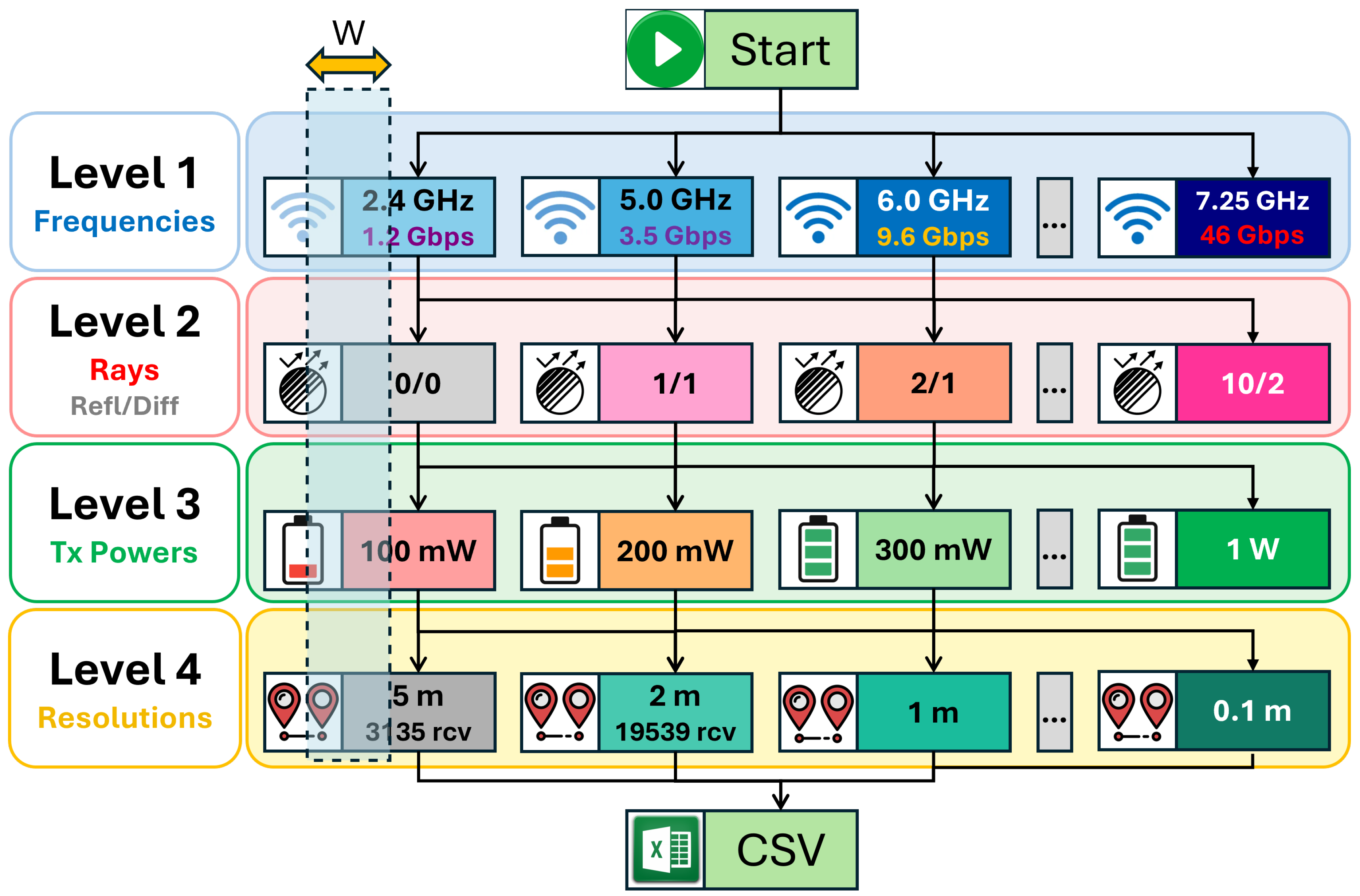
The configuration space is organized into four levels:
- Level 1 – Frequencies: We simulate signal propagation for wireless frequencies including 2.4 GHz, 5.0 GHz, and 6.0 GHz. Each frequency corresponds to a nominal modulation capacity (e.g., 1.2 Gbps for 2.4 GHz, 9.6 Gbps for 6.0 GHz). Additional higher-frequency bands such as 7.25 GHz may also be considered in extended studies.
- Level 2 – Ray Configurations: MATLAB’s ray-tracing engine supports a maximum of 10 reflections and 2 diffractions. However, due to the significant increase in computational time when simulating two diffractions, we limited this study to a maximum of 10 reflections and 1 diffraction. Each configuration is represented as R/D, denoting the number of allowed reflections (R) and diffractions (D), e.g., 0/0, 1/0, ..., 10/0, and 0/1, 1/1, ..., 10/1.
- Level 3 – Transmit Power Levels: For each ray configuration, we simulate four transmit power levels: 0.1 W, 0.2 W, 0.3 W, and 1.0 W. These settings allow us to investigate signal propagation under various transmission conditions.
- Level 4 – Spatial Resolutions: Receiver positions are sampled with spatial resolutions of 5 m, 2 m, 1 m, and 0.1 m. The number of receivers increases accordingly, from 135 receivers at 5 m spacing to over 19,000 at 2 m resolution. The 0.1 m setting was primarily used in isolated test cases due to its high computational cost.
To manage the large number of simulations, we distributed the workload across four parallel servers. Each server executed 3, 6, 9, or 12 MATLAB instances concurrently, depending on resource availability. Each instance processed up to 3,210 receiver positions per configuration, iterating through all selected combinations of frequency, propagation complexity, transmit power, and spatial resolution.
Simulation outputs were saved as structured CSV files, one per configuration, for reproducibility and downstream analysis. This hierarchical, parallelized setup enabled wide coverage of the parameter space within practical hardware and software limits.
Appendix B Dataset Description and Feature Definitions
This appendix provides a detailed description of the dataset generated and used in this study. The dataset was obtained through extensive MATLAB-based ray-tracing simulations conducted over a large-scale urban campus environment and serves as the foundation for all machine learning experiments presented in the paper.
Each row in the dataset corresponds to a single transmitter–receiver (Tx–Rx) link evaluated under a specific combination of frequency band, transmit power, ray-tracing configuration, and receiver location. The dataset is designed to preserve both the physical interpretability of wireless propagation and the statistical richness required for data-driven modeling, neural architecture search, and digital twin integration.
Appendix B.1. Dataset Design Philosophy
The dataset follows three core design principles:
- Physics-preserving: All features originate directly from deterministic ray-tracing outputs or geometric calculations, ensuring alignment with electromagnetic propagation theory.
- Model-agnostic: No handcrafted feature engineering or dimensionality reduction was applied prior to learning, allowing different model families (tree-based, neural, transformer-based) to exploit the data according to their inductive biases.
- Scalable and extensible: The feature schema supports future extensions such as adaptive antennas, beamforming, mobility, and dynamic environmental changes.
This design enables the dataset to function not only as a training corpus, but also as a reusable asset for future studies on network optimization and AI-driven radio planning.
Appendix B.2. Feature Categories
For interpretability and clarity, the dataset columns can be grouped into the following categories:
- Identifiers and metadata, used for indexing, bookkeeping, and traceability.
- Transmitter and receiver geometry, describing spatial placement, distance, and relative orientation.
- Radio configuration parameters, defining frequency, transmit power, and antenna height.
- Ray-tracing interaction statistics, capturing multipath complexity through reflections and diffractions.
- Target variables, representing received signal strength.
- Auxiliary performance metrics, such as simulation runtime.
This categorization mirrors the structure of the MATLAB simulation pipeline and facilitates direct interpretation of learned feature importance and correlations.
Appendix B.3. Complete Feature List
Table A1 provides the complete list of dataset columns, along with concise descriptions and measurement units.
Appendix B.4. Target Variables
The supervised learning targets in this study are rssi1 and rssi2, which represent two independently computed received power estimates provided by MATLAB’s propagation framework. Unless explicitly stated otherwise, rssi1 is used as the primary regression target due to its numerical stability and consistent behavior across simulation configurations. Both targets are retained to support future multi-output learning scenarios and uncertainty analysis.

Table A1.
Complete list of dataset columns and descriptions used in this study.
| # | Column Name | Description |
|---|---|---|
| 1 | receiver_index | Unique identifier for each receiver position within the circular grid layout |
| 2 | tx_latitude | Latitude of the transmitter in decimal degrees [°] |
| 3 | tx_longitude | Longitude of the transmitter in decimal degrees [°] |
| 4 | tx_frequency | Transmission frequency [Hz], spanning 2.4, 5, and 6 GHz bands |
| 5 | tx_power | Transmit power [W] (100–1000 mW) |
| 6 | tx_antenna_height | Transmitter antenna height above ground [m] |
| 7 | tx_elevation | Terrain elevation at transmitter site [m] |
| 8 | rx_latitude | Receiver latitude in decimal degrees [°] |
| 9 | rx_longitude | Receiver longitude in decimal degrees [°] |
| 10 | rx_antenna_height | Receiver antenna height above ground [m] |
| 11 | rx_elevation | Terrain elevation at receiver location [m] |
| 12 | rx_sensitivity | Receiver sensitivity threshold [dBm] |
| 13 | distance_tx_rx | Tx–Rx separation distance [m] |
| 14 | azimuth_angle | Horizontal bearing from transmitter to receiver [°] |
| 15 | elevation_angle | Vertical angle between transmitter and receiver [°] |
| 16 | rt_reflections | Maximum number of reflections allowed by the simulation configuration |
| 17 | rt_diffractions | Maximum number of diffractions allowed by the simulation configuration |
| 18 | nb_rays | Total number of rays launched by the SBR engine |
| 19 | nb_interactions | Total number of ray interactions (reflections + diffractions) |
| 20 | len_interactions | Number of interaction hops along the dominant ray path |
| 21 | ray_max_nb_reflections | Maximum reflections encountered by any single ray |
| 22 | ray_max_nb_diffractions | Maximum diffractions encountered by any single ray |
| 23 | total_nb_reflections | Total reflection events aggregated across all rays |
| 24 | total_nb_diffractions | Total diffraction events aggregated across all rays |
| 25 | rssi1 | Received Signal Strength Indicator (RSSI) [dBm] |
| 26 | rssi2 | Received Signal Strength Indicator (RSSI), heavy rain [dBm] |
| 27 | elapsed_time | Simulation runtime per receiver position [ms] |
Appendix B.5. Feature Usage in Machine Learning
All numerical features, excluding identifiers and runtime metadata, are retained during training. Columns such as receiver_index and elapsed_time are excluded from the learning process but preserved for traceability, debugging, and computational analysis.
No features were removed solely based on correlation strength. This decision reflects the adoption of transformer-based architectures, which are capable of learning complex, nonlinear interactions between correlated inputs without manual feature pruning. As a result, the dataset maintains its full descriptive richness while enabling the model to learn both dominant and subtle propagation effects.
Appendix B.6. Forward Compatibility
Although the current dataset uses a fixed, center-fed dipole antenna at a static transmitter location, the feature schema is intentionally forward-compatible. Angular features, interaction counts, and geometric descriptors are expected to play a significantly larger role in future extensions involving directional antennas, beamforming, mobility, and adaptive transmission strategies within a digital twin framework.
This makes the dataset suitable not only for the experiments presented in this paper, but also for continued research on AI-native wireless network planning and optimization.
Appendix C Server Infrastructure and Parallel Execution Strategy
To manage the large-scale parameter space of the ray-tracing simulations, we deployed a parallel execution framework across four dedicated simulation servers. Each server was equipped with multi-core CPUs capable of running several independent MATLAB R2024b instances simultaneously. Every instance executed a distinct configuration from the hierarchical space detailed in Appendix A.
The configuration distribution was performed manually by partitioning sets of receiver positions and ray-tracing parameters, including combinations of frequency (2.4 GHz, 5.0 GHz, 6.0 GHz), transmit power levels, and propagation complexity (reflections/diffractions). Each MATLAB process independently loaded a receiver grid and completed a batch of simulations, writing outputs to structured CSV files.
- Platinum Server: Lenovo ThinkStation P720, powered by an Intel Xeon Platinum 8160 CPU with 24 cores. It was configured to run 12 parallel MATLAB instances at 100% CPU utilization. This high-end workstation was the most productive node, suitable for long-duration, high-resolution runs.
- Gold Server: Lenovo ThinkStation P720 with Intel Xeon Gold 6138 (20 cores). Typically ran 3–12 MATLAB instances concurrently.
- Other Nodes: Two additional servers with similar Intel Xeon CPUs (Silver-series), configured for 3–6 MATLAB windows depending on core count and thermal limits.
Figure C1.
Hardware configuration of the primary ray-tracing and machine learning simulation servers.
Figure C1.
Hardware configuration of the primary ray-tracing and machine learning simulation servers.
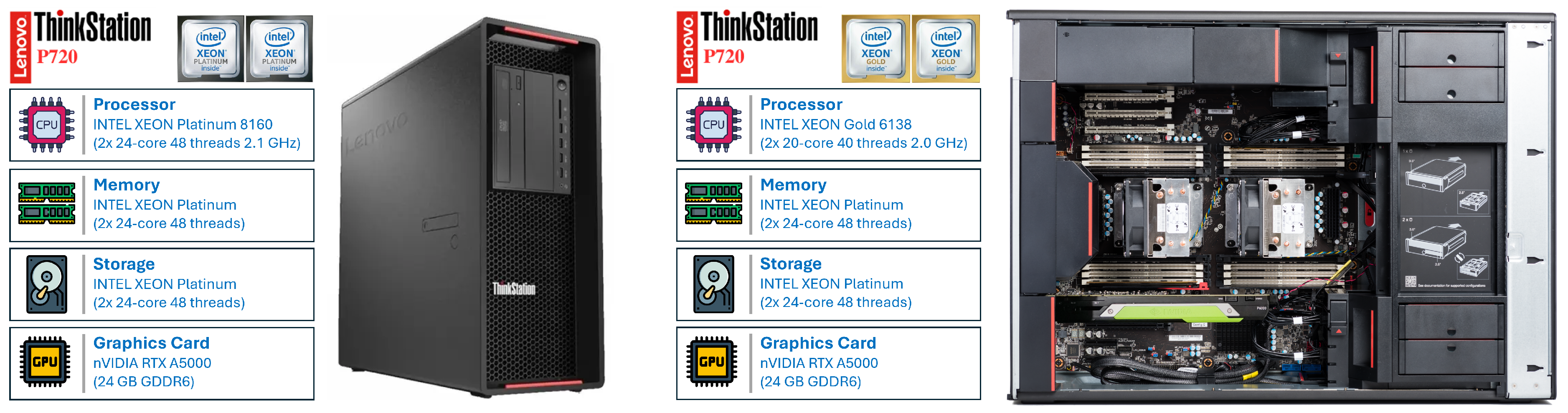
Each MATLAB window acted independently, ensuring robustness and parallelism without shared memory dependencies. Simulation logs were saved per instance, and failures could be recovered by restarting individual windows. This parallel strategy enabled the evaluation of thousands of configurations in a fraction of the time required for sequential execution.
Figure C2 shows the Gold server running 12 MATLAB R2024b instances in parallel, actively processing spatially distributed receiver points across the defined simulation region.
Appendix C.1. CPU Classes and Server Roles
The simulation workloads in this study were executed across two primary server types, each equipped with different classes of Intel Xeon CPUs. The primary node, referred to as the Platinum Server, is a Lenovo ThinkStation P720 configured with two Intel Xeon Platinum 8160 processors (24 cores, 48 threads each). This dual-socket configuration offered 96 logical threads, allowing for highly parallelized MATLAB execution across up to 12 simultaneous instances with sustained performance.
In contrast, the secondary node, referred to as the Gold Server, is a Lenovo ThinkStation P720 equipped with a single Intel Xeon Gold 6138 CPU (20 cores, 40 threads). Although still capable of multi-instance execution, its total compute capacity was comparable to Platinum, supporting between 3 and 12 parallel MATLAB instances depending on ray-tracing configuration (the higher the number of reflections and diffractions used, the lower the number of parallel MATLAB instances used).
Figure C2.
Screenshot of 12 parallel MATLAB R2024b instances running on the Lenovo ThinkStation P720, powered by 2 x Intel Xeon Gold 6138 CPUs. Each instance executes a distinct ray-tracing configuration, achieving full CPU utilization across all logical cores.
Figure C2.
Screenshot of 12 parallel MATLAB R2024b instances running on the Lenovo ThinkStation P720, powered by 2 x Intel Xeon Gold 6138 CPUs. Each instance executes a distinct ray-tracing configuration, achieving full CPU utilization across all logical cores.
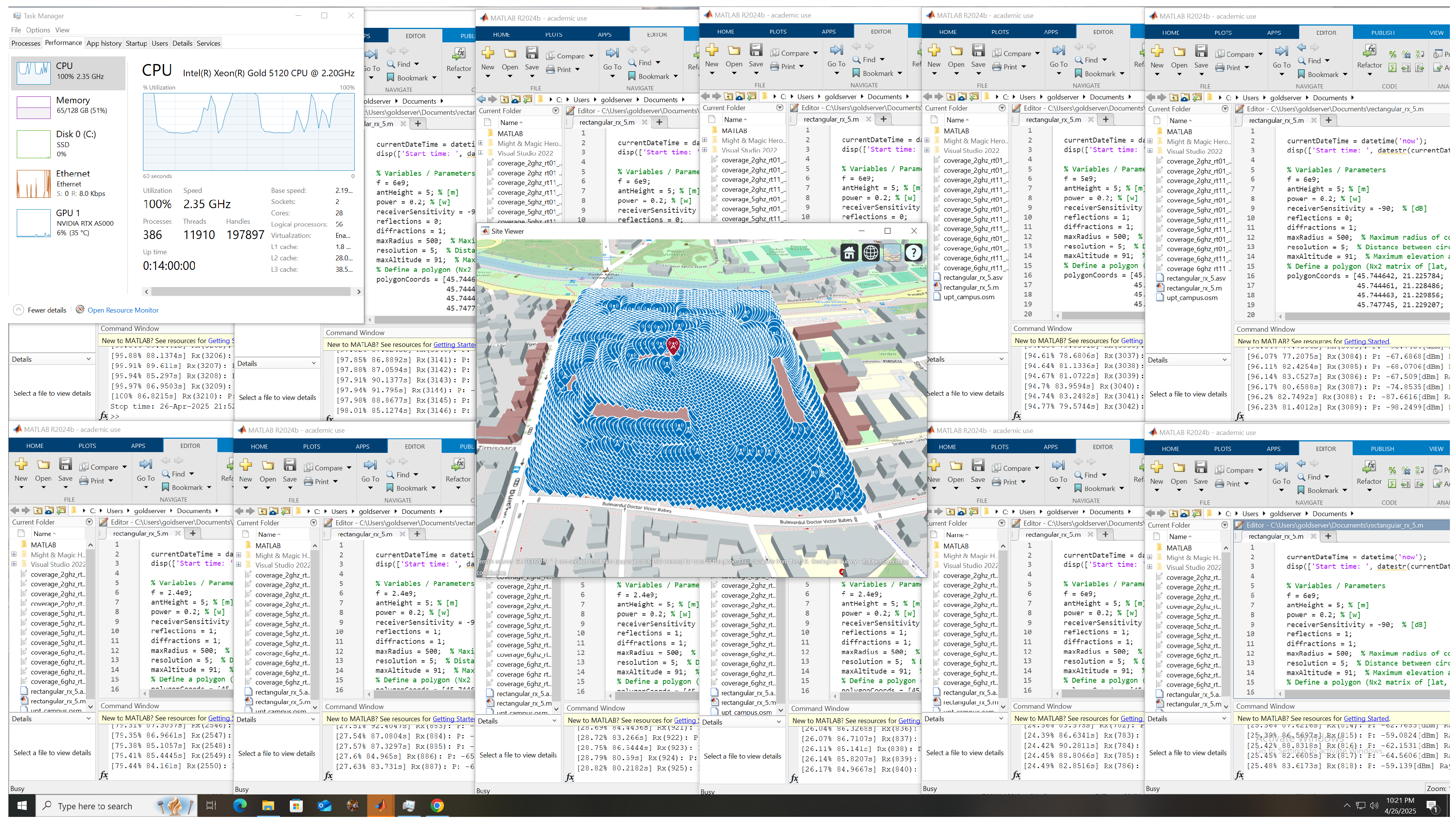
Figure C3 provides an architectural overview of Intel Xeon Scalable processor tiers. It highlights the relative positioning of the Gold and Silver series CPUs used in this study, emphasizing the intended segmentation of compute performance and scalability in server-grade hardware.
Figure C3.
Reference diagram illustrating Intel Xeon Scalable processor tiers. This architecture overview highlights the positioning of Platinum- and Gold-series CPUs used in this study. One of our primary simulation servers (Platinum Server) was equipped with two Intel Xeon Platinum CPUs (8160, 24-core, 2.1 GHz, 33 MB cache), while the secondary server (Gold Server) used an Intel Xeon Gold-class CPU (6138, 20-core 2.00 GHz, 27.5 MB cache). This distinction reflects a performance hierarchy in compute capacity and parallel instance throughput.
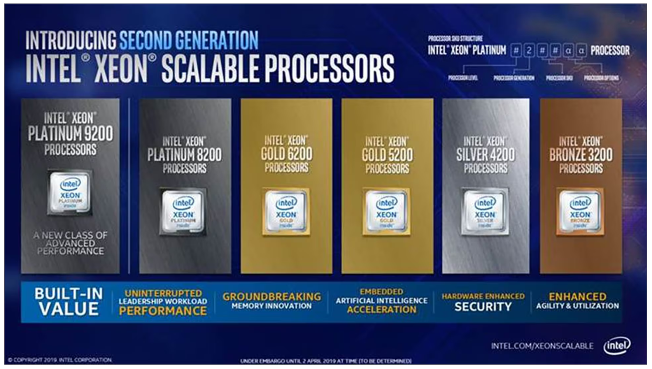
Intel’s second-generation Xeon Scalable processors are organized into performance tiers designed for various levels of compute intensity and scalability, as illustrated in Figure C3. The processors range from Bronze for entry-level workloads to Platinum for mission-critical multi-socket applications.
The simulations in this study were executed on 2 servers, one equipped with 2 Intel Xeon Platinum 8160 CPUs which belong to the Platinum 8200 series, another one equipped with 2 Intel Xeon Gold 6138 CPUs which belong to the Platinum 6200 series. These processors support Intel® Deep Learning Boost (DL Boost) via Vector Neural Network Instructions (VNNI), providing native acceleration for deep learning inference tasks. This enables moderate AI workloads, such as signal classification or anomaly detection, to be executed on the CPU without requiring a discrete GPU, reducing latency and power consumption.
While the focus of this study was ray-tracing simulation, the choice of hardware positions the system for future integration of AI-assisted modeling, hybrid simulation-learning workflows, or adaptive signal processing pipelines that benefit from on-chip AI capabilities.
References
- Szott, S.; Kosek-Szott, K.; et al. Wi-Fi meets ML: A survey on improving IEEE 802.11 performance with machine learning. arXiv 2021, arXiv:2109.04786. [Google Scholar] [CrossRef]
- Alabi, M. The Evolution of Wi-Fi Standards: From Wi-Fi 6 to Wi-Fi 7. ResearchGate Preprint 2023. Accessed: 2024-05-13. [Google Scholar]
- Naik, G.; Park, J.M.; Ashdown, J.; Lehr, W. Next Generation Wi-Fi and 5G NR-U in the 6 GHz Bands: Opportunities & Challenges. arXiv 2020, arXiv:cs.NI/2006.16534. [Google Scholar]
- Andrews, J.G.; Buzzi, S.; Choi, W.; Hanly, S.V.; Lozano, A.; Soong, A.C.K.; Zhang, J.C. What Will 5G Be? IEEE Journal on Selected Areas in Communications 2014, 32, 1065–1082. [Google Scholar] [CrossRef]
- Park, J.; Samarakoon, S.; Bennis, M.; Debbah, M. Wireless Network Intelligence at the Edge. arXiv 2019, arXiv:cs.IT/1812.02858. [Google Scholar] [CrossRef]
- Fuschini, F.; Vitucci, E.M.; Barbiroli, M.; Falciasecca, G.; Degli-Esposti, V. Ray tracing propagation modeling for future small-cell and indoor applications: A review of current techniques. Radio Science 2015, 50, 469–485. [Google Scholar] [CrossRef]
- Yun, Z.; Iskander, M.F. Ray Tracing for Radio Propagation Modeling: Principles and Applications. IEEE Access 2015, 3, 1089–1100. [Google Scholar] [CrossRef]
- Amro, M.; Landolsi, A.; Zummo, S.; Grieger, M.; Danneberg, M.; Fettweis, G. Ray-tracing wireless channel modeling and verification in Coordinated Multi-Point systems. In Proceedings of the 2014 12th International Symposium on Modeling and Optimization in Mobile, Ad Hoc, and Wireless Networks (WiOpt), 2014; pp. 16–21. [Google Scholar]
- Grieves, M.; Vickers, J. Digital Twin: Mitigating Unpredictable, Undesirable Emergent Behavior in Complex Systems. 2017; 85–113. [Google Scholar]
- Tao, F.; Cheng, J.; Qi, Q.; Zhang, M.; Zhang, H.; Sui, F. Digital twin-driven product design, manufacturing and service with big data. The International Journal of Advanced Manufacturing Technology 2018, 94. [Google Scholar] [CrossRef]
- Choi, H.; Oh, J.; Chung, J.; Alexandropoulos, G.C.; Choi, J. WiThRay: A Versatile Ray-Tracing Simulator for Smart Wireless Environments. IEEE Access 2023, 11, 56822–56845. [Google Scholar] [CrossRef]
- Chen, Z.; Xu, X.; Zhang, P. Radio Transformer Networks: Attention-Based End-to-End Learning for Wireless Channel Modeling. IEEE Transactions on Wireless Communications 2022, 21, 8360–8374. [Google Scholar]
- Xu, B.; Li, Y.; Jiang, C.; Wang, X. Neural Radio Map: Transformer-Based Channel Prediction. IEEE Access 2023, 11, 119204–119217. [Google Scholar]
- Huang, X.; Khetan, A.; Cvitkovic, M.; Karnin, Z. TabTransformer: Tabular Data Modeling Using Contextual Embeddings. In Proceedings of the Proceedings of the AAAI Conference on Artificial Intelligence, 2021; pp. 5962–5970. [Google Scholar]
- Gorishniy, Y.; Rubachev, I.; Khrulkov, V.; Babenko, A. Revisiting Deep Learning Models for Tabular Data. In Proceedings of the Advances in Neural Information Processing Systems (NeurIPS), 2021. [Google Scholar]
- Deng, C.; Fang, X.; et al. IEEE 802.11be: Wi-Fi 7—New challenges and opportunities. arXiv 2020, arXiv:2007.13401. [Google Scholar] [CrossRef]
- López-Pérez, D.; Garcia-Rodriguez, A.; et al. IEEE 802.11be extremely high throughput: The next generation of Wi-Fi technology beyond 802.11ax. arXiv 2019, arXiv:1902.04320. [Google Scholar] [CrossRef]
- Ning, J.; Deng, J.; Li, Y.; Zhao, C.; Liu, J.; Yang, S.; Wang, Y.; Huang, J.; Wang, C.X. Ray-Tracing Channel Modeling for LEO Satellite-to-Ground Communication Systems. In Proceedings of the 2024 IEEE/CIC International Conference on Communications in China (ICCC), 2024; pp. 1169–1174. [Google Scholar]
- Islam, R.; Mahbub, F.; Akash, S.; Al-Nahiun, S.A.K. Design of a Half-Wave Dipole Antenna for Wi-Fi & WLAN System using ISM Band. 04 2021; 1–4. [Google Scholar]
- Tareq, M.; Alam, D.; Islam, M.; Ahmed, R. Simple Half-Wave Dipole Antenna Analysis for Wireless Applications by CST Microwave Studio. International Journal of Computer Applications 2014, 94, 975–8887. [Google Scholar] [CrossRef]
| 1 | In our file naming, RT101 denotes the specific ray-tracing setup used in this experiment, in this particular case 10 reflections and 1 diffraction. |
| 2 | In this paper, offline refers to computationally intensive, non-real-time MATLAB ray-tracing simulations executed prior to deployment, whereas online denotes the low-latency inference of trained machine-learning models for new or unseen scenarios. |
Figure 1.
Politehnica Timișoara University Campus with AP on top of Mechatronics (building O).
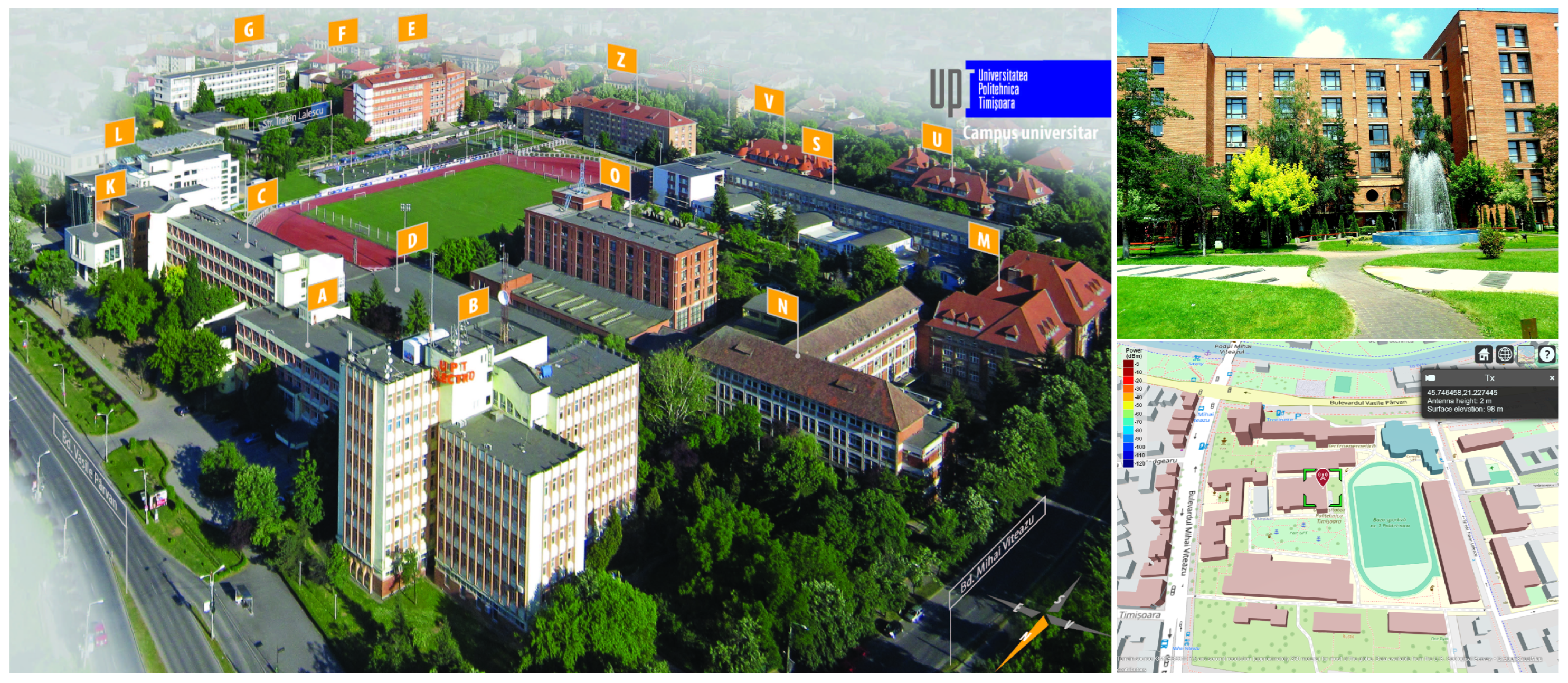
Figure 2.
Timeline of IEEE 802.11 standard evolution from 1997 to 2024, highlighting key technical milestones and application trends from 802.11 (Wi-Fi 1) to 802.11be (Wi-Fi 7). Source: Ruijie Networks.
Figure 2.
Timeline of IEEE 802.11 standard evolution from 1997 to 2024, highlighting key technical milestones and application trends from 802.11 (Wi-Fi 1) to 802.11be (Wi-Fi 7). Source: Ruijie Networks.
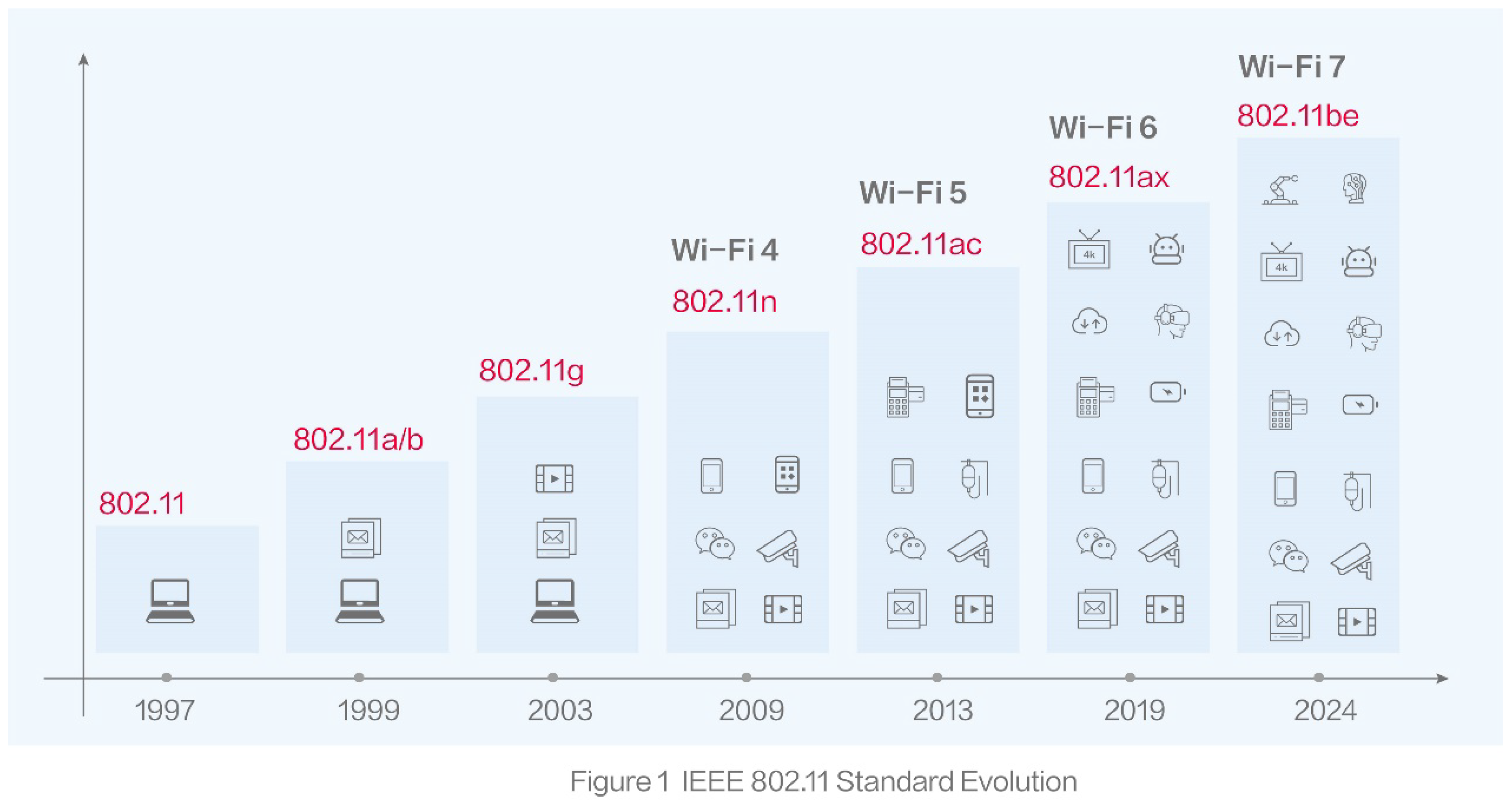
Figure 3.
Constellation diagrams illustrating modulation complexity in Wi-Fi standards. The number of distinct symbols increases exponentially from 64-QAM (Wi-Fi 4) to 4096-QAM (Wi-Fi 7), highlighting increased data rates and signal precision requirements. Source: Alta Inc.
Figure 3.
Constellation diagrams illustrating modulation complexity in Wi-Fi standards. The number of distinct symbols increases exponentially from 64-QAM (Wi-Fi 4) to 4096-QAM (Wi-Fi 7), highlighting increased data rates and signal precision requirements. Source: Alta Inc.
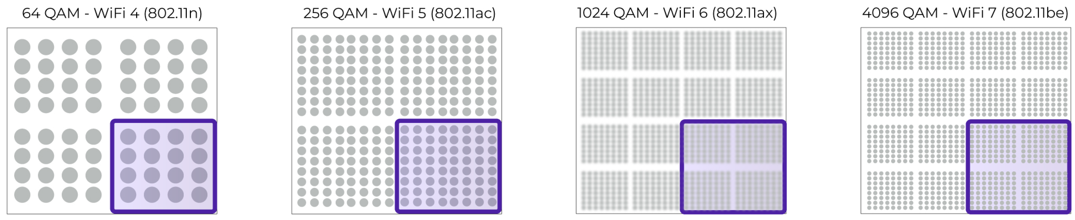
Figure 4.
Visualization of QAM modulation. Left: Time-domain example of mapping 3-bit symbols at a baud rate of 8 symbols/s for a bit rate of 24 bps. Right: Constellation diagrams for 4-QAM, 8-QAM, and 16-QAM, showing the increased complexity and tighter spacing of symbols with higher-order modulation.
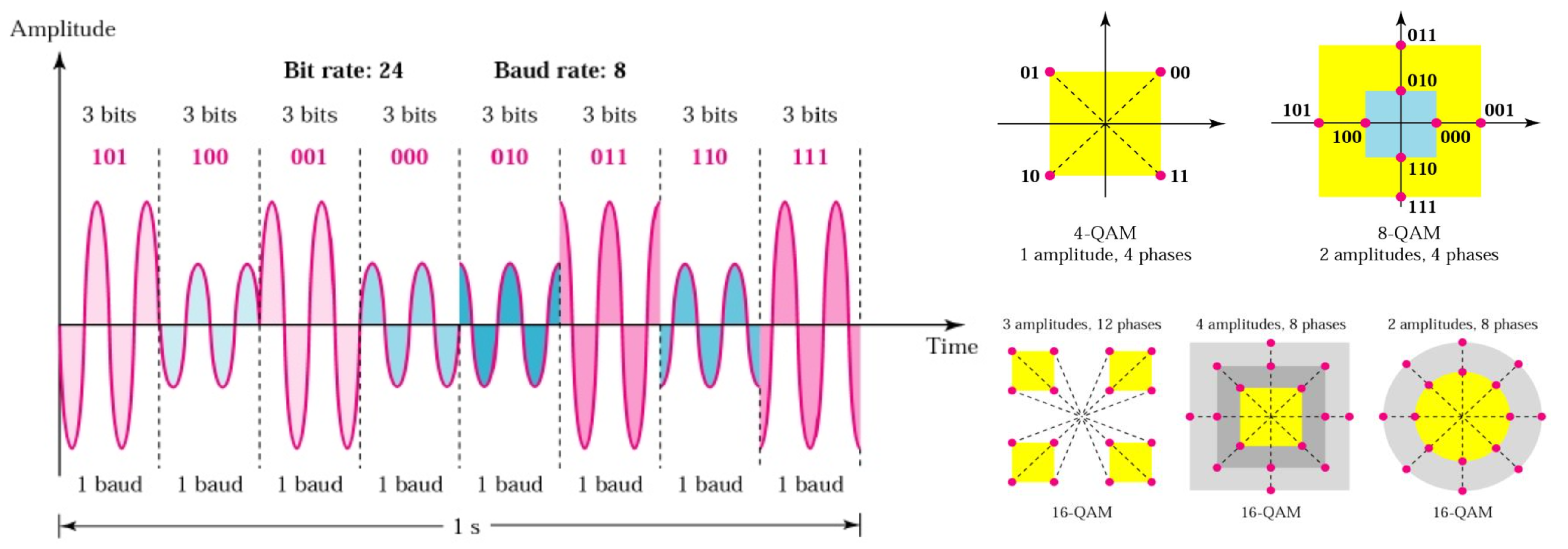
Figure 5.
Comparison of channel bandwidth and data capacity across Wi-Fi generations. Wi-Fi 7 enables 320 MHz channels and up to 46 Gbps throughput. Earlier versions like Wi-Fi 6 and 5 are limited by narrower bandwidths and more congested bands. Sources: ASUS, SoundDD.
Figure 5.
Comparison of channel bandwidth and data capacity across Wi-Fi generations. Wi-Fi 7 enables 320 MHz channels and up to 46 Gbps throughput. Earlier versions like Wi-Fi 6 and 5 are limited by narrower bandwidths and more congested bands. Sources: ASUS, SoundDD.
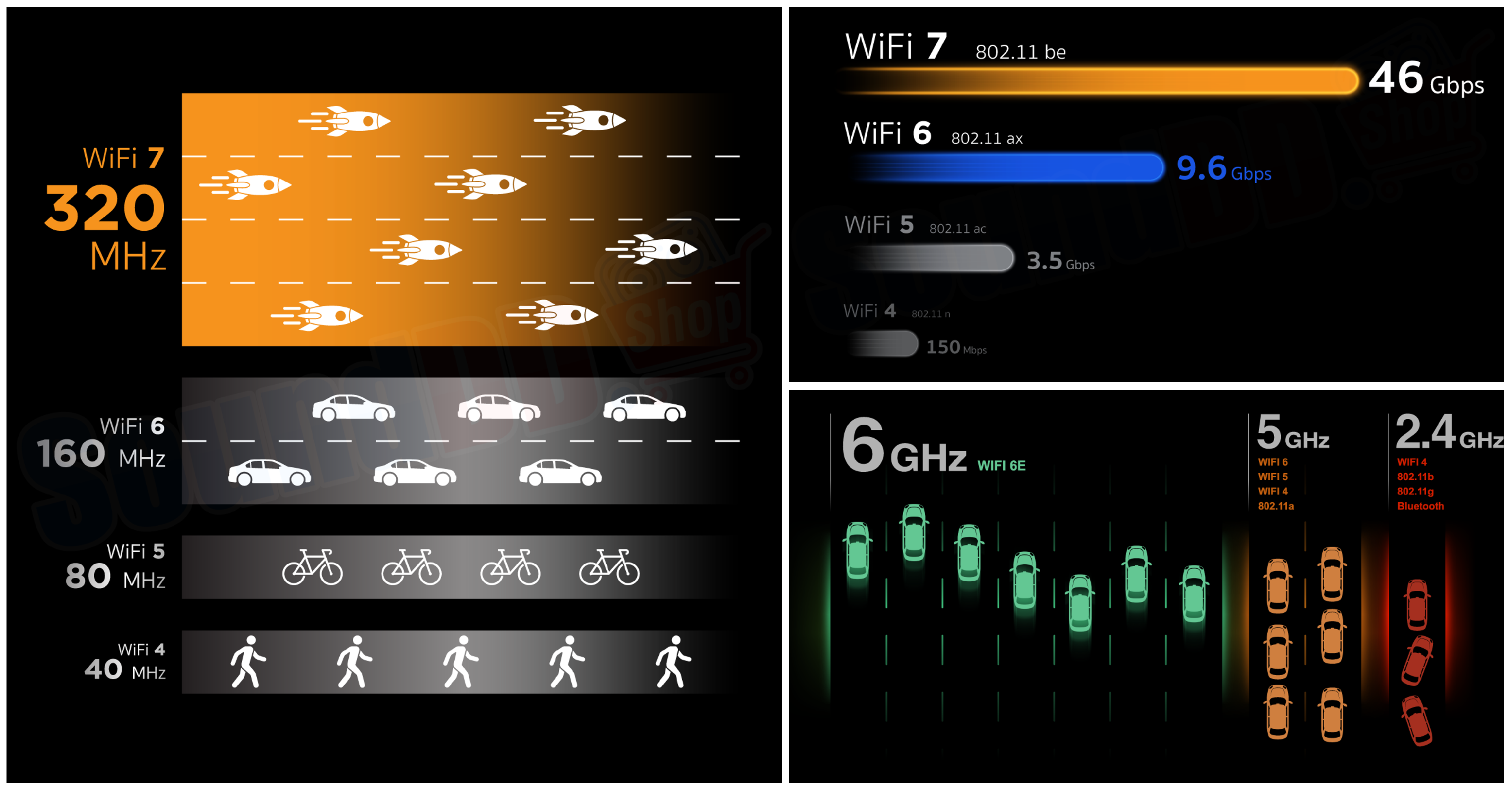
Figure 6.
Channel allocation and interference mechanisms in the 2.4 GHz Wi-Fi band for 20–22 MHz channels. From top to bottom, the figure illustrates adjacent-channel interference, extensive channel overlap caused by 5 MHz channel spacing, and co-channel interference when multiple access points operate on the same channel. Due to the limited available spectrum, only a small number of non-overlapping channels can be used simultaneously, which significantly constrains capacity and spatial reuse in dense deployments. Images adapted from Ekahau.
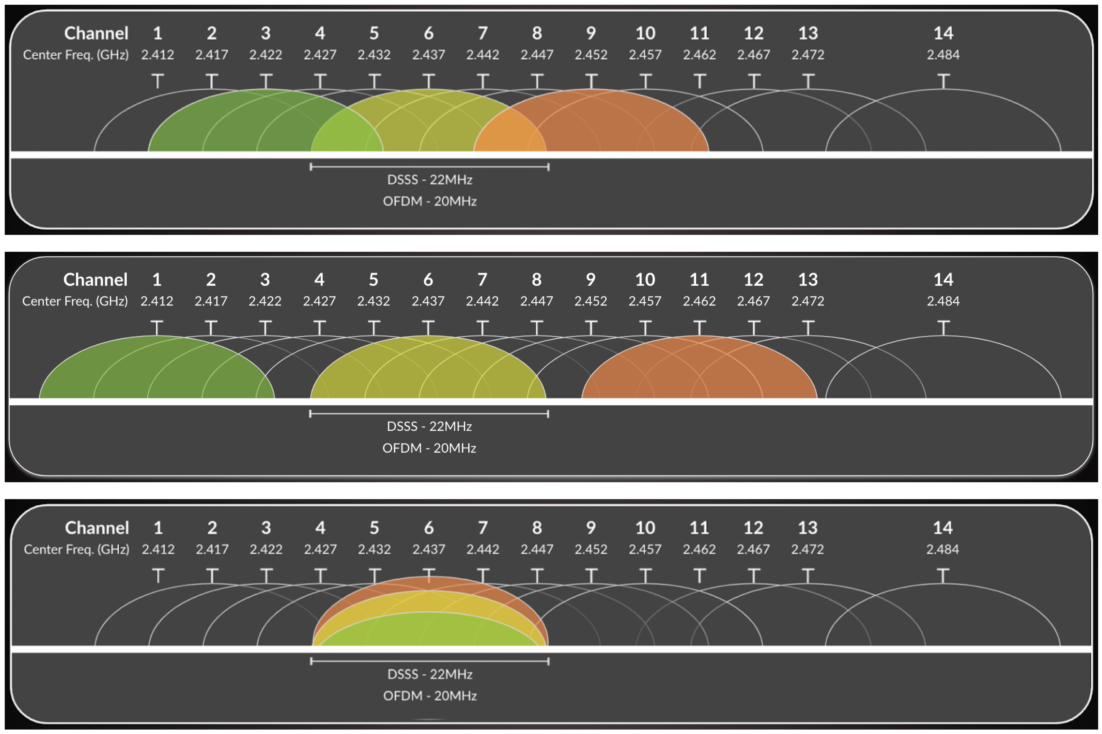
Figure 7.
Overview of the 5 GHz Wi-Fi spectrum illustrating channel allocation across the U-NII sub-bands, including DFS-regulated frequencies and available non-overlapping channels for 20 MHz and 40 MHz operation. The figure highlights the increased spectral availability compared to the 2.4 GHz band, as well as the practical constraints introduced by Dynamic Frequency Selection in certain portions of the spectrum. Image adapted from publicly available sources.
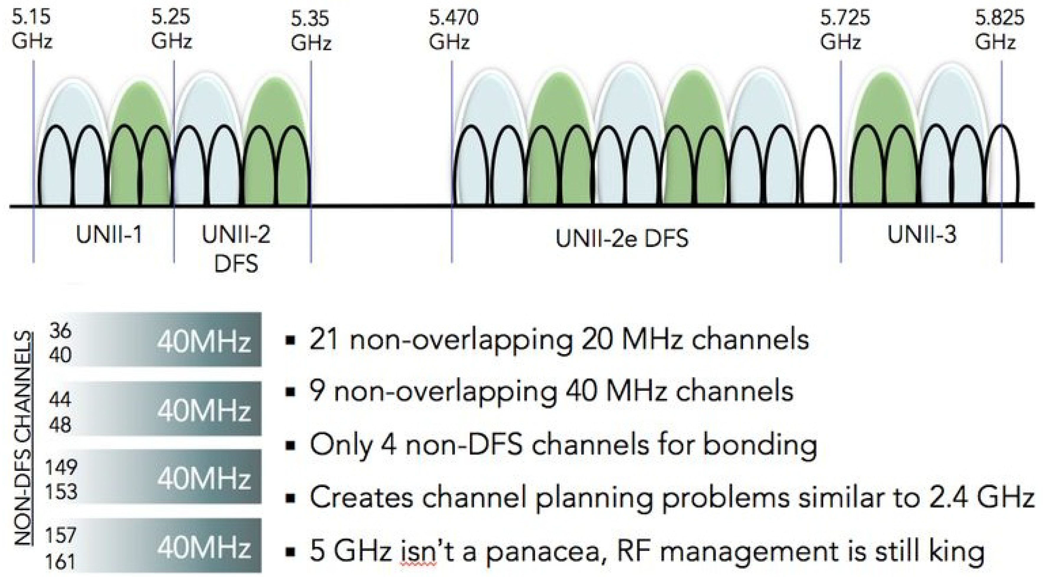
Figure 8.
Channel allocation of the 6 GHz Wi-Fi band illustrating 20, 40, 80, 160, and 320 MHz channel groupings across the U-NII-5, U-NII-6, U-NII-7, and U-NII-8 sub-bands. The figure highlights actual channel numbers, center frequencies, and regulatory distinctions between low-power indoor (LPI) and standard-power access point operation with automated frequency coordination (AFC). The expanded contiguous spectrum enables ultra-wide 320 MHz channels introduced with IEEE 802.11be (Wi-Fi 7), supporting extremely high-throughput outdoor and campus-scale deployments. Image adapted from publicly available regulatory and technical sources.
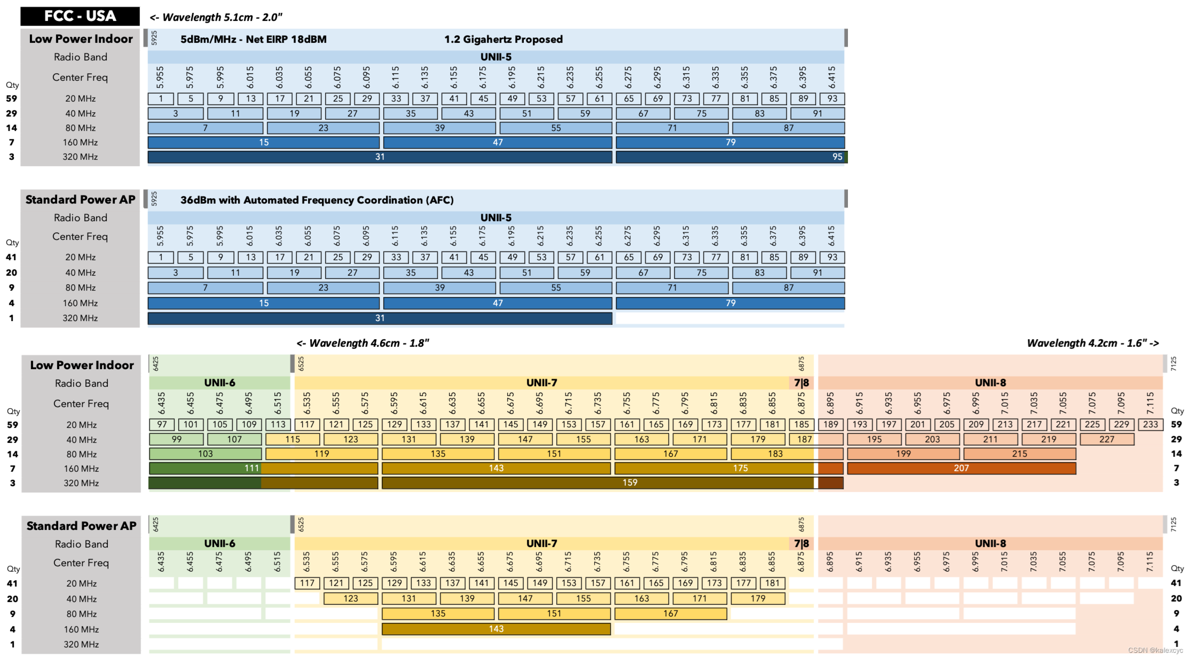
Figure 9.
Example of deterministic ray-tracing visualization in MATLAB showing multiple propagation paths between a transmitter and a receiver in a three-dimensional urban environment. Each ray is characterized by its number of reflections and diffractions, interaction materials, path length, phase change, and angular properties. Color coding indicates path loss (dB), highlighting the attenuation differences between LoS, reflected, and diffracted paths (source: Mathworks website).
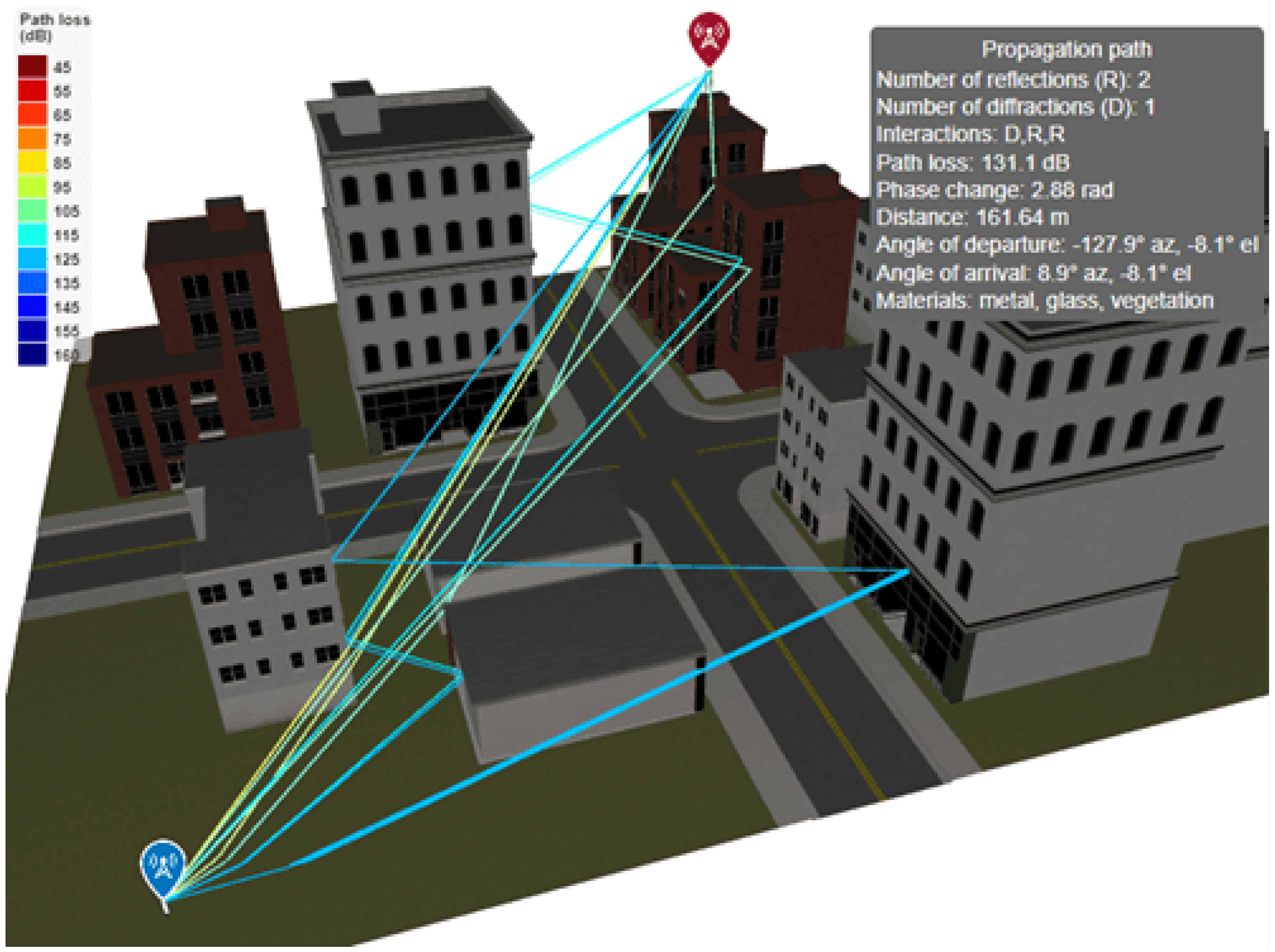
Figure 10.
Reflection–diffraction configuration matrix used in the MATLAB coverage map simulation. Each R/D cell corresponds to a unique propagation model setup that can be repeated across frequencies (2.4, 5, and 6 GHz) and transmit power levels (100, 200, 500, and 1000 mW).
Figure 10.
Reflection–diffraction configuration matrix used in the MATLAB coverage map simulation. Each R/D cell corresponds to a unique propagation model setup that can be repeated across frequencies (2.4, 5, and 6 GHz) and transmit power levels (100, 200, 500, and 1000 mW).
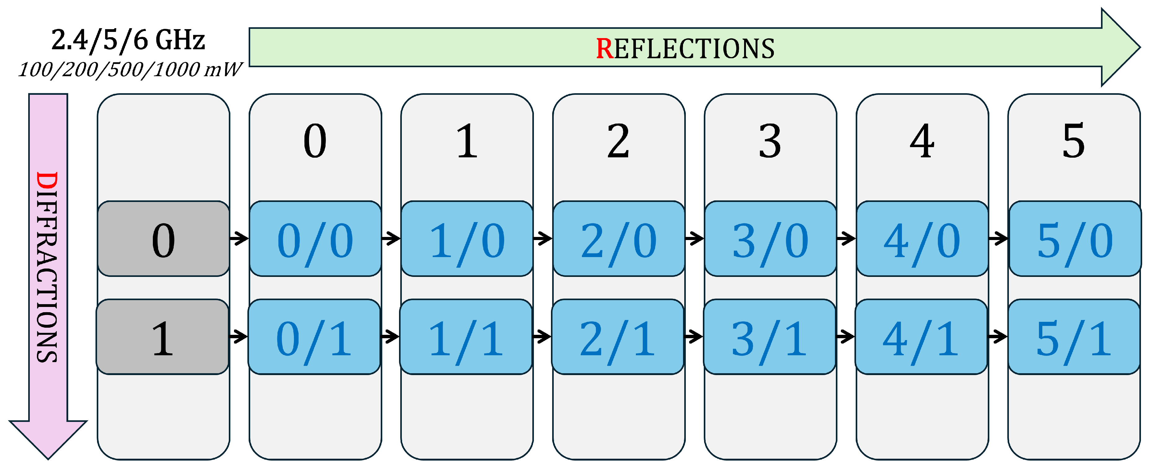
Figure 11.
3D radio coverage map generated in MATLAB’s siteviewer environment using the ray-tracing model (MaxNumReflections = 1, MaxNumDiffractions = 1) at 2.4 GHz, 0.1 W transmit power. The transmitter is positioned on top of the Mechatronics (building O) of the Politehnica University of Timișoara campus. The color scale indicates received power (dBm).
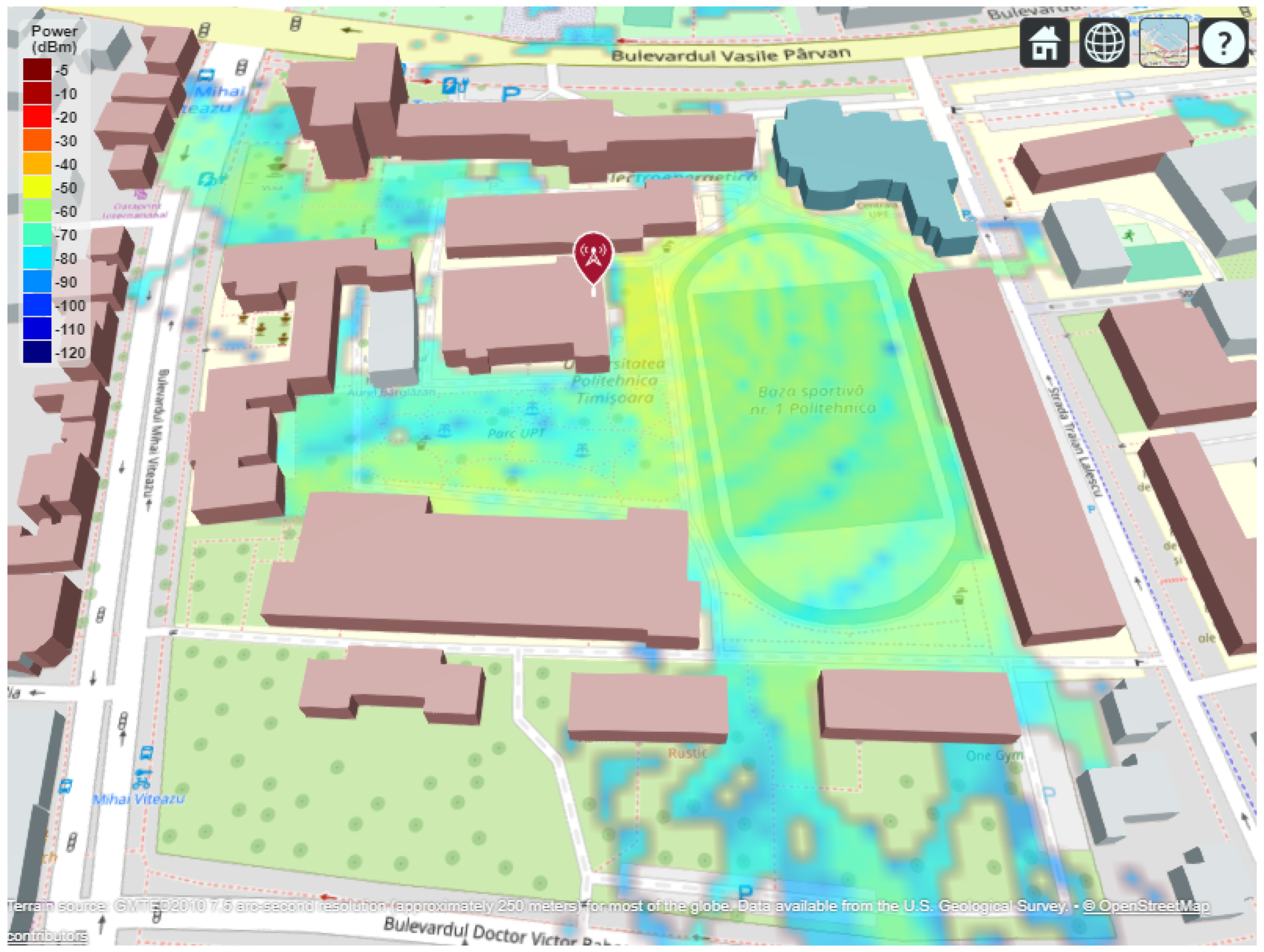
Figure 12.
Half-wave dipole antenna models and radiation behavior at 2.4 GHz, 5.0 GHz, and 6.0 GHz. Left: azimuthal directivity cut (near-omnidirectional in the horizontal plane). Center: 3D dipole geometry generated by MATLAB (design(dipole,f)). Right: 3D directivity distribution showing the expected toroidal pattern with nulls along the dipole axis.
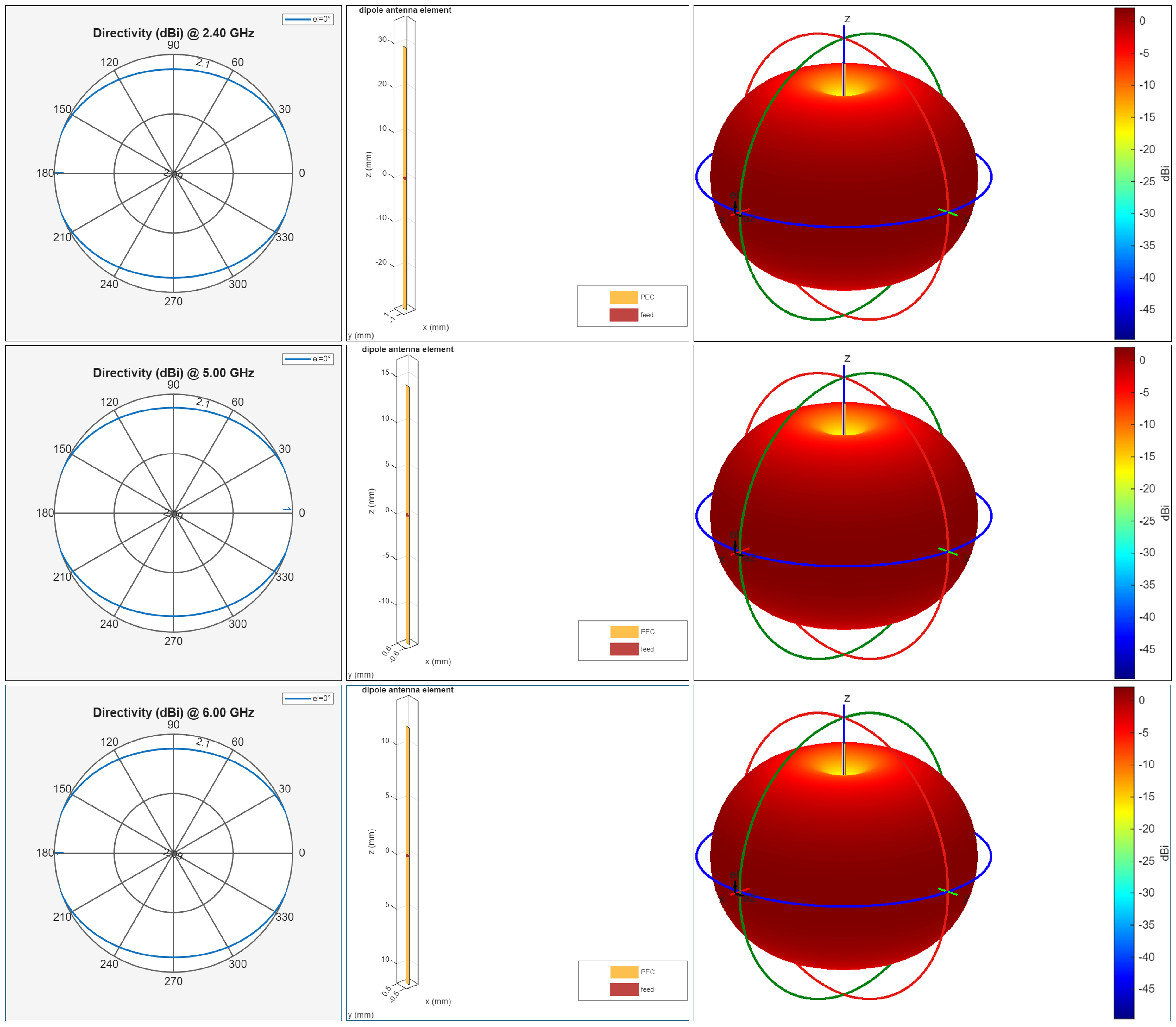
Figure 13.
Circular receiver array MATLAB visualization around a central transmitter (Electro building B, Polytechnic University Timișoara Campus). The receivers are evenly distributed along a circular perimeter, with coverage visualization shown both in 2D (left) and 3D (right).
Figure 13.
Circular receiver array MATLAB visualization around a central transmitter (Electro building B, Polytechnic University Timișoara Campus). The receivers are evenly distributed along a circular perimeter, with coverage visualization shown both in 2D (left) and 3D (right).
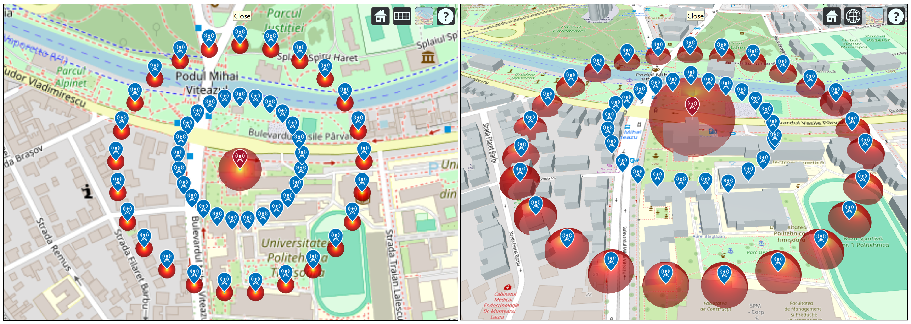
Figure 14.
Receiver site generation using a resolution-driven concentric-circle strategy. Multiple circles are placed around the transmitter with radial spacing , while the number of receivers per circle is computed from the circle circumference to maintain approximately meters spacing along the arc. Receivers are retained only if they fall inside the user-defined polygon footprint (campus area) and satisfy an optional elevation threshold; the inset emphasizes the dense sampling near the transmitter.
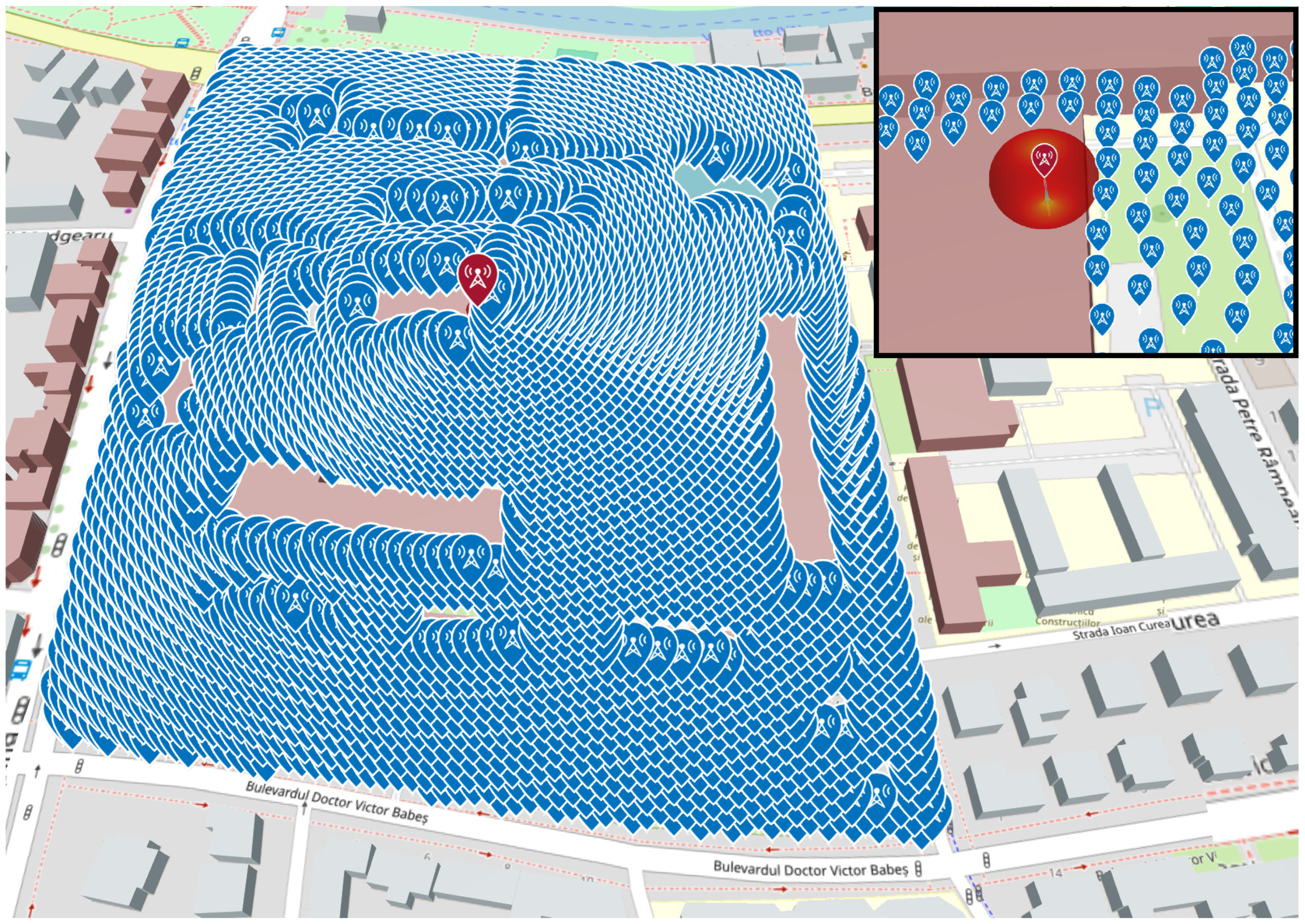
Figure 15.
Illustration of the decomposition of variance in linear regression. The total sum of squares (SST) measures the variance of the observed data around the mean, the regression sum of squares (SSR) represents the variance explained by the model, and the sum of squared errors (SSE) captures the residual error. The coefficient of determination quantifies the ratio of explained variance to total variance (source: vitaflux.com).
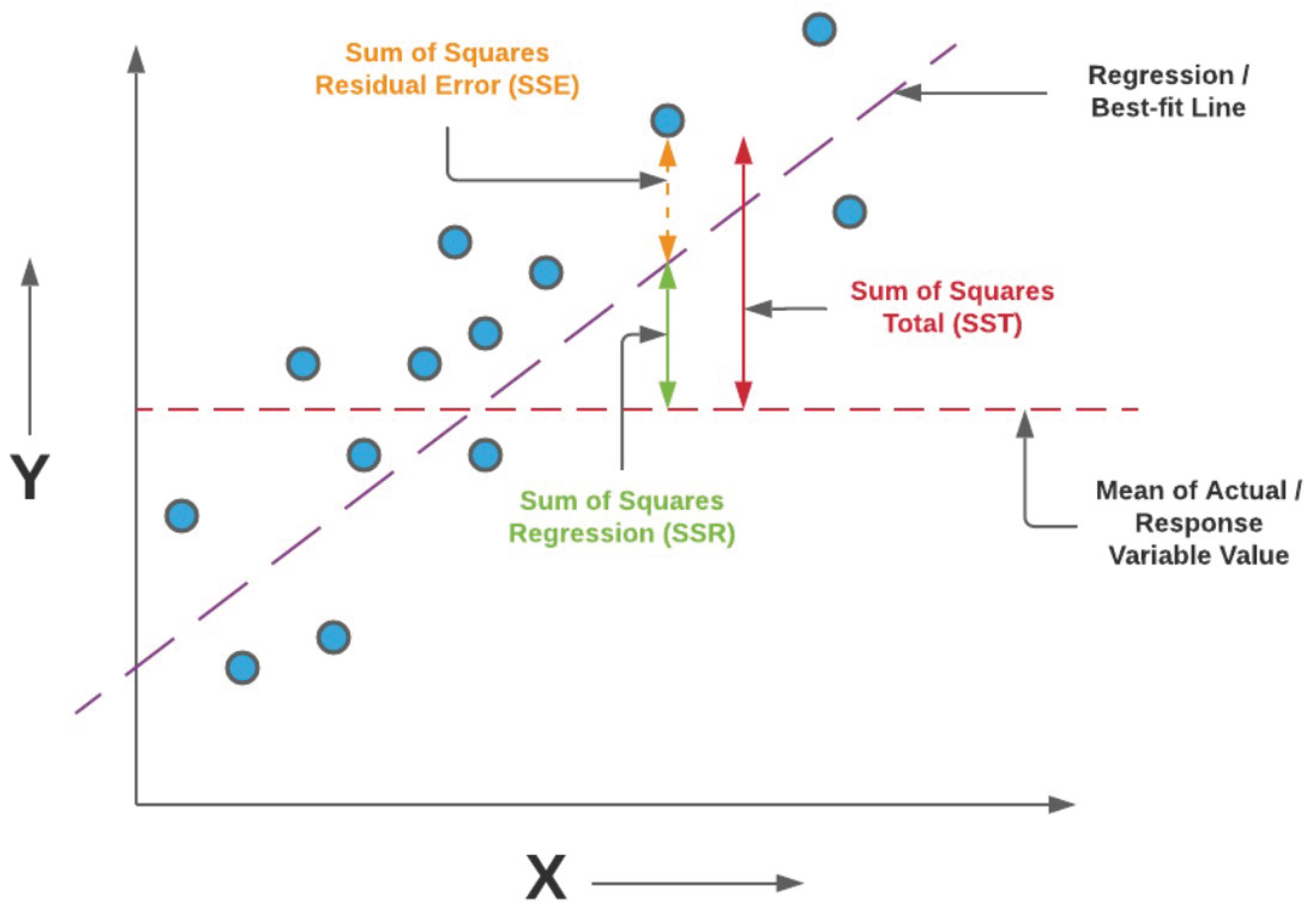
Figure 16.
Illustrative examples of regression performance for different values of the coefficient of determination . Left: High , where predictions closely follow the regression line and most variance is explained. Center: Moderate , indicating partial explanatory power with noticeable dispersion. Right: Low , where predictions exhibit weak alignment with observations and most variance remains unexplained (source: vitaflux.com).
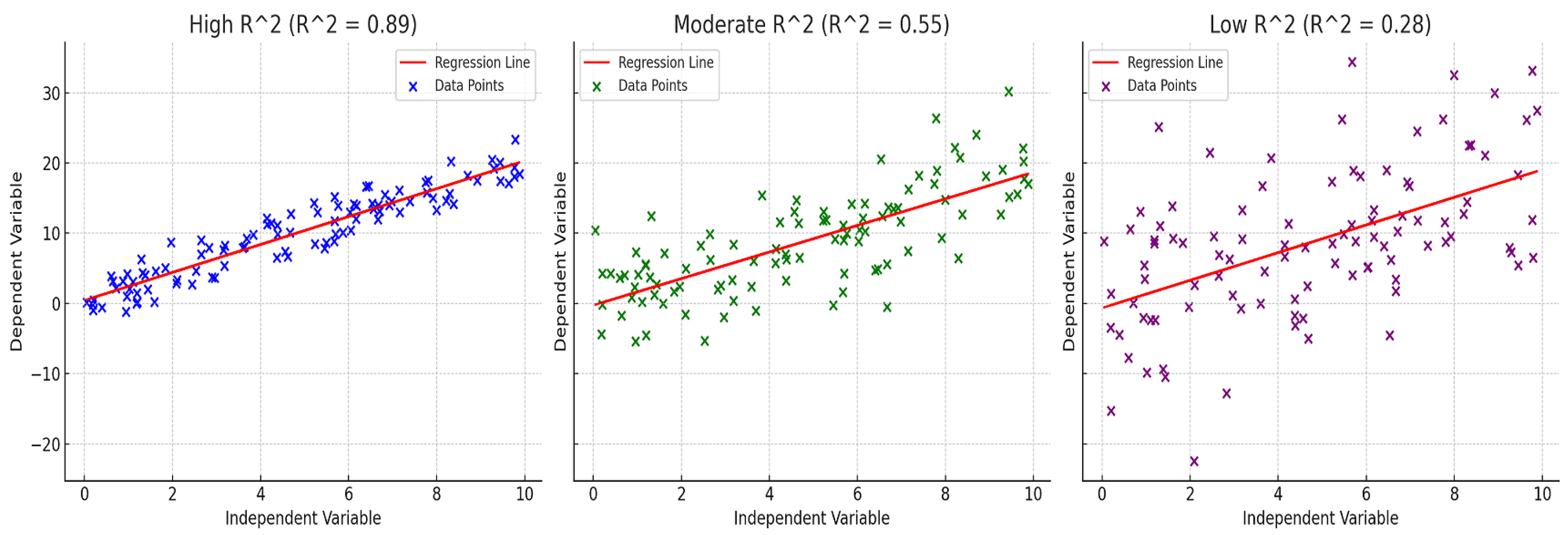
Figure 17.
Illustration of residual errors in a regression model and their contribution to the mean squared error (MSE), which forms the basis of the root mean squared error (RMSE).
Figure 17.
Illustration of residual errors in a regression model and their contribution to the mean squared error (MSE), which forms the basis of the root mean squared error (RMSE).
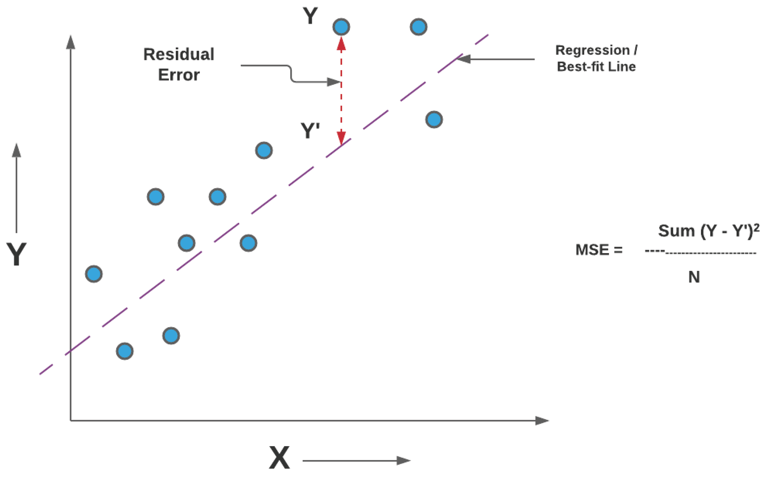
Figure 18.
Overview of the training dataset organization. Ray-tracing simulations are generated across three frequency bands (2.4, 5, and 6 GHz) and four transmit power levels (100, 200, 500, and 1000 mW). Each configuration produces multiple CSV files corresponding to different reflection–diffraction (R/D) settings, forming the complete training data corpus.
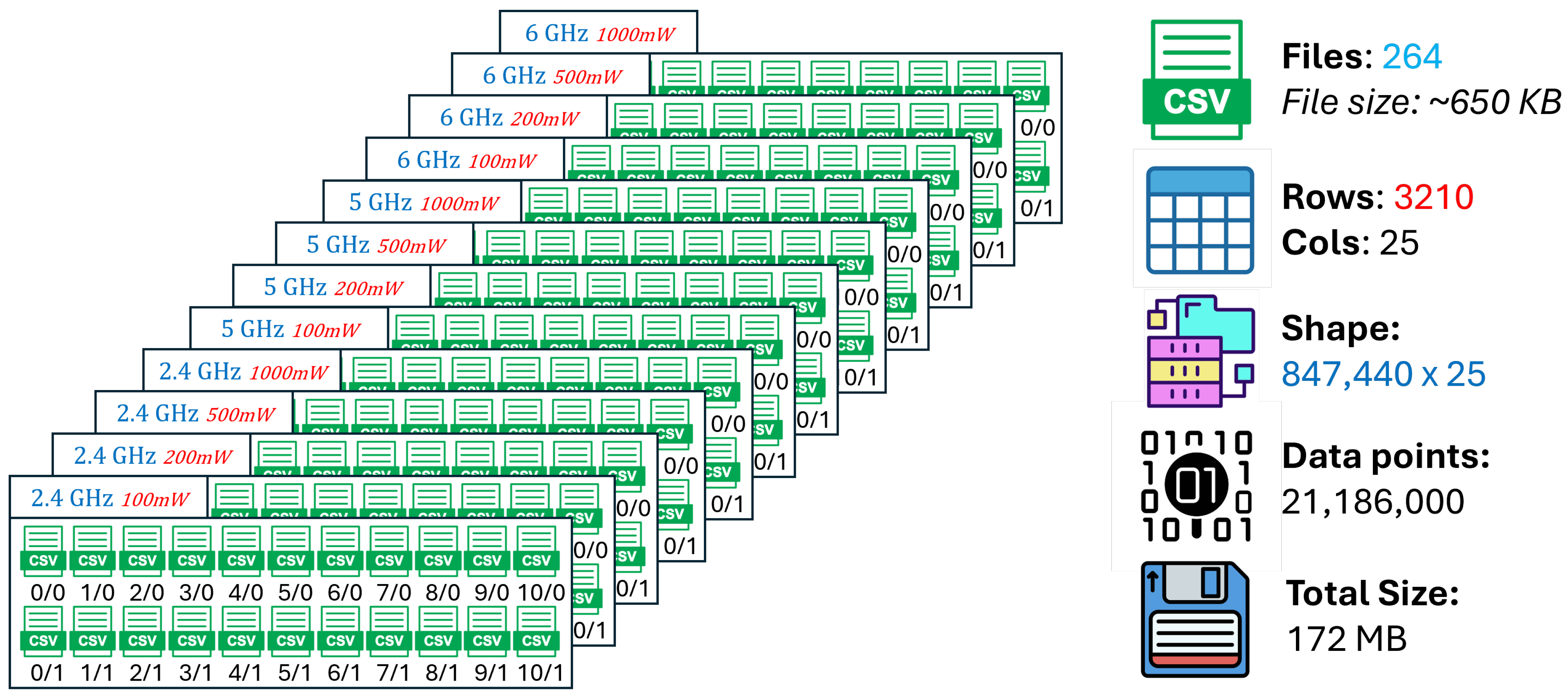
Figure 19.
Organization of the evaluation (validation) dataset. Ray-tracing simulations are generated for three representative channels at 2.4 GHz (2.447 GHz), 5 GHz (5.15 GHz), and 6 GHz (6.905 GHz), all at a fixed transmit power of 1000 mW. Each configuration includes multiple reflection–diffraction (R/D) settings, resulting in a structured set of CSV files used for validation.
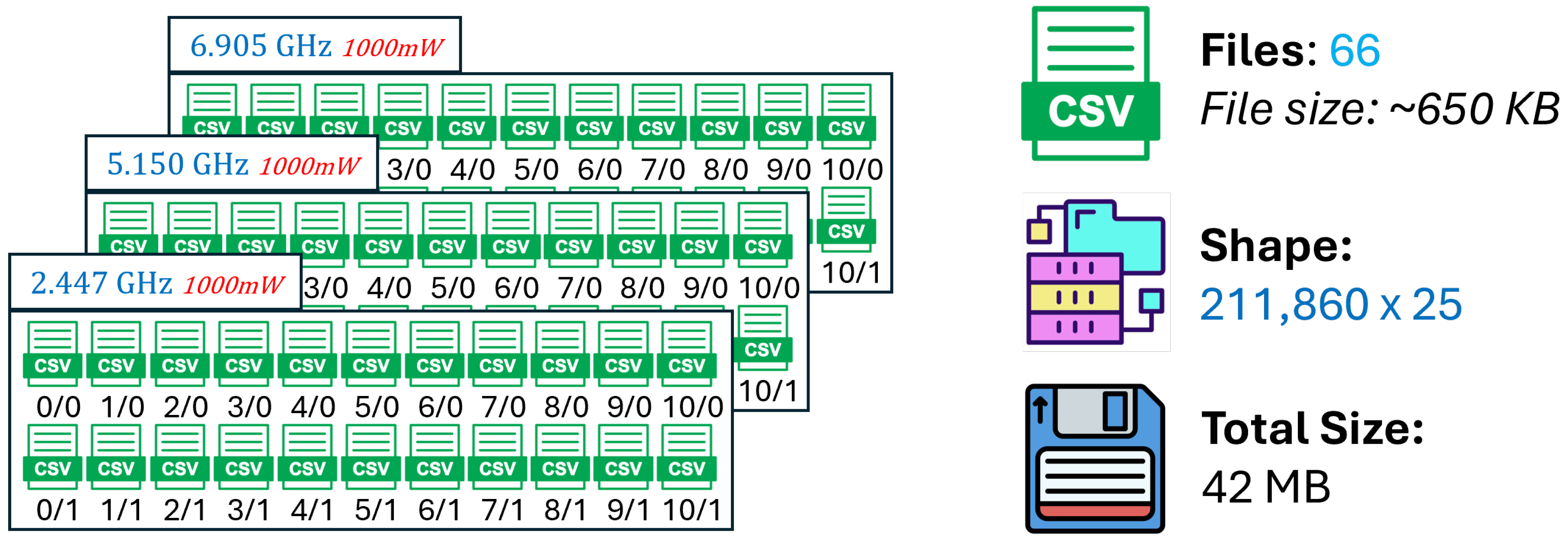
Figure 20.
Organization of the test dataset. High-resolution ray-tracing simulations are generated at 2.447 GHz, 5.15 GHz, and 6.905 GHz, all at a transmit power of 1000 mW, using a finer receiver spacing of 2 m. Each configuration produces a large CSV file containing dense spatial RSSI samples used to assess spatial generalization performance.
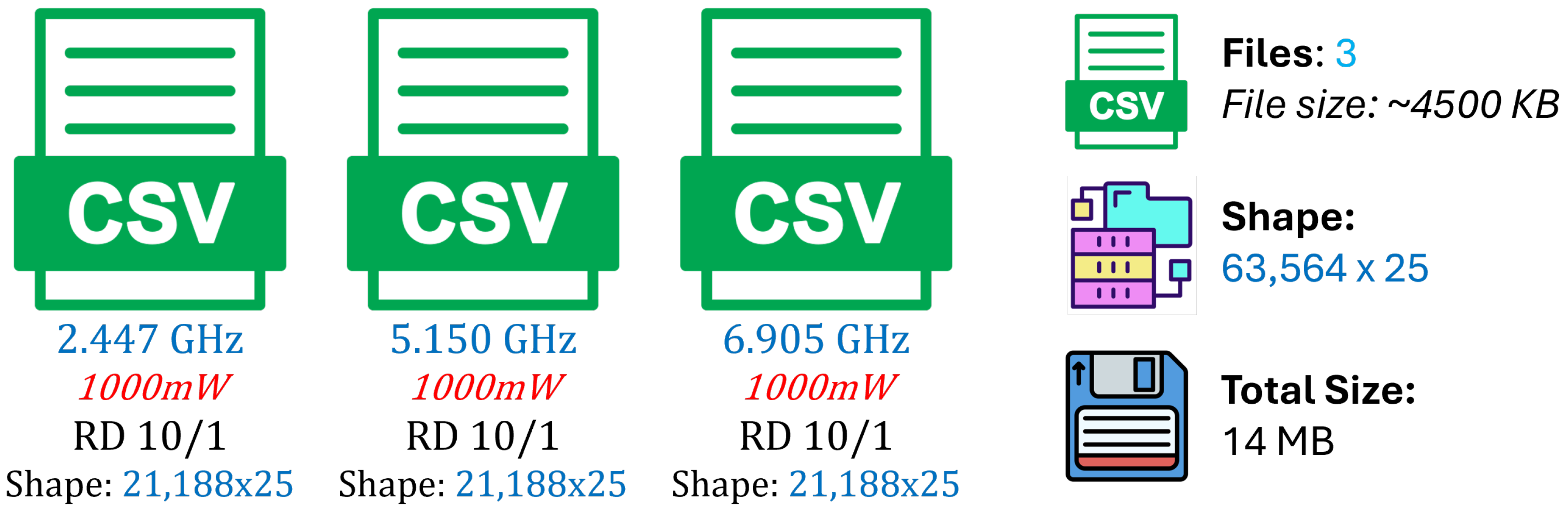
Figure 21.
Overall dataset composition showing the proportion of samples used for training (847,440), validation (211,860), and testing (63,564).
Figure 21.
Overall dataset composition showing the proportion of samples used for training (847,440), validation (211,860), and testing (63,564).
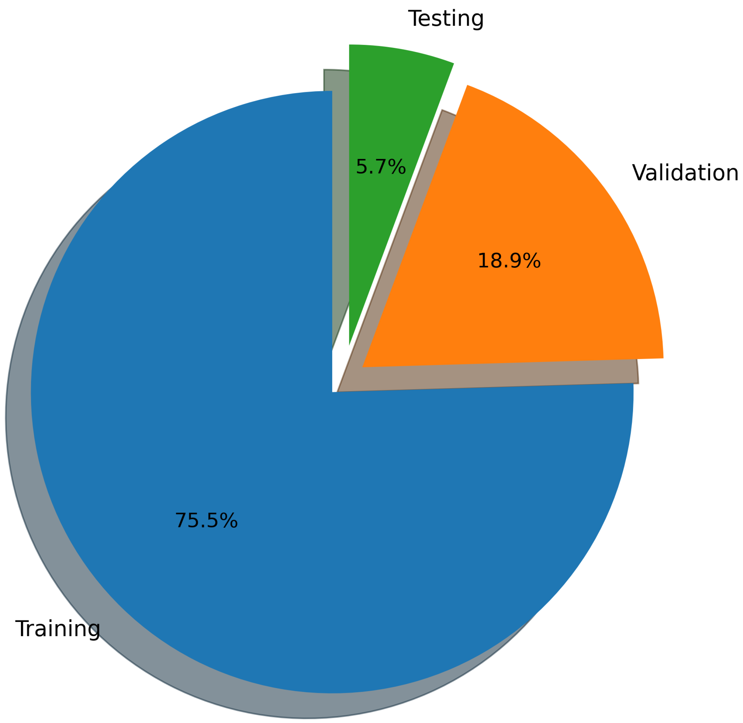
Figure 22.
End-to-end machine learning pipeline for RSSI surrogate modeling. The workflow spans from large-scale ray-tracing data ingestion and preprocessing (Steps 1–2), through feature engineering, model selection, and NAS-based tuning (Steps 3–4), to model training and fast inference (Steps 5–6). Prediction outputs are used for coverage analysis and system-level evaluation (Step 7), with a forward-looking integration into wireless digital twin services and network intelligence applications (Step 8).
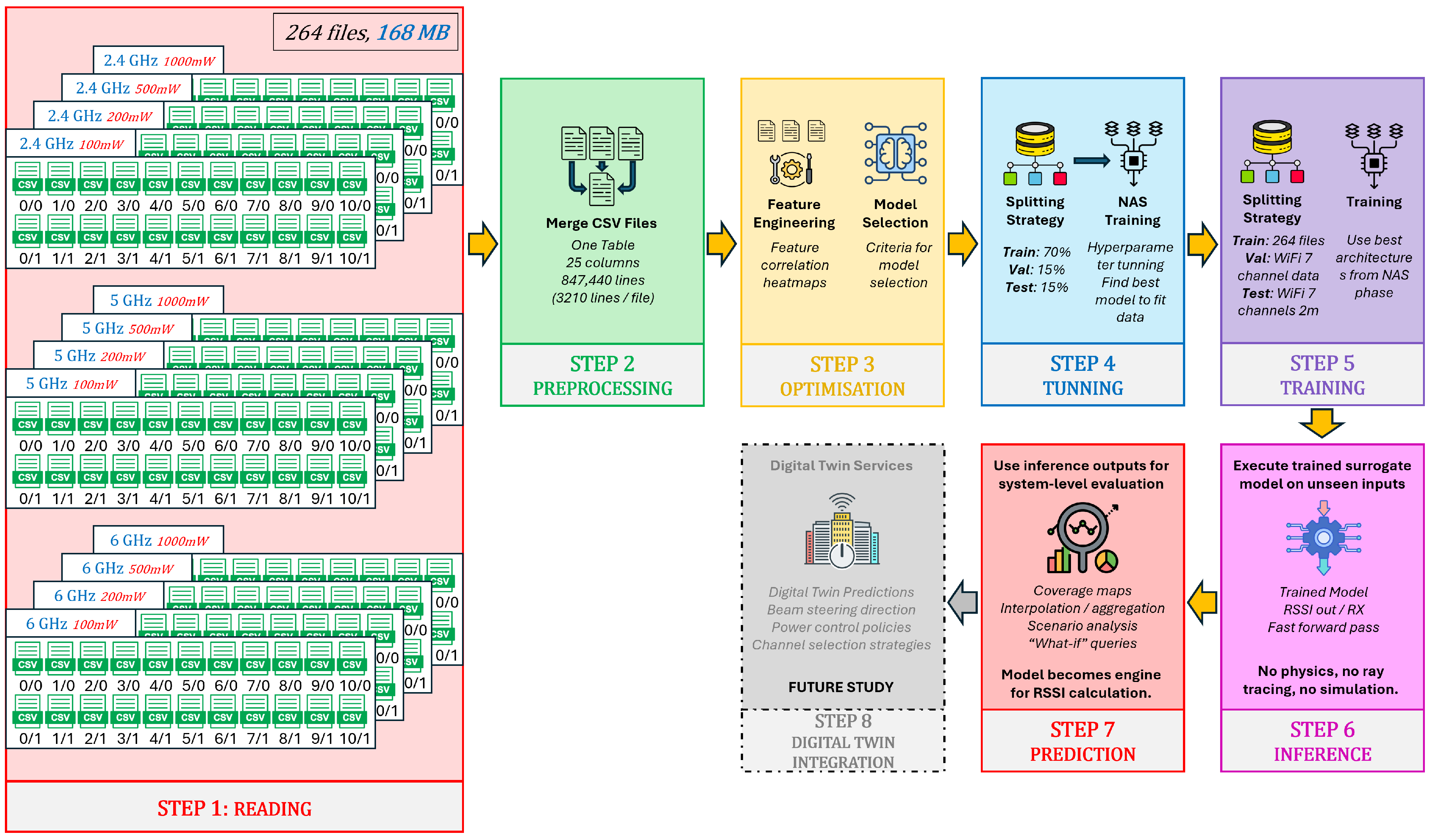
Figure 23.
Feature–target correlation heatmaps showing Pearson, Spearman, and Kendall correlation coefficients between ray-tracing-derived input features and the RSSI targets (RSSI1, RSSI2). Positive and negative correlations reflect physical propagation effects such as transmit power scaling, distance-dependent path loss, frequency-dependent attenuation, and multipath interactions.
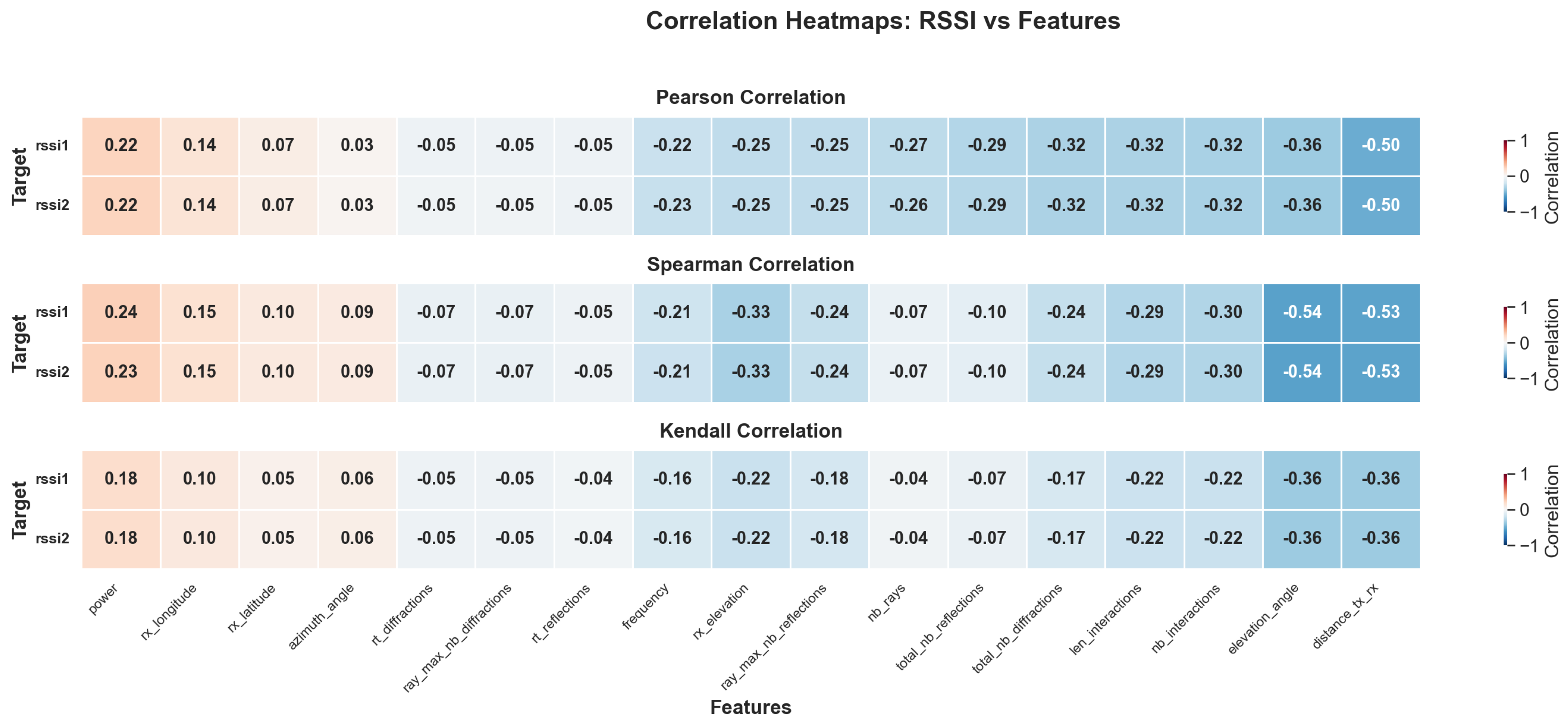
Figure 24.
Signal coverage maps for different ray-tracing configurations, RT 0/0 to RT 2/1, at 5 GHz with a transmission power of 100mW, showing the effects of reflections and diffractions on signal strength in an urban campus setting.
Figure 24.
Signal coverage maps for different ray-tracing configurations, RT 0/0 to RT 2/1, at 5 GHz with a transmission power of 100mW, showing the effects of reflections and diffractions on signal strength in an urban campus setting.
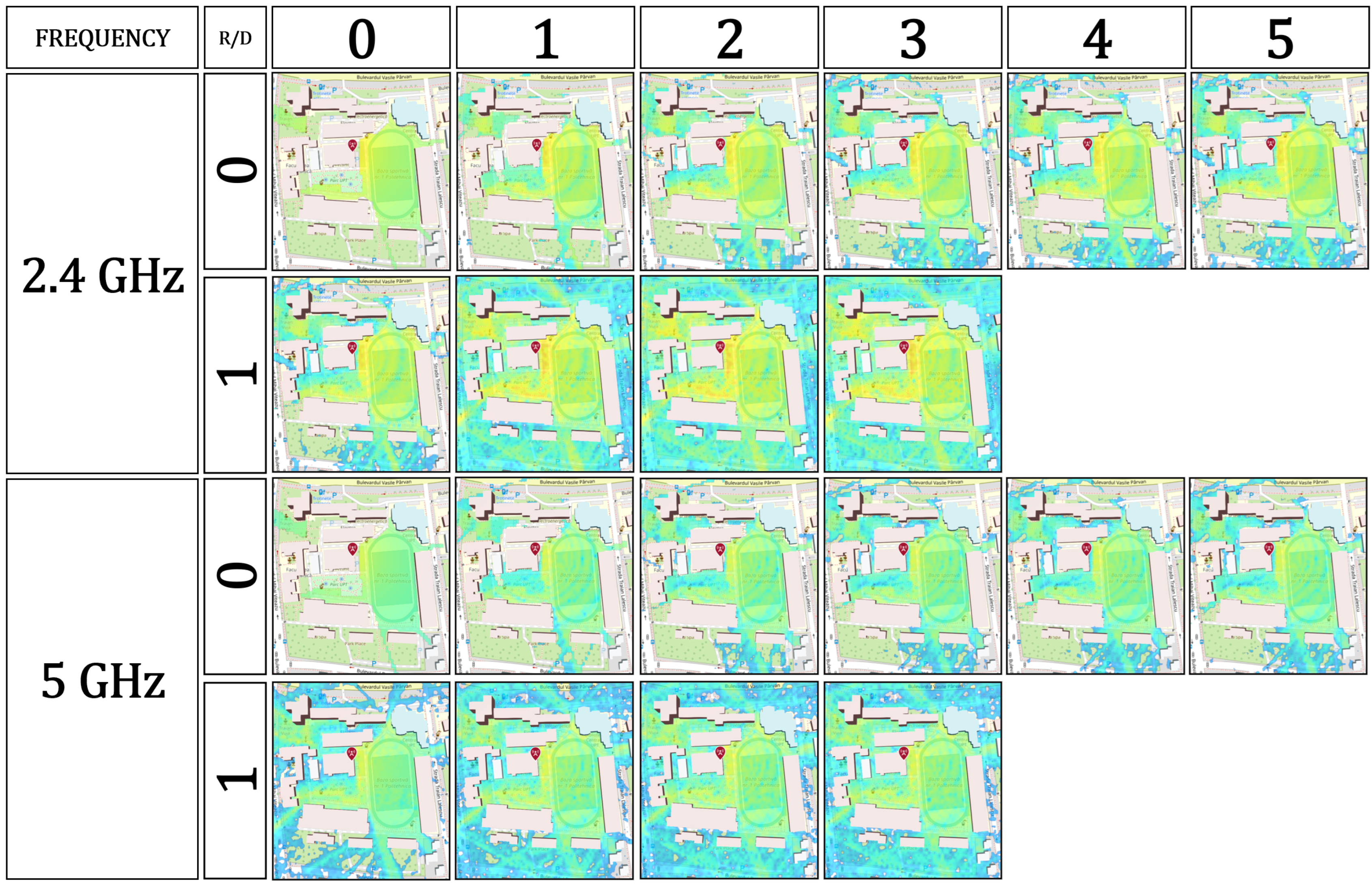
Figure 25.
RSSI versus Tx-Rx distance for 2.4, 5, and 6 GHz aggregated across RT 10/1 ray-tracing configurations and all transmit power levels (100, 200, 500, 1000 mW). Solid lines represent binned-median trends ( bins), and faded points correspond to downsampled individual measurements. Linear regression metrics are intentionally omitted due to the multipath-dominated nature of the dataset.
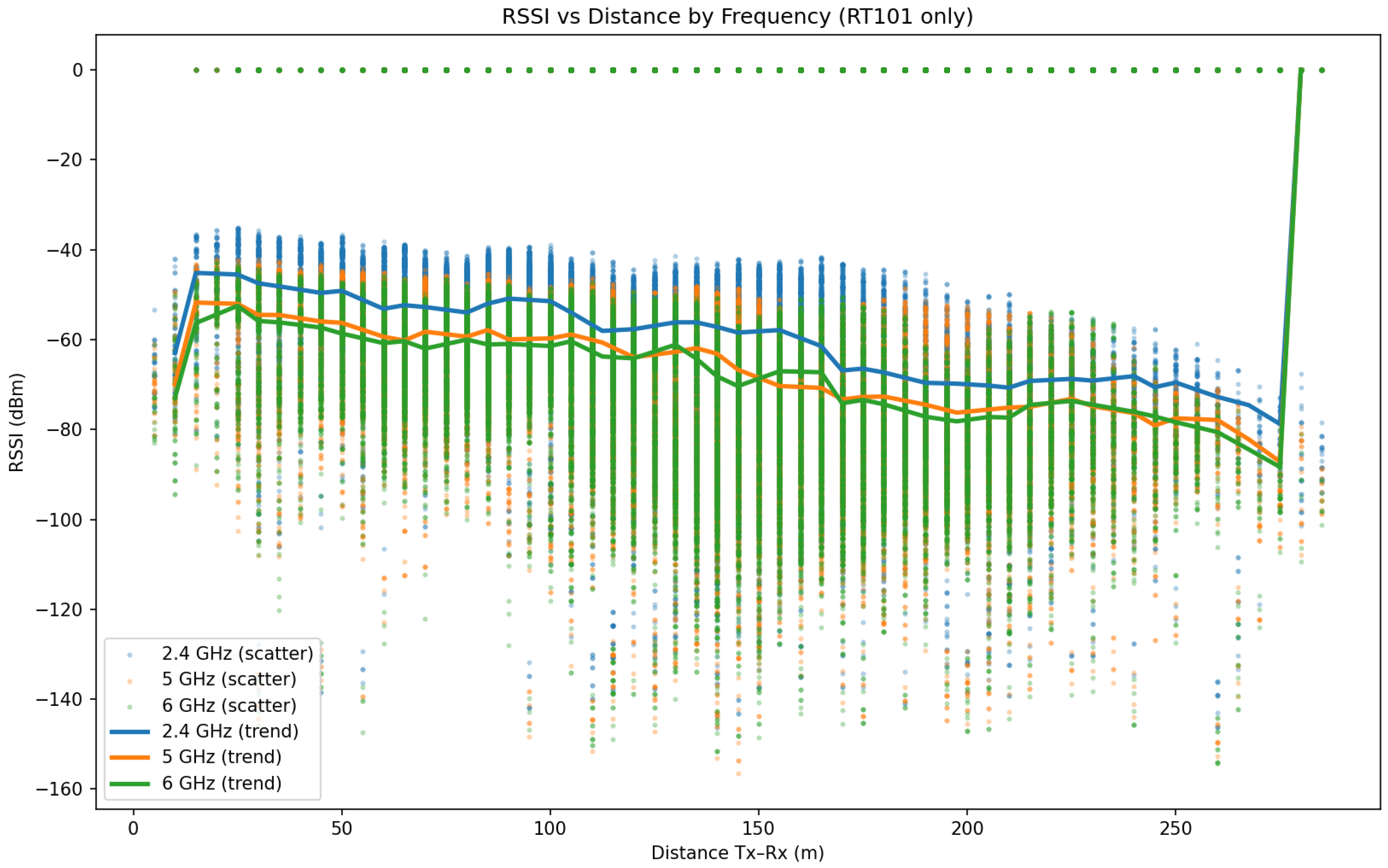
Figure 26.
RSSI as a function of the total number of reflections aggregated across all ray-tracing configurations, receiver locations, transmit power levels, and operating frequencies (2.4, 5, and 6 GHz). Light scatter points represent individual receiver samples, while solid curves indicate the median RSSI per reflection-count bin with interquartile range (IQR) error bars. The figure illustrates the systematic degradation of received signal strength with increasing multipath complexity and highlights frequency-dependent sensitivity to cumulative reflection losses.
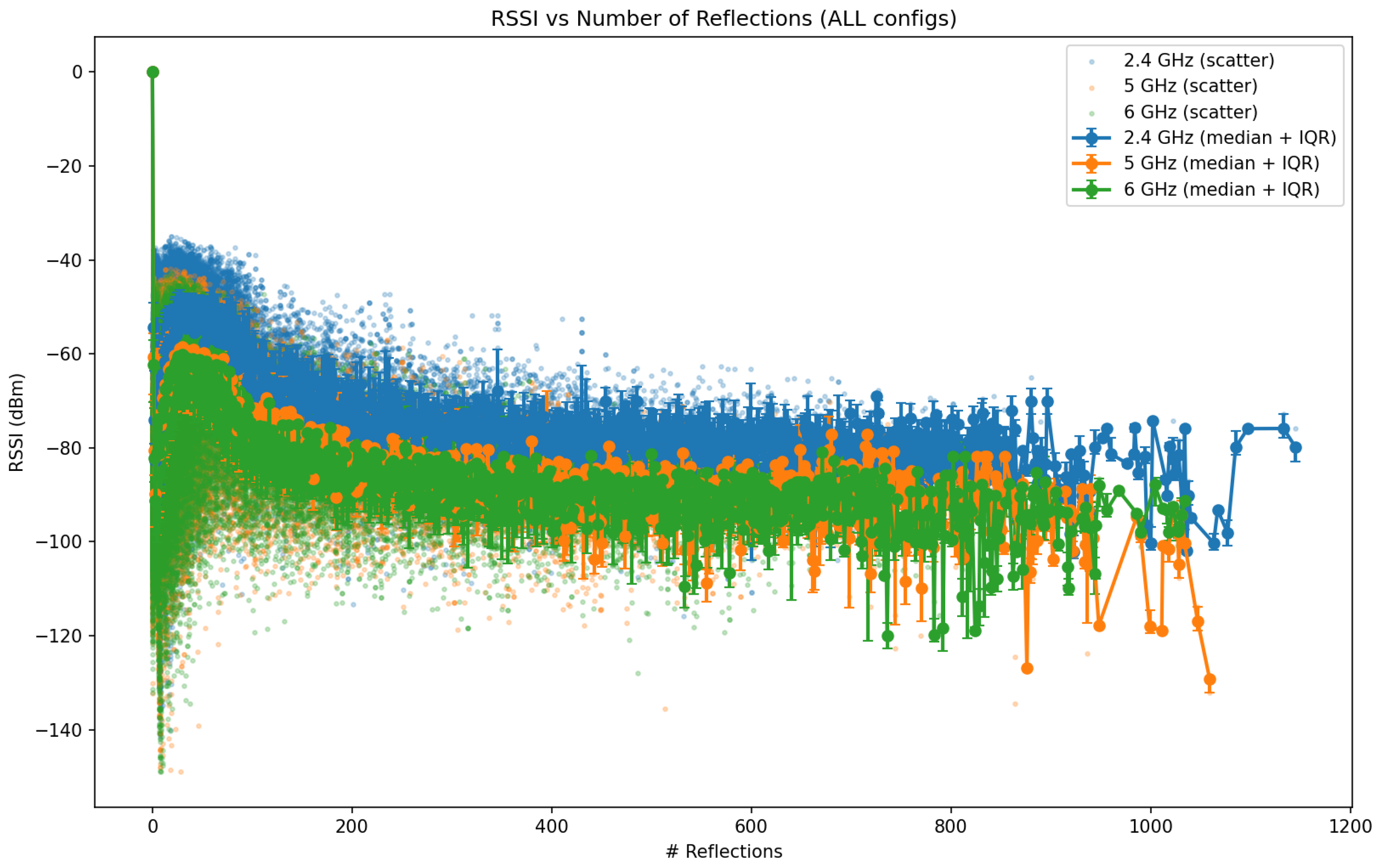
Figure 27.
RSSI versus total number of diffractions aggregated over all ray-tracing configurations and frequencies (2.4, 5, and 6 GHz). Scatter points represent individual samples, while solid curves show the median RSSI with interquartile ranges, highlighting the strong attenuation associated with diffraction-dominated propagation.
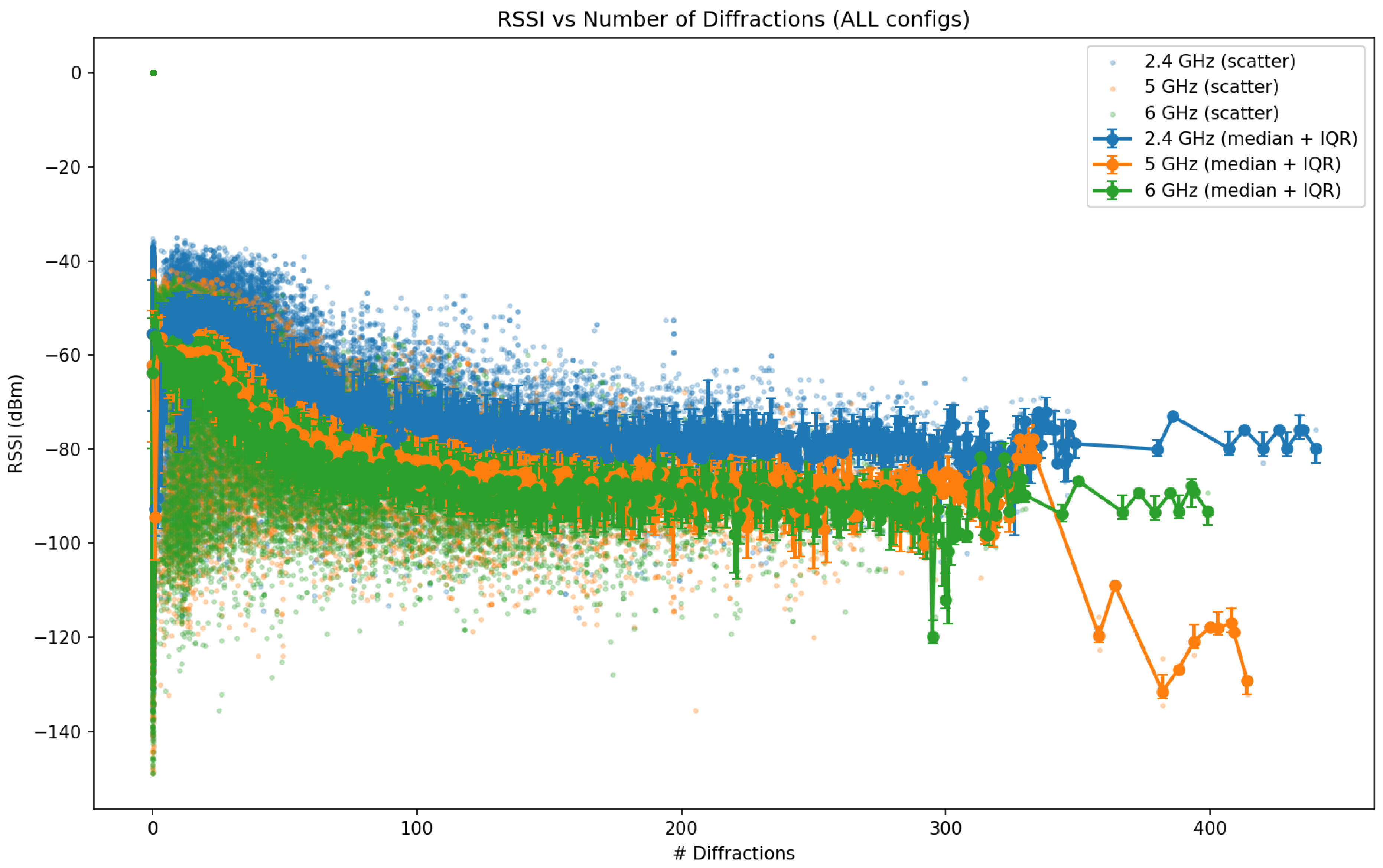
Figure 28.
RSSI distribution across the 2.4 GHz, 5 GHz, and 6 GHz Wi-Fi bands. The top panel shows the normalized 2D histogram of RSSI values, highlighting the central tendency and overlap between frequency bands under identical geometric and environmental conditions. The bottom-left panel presents a 3D scatter plot where each frequency band forms a distinct layer, illustrating the spread and density of individual measurements. The bottom-right panel shows the corresponding 3D histograms with semi-transparent bars to allow direct visual comparison of distribution shapes. Together, these views provide a comprehensive characterization of frequency-dependent signal behavior, revealing that 2.4 GHz yields the strongest and most concentrated RSSI distribution, while 5 GHz and 6 GHz exhibit progressively weaker and more dispersed signal characteristics due to increased attenuation and reduced diffraction efficiency at higher frequencies.
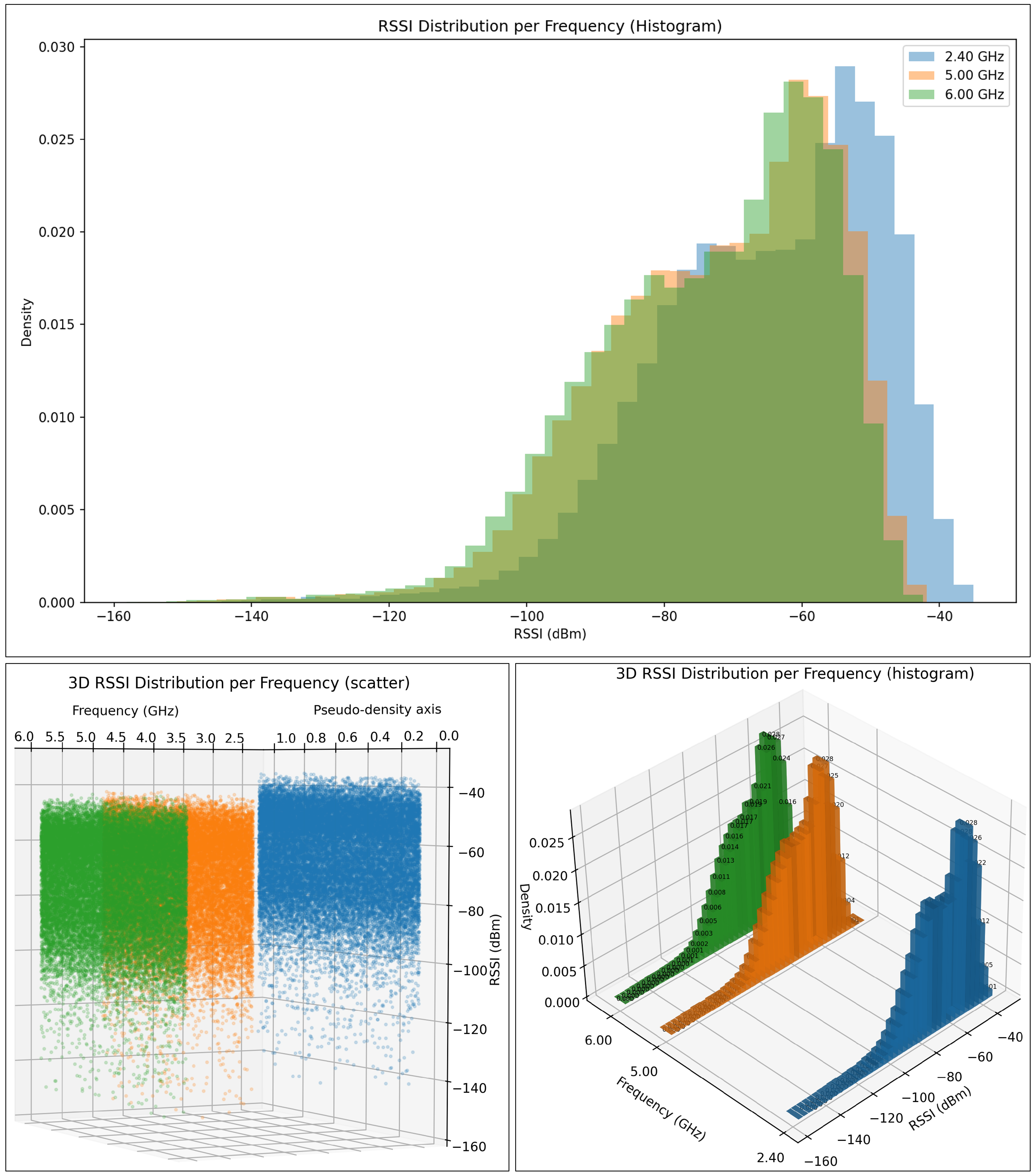
Figure 29.
Comparison of model size and average inference execution time for the RandomForest regressor and the FT-Transformer. The RandomForest model achieves faster per-target inference but requires significantly higher storage (7.7 GB), whereas the FT-Transformer offers a compact model footprint (0.6 MB) at the cost of higher per-target inference latency.
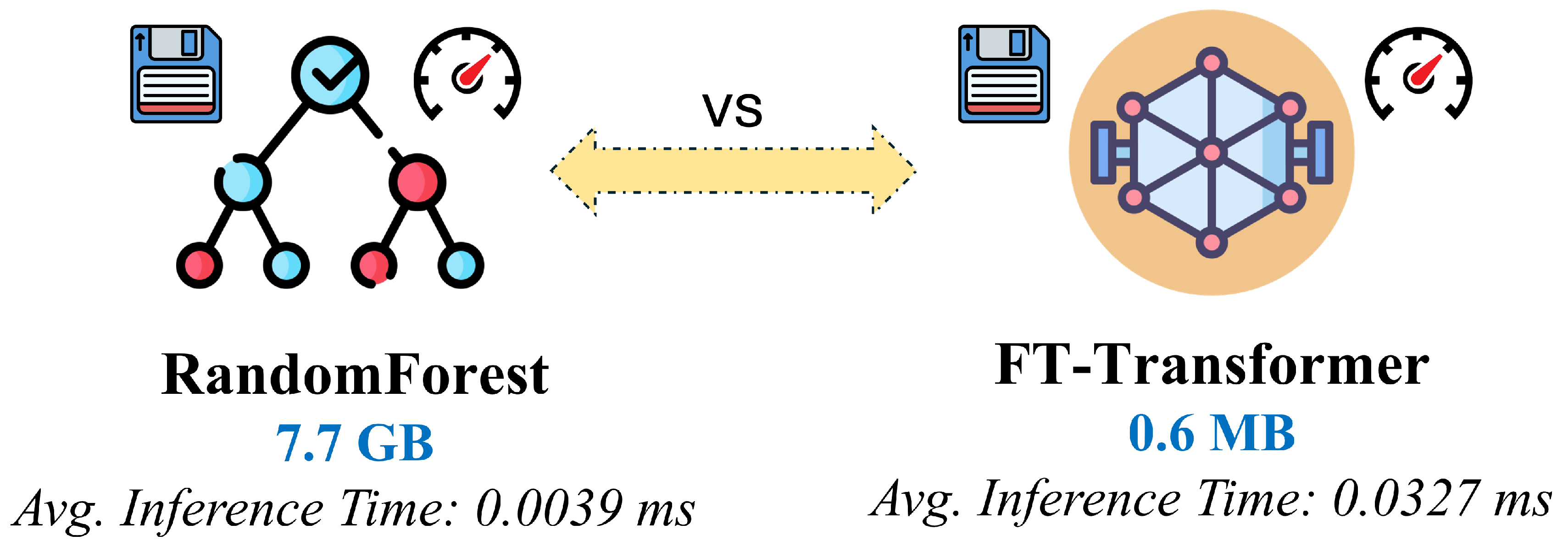
Figure 30.
Comparison between high-fidelity (offline computation, non-real-time simulations) MATLAB ray-tracing data generation and ML–based inference (online real-time computation). The left side illustrates the offline ray-tracing pipeline, where extensive parameter sweeps and multi-ray interactions require weeks/months of computation on dual-CPU servers. The right side highlights the trained FT-Transformer surrogate model, which enables near-instantaneous RSSI prediction through fast forward passes, allowing large-scale coverage analysis and scenario exploration in seconds rather than months.
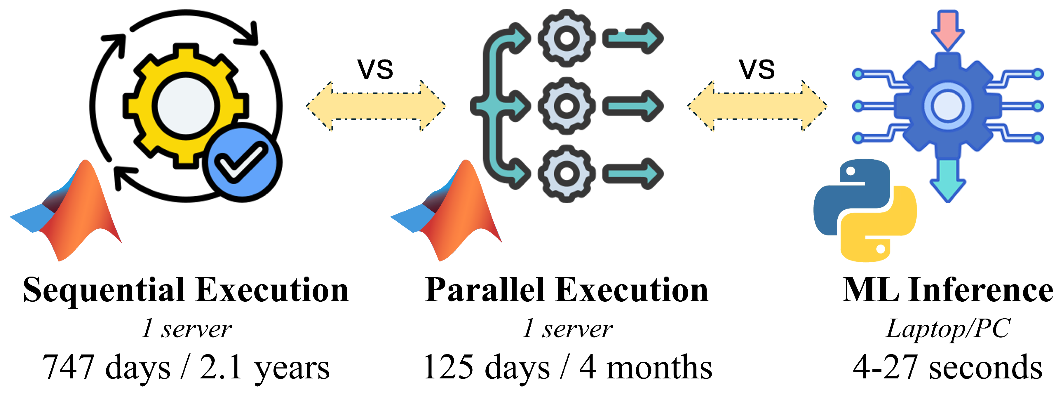
Figure 31.
High-resolution 3D model of the Politehnica University of Timișoara campus, obtained from architectural and LiDAR-based reconstructions. The model includes detailed building geometry and vegetation, enabling more realistic ray-tracing simulations for future studies.
Figure 31.
High-resolution 3D model of the Politehnica University of Timișoara campus, obtained from architectural and LiDAR-based reconstructions. The model includes detailed building geometry and vegetation, enabling more realistic ray-tracing simulations for future studies.
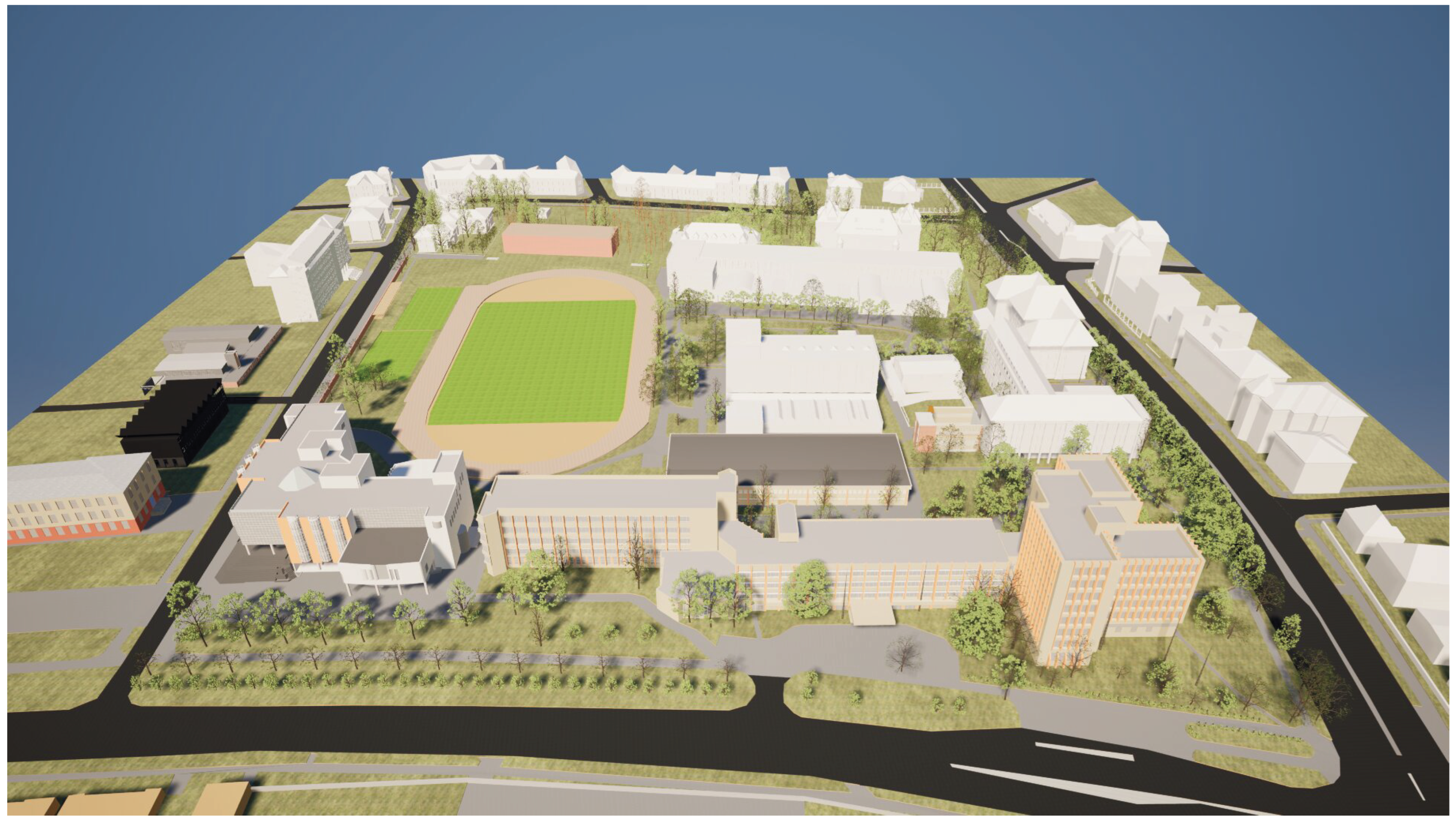
Table 1.
Comparison of QAM Modulation Schemes Used in Wi-Fi Standards
| QAM Order | Bits per Symbol | Approx. Required SNR | Wi-Fi Standard(s) |
|---|---|---|---|
| 4-QAM (QPSK) | 2 | 9 dB | Wi-Fi 1, fallback mode |
| 16-QAM | 4 | 16 dB | Wi-Fi 2–7 |
| 64-QAM | 6 | 24 dB | Wi-Fi 4 (802.11n) |
| 256-QAM | 8 | 30 dB | Wi-Fi 5 (802.11ac) |
| 1024-QAM | 10 | 35 dB | Wi-Fi 6 (802.11ax) |
| 4096-QAM | 12 | 41–43 dB | Wi-Fi 7 (802.11be) |
Table 2.
Statistical summary of RSSI distributions (in dBm) for the 2.4 GHz, 5 GHz, and 6 GHz Wi-Fi bands across all ray-tracing configurations.
Table 2.
Statistical summary of RSSI distributions (in dBm) for the 2.4 GHz, 5 GHz, and 6 GHz Wi-Fi bands across all ray-tracing configurations.
| Frequency [GHz] | Count | Mean | Median | Std | Min | P5 | P25 | P75 | P95 | Max | IQR |
|---|---|---|---|---|---|---|---|---|---|---|---|
| 2.4 | 1,076,698 | -65.05 | -62.82 | 16.06 | -150.12 | -92.96 | -75.96 | -52.16 | -43.93 | -35.06 | 23.80 |
| 5.0 | 1,081,920 | -72.00 | -69.47 | 16.37 | -156.58 | -100.42 | -83.31 | -58.79 | -50.42 | -41.84 | 24.52 |
| 6.0 | 1,049,220 | -73.34 | -70.56 | 16.48 | -158.17 | -102.25 | -84.65 | -60.13 | -51.88 | -42.40 | 24.52 |
Metrics computed over the consolidated ray-tracing dataset using RSSI (dry-propagation) values with fallback to RSSI when missing. Percentiles (, , , ) and the interquartile range (IQR) highlight the spread and tail behavior of received signal strength across frequency bands.
Table 3.
FT-Transformer RSSI [dBm] results over five independent runs. Metrics reported per split; bottom rows show mean and standard deviation across runs.
Table 3.
FT-Transformer RSSI [dBm] results over five independent runs. Metrics reported per split; bottom rows show mean and standard deviation across runs.
| Run | MAE [dBm] | RMSE [dBm] | MAE [dBm] | RMSE [dBm] | MAE [dBm] | RMSE [dBm] | |||
|---|---|---|---|---|---|---|---|---|---|
| 1 | 0.9971 | 0.9962 | 0.9962 | 0.9536 | 1.4632 | 1.0510 | 1.6675 | 1.0502 | 1.6670 |
| 2 | 0.9967 | 0.9958 | 0.9958 | 1.0158 | 1.5602 | 1.1067 | 1.7559 | 1.1093 | 1.7494 |
| 3 | 0.9969 | 0.9960 | 0.9960 | 0.9936 | 1.5124 | 1.0872 | 1.7178 | 1.0858 | 1.7153 |
| 4 | 0.9976 | 0.9968 | 0.9968 | 0.8735 | 1.3382 | 0.9579 | 1.5333 | 0.9576 | 1.5252 |
| 5 | 0.9974 | 0.9966 | 0.9967 | 0.9045 | 1.3849 | 0.9908 | 1.5795 | 0.9903 | 1.5654 |
| Mean | 0.9971 | 0.9963 | 0.9963 | 0.9482 | 1.4518 | 1.0387 | 1.6508 | 1.0386 | 1.6445 |
| Std | 0.00036 | 0.00041 | 0.00044 | 0.05948 | 0.09074 | 0.06315 | 0.09314 | 0.06375 | 0.09619 |
Each run was trained for up to 500 epochs. A new random 70/15/15 data split (train/validation/test) was generated for every run, ensuring statistical independence across experiments. The best model was selected (among the 500 epochs) based on maximum training .
Table 4.
RandomForestRegressor RSSI [dBm] results over five independent runs. Metrics reported per split; bottom rows show mean and standard deviation across runs.
Table 4.
RandomForestRegressor RSSI [dBm] results over five independent runs. Metrics reported per split; bottom rows show mean and standard deviation across runs.
| Run | MAE [dBm] | RMSE [dBm] | MAE [dBm] | RMSE [dBm] | MAE [dBm] | RMSE [dBm] | |||
|---|---|---|---|---|---|---|---|---|---|
| 1 | 0.9993 | 0.9947 | 0.9947 | 0.3329 | 0.7318 | 0.9017 | 1.9685 | 0.8946 | 1.9625 |
| 2 | 0.9993 | 0.9947 | 0.9946 | 0.3337 | 0.7332 | 0.9029 | 1.9695 | 0.8975 | 1.9676 |
| 3 | 0.9993 | 0.9947 | 0.9946 | 0.3334 | 0.7331 | 0.9017 | 1.9669 | 0.8969 | 1.9681 |
| 4 | 0.9993 | 0.9947 | 0.9947 | 0.3326 | 0.7316 | 0.9011 | 1.9676 | 0.8952 | 1.9624 |
| 5 | 0.9993 | 0.9947 | 0.9946 | 0.3334 | 0.7335 | 0.9019 | 1.9683 | 0.8956 | 1.9669 |
| Mean | 0.9993 | 0.9947 | 0.9946 | 0.3334 | 0.7331 | 0.9017 | 1.9683 | 0.8956 | 1.9669 |
| Std | 0.00000 | 0.00000 | 0.00005 | 0.00044 | 0.00087 | 0.00065 | 0.00098 | 0.00121 | 0.00282 |
Each run was trained for up to 500 epochs. A new random 70/15/15 data split (train/validation/test) was generated for every run, ensuring statistical independence across experiments. The best model was selected (among the 500 epochs) based on maximum training .
Table 5.
Comparison of FT-Transformer and RandomForestRegressor on RSSI [dBm] prediction. Values shown are mean ± standard deviation over five independent runs.
Table 5.
Comparison of FT-Transformer and RandomForestRegressor on RSSI [dBm] prediction. Values shown are mean ± standard deviation over five independent runs.
| Model | MAE | RMSE | MAE | RMSE | MAE | RMSE | |||
|---|---|---|---|---|---|---|---|---|---|
| FT-Transformer | |||||||||
| RF-Regressor |
Table 6.
FT-Transformer fine-tuning results for RSSI prediction [dBm] over five independent runs using a fixed file-based split.
Table 6.
FT-Transformer fine-tuning results for RSSI prediction [dBm] over five independent runs using a fixed file-based split.
| Run | MAE | RMSE | MAE | RMSE | MAE | RMSE | |||
|---|---|---|---|---|---|---|---|---|---|
| Run #1 | 0.9955 | 0.9532 | 0.8003 | 1.1605 | 1.7763 | 3.5178 | 5.3811 | 4.7906 | 6.5370 |
| Run #2 | 0.9953 | 0.9536 | 0.8041 | 1.1860 | 1.8130 | 3.4920 | 5.3570 | 4.7410 | 6.4750 |
| Run #3 | 0.9968 | 0.9559 | 0.8103 | 0.9734 | 1.5080 | 3.3892 | 5.2230 | 4.6377 | 6.3727 |
| Run #4 | 0.9955 | 0.9532 | 0.8003 | 1.6052 | 1.7763 | 3.5178 | 5.3811 | 4.7906 | 6.5371 |
| Run #5 | 0.9954 | 0.9564 | 0.8074 | 1.1646 | 1.7955 | 3.3962 | 5.1931 | 4.7101 | 6.4201 |
| Avg | 0.9955 | 0.9536 | 0.8041 | 1.1646 | 1.7763 | 3.4920 | 5.3570 | 4.7410 | 6.4750 |
| Std | 0.00062 | 0.00156 | 0.00440 | 0.23288 | 0.12716 | 0.06472 | 0.09153 | 0.06384 | 0.07239 |
Disclaimer/Publisher’s Note: The statements, opinions and data contained in all publications are solely those of the individual author(s) and contributor(s) and not of MDPI and/or the editor(s). MDPI and/or the editor(s) disclaim responsibility for any injury to people or property resulting from any ideas, methods, instructions or products referred to in the content. |
© 2026 by the authors. Licensee MDPI, Basel, Switzerland. This article is an open access article distributed under the terms and conditions of the Creative Commons Attribution (CC BY) license (http://creativecommons.org/licenses/by/4.0/).
Copyright: This open access article is published under a Creative Commons CC BY 4.0 license, which permit the free download, distribution, and reuse, provided that the author and preprint are cited in any reuse.


