1. Introduction
Estimating actual evapotranspiration (ETa) is critically important for effective water resource management and agricultural irrigation planning. Accurate ETa determination is essential for correctly modeling the hydrological cycle and developing sustainable agricultural water management strategies. In recent years, energy balance-based methods have been developed to estimate crop water consumption, leveraging the spatial information provided by remote sensing data. Notable examples include SEBAL (Surface Energy Balance Algorithm for Land) [
1], METRIC (Mapping Evapotranspiration at High Resolution with Internalized Calibration) [
2], and SSEB (Simplified Surface Energy Balance) [
3].
In addition to these models, Teixeira [
4] proposed the SAFER (Simple Algorithm for Evapotranspiration Retrieving) algorithm, which is both biophysically realistic and computationally efficient, particularly for irrigated areas in semi-arid regions. SAFER calculates the evapotranspiration fraction (ETf = ETa/ETo) using remote sensing variables such as the Normalized Difference Vegetation Index (NDVI), spectral reflectance bands, land surface temperature, and basic meteorological data. By integrating vegetation characteristics with surface energy balance parameters and Penman–Monteith-based reference evapotranspiration (ETo), SAFER provides a comprehensive and practical method for determining the spatial distribution of ETa [
5,
6,
7,
8,
9].
The Penman–Monteith equation is a widely adopted standard approach for calculating ETo. However, in cases where the required meteorological data are missing or unavailable, simpler empirical methods are sometimes employed [
10,
11,
12,
13,
14,
15]. While most SAFER-based studies determine ETo using the Penman–Monteith method [
7,
16], applications relying on simpler approaches remain limited [
6].
SAFER is commonly favored for ETa estimation because it requires only a few remote sensing inputs—such as NDVI, surface temperature, and surface albedo—that are directly linked to physical processes. The data needed for the model include reflectance values from Landsat-8 blue (B2), green (B3), red (B4), near-infrared (B5), and shortwave infrared bands (B6–B7), along with brightness temperatures derived from the thermal bands (B10–B11) [
17]. Numerous studies have shown that SAFER can be effectively applied at daily and monthly scales across different climates and land use types.
Recent applications have highlighted SAFER’s potential to improve irrigation efficiency [
18,
19,
20]. For instance, Nadeem et al. [
18] identified over-irrigated areas in Pakistan, achieving up to 81% groundwater savings, while Do Nascimento Leão et al. [
19] reported similar benefits in citrus orchards in the Amazon. Venancio et al. [
20] demonstrated that recalibrating SAFER coefficients in Brazil’s semi-arid regions significantly improved model accuracy (r = 0.91, RMSE = 0.469 mm/day). These studies underscore that SAFER coefficients are sensitive to regional conditions and that site-specific calibration is crucial [
18,
19,
20,
21,
22].
A commonly used calibration approach involves transforming the SAFER equation into a linear form through logarithmic conversion and estimating parameters using the least squares method. However, this method often exhibits noticeable performance drops during dry periods [
23]. Lopez et al. reported high accuracy during wet seasons but increased parameter sensitivity and weakened ETa predictions during dry periods. This issue has been linked to the inability of vegetation indices like NDVI to fully capture water stress and to the limitations of linear calibration techniques. Consequently, there has been growing interest in heuristic and more flexible computational approaches.
In this context, Karahan et al. [
24] developed a new artificial neural network (ANN) model for daily ETa estimation using NDVI, land surface temperature, and limited meteorological data. Despite being trained on only 38 Landsat overpass days, the model achieved high accuracy on test data (R² = 0.75–0.76) and showed strong agreement with ETa-METRIC estimates.
Building on existing methods in the literature, this study proposes a holistic and interpretable framework for modeling ETa using remote sensing data, complemented by the heuristic recalibration of SAFER coefficients. A family of four parametric formulations—two linear and two nonlinear—was developed. Linear models represent the ETa–surface parameter relationship in a straightforward manner, while nonlinear models are designed to capture the naturally curvilinear physical interactions between surface temperature, vegetation development, radiation balance, and atmospheric conditions.
Accordingly, this study investigates: (i) whether heuristic optimization of SAFER coefficients improves model performance, (ii) whether physically representative nonlinear formulations provide more stable results than linear methods under low-overpass sensors such as Landsat, and (iii) the sensitivity of the developed models to seasonal variations between wet and dry periods. The results indicate that the proposed models are easier to apply and interpret than black-box approaches such as neural networks, and that ETa predictions for days without satellite overpasses are consistent with those of Karahan et al. [
24].
Overall, this study aims to enhance SAFER performance by recalibrating its coefficients using a heuristic approach and to determine optimal parameters for four newly proposed ETa equations—two linear and two nonlinear. Furthermore, the results of both model groups are compared with four widely used machine learning methods—Random Forest (RF), Bagged Trees (BT), Support Vector Machines (SVM), and Generalized Additive Models (GAM)—to provide a modular, physically based, and easily applicable modeling framework.
2. Materials and Methods
2.1. Study Area and Data Used
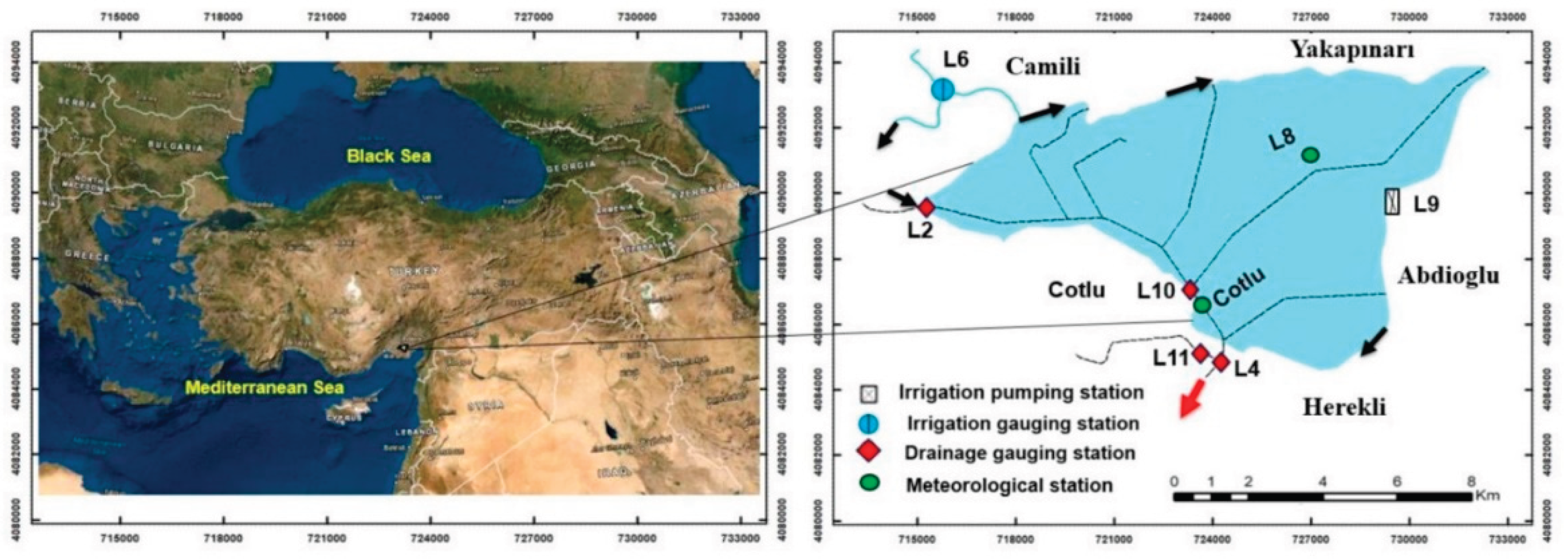
The study area is located in the Lower Seyhan Plain (LSP), situated in the southeastern part of the Mediterranean Region of Türkiye (
Figure 1). The site is approximately 30 km from the city center of Adana and covers an area of 9,495 hectares. The LSP represents a typical delta plain characterized by a highly flat topography with slopes of 1% or less, and an extensive irrigation and drainage network [
24,
25]. In this region, two cropping seasons are practiced each year—summer and winter—dominated mainly by citrus and other rotational crops [
26].
Meteorological data used in this study were obtained from the L8 and Cotlu meteorological stations within the study area [
24,
26]. These data include daily measurements of minimum and maximum air temperature (Tmin, Tmax), wind speed (U), solar radiation (Rs), minimum and maximum relative humidity (RHmin, RHmax), and precipitation (P). The dataset covers 769 consecutive daily observations from September 16, 2020, to October 24, 2022 [
24]. Reference evapotranspiration (ETo, mm day⁻¹) was calculated using the FAO-56 Penman–Monteith method [
27].
According to Equation (1), the variables are defined as follows: ETo (mm day⁻¹) represents reference evapotranspiration; Rn (MJ m⁻² day⁻¹) denotes net radiation; G (MJ m⁻² day⁻¹) is the soil heat flux; (es − ea) indicates the vapor pressure deficit in the air (kPa); γ is the psychrometric constant (kPa °C⁻¹); Δ represents the slope of the saturated vapor pressure–temperature curve (kPa °C⁻¹); u₂ (m s⁻¹) is the wind speed measured at 2 m above ground; and T (°C) is the daily mean air temperature, calculated as the average of daily minimum and maximum temperatures.
Satellite data required for estimating actual evapotranspiration (ETa) and applying the METRIC model were obtained from the United States Geological Survey (USGS) web platform (
http://earthexplorer.usgs.gov) [
2,
28]. Additionally, normalized difference vegetation index (NDVI) and land surface temperature (LST) parameters derived from the MODIS dataset were compiled using the Google Earth Engine (GEE) platform [
29,
30,
31] and harmonized with the dataset employed by Karahan et al. [
24]. This approach ensures that the results produced by the proposed model can be directly compared with the ANN-based model presented by Karahan et al. [
24].
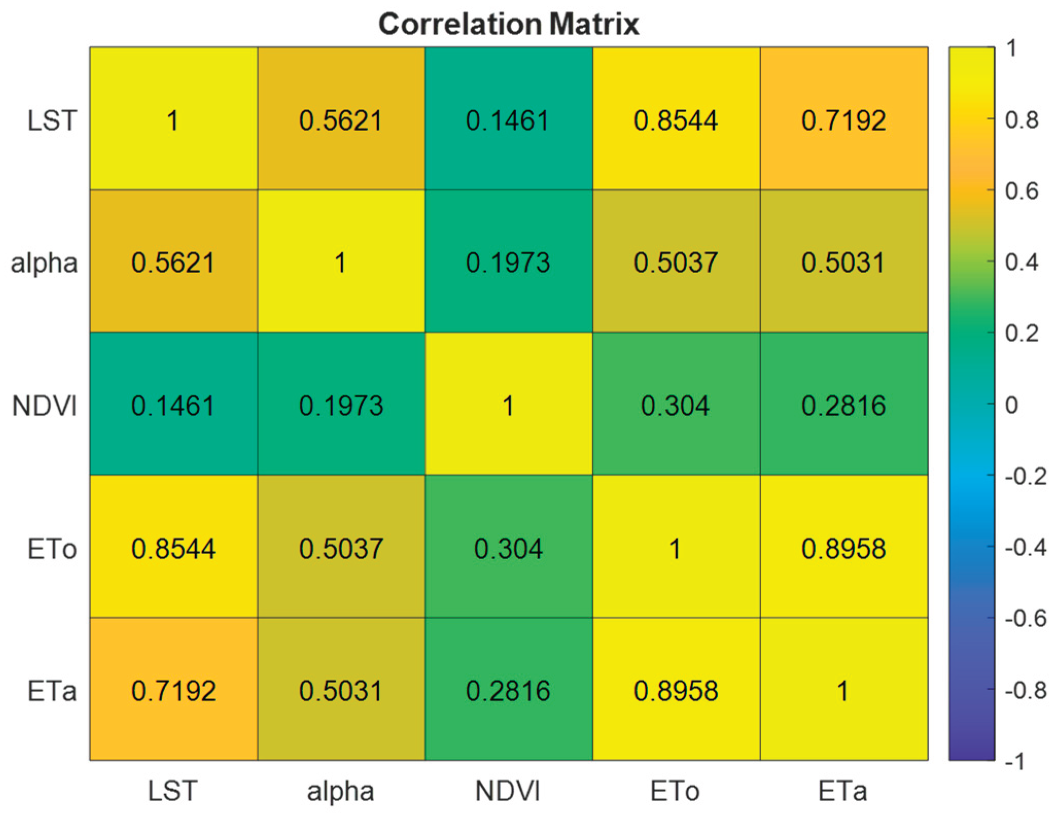
To evaluate linear relationships between the independent variables (LST, albedo, NDVI, ETo) and the dependent variable (ETa), a Pearson correlation matrix was constructed, and the results are summarized in
Figure 2.
According to Equation (1), the variables are defined as follows: ETo (mm day⁻¹) represents reference evapotranspiration; Rn (MJ m⁻² day⁻¹) denotes net radiation; G (MJ m⁻² day⁻¹) is the soil heat flux; (es − ea) represents the vapor pressure deficit in the air (kPa); γ is the psychrometric constant (kPa °C⁻¹); Δ is the slope of the saturated vapor pressure–temperature curve (kPa °C⁻¹); u₂ (m s⁻¹) is the wind speed measured at 2 m above ground; and T (°C) is the daily mean air temperature, calculated as the average of daily minimum and maximum temperatures.
Satellite data required for estimating actual evapotranspiration (ETa) and applying the METRIC model were obtained from the United States Geological Survey (USGS) web platform (
http://earthexplorer.usgs.gov) [
2,
28]. Additionally, normalized difference vegetation index (NDVI) and land surface temperature (LST) parameters derived from the MODIS dataset were compiled via the Google Earth Engine (GEE) platform [
29,
30,
31] and harmonized with the dataset used by Karahan et al. [
24]. This approach ensures that the results produced by the proposed model can be directly compared with the ANN-based model presented by Karahan et al. [
24].
To assess the linear relationships between the independent variables (LST, albedo, NDVI, ETo) and the dependent variable (ETa), a Pearson correlation matrix was constructed, and the results are summarized in
Figure 2.
The correlation analysis revealed that ETa has a very strong positive correlation with ETo (r = 0.896), a high positive correlation with LST (r = 0.719), and a moderate positive correlation with albedo (r = 0.503). The correlation with NDVI was relatively weak (r = 0.282); however, NDVI was found to effectively capture seasonal variations in vegetation and was therefore included as an auxiliary variable in the model. These findings indicate that ETo is the strongest determinant of ETa, LST plays a significant role in capturing the temporal and thermal dynamics of evapotranspiration, and albedo provides additional information on surface reflectance, moderately enhancing model performance.
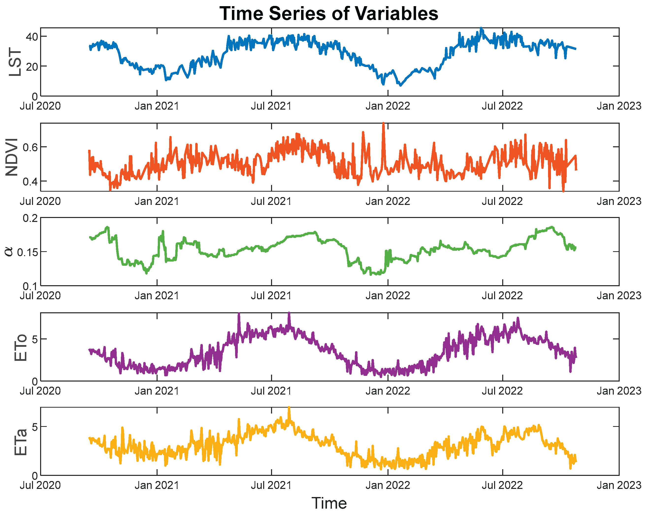
Figure 3 presents the temporal variations of the model inputs and ETa values. The combined evaluation of
Figure 2 and
Figure 3 confirms the strong relationships between ETa and the examined variables. Based on these findings, the model selection and design process is described in detail in the following section. In
Figure 3, ETo and ETa are shown in mm/day, LST in °C, and NDVI as a dimensionless index.
2.2. SAFER Model
The SAFER (Surface Energy Balance Algorithm for Evapotranspiration Retrieval) model is an energy balance-based approach that estimates actual evapotranspiration (ETa) using physical parameters derived from satellite imagery in combination with meteorological data obtained from ground stations [
4,
8]. Key advantages of the model include its ease of application, suitability under extreme environmental conditions, no requirement for crop classification, and the ability to use the ET/ETo ratio alongside remote sensing parameters [
32,
33,
34].
The SAFER model was developed based on field studies conducted in irrigated agricultural areas of the semi-arid Middle–Lower São Francisco River Basin and the Caatinga ecosystem. It has been reported in various studies as an effective tool for ETa estimation in data-scarce regions [
6].
The SAFER model can be expressed as follows:
Here, a and b are regression (calibration) coefficients optimized according to field, sensor, or climatic conditions. LST represents the land surface temperature obtained from thermal bands or other thermal indicators, while αₛ denotes the pixel surface albedo. ETa indicates actual evapotranspiration (mm/day), and ETo represents reference evapotranspiration (mm/day).
The coefficients
a and
b in the formula must be calibrated to represent the specific study area. In classical calibration, the parameters are determined via linear regression using simultaneous satellite data and field measurements (e.g., flux towers or lysimeters). This approach ensures region-specific calibration, improving model accuracy [
7,
20,
33,
34]. While Teixeira [
4] reported SAFER model coefficients as a = 1.90 and b = 0.008, reference [
7] lists them as a = 1 and b = 0.008. Some studies in the literature have directly used these parameters as references [
7,
20].
2.3. Proposed Equations
In addition to the exponential form of the SAFER model proposed by Teixeira [
4], this study introduces four new sets of equations using the same variables employed in the SAFER model as inputs. In all equations, the proposed heuristic optimization (S/O) approach was applied to determine the coefficients. The linear equations (3) and (4) are denoted as PLM-I and PLM-II, while the nonlinear equations (5) and (6) are referred to as PNLM-I and PNLM-II.
The primary purpose of proposing Equations (3) – (6) is to examine the performance of the variables and the exponential form used in the SAFER model for ETa estimation, and to investigate the contribution of calibrating the a and b coefficients through logarithmic transformation on model results. Equations (3) and (4) are mathematically simpler than the SAFER model and allow assessment of the individual influence of each variable on the model outputs. In other words, feature importance can be easily calculated using Equations (3) and (4).
If the proposed model provides results comparable to or better than the SAFER model with the same inputs, it can serve as an easier-to-apply alternative. Although determining the parameters of Equations (4) and (5) is more challenging than for linear equations, these formulations aim to better capture the nonlinear dynamics between ETa and the variables, and to ensure the model is physically based rather than purely empirical. Equation (3) can be applied directly, whereas Equations (4) and (5) can be transformed into linear form via logarithmic conversion and modeled using multiple regression and/or heuristic optimization. This approach enables the determination of coefficients most suitable for the dataset without requiring additional calibration.
2.4. Model Parameter Optimization
In this study, a heuristic-based Simulation-Optimization (S/O) approach was proposed to determine the optimal parameters for both the SAFER model and the proposed linear and nonlinear equations. The Symbiotic Organisms Search (SOS) algorithm developed by Cheng and Prayogo [
35] was employed. SOS is a population-based, meta-heuristic algorithm inspired by symbiotic interactions among organisms and does not require algorithm-specific parameters. Each candidate solution is improved through three interaction mechanisms: mutualism, commensalism, and parasitism. In mutualism, where both organisms benefit, the average of the two organisms and the current best solution are used to generate new candidates; in commensalism, one organism benefits while the other remains unaffected, and the benefiting organism adjusts towards the best solution; in parasitism, an organism generates a modified version of itself, which replaces the original if it performs better. These mechanisms balance exploration and exploitation in the solution space, increasing the likelihood of reaching a global optimum.
The SOS algorithm has been successfully applied to various optimization problems in hydrology and water resources engineering. For example, in a study on the Karun River, the parameters of a nonlinear Muskingum model were estimated using SOS, yielding lower errors compared to Genetic Algorithm (GA) and Harmony Search (HS) methods [
36]. Similarly, SOS was used to determine the optimal reservoir operation strategy for the Safarud Dam, achieving rapid convergence and high solution accuracy [
37]. These studies demonstrate SOS as an effective optimization tool for calibrating hydraulic systems and managing water resources.
The S/O-SAFER optimization is conducted in three stages: during the initialization stage, the a and b parameters are randomly generated within predefined bounds; in the prediction and evaluation stage, ETa is calculated for each parameter combination using the SAFER model, and the predicted values are compared with observed data to compute the Mean Squared Error (MSE) or another selected error metric; during the parameter update stage, the SOS algorithm iteratively searches the solution space to find the parameter combination that minimizes the error function, aiming to reach the global optimum without being trapped in local minima.
The proposed single-step S/O procedure allows local optimization of SAFER parameters and provides reliable ETa estimates under varying surface and climatic conditions. Other heuristic algorithms can be easily integrated into the proposed S/O framework; however, SOS was chosen due to its lack of problem-specific algorithm parameters and its strong, balanced local-global search capabilities. The search space for parameter determination was defined as [[-20, 20] for all formulations, with a population size of NP = 50, and the stopping criterion was set as the difference between the best and worst fitness values in the population, ∣fmin – fmax∣ ≤ 1×10⁻⁶.
3. Model Implementation and Results
3.1. Application of the SAFER Model
The S/O-SAFER model uses NDVI, land surface temperature (T₀), ETo, and surface albedo (αₛ) as inputs to estimate daily ETa. Since the model is based on a Simulation-Optimization (S/O) framework, there is no need to calculate the parameters separately using linear regression or other techniques. The proposed S/O-SAFER model not only eliminates the calibration process but also determines the parameters more precisely compared to regression-based formulations, significantly enhancing the prediction performance of the SAFER model.
As shown in
Figure 3, the model inputs vary over time due to seasonal effects and the applied cropping patterns. Accurate estimation of ETa under these temporally and spatially dynamic conditions requires the optimal selection of model parameters.
3.1.1. Use of Literature-Based Coefficients
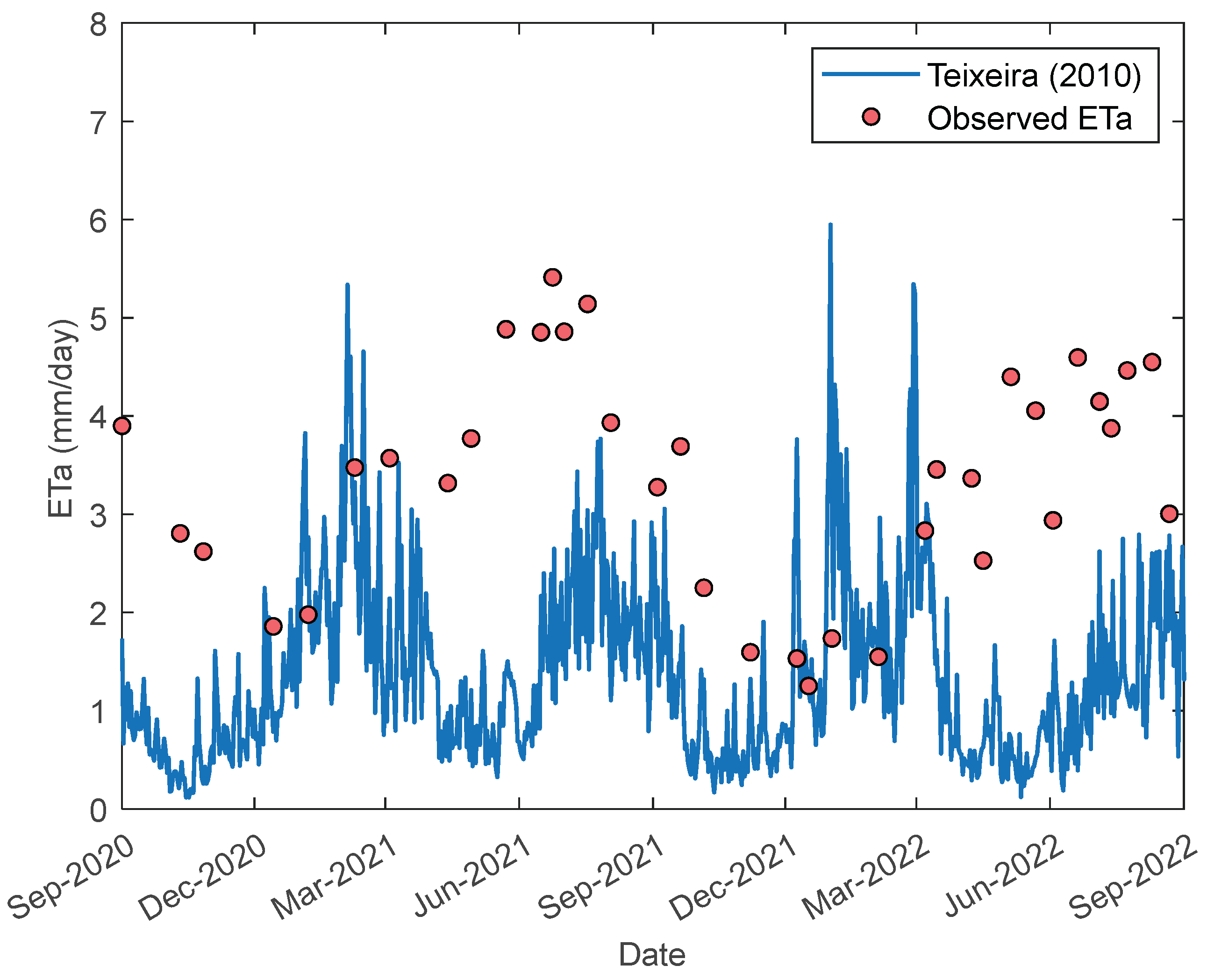
To highlight the importance of region-specific calibration, satellite-based ETa results obtained using the SAFER model coefficients proposed by Teixeira [
4] (a = 1.90 and b = 0.008) are presented in
Figure 4, compared against observed ETa values.
In
Figure 4, SAFER model results obtained using the coefficients proposed in the literature are shown with a continuous line, while satellite-based ETa observations are represented by discrete points. Examination of
Figure 4 indicates that there is no significant agreement between the observed values and the model outputs. The overall dataset yielded R² = 0.0139 and RMSE = 2.2201, clearly demonstrating the necessity of optimizing the SAFER model coefficients to represent the specific study area.
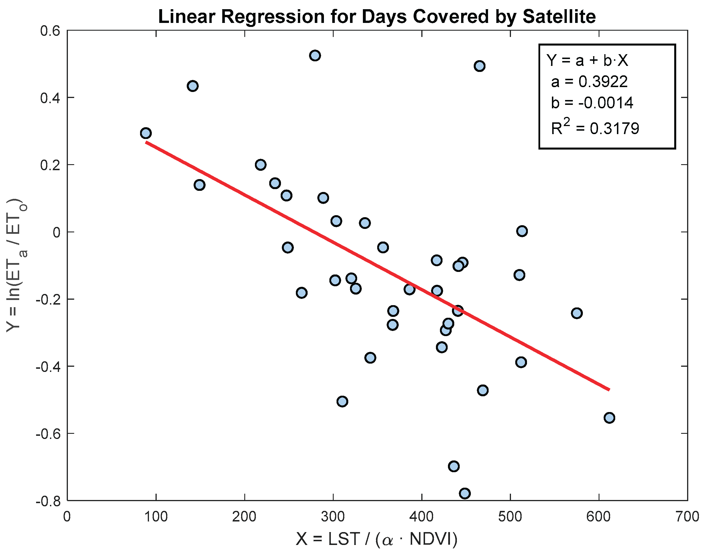
3.1.2. Model Calibration Using Linear Regression
The SAFER model, given by Equation (2), can be transformed into a linear form through variable transformations, X = LST / (αₛ ⋅ NDVI) and Y = ln(ETa / ETo), allowing the coefficients
a and
b to be easily determined via regression analysis. In the majority of studies in the literature, calibration has been performed using this procedure, and the resulting calibrated model outputs are presented in
Figure 5.
As shown in
Figure 5, the SAFER model coefficients obtained using this method are
a = 0.3922 and
b = 0.0014. However, as illustrated, traditional linear regression methods assign fixed parameters based on a single linear relationship, which limits the model’s generalizability under varying climatic and surface conditions. Moreover, the distribution of data points around the regression line covers a relatively wide range. Performance metrics obtained with this approach are R² = 0.3179, RMSE = 0.2409, and MAE = 0.1730, highlighting the necessity of determining
a and
b coefficients that accurately represent the characteristics of the study area.
As noted above, directly using parameters determined for other regions or cropping patterns may not be appropriate. In addition, linear regression-based calibration can fail to capture the nuanced behavior of parameters, motivating the development of a heuristic-based nonlinear modeling framework in this study.
3.1.3. Parameter Optimization via Simulation-Optimization
Derivative-based nonlinear optimization methods that could be used for this purpose are often sensitive to initial values and the search space, frequently becoming trapped in local minima and limiting their ability to reach global solutions [
38,
39]. To overcome these limitations, the SOS algorithm, capable of capturing all nonlinear dynamics of the SAFER model, requiring no algorithm-specific parameters, and balancing global and local search capabilities, was employed. This approach allows model parameters to reach their optimal values within the defined search space without additional calibration, with all model metrics and graphical outputs generated directly.
Furthermore, the flexible SOS-based framework is compatible with the integration of alternative heuristic algorithms. Using the proposed SOS-based model, the SAFER model parameters given in Equation (2) were determined as a = 0.314829 and b = -0.001216, and the performance of the SAFER S/O model was compared against other calibration methods reported in the literature using various error evaluation metrics.
As shown in the first row of
Table 2, when the SAFER model is applied using the coefficients provided in the original study (a = 1.90, b = -0.008), its performance is very low across all evaluation metrics. This clearly indicates that the SAFER model must be calibrated for the specific study area to produce reliable results.
In the second row of the table, the SAFER model is calibrated as shown in
Figure 5, and the performance of the model using the determined coefficients (a = 0.3922, b = -0.0014) is evaluated in terms of MSE, MAE, RMSE, MAPE, R², and NSE. The detailed results are presented in
Table 2.
The last row of
Table 2 presents the results obtained from the S/O-based SAFER model proposed in this study. As can be seen, the proposed S/O-SAFER model exhibits the best performance across all metrics. In all analyses presented in
Table 2, the Mean Squared Error (MSE) was selected as the objective function, following common practice in the literature.
To assess the effect of the objective function choice on model performance, the S/O-SAFER model was also evaluated using different optimization criteria. The objective functions considered included MSE, MAE, RMSE, MAPE, R², and NSE, and the resulting performances were compared across all metrics. The detailed results of these analyses are presented in
Table 3.
In
Table 3, the best values for each metric are highlighted in bold. Overall, changing the objective function does not appear to have a significant impact on model performance. However, to emphasize the overall reliability and performance of the model, it is appropriate to consider
R² and
NSE metrics alongside
MAE. To assess the influence of outliers,
RMSE or
MSE can be used as supplementary indicators, while
MAPE serves as a supportive metric to reveal the relative deviations of predictions. The lack of notable differences across all metrics indicates that the model behaves consistently across different performance criteria and exhibits low sensitivity to minor changes in parameter values.
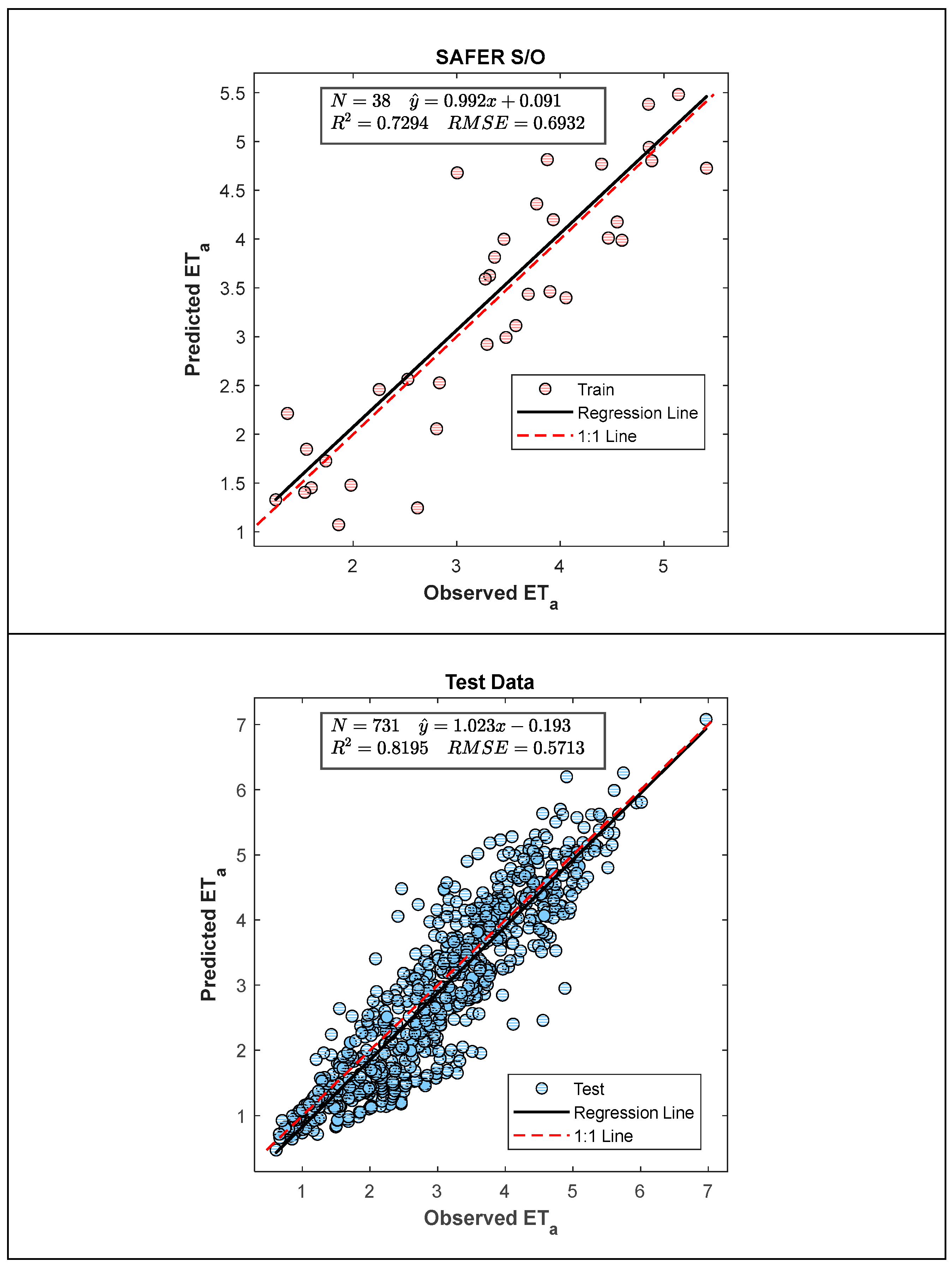
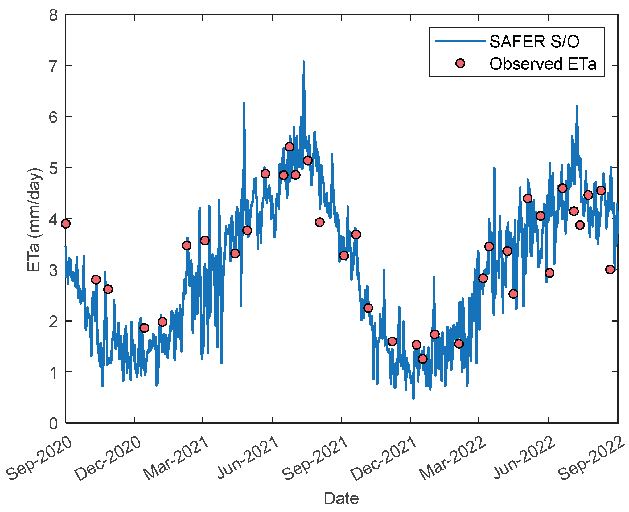
Scatter plots for the model’s training and testing phases are presented in
Figure 6, while the comparison between satellite observations and model results is shown in
Figure 7, providing a more intuitive visual representation of the outcomes.
As shown in
Figure 6, although only approximately 5% of the total dataset was used for training the model, the performance during testing was calculated as R² = 0.8195 and RMSE = 0.5713. Furthermore, the temporal variation plot presented in
Figure 7 demonstrates that the predicted ETa values are seasonally consistent with the observations and generally exhibit high prediction accuracy.
3.2. Application of the Proposed Relationships via Parameter Optimization
In the previous section, the SAFER model was evaluated using the coefficients provided in reference [
4], as well as the regression coefficients obtained via linear regression after logarithmic transformation (
Figure 5), alongside the proposed SAFER S/O approach. Analyses conducted using a and b coefficients determined for different objective functions showed that the SAFER S/O model consistently outperformed all alternative objective functions.
In this section, the proposed equations—LM-I, LM-II, NLM-I, and NLM-II—were implemented using the S/O model with MSE as the objective function. The coefficients obtained for each model are summarized in
Table 4.
The model performances obtained using the coefficients of the proposed equations, as summarized in
Table 4 and determined via the S/O model, are comparatively presented in
Table 5.
According to
Table 5, the proposed NLM-II model outperforms both the SAFER model and the proposed linear models across all error evaluation metrics.
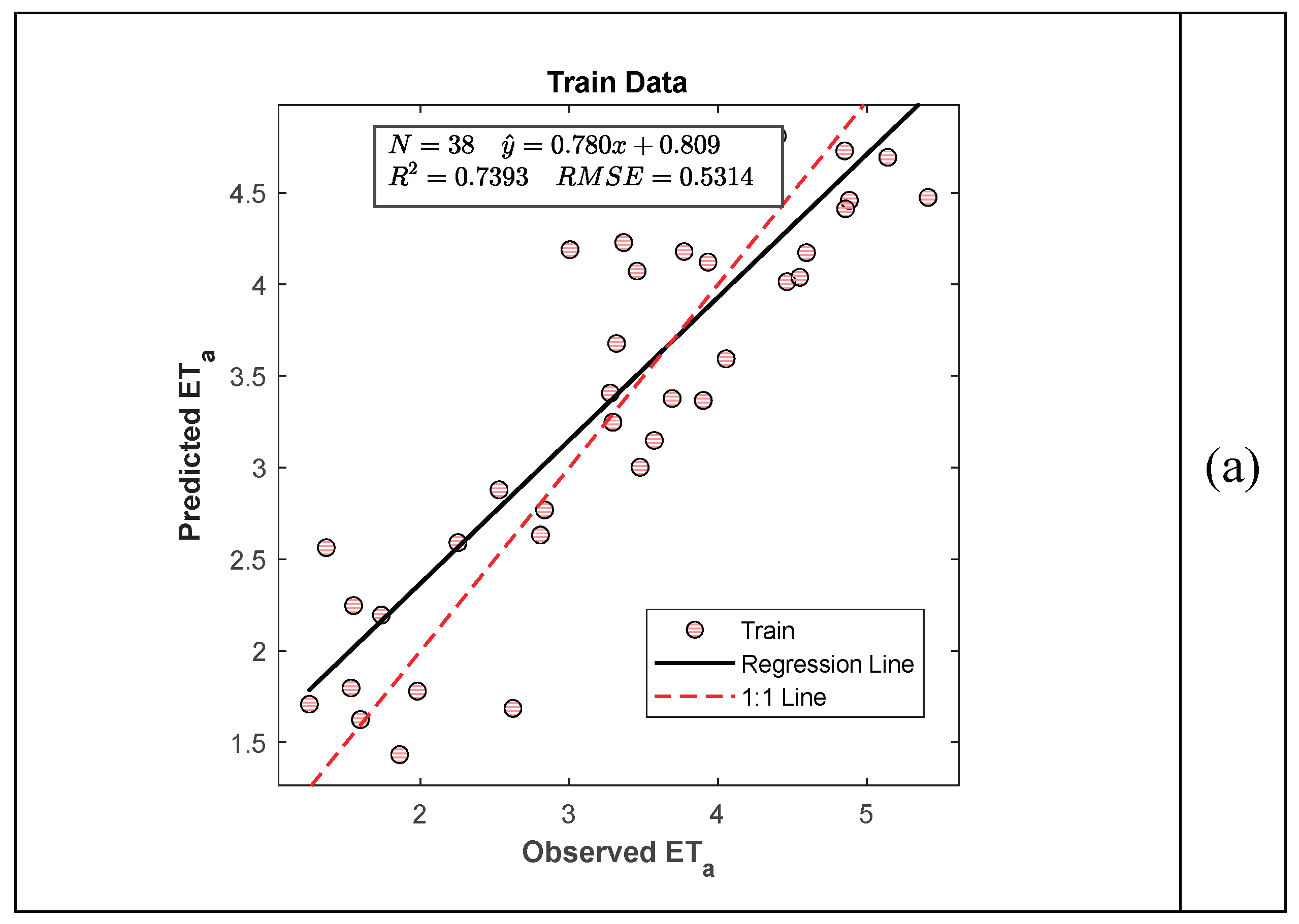
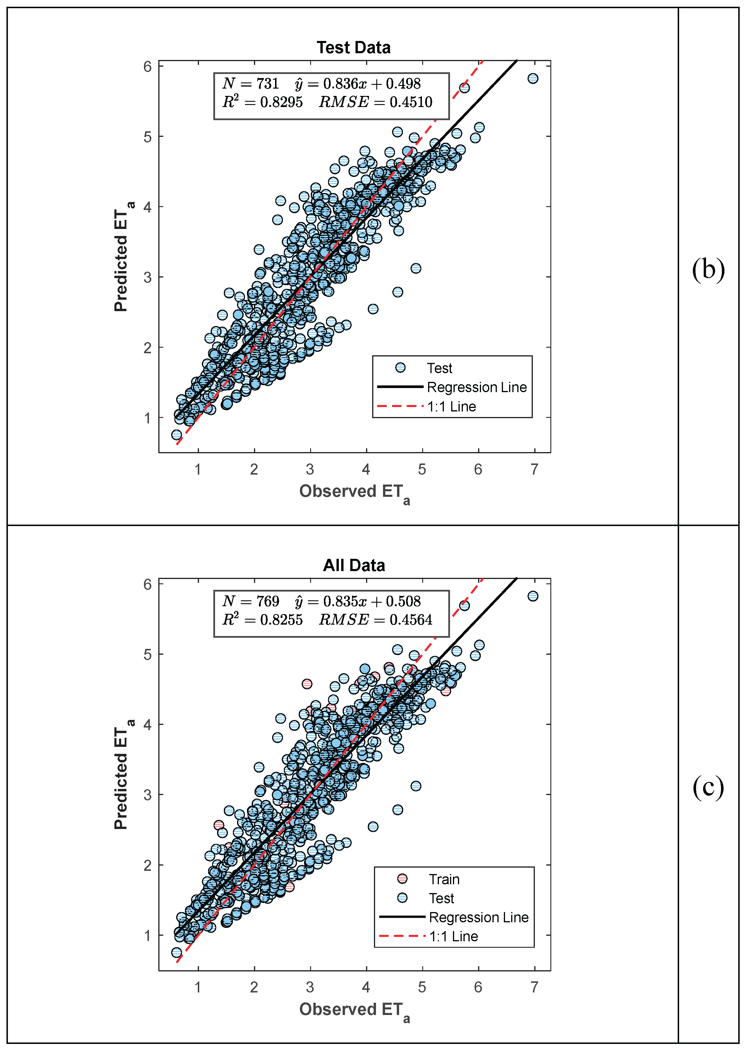
Scatter plots for the PLNM-II model, which demonstrates the highest performance among SAFER and the other four proposed formulations across all evaluation criteria, are presented in
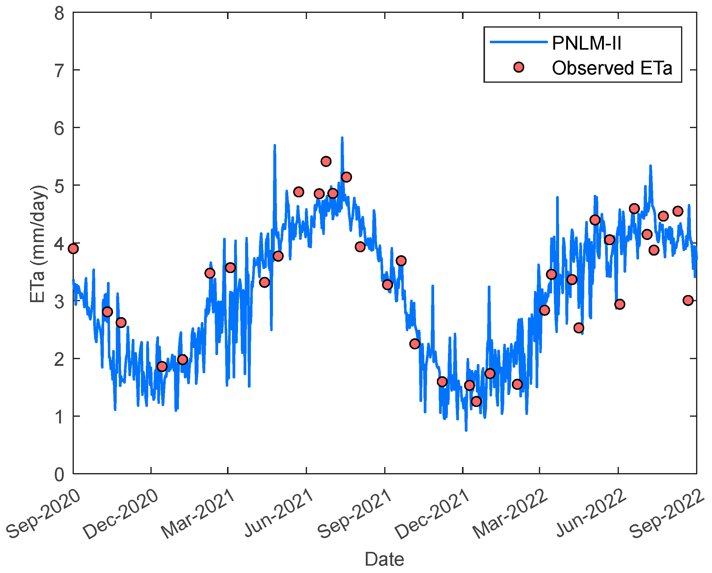
Figure 8 for the training, testing, and entire datasets. The comparative visualization of satellite observations and model predictions is shown in
Figure 9.
As shown in
Figure 9, although only approximately 5% of the total dataset was used for model training, the performance during testing was calculated as R² = 0.8295 and RMSE = 0.4913.
The performance of the SAFER S/O model (R² = 0.8195) is close to that of PNLM-II, whereas its RMSE (0.5713) is noticeably higher than that of PNLM-II (0.4913). Furthermore, the temporal variation plot presented in
Figure 9 demonstrates that the predicted ETa values are seasonally consistent with the observations and exhibit overall high prediction accuracy.
3.3. Soft Computing Approaches
Evapotranspiration (ET) prediction can become significantly challenging, especially for large-scale applications and in cases with limited meteorological data, when using conventional physical or empirical methods. Therefore, in recent years, soft computing approaches have gained prominence due to their data-driven flexible structures and capacity to learn nonlinear relationships. Within the scope of soft computing, artificial neural network (ANN)-based models have long been widely employed [
40,
41,
42].
In this study, the soft computing methods applied include Random Forest (RF), Bagged Trees (BT), Support Vector Machines (SVM), and Generalized Additive Model (GAM), and their performance was compared with the ANN model proposed by Karahan et al. (2024). RF is an ensemble algorithm that combines bootstrap sampling with a random subspace approach, allowing it to model nonlinear relationships among variables with high accuracy and enabling variable importance analysis [
43]. BT is an application of the classic bagging approach based on bootstrap sampling, where averaging a large number of decision trees enhances prediction stability [
44]. SVM is a kernel-based machine learning method capable of creating effective decision boundaries in high-dimensional data structures [
45]. GAM is a semi-parametric regression approach that flexibly models nonlinear relationships through smoothing functions (splines) [
46].
These black-box models evaluate energy–water balance variables (LST, NDVI, α, ETo) flexibly in ET prediction, capturing nonlinear interactions and providing highly accurate forecasts. In a similar study, Karahan et al. developed an ANN-based model, achieving R² values of 0.7547 and 0.7561 for test and full datasets, respectively, in daily ET prediction [
24]. While these results indicate satisfactory overall model performance, it was noted that the error increased for high ETa values. This suggests that ANN models require a larger training dataset to learn complex relationships, and the model trained with only approximately 5% of the total dataset could not achieve sufficient learning. The study reported performance improvements with an increased number of training samples.
In the present study, in addition to the SAFER model and the proposed linear and nonlinear formulations, different soft computing methods were applied using the same dataset, and the obtained results are summarized in
Table 6.
Examining
Table 6, it is observed that the best overall model performance in terms of MSE, RMSE, R², and NSE was achieved by the Bagged Trees (BT) method. In terms of MAE and MAPE, the Support Vector Machines (SVM) model performed the best. The highest performance values for each metric in the table are highlighted in bold. Although the Generalized Additive Model (GAM) exhibited very high performance during the training phase (R² = 0.9963), its test performance dropped to 0.7906. Overall, all models achieved acceptable performance levels, yielding results comparable to the ANN model.
4. Discussion
In this study, the linear (PLM-I and PLM-II) and nonlinear (PNLM-I and PNLM-II) formulations used for modeling ETa with remote sensing-based variables were comprehensively evaluated in terms of both their capacity to represent physical processes and their statistical performance metrics. Linear models explain the relationship between ETa and variables such as LST, NDVI, αₛ, and ETo using fixed coefficients, whereas nonlinear models offer a more flexible approach that acknowledges that ET processes are often scalable, proportional, and frequently exponential in nature. Consequently, considering the physical mechanisms, nonlinear models have a greater ability to capture the complex seasonal behaviors of ETa.
Examining the linear models, LST generally shows a negative effect, NDVI and αₛ show positive effects, and ETo is the dominant determinant. However, the linear form assumes that these effects remain constant over time, which limits the model’s representativeness, especially during dry seasons when plant–atmosphere interactions intensify. The results in
Table 5 confirm this limitation: although the best-performing linear model, LM-II, achieved R² = 0.8227 and NSE = 0.8226 on the test dataset, it still exhibits limited flexibility in capturing the full range of seasonal dynamics compared to nonlinear models.
Nonlinear models, on the other hand, provide a structure more consistent with the physical nature of ETa. In PNLM-I and PNLM-II, the exponential dominance of ETo appropriately reflects the controlling role of atmospheric demand on ETa. The positive exponential effects of NDVI and αₛ represent the contribution of vegetation and surface properties to evapotranspiration processes in a scaled manner, while including LST in the denominator correctly accounts for the inhibitory effect of increased surface temperatures on ETa during dry periods. In particular, the PNLM-II model’s performance on the test dataset (R² = 0.8295, RMSE = 0.4913) clearly demonstrates that the model accurately represents both the data structure and the water–energy interactions at the appropriate scale.
The exponential form of the SAFER model clearly illustrates the sensitivity of ETa to its controlling variables:
Even small variations in the parameters produce substantial changes in the outputs, mathematically characterizing the high sensitivity of the model.
The coefficients suggested by Teixeira (2010) [
4] produced high error values (RMSE ≈ 2.30), reflecting the exponential sensitivity of the model. Following calibration via linear regression, the RMSE decreased to 0.59, highlighting the substantial impact of small parameter adjustments on model performance.
One of the most notable findings of this study is that the proposed nonlinear model, PNLM-II, not only outperformed the linear models but also surpassed all soft computing approaches on the test set. In the literature, flexible data-driven methods such as RF, BT, SVM, and GAM are generally considered to provide higher accuracy than nonlinear functional models. However, due to the limited training data used in this study, the opposite was observed:
Among the soft computing methods, the best-performing model, BT, achieved R² = 0.8137 and RMSE = 0.5084 on the test set, whereas the PNLM-II model achieved higher accuracy with R² = 0.8295 and lower RMSE = 0.4913.
The superior performance of PNLM-II over soft computing approaches can be attributed to its strong integration of physical processes, compact structure, and controlled representation of nonlinear interactions.
Specifically, PNLM-II analytically incorporates the water–energy balance components that govern ETa, making the model more stable and physically consistent than black-box approaches. Moreover, unlike methods such as RF, BT, and GAM, which rely on numerous parameters and are prone to overfitting when data are limited, PNLM-II’s parsimonious structure ensures balanced performance across both training and test sets. In addition, while soft computing algorithms learn relationships freely, PNLM-II provides a physically guided and controlled nonlinear representation, which offers clear advantages during dry seasons and under high ET conditions. Although SAFER-derived models are generally known to perform well during wet periods but less effectively in dry periods [
23], in this study, both the SAFER S/O and the proposed PNLM models produced results that were consistent with observations even during dry periods, as demonstrated by the time series analysis in
Figure 7. This outcome highlights the models’ strong physical consistency and the effectiveness of their nonlinear formulations.In conclusion, while linear models are useful for interpreting the direction and magnitude of variable effects, this study clearly demonstrates that nonlinear models—particularly PNLM-II—provide more realistic representation of physical processes and achieve the highest accuracy and seasonal consistency. Although soft computing methods offer high predictive accuracy, PNLM-II’s ability to outperform them on the test set indicates that well-defined, physically and analytically based models can be more effective than machine learning approaches when properly formulated.
5. Conclusions
In this study, two linear (LM-I, LM-II) and two nonlinear (NLM-I, NLM-II) formulations were developed to model evapotranspiration (ETa) using remote sensing-based variables, while SAFER model parameters were recalibrated via an S/O optimization approach, resulting in parametric models that are both physically representative and flexible. Model performances were comprehensively evaluated against common soft computing methods (RF, BT, SVM, and GAM) as well as the ANN model from the literature. Due to reliance on Landsat-8 overpass days, the training dataset was inherently sparse (approximately one observation every 16 days), limiting the learning capacity of high-parameter AI models; nevertheless, the proposed parametric models, with their more compact structures, achieved high-accuracy predictions even under low data density. The results indicate that nonlinear formulations are more consistent with the physical nature of ETa and better capture the data distribution than linear models, as their scalability and flexibility are reflected in improved accuracy. Considering all evaluation metrics (MSE, RMSE, MAE, MAPE, R², NSE), the NLM-II model demonstrated the highest performance among both linear–nonlinear formulations and all soft computing methods, maintaining low error levels even during periods of seasonal variation and high ETa, making it a robust option for operational ETa estimation.
Although soft computing methods can perform strongly with large datasets, their performance in this study was limited by the small training dataset, allowing parametric approaches to outperform them. Overall, this study demonstrates that linear and nonlinear ETa models can be effectively employed with remote sensing data, parametric optimization via the SAFER S/O approach significantly enhances model performance, the nonlinear NLM-II model achieves the highest accuracy across all evaluation metrics, soft computing methods under sparse data conditions are outperformed by parametric models, and compact, physically representative models offer clear advantages for sparse Landsat-based datasets. The proposed nonlinear formulations successfully capture the complex and seasonally dependent dynamics of ETa, with the NLM-II model emerging as an effective and practical solution for operational applications and large-scale ET estimation.
Data Availability Statement
The data that support the findings of this study are available from the author upon reasonable request.
Acknowledgments
The author gratefully acknowledges the support of the Scientific and Technological Research Council of Turkey (TUBITAK) for project no. 122Y007, which provided the data used in this study.
Conflicts of Interest
The author declares no conflict of interest.
Abbreviations
The following abbreviations are used in this manuscript:
| S/O |
Simulation/Optimization |
| SAFER |
Simplified Approach for Evapotranspiration Retrieval |
| ETo |
Reference Evapotranspiration |
| ETa |
Actual Evapotranspiration |
| ETf |
Evapotranspiration Fraction (ETa/ETo) |
| LST |
Land Surface Temperature |
| NDVI |
Normalized Difference Vegetation Index |
| α (alpha) |
Surface Albedo Coefficient |
| SEBAL |
Surface Energy Balance Algorithm for Land |
| METRIC |
Mapping Evapotranspiration at High Resolution |
| SSEB |
Simplified Surface Energy Balance |
| MODIS |
Moderate Resolution Imaging Spectroradiometer |
| NM |
Nelder–Mead Optimization Algorithm |
| BFGS |
Broyden–Fletcher–Goldfarb–Shanno Optimization Algorithm |
| MSE |
Mean Squared Error |
| MAE |
Mean Absolute Error |
| RMSE |
Root Mean Squared Error |
| R² |
Coefficient of Determination |
References
- Bastiaanssen, W. G., Pelgrum, H., Wang, J., Ma, Y., Moreno, J. F., Roerink, G. J., & Van der Wal, T. (1998). A remote sensing surface energy balance algorithm for land (SEBAL).: Part 2: Validation. Journal of hydrology, 212, 213-229. [CrossRef]
- Allen, R. G., Tasumi, M., & Trezza, R. (2007). Satellite-based energy balance for mapping evapotranspiration with internalized calibration (METRIC)—Model. Journal of irrigation and drainage engineering, 133(4), 380-394. [CrossRef]
- Senay, G. B., Bohms, S., Singh, R. K., Gowda, P. H., Velpuri, N. M., Alemu, H., & Verdin, J. P. (2013). Operational evapotranspiration mapping using remote sensing and weather datasets: A new parameterization for the SSEB approach. JAWRA Journal of the American Water Resources Association, 49(3), 577-591. [CrossRef]
- Teixeira, A. H. D. C. (2010). Determining regional actual evapotranspiration of irrigated crops and natural vegetation in the São Francisco river basin (Brazil) using remote sensing and Penman-Monteith equation. Remote Sensing, 2(5), 1287-1319. [CrossRef]
- Roerink, G. J., Su, Z., & Menenti, M. (2000). S-SEBI: A simple remote sensing algorithm to estimate the surface energy balance. Physics and Chemistry of the Earth, Part B: Hydrology, Oceans and Atmosphere, 25(2), 147-157. [CrossRef]
- Venancio, L. P., Mantovani, E. C., Amaral, C. H. D., Neale, C. M. U., Filgueiras, R., Gonçalves, I. Z., & Cunha, F. F. D. (2020). Evapotranspiration mapping of commercial corn fields in Brazil using SAFER algorithm. Scientia Agricola, 78(4), e20190261. [CrossRef]
- Coaguila, D. N., Hernandez, F. B., Teixeira, A. H. D. C., Franco, R. A., & Leivas, J. F. (2017). Water productivity using SAFER-Simple Algorithm for Evapotranspiration Retrieving in watershed. Revista Brasileira de Engenharia Agrícola e Ambiental, 21(8), 524-529. [CrossRef]
- Teixeira, A. D. C., Bastiaanssen, W. G., Ahmad, M., & Bos, M. G. (2009). Reviewing SEBAL input parameters for assessing evapotranspiration and water productivity for the Low-Middle São Francisco River basin, Brazil: Part A: Calibration and validation. Agricultural and forest meteorology, 149(3-4), 462-476. [CrossRef]
- Teixeira, A. D. C., Hernandez, F. B. T., Lopes, H. L., Scherer-Warren, M., Bassoi, L. H., LOPES, H. L., ... & BASSOI, L. H. (2014). A comparative study of techniques for modeling the spatiotemporal distribution of heat and moisture fluxes at different agroecosystems in Brazil.
- Ritchie, J. T. (1972). Model for predicting evaporation from a row crop with incomplete cover. Water resources research, 8(5), 1204-1213. [CrossRef]
- Hargreaves, G. H., & Samani, Z. A. (1985). Reference crop evapotranspiration from temperature. Applied engineering in agriculture, 1(2), 96-99. [CrossRef]
- Stroosnijder, L. (1987). Soil evaporation: test of a practical approach under semi-arid conditions. Netherlands Journal of Agricultural Science, 35(3), 417-426. [CrossRef]
- Gallardo, M., Snyder, R. L., Schulbach, K., & Jackson, L. E. (1996). Crop growth and water use model for lettuce. Journal of irrigation and drainage engineering, 122(6), 354-359. [CrossRef]
- Pereira, L. S., Allen, R. G., Smith, M., & Raes, D. (2015). Crop evapotranspiration estimation with FAO56: Past and future. Agricultural water management, 147, 4-20. [CrossRef]
- Anagnostolpoulou, C., Tolika, K., Skoulikaris, C., & Zafirakou, A. (2016). Climate change assessments over a Greek catchment using RCM’s projection. In Perspectives on atmospheric sciences (pp. 655-661). Cham: Springer International Publishing.
- Souza, J. M. F., Alves Júnior, J., Casaroli, D., Evangelista, A. W. P., & Mesquita, M. (2020). Validation of safer algorithm to estimate sugarcane crop evapotranspiration.
- Teixeira, A. H. D. C., Leivas, J. F., Hernandez, F. B. T., & Franco, R. A. M. (2017). Large-scale radiation and energy balances with Landsat 8 images and agrometeorological data in the Brazilian semiarid region. Journal of Applied Remote Sensing, 11(1), 016030-016030. [CrossRef]
- Nadeem, A. A., Zha, Y., Shi, L., Zafar, Z., Ali, S., Zhang, Y., ... & Zubair, M. (2023). SAFER-ET based assessment of irrigation patterns and impacts on groundwater use in the central Punjab, Pakistan. Agricultural Water Management, 289, 108545. [CrossRef]
- do Nascimento Leão, F. D. A., Mercante, E., Oliveira, W. K. M., Boas, M. A. V., Correa, M. M., Bazzi, C. L., & da Silva Jr, A. C. (2025). Determination of evapotranspiration for citrus using SAFER algorithm in the Oriental Amazon. Remote Sensing Applications: Society and Environment, 38, 101526.
- Venancio, L. P., Mantovani, E. C., Amaral, C. H. D., Neale, C. M. U., Filgueiras, R., Gonçalves, I. Z., & Cunha, F. F. D. (2020). Evapotranspiration mapping of commercial corn fields in Brazil using SAFER algorithm. Scientia Agricola, 78(4), e20190261. [CrossRef]
- Teixeira, A. D. C. (2012). Modelling evapotranspiration by remote sensing parameters and agro-meteorological stations. Remote Sensing and Hydrology, 352, 154-157.
- de C. Teixeira, A. H., Scherer-Warren, M., Hernandez, F. B., Andrade, R. G., & Leivas, J. F. (2013). Large-scale water productivity assessments with MODIS images in a changing semi-arid environment: a Brazilian case study. Remote Sensing, 5(11), 5783-5804. [CrossRef]
- Salamanca Lopez, K. A., João, G. A., Acioli Imbuzeiro, H. M., Vanella, D., Consoli, S., Longo Minnolo, G., ... & Oliveira-Júnior, J. F. D. (2025). Evaluating a Simple Algorithm for an Evapotranspiration Retrieval Energy Balance Model in Mediterranean Citrus Orchards. Water, 17(22), 3286. [CrossRef]
- Karahan, H., Cetin, M., Can, M. E., & Alsenjar, O. (2024). Developing a new ANN model to estimate daily actual evapotranspiration using limited climatic data and remote sensing techniques for sustainable water management. Sustainability, 16(6), 2481. [CrossRef]
- Cetin, M., Alsenjar, O., Aksu, H., Golpinar, M. S., & Akgul, M. A. (2023). Comparing actual evapotranspiration estimations by METRIC to in-situ water balance measurements over an irrigated field in Turkey. Hydrological Sciences Journal, 68(8), 1162-1183. [CrossRef]
- Karahan, H., Çetin, M., Can, M. E., & Gültekin, U. (2025). TÜBİTAK (122Y007), Final Report, Ankara, Turkey.
- Allen, R. G., Pereira, L. S., Raes, D., & Smith, M. (1998). Crop evapotranspiration-Guidelines for computing crop water requirements-FAO Irrigation and drainage paper 56. Fao, Rome, 300(9), D05109.
- Tasumi, M., Allen, R. G., & Trezza, R. (2008). At-surface reflectance and albedo from satellite for operational calculation of land surface energy balance. Journal of hydrologic engineering, 13(2), 51-63. [CrossRef]
- Didan, K. (2015). MOD13Q1 MODIS/Terra vegetation indices 16-day L3 global 250m SIN grid V006. NASA EOSDIS Land Processes Distributed Active Archive Center (DAAC) data set, MOD13Q1-006.
- Wan, Z., Hook, S., & Hulley, G. (2015). MYD11A1 MODIS/aqua land surface temperature/emissivity daily L3 global 1km SIN grid V006. NASA EOSDIS Land Processes Distributed Active Archive Center (DAAC) data set, MYD11A1-006.
- Gorelick, N., Hancher, M., Dixon, M., Ilyushchenko, S., Thau, D., & Moore, R. (2017). Google Earth Engine: Planetary-scale geospatial analysis for everyone. Remote sensing of Environment, 202, 18-27. [CrossRef]
- de Castro Teixeira, A. H., Bastiaanssen, W. G., Ahmad, M. U. D., Moura, M. D., & Bos, M. G. (2008). Analysis of energy fluxes and vegetation-atmosphere parameters in irrigated and natural ecosystems of semi-arid Brazil. Journal of Hydrology, 362(1-2), 110-127. [CrossRef]
- Safre, A. L., Nassar, A., Torres-Rua, A., Aboutalebi, M., Saad, J. C., Manzione, R. L., ... & Anderson, M. C. (2022). Performance of Sentinel-2 SAFER ET model for daily and seasonal estimation of grapevine water consumption. Irrigation Science, 40(4), 635-654. [CrossRef]
- Teixeira, A., Leivas, J., Takemura, C., Garçon, E., Sousa, I., & Azevedo, A. (2024). Monitoring anomalies on large-scale energy and water balance components by coupling remote sensing parameters and gridded weather data. International Journal of Biometeorology, 68(12), 2597-2612. [CrossRef]
- Cheng, M. Y., & Prayogo, D. (2014). Symbiotic organisms search: a new metaheuristic optimization algorithm. Computers & Structures, 139, 98-112. [CrossRef]
- Khalifeh, S., Esmaili, K., Khodashenas, S. R., & Khalifeh, V. (2020). Estimation of nonlinear parameters of the type 5 Muskingum model using SOS algorithm. MethodsX, 7, 101040. [CrossRef]
- Rezaei-Estakhroueiyeh, A., Jalalkamali, N., & Momeniroghabadi, M. (2020). Data on optimal operation of Safarud Reservoir using symbiotic organisms search (SOS) algorithm. Data in brief, 29, 105327. [CrossRef]
- Karahan, H. (2013). Discussion of “parameter estimation of nonlinear Muskingum models using Nelder-Mead simplex algorithm” by Reza Barati. Journal of Hydrologic Engineering, 18(3), 365-367. [CrossRef]
- Karahan, H. (2014). Discussion of “improved nonlinear Muskingum model with variable exponent parameter” by said M. Easa. Journal of Hydrologic Engineering, 19(10), 07014007.
- Haykin, S., Nie, J., & Currie, B. (1999). Neural network-based receiver for wireless communications. Electronics Letters, 35(3), 203–205. [CrossRef]
- Karahan, H., & Ayvaz, M. T. (2006). Forecasting aquifer parameters using artificial neural networks. Journal of Porous Media, 9(5). [CrossRef]
- Pal, M., & Mather, P. M. (2003). An assessment of the effectiveness of decision tree methods for land cover classification. Remote Sensing of Environment, 86(4), 554–565. [CrossRef]
- Breiman, L. (2001). Random forests. Machine Learning, 45(1), 5–32.
- Breiman, L. (1996). Bagging predictors. Machine Learning, 24(2), 123–140.
- Cortes, C., & Vapnik, V. (1995). Support-vector networks. Machine Learning, 20(3), 273–297.
- Xiang, D. (2001). Fitting generalized additive models with the GAM procedure. In SUGI Proceedings (pp. 256–326). Cary, NC: SAS Institute, Inc.
|
Disclaimer/Publisher’s Note: The statements, opinions and data contained in all publications are solely those of the individual author(s) and contributor(s) and not of MDPI and/or the editor(s). MDPI and/or the editor(s) disclaim responsibility for any injury to people or property resulting from any ideas, methods, instructions or products referred to in the content. |
© 2026 by the authors. Licensee MDPI, Basel, Switzerland. This article is an open access article distributed under the terms and conditions of the Creative Commons Attribution (CC BY) license (http://creativecommons.org/licenses/by/4.0/).