Prediction of Potential Evapotranspiration via Machine Learning and Deep Learning for the Murat River Basin

1. Introduction

Evapotranspiration (ET) describes the process through which moisture is returned from the earth’s surface to the atmosphere by combining evaporation from the land and transpiration from plants [1]. In hydrological research, potential evapotranspiration (PET) is widely regarded as a key parameter, essential for validating and refining rainfall-runoff models and broader hydrological cycle assessments, as well as enhancing climate and meteorological forecasting models [2,3]. However, existing PET models often depend on a range of input variables such as temperature, precipitation, solar radiation, wind speed, and humidity posing challenges when data are sparse or inaccessible [4,5,6,7]. This study aims to address these limitations by predicting PET in the Murat River Basin, located in southeast Turkey, using a temperature-only approach. Employing monthly temperature data from the past four decades (1979–2021), we apply the Thornthwaite equation, which requires only temperature and latitude as inputs, making it highly suitable for data-limited environments.

The Murat River Basin is located in the southeastern part of Turkey which is characterized by a Mediterranean climate, where agricultural water demand is largely driven by ET during the dry season, necessitating extensive irrigation practices in open fields. This challenge is common in semi-arid regions, where limited rainfall necessitates efficient irrigation practices, making accurate PET estimation vital for agricultural planning [4]. The Thornthwaite model has demonstrated robust applicability for PET estimation and aridity assessments across various climatic contexts [8], offering a practical, accessible approach for environments with limited meteorological data.

In response to the predicted impacts of climate change, particularly the Clausius–Clapeyron relationship which suggests that rising temperature due to climate change will increase atmospheric moisture and intensify the hydrological cycle [9], thus, increasing temperature will enhance the exchange of water vapor between terrestrial ecosystems and the atmosphere. This study explores how PET might respond to these shifts. According to Bouchet’s complementary hypothesis, increased air temperatures could heighten atmospheric evaporative demand, potentially reducing PET rates under specific conditions [10]. Temperature-based PET estimation remains a widely applied and efficient technique in climatology and hydrology, providing an effective means of large-scale modeling [11]. PET plays a crucial role in meteorological research, highlighting the need for reliable measurement methods with guaranteed accuracy in hydrology and agricultural studies [12]. This study presents a novel PET prediction methodology utilizing Python libraries alongside machine learning and deep learning techniques. Machine learning, in particular, has emerged as an effective tool for forecasting time-series data, such as evapotranspiration (ET), independent of prior knowledge of underlying physical processes [3].

There are various methods used to estimate PET in various parts of the world. However, it is a challenge to select a suitable method for PET calculation, because the selection of an appropriate method for certain areas highly depends on data availability [6,7]. As a result of the lack of the required input data in the interested region of study, a key focus of this study is integrating machine learning (ML) and deep learning (DL) methodologies to improve PET predictions. Machine learning models, such as the support vector machine (SVM) [13,14], artificial neural network (ANN) [15], and random forest (RF), have shown promise in enhancing the precision of hydrological forecasting by incorporating complex environmental variables [13,16,17,18]. SVM, in particular, has demonstrated superior performance in predicting indices like the Standardized Precipitation Index (SPI) when provided with inputs such as wind speed and humidity [15]. Recently, the random forest (RF) method has become more popular because of its robustness and accuracy as a prediction algorithm, despite its simplicity [17,18]. According to Jing et al. (2019), SVM performs optimally when provided with wind speed, rainfall, and relative humidity as inputs. Indeed, deep learning-based models have a remarkable ability to predict future evapotranspiration [16]. Deep learning, through convolutional neural networks (CNNs) and other architectures, has also been successfully applied to time-series data, including ET, yielding accurate forecasts in diverse climates [16,19,20].

Despite these advancements, existing PET models frequently lack the flexibility to adapt to varying climatic conditions and often overlook uncertainty factors [19]. This study addresses these gaps by implementing rigorous model validation techniques and uncertainty analyses, providing a robust framework for PET prediction under different climate scenarios. Additionally, we compare traditional approaches with machine learning algorithms to highlight the practical implications of using novel ML and deep learning models in hydrological modeling, particularly its potential for enhancing PET predictions in data-scarce environments. The findings aim to contribute a data-efficient PET prediction methodology, providing a useful tool for regional water management and agricultural planning. This study’s novel approach not only improves upon traditional PET estimation by leveraging artificial intelligence but also seeks to establish a framework that can be adapted to other data-limited regions with similar hydrological needs.

2. Materials and Data Description

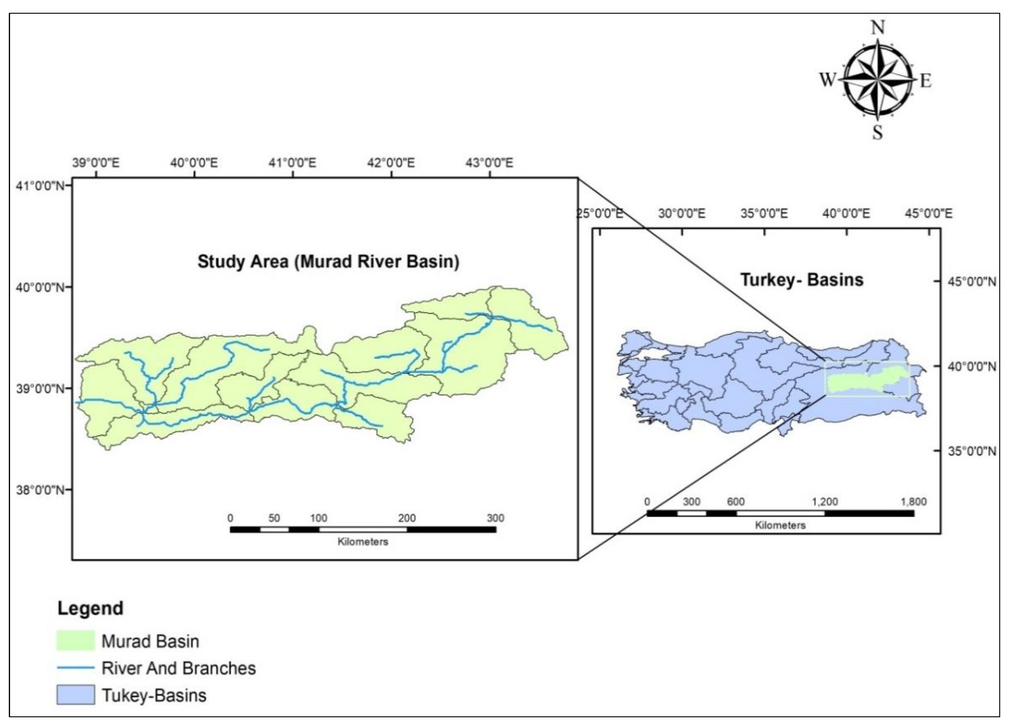
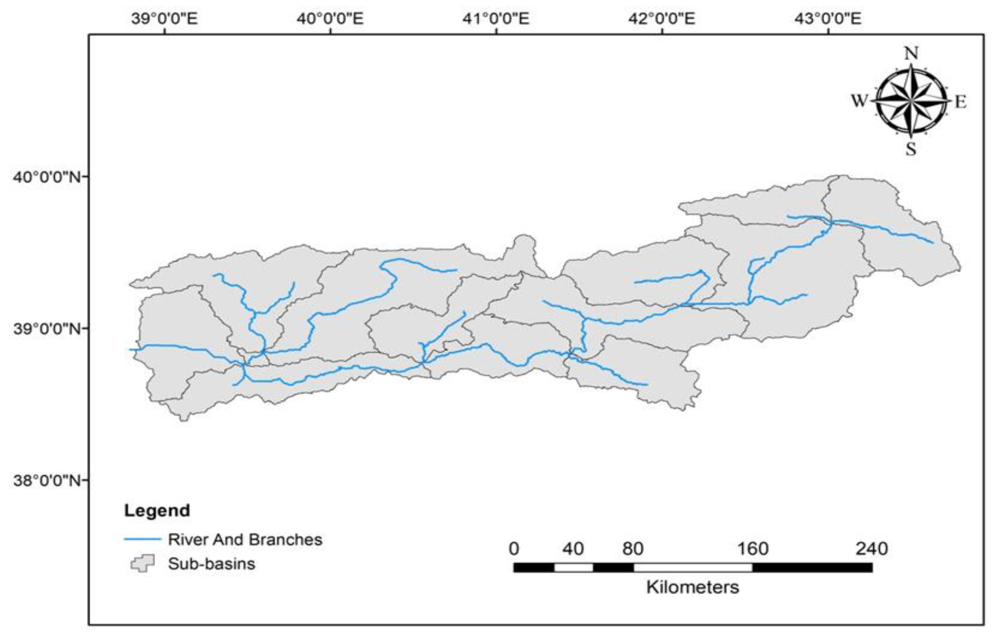
2.1. Study Area

The study area is the Murat River Basin in southeastern Turkey, as shown in Figure 1. The Murat River Basin is one of the principal origins of the Euphrates River, which traverses Turkey, Syria, and Iraq in an expansive journey. The latitude and the longitude ranges of the Murat River Basin are 40°04–40°02N and 38°53’–43°46’E, respectively.

The Murat River Basin is characterized by warm–dry summers and cold–wet winters. Precipitation is concentrated during the winter season, from November to April, and the total annual precipitation ranges from 350 to 1010 mm from location to location [21].

2.2. Data Collection

Data collection methods can differ from one country to another, depending on the specific research objectives, data types, units of measurement, and quantity required [22].

In this study, the data include a 12 m × 12 m digital elevation model (DEM) sourced from the US Geological Survey (USGS). Mean monthly temperature is the only climate data used for this study. The data were collected between 1979 and 2021 from 28 meteorological stations around the area, inside and outside the Murat River Basin. Table 1 lists the meteorological stations with their coordinates and serial numbers. This dataset is sufficient for conducting a comprehensive analysis and evaluation within this research area.

3. Methodology

3.1. Geographic Information System (GIS) Spatial Analysis and Modeling Setup

This study geographically analyzes and models the Murat River Basin, with a primary focus on predicting PET. The analysis begins by utilizing ArcGIS software to extract a high-resolution DEM with a spatial resolution of 12 m × 12 m. This detailed DEM allows for an accurate calculation of the basin’s total area, which is approximately 40,000 km². Understanding the basin’s dimensions and topography is essential for effective hydrological modeling and predicting PET, as these factors significantly influence water movement and availability within the region.

Thirteen distinct sub-basins were delineated through a comprehensive investigation of various hydrological processes, including filling, flow direction, flow accumulation, stream order, stream link, and basin analysis using GIS. This systematic approach enhances our understanding of the hydrological characteristics of the Murat River Basin, as illustrated in Figure 2. By identifying these sub-basins, we can better assess the spatial variability of hydrological phenomena, which is critical for accurate predictions of PET and effective water resource management in the region.

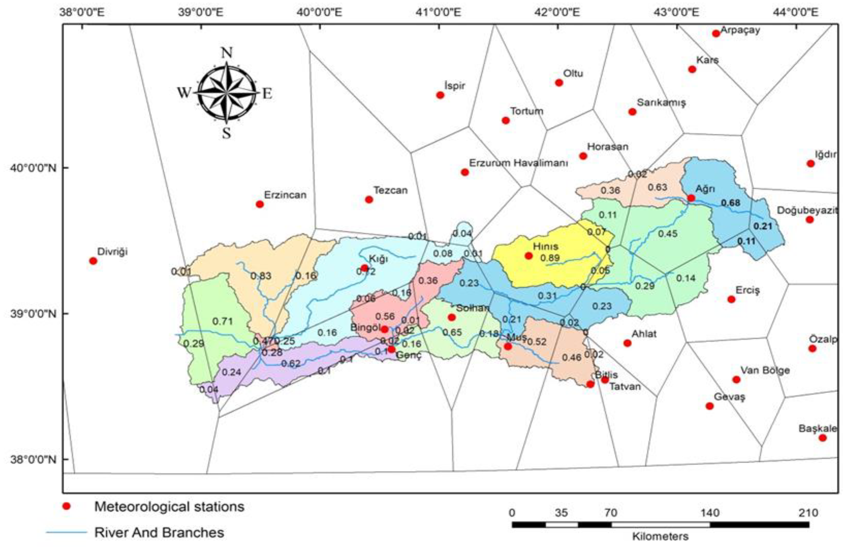
3.2. Interpolation Process Using the Thiessen Polygon Method

We employed the Thiessen polygon method for spatial interpolation in ArcGIS, creating polygons around each meteorological station based on its proximity to neighboring stations. This technique allows for a spatial representation of the catchment zones within the basin. The method operates under the assumption that the temperature recorded at each meteorological station serves as the best estimate for that station’s surrounding area compared to any other station’s measurements [23]. This approach is particularly useful for capturing the spatial variability of temperature across the Murat River Basin, which is essential for accurate predictions of PET and for understanding the region’s hydrological dynamics.

Figure 3 illustrates that meteorological data were collected over at least 40 years from 28 stations located both within and outside the research area. The geographical coordinates of these stations were integrated into the DEM to determine their relative distances and influence on the nearest sub-basins. Spatial interpolation methods are widely utilized to estimate meteorological data values in areas lacking direct measurements [24].

In this analysis, a weighted temperature value was computed for each station, calculated as the area influenced by the station divided by the total area of the respective sub-basin. This method allows us to assess the temperature contribution of individual stations within each sub-basin, as detailed in Table 2. The resulting data are then integrated to estimate temperature variations across the entire sub-basin, providing a comprehensive understanding of the thermal dynamics within the Murat River Basin.

3.3. Computing Potential Evapotranspiration (PET)

The Thornthwaite equation is used to calculate potential evapotranspiration (PET) based on temperature and latitude [25]. It can be expressed mathematically as follows:

$${\mathrm{E}}_{\mathrm{T}}=1.6{\mathrm{L}}_{\mathrm{a}}[{\displaystyle \frac{10\overline{\mathrm{T}}}{{\mathrm{I}}_{\mathrm{t}}}}{]}^{\mathrm{a}},$$

(1)

where, ${\mathrm{E}}_{\mathrm{T}}$ is monthly PET (cm); ${\mathrm{L}}_{\mathrm{a}}$is adjustment for the number of daylight hours and days in the month (depending on latitude; $\overline{\mathrm{T}}$ denotes mean monthly air temperature (C°); ${\mathrm{I}}_{\mathrm{t}}$ presents the total 12m monthly values of the heat index, i

$$i={\sum }_1^{12}i$$

(2)

$$\mathrm{and} \mathrm{i}={\left({\displaystyle \frac{\overline{T}}{5}}\right)}^{1.514}$$

(3)

a is empirical constant, where

$$\mathrm{a}=6.75 x10{-}^7 ({\mathrm{I}}_{\mathrm{t}}{)}^3 \text{–} 7.71 x10{-}^5 ({\mathrm{I}}_{\mathrm{t}}{)}^2+1.792 x{10}^{-2}\left({\mathrm{I}}_{\mathrm{t}}\right)+0.49239.$$

(4)

The Thornthwaite equation was implemented using RStudio to calculate PET. Additionally, standardized precipitation evapotranspiration index (SPEI) values for a long-term series related to the Murat River Basin were generated using R. The Thornthwaite equation calculated the monthly PET. The temperature-derived data were then used to calculate various PET timeframes [26].

3.4. Machine Learning and Deep Learning

In recent years, machine learning and deep learning techniques have significantly advanced the field of climate data analysis and prediction [27]. After computing the potential evapotranspiration (PET) for the past 42 years using temperature data and the Thornthwaite equation, three different machine learning models will be employed to predict PET for the succeeding 42 years. These models will utilize historical temperature data and PET values to identify patterns and relationships that can be applied to future projections. The selected machine learning and deep learning algorithms will be chosen for their capacity to capture non-linear patterns, temporal dependencies, and complex interactions between temperature and PET. By applying these advanced techniques, this study aims to generate more accurate and reliable forecasts of PET, providing valuable insights into potential future changes in evapotranspiration patterns. The outcomes of these predictions will be essential for understanding long-term evapotranspiration trends and their impact on regional hydrological processes and water resource management. This section explores the utilization of SVM, RF, and CNN to predict PET using temperature data spanning the last forty years. PET is an essential component of hydrological studies, relating temperature to the potential evaporation rate. Given the complex, nonlinear nature of climate data, these advanced algorithms are employed to uncover patterns and improve prediction accuracy.

The dataset was divided into an 80% training set and a 20% testing set to rigorously evaluate each model’s performance. All algorithms were implemented using Python libraries, and their outcomes were compared to determine their efficacy in PET prediction. The SVM model is known for its robustness in high-dimensional spaces and performs well in classification tasks, though it may require careful tuning to manage its false positive rates. RF, an ensemble learning method, combines multiple decision trees to enhance predictive accuracy and mitigate overfitting, making it a promising candidate for this study. CNNs are typically used in image recognition tasks and were adapted here to capture the temporal and spatial dependencies in the climate data, leveraging their deep learning capabilities to model complex interactions [28,29,30].

3.4.1. Convolutional Neural Network (CNN)

A CNN is a deep learning algorithm specifically designed to analyze structured grid data, such as images or spatial datasets. It excels in tasks such as pattern recognition, feature extraction, regression, and classification. By employing convolutional layers, CNNs automatically learn spatial feature hierarchies from input data through localized networks. This construction makes them predominantly effective for managing complex and large datasets [20]. According to our performance assessment measures, the CNN technique was suitable for accurately modeling monthly PET. Furthermore, the CNN framework fared better than the artificial intelligence (AI) method in assessing the same locations with the same data inputs. The results of the literature based on the different performance criteria demonstrate that the suggested CNN model can effectively forecast perspective ET because it can capture the high nonlinearity of evaporation [16,30]. The CNN model’s performance in predicting PET across thirteen sub-basins.

3.4.2. Support Vector Machine (SVM)

SVM is a data-driven method in applied mathematics and learning theory that can solve problems via classification and regression [31,32,33]. SVM employs a hyperplane to split data from one dimension to a high-dimensional space and then solves the regression issues using the following equation:

$$y=f\left(x\right)={\sum }_{i=1}^{n}w\times k\left(x_{\ddot{i}},x\right)+b,\left(x\right),$$

(5)

where k(x₁, x) is the kernel function, w is the weight vector, and b is the value. By minimizing the total of the squared deviations, the least squares method can calculate the values of the internal parameters. The relation between the actual and predicted PET curve performance of the 13 models was calculated using SVM. The minimal dispersion between the training and testing points indicates a high level of model accuracy and robustness. SVM Regression is a supervised machine learning approach used for regression tasks that aims to approximate the relationship between input and output variables. SVM uses kernel functions (e.g., linear, polynomial, or radial basis functions) to transform data into a higher-dimensional space and then determines a hyperplane that fits the input within a specified tolerance. It seeks to minimize errors while remaining simple, defining the margin with support vectors. SVM is particularly successful for high-dimensional and non-linear data, is resistant to overfitting, and provides flexibility through a variety of kernel options [15,33]. It is commonly used in predictive modeling, time series forecasting, environmental modeling, and signal processing, and its performance is improved by hyperparameter optimization, which is often accomplished using methods such as grid search [15].

3.4.3. Random Forest (RF)

RF has been used to estimate reference evapotranspiration (ETo) in numerous studies [34,35,36]. However, it does not seem to have been applied to estimating crop evapotranspiration (ETc) in any previous research.

RF is a supervised ensemble machine learning model used to solve both regression and classification issues. In the real world, forests are made up of multiple decision trees, with the strength of the forest increasing with the number of trees [34,37]. Likewise, the RF method generates separate decision trees by randomly selecting a training sample. Random Forest Regression is an effective machine learning approach that integrates predictions from many decision trees to improve accuracy and eliminate variation. It effectively handles nonlinear relationships, outliers, and missing data while also providing feature importance for data interpretation. While computer-intensive costly and less interpretable than simpler models, it is frequently employed in environmental science, geology, and water management for weather forecasting and hydrological estimation. Tuning hyperparameters improves performance, making it a useful tool for complex, high-dimensional datasets [34].

3.5. Models’ Performance Validation

This study will delve into the detailed performance of these models, highlighting the variations in their predictive capabilities. The analysis will include statistics metrics such as R2, mean squared error (MSE), and root mean squared error (RMSE. Scatterplot matrices will be used to visualize the relationships between actual and predicted PET values and learning curves will illustrate the models’ training progress and convergences. By comparing these advanced algorithms, this section will identify the most effective methods for accurately predicting PET, contributing to improved water resource management and agricultural planning in the context of climate variability.

R-squared, also known as the coefficient of determination, is a statistical metric that represents the proportion of variance in the dependent variable ($\widehat{y}$) that is accounted for by the independent variable(s) in a regression model. Its value ranges from 0 to 1, where higher values indicate a better fit of the model to the data. $R^2$ is computed by equation 6 as follows:

$$R^2=1-{\displaystyle \frac{{xx}_{res}}{{xx}_{tot}}}$$

(6)

where ${xx}_{res}$ denotes the error in predictions by measuring the deviation between predicted and observed values, and ${xx}_{tot}$ Indicates the total variability present in the observed values, representing the extent of dispersion or spread within the dataset.

The Mean Squared Error (MSE) is a statistical measure that quantifies the average squared difference between observed and predicted values in a dataset. It is widely utilized in regression analysis, machine learning, and forecasting to evaluate the accuracy of predictive models, with smaller MSE values indicating better model performance.

$$MSE={\displaystyle \frac{1}{n}}{\sum }_{i=1}^n\left(y-\widehat{y}\right)^2$$

(7)

where $y$ represents observed values, $\widehat{y}$ is predicted values and $n$ is the total number of observations.

The Root Mean Squared Error (RMSE) is a widely used metric for assessing the accuracy of predictive models. It quantifies the average magnitude of the difference between estimated and observed values, expressed in the same units as the target variable [28]. RMSE is calculated as the square root of the Mean Squared Error (MSE), providing an interpretable measure of the model error directly comparable to the scale of the data.

RMSE = √ MSE

(8)

4. Results and Discussion

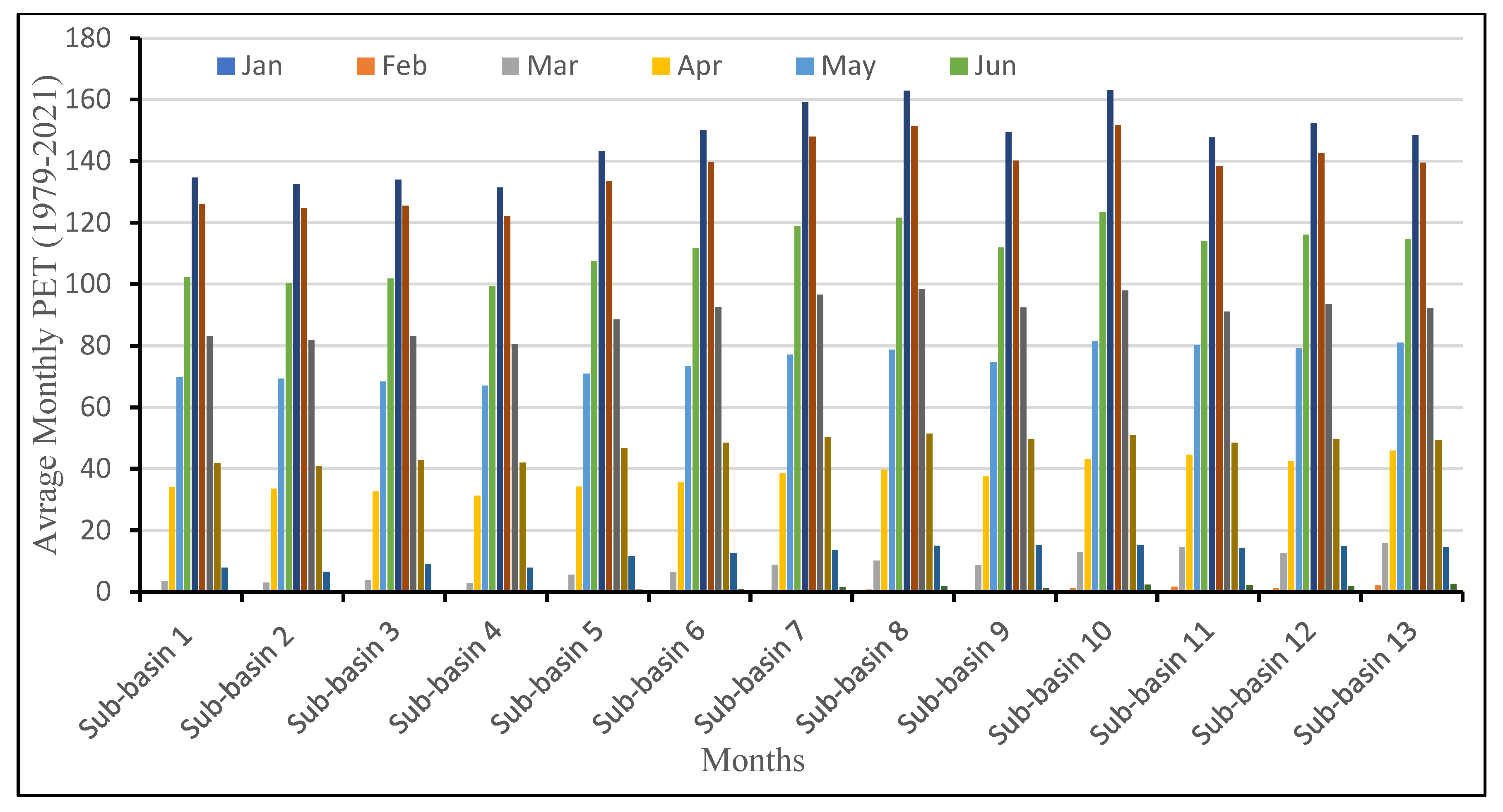
4.1. PET Calculated with the Thornthwaite Equation

R-studio was used to calculate PET with the Thornthwaite equation. The input variables were the temperature and latitude of the Murat Basin, located between 39°N and 43°N in the universal transverse mercator (UTM) system. The process was conducted for all 13 sub-basins, with detailed results provided as supplementary data in the form of Excel sheets (refer to the files labeled as “ PET Results of Thornthwaite Equation”). From the results, a distinct seasonal pattern emerges. During the colder months (January and February), the average temperatures (Tavg) are significantly low, leading to zero or very low PET values across all sub-basins. For instance, in January 1979, the Tavg in Sub-basin 4 was −4.69°C, resulting in a PET of 0.00 mm. Similarly, in February of the same year, Sub-basin 4 maintained a Tavg of −1.57°C with a corresponding PET of 0.00 mm.

As temperatures rise in the spring and summer months (April to August), PET values increase substantially. For example, in May 1979, Sub-basin 4 recorded a Tavg of 11.60°C, resulting in a PET of 66.88 mm, which is a stark contrast to the values observed in January. This trend was further amplified in July 2016, when Sub-basin 4 recorded a Tavg of 21.26°C with a PET of 133.07 mm, indicating the strong influence of temperature on PET during warmer months. The analysis of the relationship between average temperature (Tavg) and potential evapotranspiration (PET) across all sub-basins demonstrates a strong positive correlation, aligning with the principles of the Thornthwaite equation. PET values are negligible or zero when Tavg falls below 0°C, predominantly during the winter months, indicating minimal evaporation potential under cold conditions. As temperatures rise above 0°C in spring, PET begins to increase, with a more pronounced escalation during summer, when Tavg reaches its annual peak.

Across all sub-basins, PET exhibits a consistent upward trend with increasing Tavg, peaking during the summer months (e.g., July and August). However, inter-sub-basin variations point to the influence of local climatic and topographical factors: higher-elevation sub-basins show delayed PET responses due to cooler temperatures, whereas lower-elevation or warmer regions display elevated PET peaks. These findings underscore the high sensitivity of PET to temperature fluctuations and reveal the significant influence of seasonal trends on evapotranspiration-driven water loss. This emphasizes the pivotal role of temperature in regulating evapotranspiration rates and highlights the potential implications of climate variability for regional water resource management.

Figure (4) shows the average monthly PET across 13 sub-basins, derived using the Thornthwaite equation and long-term temperature data spanning 1979 to 2021. The analysis reveals distinct seasonal trends, with PET values peaking during the summer months (June, July, and August) and reaching their lowest in the winter months (December, January, and February) due to average temperature variation. Notably, July records the highest PET values across all sub-basins, exceeding 120 mm, while January exhibits the lowest PET values, falling below 20 mm. Although the general seasonal PET pattern is parallel and consistent, variations in PET values among the sub-basins are noticeable and apparent, the result of influenced by variances in terrain, altitude, and localized climatic circumstances. For example, Sub-basin 5 exhibits slightly reduced PET values during the summer compared to other sub-basins, signifying that higher altitude or cooler local temperatures may mitigate PET in this area. Conversely, Sub-basin 9 demonstrates higher values of PET in both summer and transitional months (May and September), possibly indicating comparatively warmer conditions or lower humidity levels that enhance evaporation rates. Transitional months, such as April and October, also show noticeable variability. Sub-basin 13, for instance, experiences a significant increase in PET in April relative to other sub-basins, representing an earlier beginning of warmer conditions in the region. Likewise, Sub-basin 3 reveals an obvious decline in PET during October, which may mirror former cooling trends or exact microclimatic factors reducing PET during autumn. These findings underscore the heterogeneity of PET dynamics within the area, caused by localized factors such as altitude gradients, microclimatic conditions, and vegetation cover effects. Such sub-basin-specific variations are crucial for effective agricultural planning and water resource management, as highlight extents that might face severe water stress or demand through exact times of the year. For example, sub-basins with constantly high PET values, such as Sub-basin 9, may involve more concentrated irrigation strategies during peak months, whereas zones with lower PET values, such as Sub-basin 5, might certainly experience reduced water stresses. The sub-basin-level detail provided by this PET analysis offers a valuable understanding of sustainable water resource management. It emphasizes the essential to account for spatial variability in climate-driven factors when scheming irrigation systems, approximating water accessibility, and preparing climate adaptation actions within the region.

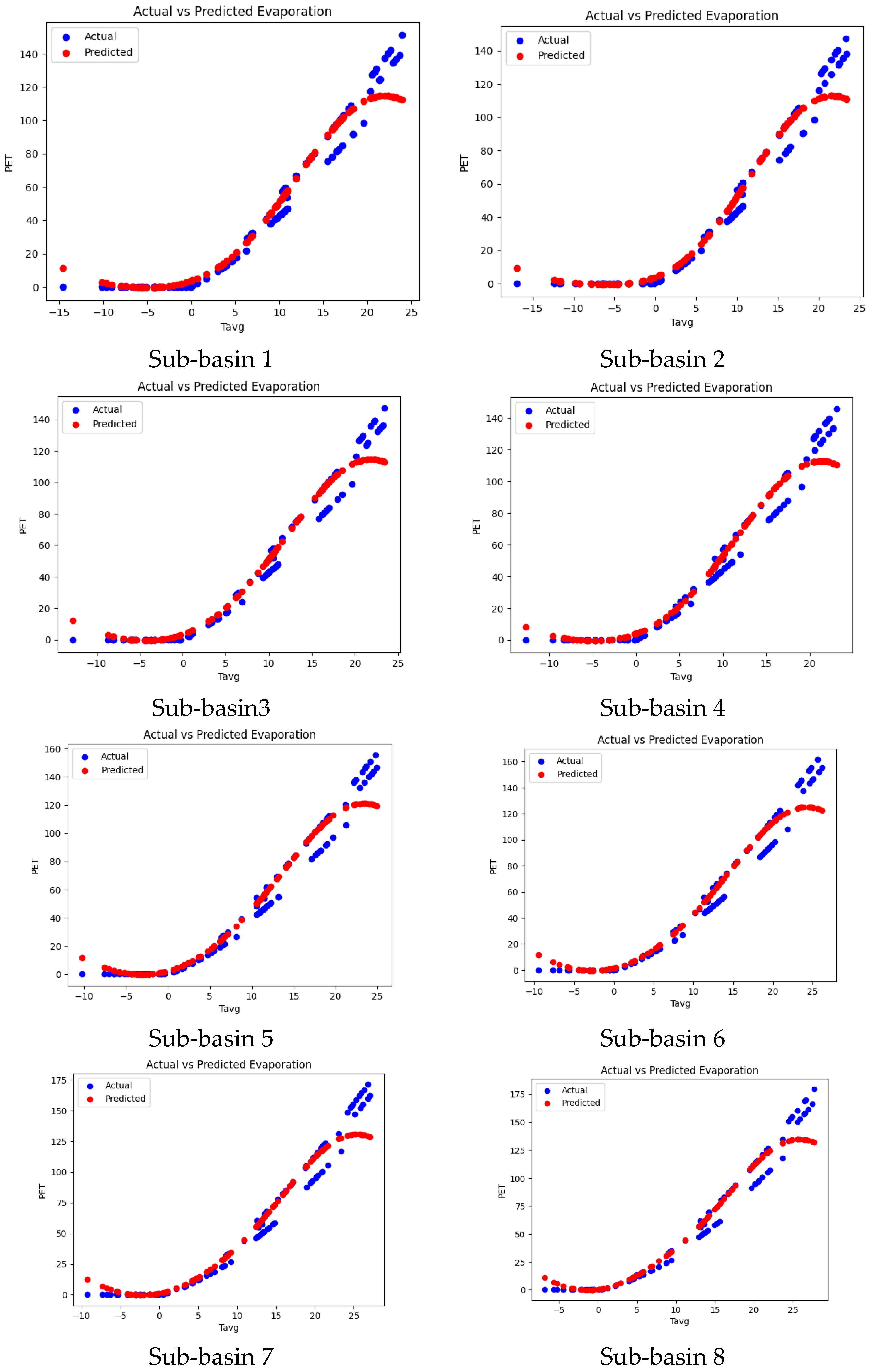
4.2. PET Prediction via CNN

The findings reveal a strong correlation between observed and predicted PET values across most sub-basins, underscoring the CNN model’s effectiveness in estimating PET. In the graphical outputs, red lines represent predicted values, while blue points depict observed measurements; ideally, these points align closely with the red line, indicating high predictive accuracy. Sub-basins 1, 5, 8, and 10 display a clear linear relationship, with predicted values closely mirroring observed data. In contrast, Sub-basins 3 and 12 contain some outliers, suggesting that minor adjustments to model calibration may enhance accuracy. Notably, Sub-basins 6 and 7 show more pronounced deviations, indicating possible inconsistencies that merit further investigation into factors affecting evaporation in these regions. Overall, the model performs robustly across the majority of sub-basins, suggesting a strong capacity to generalize across diverse geographic and climatic conditions (Figure 5). Although the CNN model demonstrates considerable promise for predicting potential evaporation, addressing the identified outliers will further improve its predictive accuracy. Future model enhancements, such as hyperparameter tuning and integrating additional data sources, could also improve performance in more variable regions.

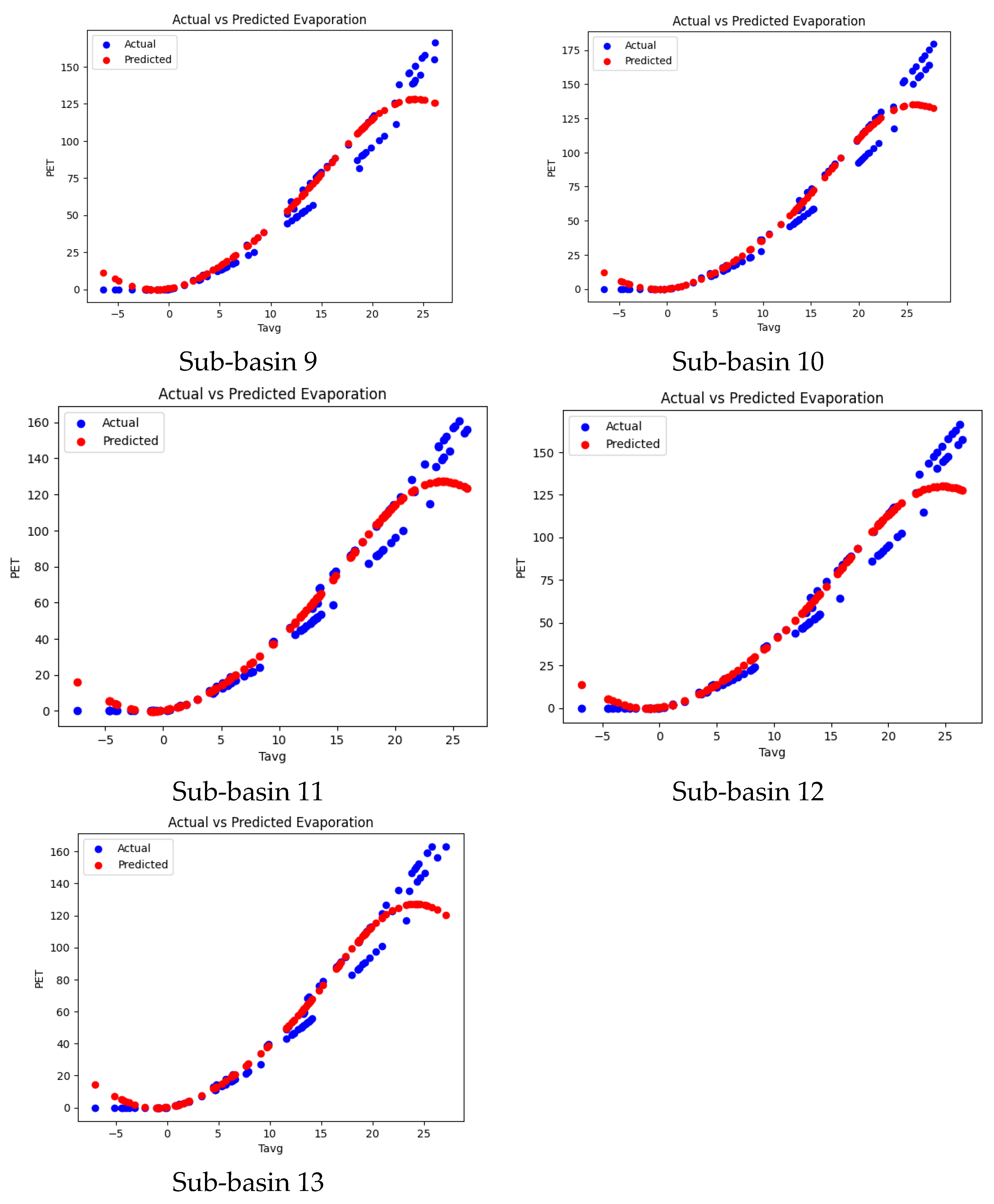
4.3. PET Prediction via SVM

The SVM model demonstrates robust and reliable performance across all sub-basins, with metrics indicating high R² and low MSE AND RMSE, underscoring its suitability for predictive tasks in diverse sub-regional contexts, which is parallel to previous studies [38,39].

The results provide a comparative analysis of actual and predicted PET across 13 sub-basins, modeled using an SVM. Each sub-basin is represented by a graph that plots PET against temperature (denoted as “Temp,” likely in degrees Celsius). Blue dots indicate the observed recorded PET values, while a red dashed line illustrates the PET values predicted by the SVM model. In each plot, predicted values (blue dots) are displayed alongside observed values (red dots), and the alignment of these points demonstrates a strong correlation between predictions and observations. This close alignment reflects the model’s high accuracy in estimating PET. Across all sub-basins, a positive correlation between temperature and PET is evident; as temperature rises, so does PET (Figure 6). This trend aligns with expectations, as higher temperatures generally increase evaporation and plant transpiration.

The SVM model appears to perform reasonably well in most sub-basins, as the red prediction line generally follows the trend of the actual PET data. However, predictive accuracy varies among sub-basins. In some cases, the predicted line closely matches the real values, indicating a strong fit, while in others, noticeable deviations particularly at higher temperatures propose slight overestimations or underestimations by the model. Certain sub-basins, such as 1, 2, and 3, exhibit a more linear relationship between temperature and PET, while others, including sub-basins 7 and 10, display a more curvilinear pattern. This variation may reflect differing local environmental factors, such as vegetation cover, soil type, and water availability, which can affect PET behavior. Notably, sub-basin 12 demonstrates lower PET values across the temperature range in comparison to other sub-basins, suggesting unique characteristics influencing PET in this area.

The graphic advocates that projected and observed PET by SVM model are effective for PET estimation across diverse hydrological settings, each with unique environmental conditions, highlighting its potential applications in water resource management and hydrological modeling [38,40].

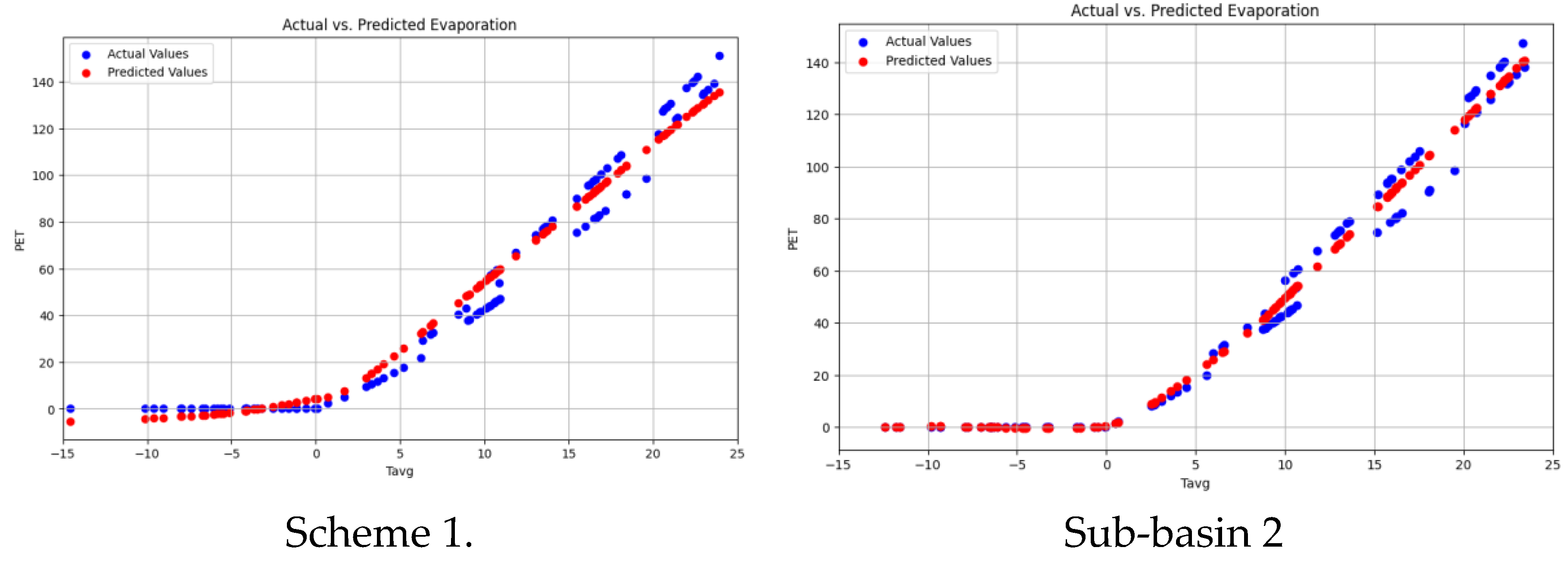
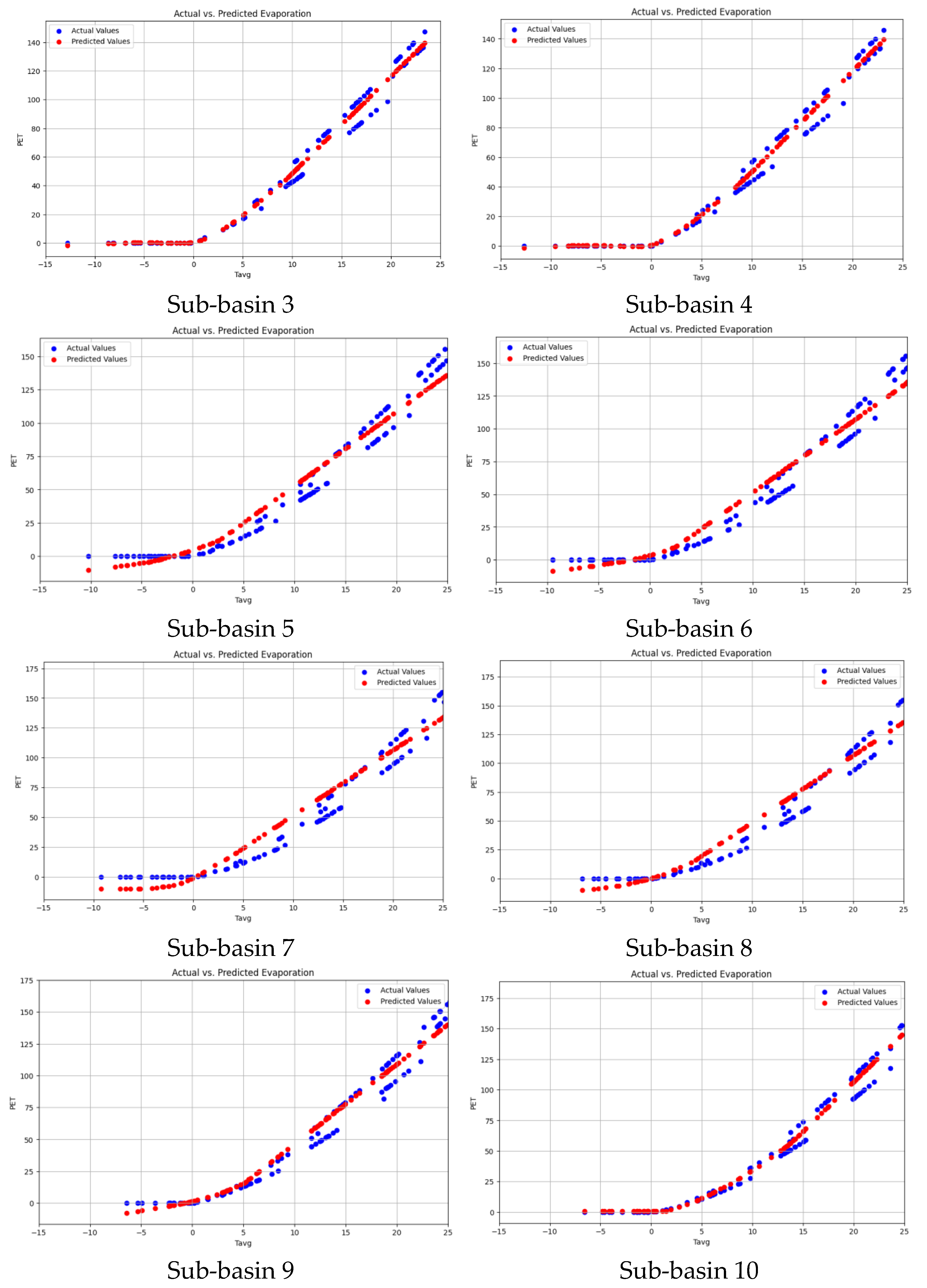
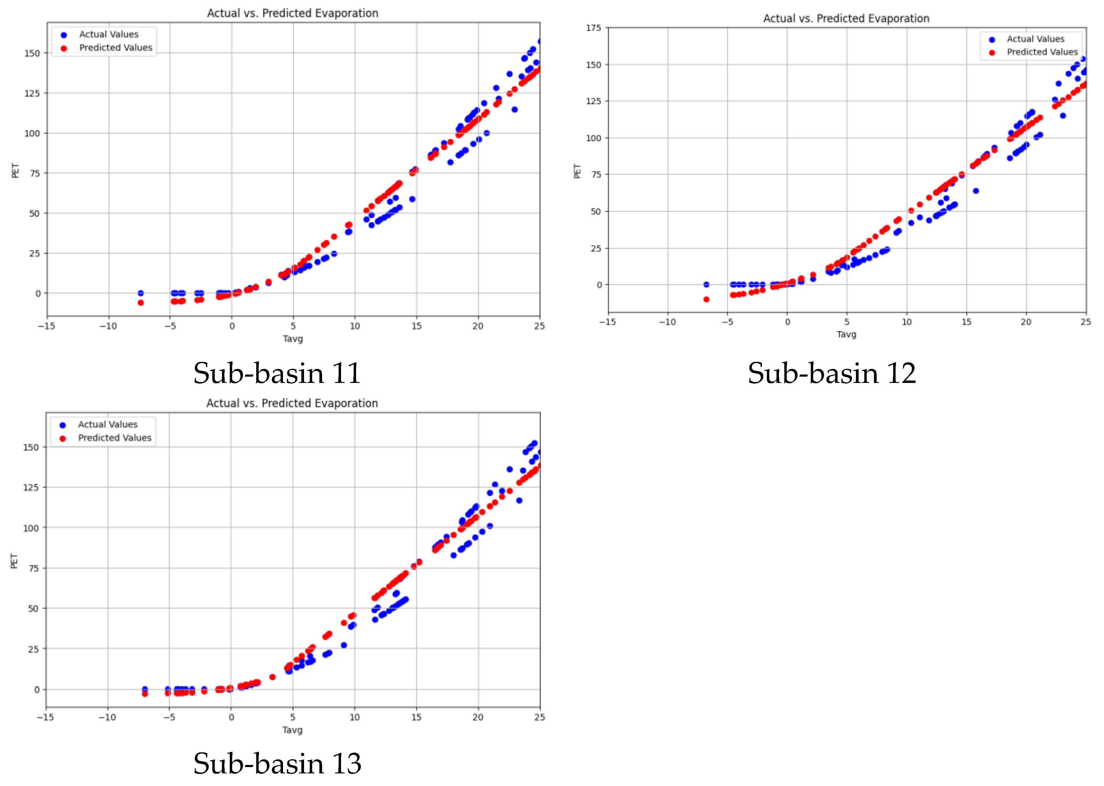
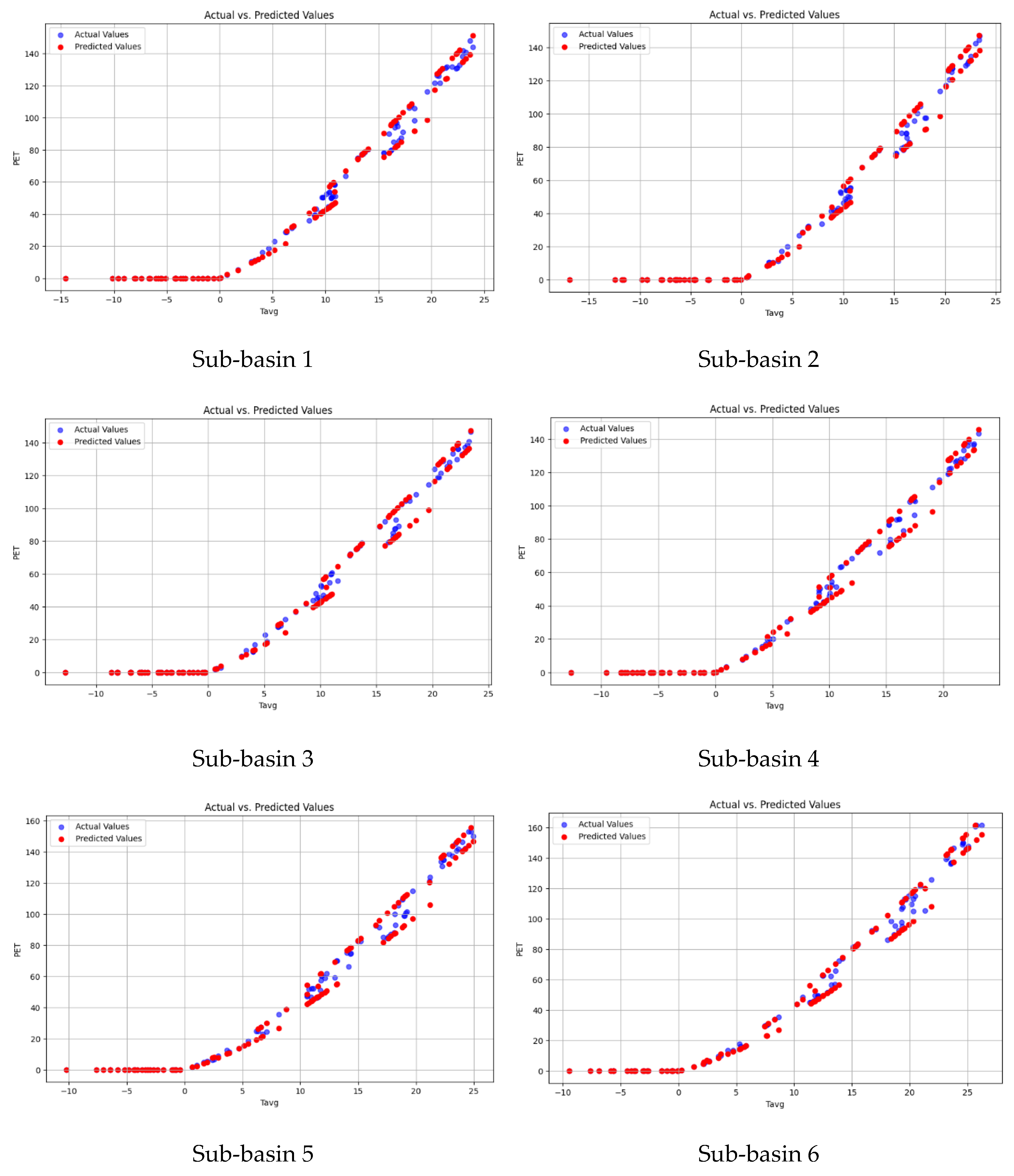
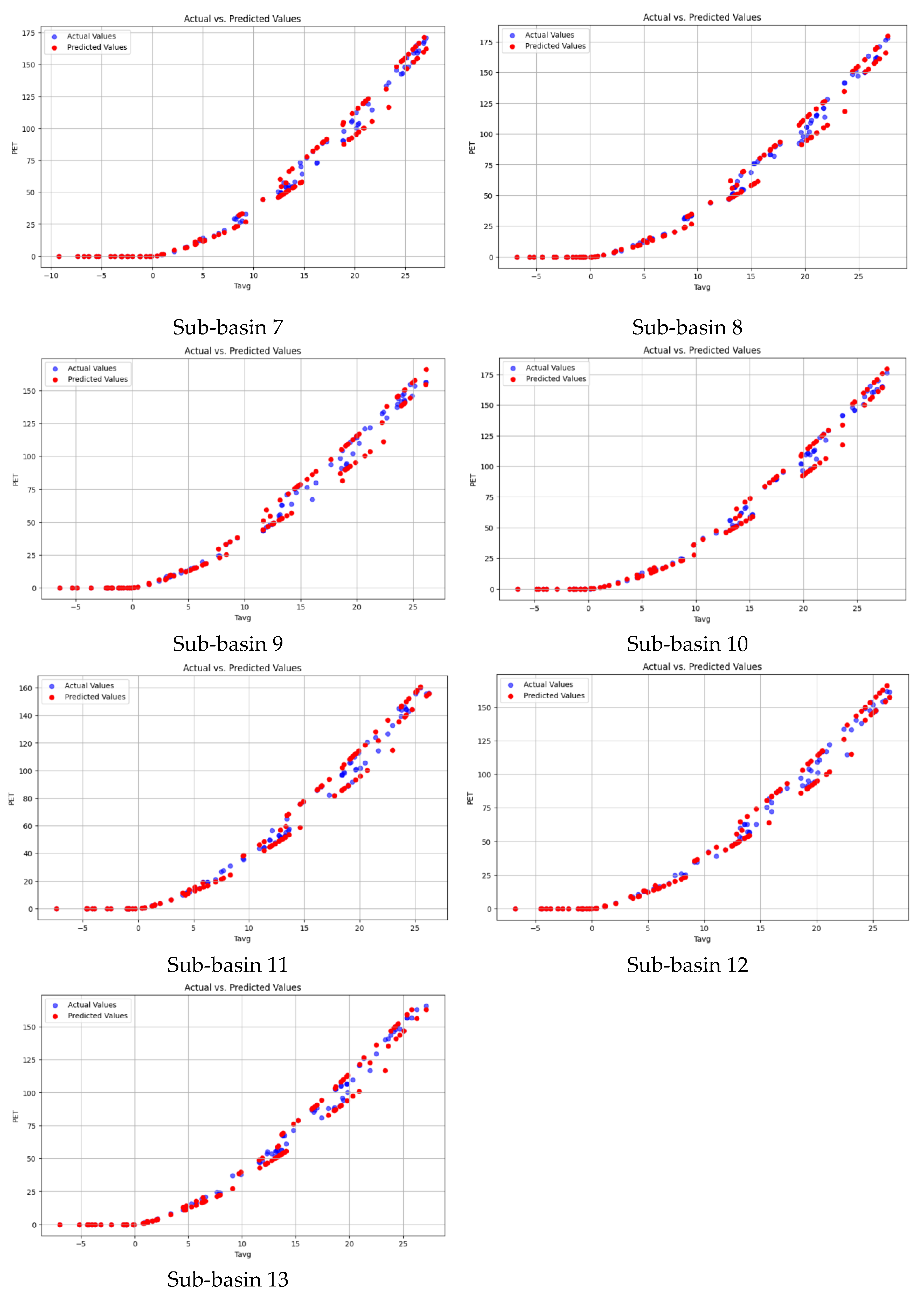
4.4. PET Prediction via RF

After obtaining predictions from each decision tree, the final results for the regression problem were determined by averaging the outputs of all trees. For the classification problem, the final result was derived from a majority vote among all trees. The RF model can overcome the high-dimensional data and strong nonlinear problems, reducing the overfitting by averaging the results [39]. The results demonstrate the RF model’s superiority in this context, making it a highly suitable choice for accurate and dependable PET predictions across diverse sub-basins.

Figure (7) demonstrates an evaluation of an RF model’s predictions of PET across 13 sub-basins by comparing observed measured data and predicted values. Each of the 13 plates corresponds to a specific sub-basin. Each subplot represents the model’s performance, with points aligned along the diagonal 1:1 line indicating accurate predictions. The results reveal strong predictive performance across most sub-basins, with minimal deviations, particularly in low and mid-range PET values. However, slight underestimations are observed at higher PET values in sub-basins such as 7, 8, and 10. Sub-basins 3, 5, and 12 exhibit tightly clustered points along the diagonal, demonstrating robust accuracy, while sub-basins 2 and 6 show minor scatter, suggesting some variability in predictions. These observations highlight the model’s general effectiveness while indicating areas for potential refinement.

The results indicate the model performs well across most sub-basins, as seen in the scatter plots, which reveal a positive correlation between observed and predicted values. In many sub-basins, this relationship is particularly strong, highlighting the model’s capability to capture overall patterns in PET. In some scatter plots, deviations from the ideal line indicate chance inaccuracies, which are commonly assumed the complexity of real-world processes. However, the visualization reveals that the model offers a valuable estimate of PET, offering insights that could be applied in water resource management and ecological research. To further quantify and analyze model performance, metrics such as R², RMSE, and MAE should be incorporated. Additionally, conducting a feature importance analysis and addressing the higher-range deviations could enhance the model’s reliability and provide insights for improved performance in specific sub-basins.

4.5. Performance of the Models

Table (3) provides a comprehensive assessment of the performance of three algorithms CNN, SVM, and RF in expecting PET results across 13 sub-basins based on average temperature. There are three statistical metrics have been used for assessing the result of proposed models including R², MSE, and RMSE. Below is a detailed analysis of each metric.

Among the models, RF consistently reveals superior performance, attaining the highest R² values (1.000) across all sub-basins. These findings indicate that RF effectively captures the relationship between the predictor (average temperature) and target variables (PET) with perfect accuracy. While MSE and RMSE values varied slightly among the sub-basins, they offer additional insights into the model’s predictive precision. Moreover, RF accomplishes the lowest MSE and RMSE values in all sub-basins, with mostly strong performance in sub-basin 2 (MSE = 0.326, RMSE = 0.571) and sub-basin 13 (MSE = 0.385, RMSE = 0.621). Conversely, sub-basin 8 exhibited the highest MSE (0.640) and RMSE (0.649), reflecting relatively larger prediction errors. These results advocate greater prediction challenges in these areas, possibly due to increased data inconsistency or more complex underlying patterns. Despite these differences, the RMSE values across all sub-basins remained consistently low, further validating the model’s effectiveness in minimizing errors. These findings underscore RF’s capacity to moderate prediction errors and establish it as the most vigorous model for this dataset. The RF model’s consistently high accuracy, combined with low MSE and RMSE values, highlights its robustness and reliability in predicting PET across diverse sub-regions. This exceptional performance can be attributed to the model’s ability to manage complex datasets effectively and mitigate overfitting through its ensemble learning approach. By combining multiple decision trees, the RF model enhances predictive accuracy and generalization, making it an ideal tool for precise PET estimation across varying climatic and topographic conditions {15}.

The CNN model also exhibits strong predictive capabilities, with R² values spanning from 0.962 to 0.987. Its best performance is observed in sub-basin 5, where it attains an MSE of 0.277 and an RMSE of 0.526, reflecting high accuracy. Notable results are also observed in sub-basin 3 (R² = 0.987, MSE = 0.309, RMSE = 0.556) and sub-basin 9 (R² = 0.987, MSE = 0.405, RMSE = 0.637). However, CNN consistently records slightly higher errors compared to RF across most sub-basins, suggesting it is less effective overall. Despite this, CNN remains a reliable model, though its computational intensity relative to RF may pose practical challenges depending on the application.

In contrast, the SVM algorithm shows mixed performance, with notable weaknesses in certain sub-basins. While its R² values are relatively stable and dependable, ranging from 0.945 to 0.956, it exhibits higher error rates in several regions. For example, in sub-basins 7 and 9, SVM struggles with high MSE values of 0.981 and 1.013 and corresponding RMSE values of 0.990 and 1.014, indicating reduced predictive reliability in areas with greater data complexity or climate variability. However, SVM performs relatively well in sub-basins 5 and 3, attaining lower error rates (MSE = 0.267 and 0.287, respectively). Despite these strengths, SVM’s overall performance is weaker than both RF and CNN, limiting its suitability for this application.

In general, Random Forest emerges as the most effective, and outperforms other models and dependable algorithms, achieving exceptional accuracy and minimal prediction errors across all sub-basins. CNN offers a viable alternative with consistent and strong performance, particularly in sub-basins 5 and 3, though it slightly lags behind RF. On the other hand, SVM demonstrates the weakest overall performance, with notable challenges in sub-basins 7 and 9, suggesting it is less appropriate for this dataset. These results emphasize the robustness of RF in handling data variability, making it the preferred choice for this predictive task.

5. Conclusion

This study delivers an inclusive assessment of machine learning and deep learning models including Support Vector Machine (SVM), Convolutional Neural Network (CNN), and Random Forest (RF) for predicting PET in the Murat River Basin. Using forty years of monthly temperature data and the temperature-based Thornthwaite equation, this research effectively tackles the challenge of PET prediction in regions with limited data accessibility by integrating advanced computational methods.

The findings indicate that the RF model outperformed other models, achieving a perfect R² value of 1.000 across all sub-basins, along with the lowest MSE and RMSE values. This excellent performance is attributed to the RF model’s ability to manage complex datasets, reduce overfitting, and accurately capture nonlinear relationships. CNN also established strong predictive accuracy, leveraging its deep learning architecture to recognize complicated patterns within the dataset. While SVM provided reliable predictions, its performance was more sensitive to data quality and hyperparameter differences, making it most operative in sub-basins with simpler or more linear relationships. The spatial and temporal investigation of PET trends exposed notable seasonal fluctuations, with PET values peaking in the summer months and showing a strong positive correlation with increasing temperatures. These results highlight the essential role of temperature in driving evapotranspiration processes, particularly in semi-arid regions where effective water management is critical for ensuring agricultural sustainability. Integrating GIS spatial modeling additionally improved PET prediction accuracy by accounting for variations in topography and climate across the basin. This study underscores the potential of artificial intelligence-driven models to enhance PET estimations, offering valuable contributions to hydrological modeling, water resource management, and agricultural planning in the face of climate change. The RF model, acknowledged as the most robust and accurate, offers a transferable methodology that can be adapted to other regions with similar data limitations. Future research would aim to integrate extra climatic parameters, improve model standardization techniques, and explore collaborative modeling methods to further improve prediction accuracy and generalizability.

By advancing PET prediction methodologies, this research significantly contributes to hydrological science, addressing the pressing essential for data-efficient and accurate modeling approaches to meet the challenges posed by climate variability and growing water demand.

References

1. Wood, E. F. , Su, H. , McCabe, M., & Su, B. (2003). Estimating evaporation from satellite remote sensing. Paper presented at the IGARSS 2003. 2003 IEEE International Geoscience and Remote Sensing Symposium. Proceedings (IEEE Cat. No. 03CH37477). [Google Scholar]
2. Jing, W. , Yaseen, Z. M., Shahid, S., Saggi, M. K., Tao, H., Kisi, O.,... Chau, K.-W. Implementation of evolutionary computing models for reference evapotranspiration modeling: short review, assessment, and possible future research directions. Engineering applications of computational fluid mechanics 2019, 13, 811–823. [Google Scholar] [CrossRef]
3. Raman, J. , Kim, J.-S., Choi, K. R., Eun, H., Yang, D., Ko, Y.-J., & Kim, S.-J. Application of lactic acid bacteria (LAB) in sustainable agriculture: Advantages and limitations. International Journal of Molecular Sciences 2022, 23, 7784. [Google Scholar] [PubMed]
4. Pelosi, A. , Villani, P., Falanga Bolognesi, S., Chirico, G. B., & D’Urso, G. Predicting crop evapotranspiration by integrating ground and remote sensors with air temperature forecasts. Sensors 2020, 20, 1740. [Google Scholar]
5. Penman, H. L. Natural evaporation from open water, bare soil, and grass. Proceedings of the Royal Society of London. Series A. Mathematical and Physical Sciences 1948, 193, 120–145. [Google Scholar]
6. Shuttleworth, W. (1993). Evaporation Handbook of Hydrology ed DR Maidment. In: New York: McGraw-Hill) pp.
7. Allen, R. G. , Clemmens, A. J., Burt, C. M., Solomon, K., & O’Halloran, T. Prediction accuracy for projectwide evapotranspiration using crop coefficients and reference evapotranspiration. Journal of irrigation and drainage engineering 2005, 131, 24–36. [Google Scholar]
8. Aschonitis, V. , Touloumidis, D., ten Veldhuis, M.-C., & Coenders-Gerrits, M. Correcting Thornthwaite potential evapotranspiration using a global grid of local coefficients to support temperature-based estimations of reference evapotranspiration and aridity indices. Earth System Science Data 2022, 14, 163–177. [Google Scholar]
9. Brutsaert, W. Global land surface evaporation trend during the past half-century: Corroboration by Clausius-Clapeyron scaling. Advances in Water Resources 2017, 106, 3–5. [Google Scholar] [CrossRef]
10. Bouchet, R. (1963). Evapotranspiration reelle, evapotranspiration potentielle, et production agricole. Paper presented at the Annales agronomiques.
11. Thornthwaite, C. W. An approach toward a rational classification of climate. Geographical Review 1948, 38, 55–94. [Google Scholar] [CrossRef]
12. Ahmadi, F. , Mehdizadeh, S., Mohammadi, B., Pham, Q. B., Doan, T. N. C., & Vo, N. D. Application of an artificial intelligence technique enhanced with intelligent water drops for monthly reference evapotranspiration estimation. Agricultural Water Management 2021, 244, 106622. [Google Scholar]
13. Fahimi, F. , Yaseen, Z. M., & El-Shafie, A. Application of soft computing based hybrid models in hydrological variables modeling: a comprehensive review. Theoretical and applied climatology 2017, 128, 875–903. [Google Scholar]
14. Mehr, A. D. , Nourani, V., Kahya, E., Hrnjica, B., Sattar, A. M., & Yaseen, Z. M. Genetic programming in water resources engineering: A state-of-the-art review. Journal of Hydrology 2018, 566, 643–667. [Google Scholar]
15. Shahbazi, A. N. , Zahraie, B., & Nasseri, M. (2012). Seasonal meteorological drought prediction using support vector machine.
16. Chen, Z. , Sun, S., Wang, Y., Wang, Q., & Zhang, X. Temporal convolution-network-based models for modeling maize evapotranspiration under mulched drip irrigation. Computers and electronics in agriculture 2020, 169, 105206. [Google Scholar]
17. Hassan, M. A. , Khalil, A., Kaseb, S., & Kassem, M. Exploring the potential of tree-based ensemble methods in solar radiation modeling. Applied Energy 2017, 203, 897–916. [Google Scholar]
18. Papadopoulos, S. , Azar, E., Woon, W.-L., & Kontokosta, C. E. Evaluation of tree-based ensemble learning algorithms for building energy performance estimation. Journal of Building Performance Simulation 2018, 11, 322–332. [Google Scholar]
19. Granata, F. , & Di Nunno, F. Forecasting evapotranspiration in different climates using ensembles of recurrent neural networks. Agricultural Water Management 2021, 255, 107040. [Google Scholar]
20. Deng, L. , & Yu, D. Deep learning: methods and applications. Foundations and trends® in signal processing 2014, 7, 197–387. [Google Scholar]
21. Fattah, W. H. , & IMi, Y. Hydrological analysis of Murat river basin. International Journal of Applied 2015, 5, 47–55. [Google Scholar]
22. Terakawa, A. (2003). Hydrological data management: Present state and trends: Secretariat of the World Meteorological Organization.
23. Naoum, S. , & Tsanis, I. Ranking spatial interpolation techniques using a GIS-based DSS. Global Nest 2004, 6, 1–20. [Google Scholar]
24. Chai, H. , Cheng, W., Zhou, C., Chen, X., Ma, X., & Zhao, S. Analysis and comparison of spatial interpolation methods for temperature data in Xinjiang Uygur Autonomous Region, China. Natural Science 2011, 3, 999. [Google Scholar]
25. Anggraini, N. , & Slamet, B. (2021). Thornthwaite Models for Estimating Potential Evapotranspiration in Medan City. Paper presented at the IOP Conference Series: Earth and Environmental Science. [Google Scholar]
26. Azman, R. , Noor, N., Abdullah, S., & Ideris, M. Analysis of Drought Index in Sub-Urban Area Using Standard Precipitation Evapotranspiration Index (SPEI). International Journal of Integrated Engineering 2022, 14, 157–163. [Google Scholar]
27. Kim, S.-J. , Bae, S.-J., & Jang, M.-W. Linear regression machine learning algorithms for estimating reference evapotranspiration using limited climate data. Sustainability 2022, 14, 11674. [Google Scholar]
28. Pramanik, M. , Chowdhury, K., Rana, M. J., Bisht, P., Pal, R., Szabo, S., Pal, I., Behera, B., Liang, Q., Padmadas, S. S., & Udmale, P. Climatic influence on the magnitude of COVID-19 outbreak: a stochastic model-based global analysis. International Journal of Environmental Health Research 2022, 32. [Google Scholar] [CrossRef]
29. Wang, Q. , Ma, Y., Zhao, K., & Tian, Y. A Comprehensive Survey of Loss Functions in Machine Learning. Annals of Data Science 2022, 9. [Google Scholar] [CrossRef]
30. Tian, Y. , Su, D., Lauria, S., & Liu, X. (2022). Recent advances in loss functions in deep learning for computer vision. In Neurocomputing (Vol. 497). [CrossRef]
31. Lee, J. K. , Rouault, M., & Wyart, V. Adaptive tuning of human learning and choice variability to unexpected uncertainty. Science Advances 2023, 9. [Google Scholar] [CrossRef]
32. Liu, S. , & Zhou, D. J. Using cross-validation methods to select time series models: Promises and pitfalls. British Journal of Mathematical and Statistical Psychology 2024, 77. [Google Scholar] [CrossRef]
33. Siva, G. Matrix variate receiver operating characteristic curve for binary classification. Statistics 2024, 58. [Google Scholar] [CrossRef]
34. Breiman, L. Random forests. Machine learning 2001, 45, 5–32. [Google Scholar] [CrossRef]
35. Lazar, J. , Feng, J. H., & Hochheiser, H. (2017). Research methods in human-computer interaction: Morgan Kaufmann.
36. Brito, L. C. , Pecanha, T. , Fecchio, R. Y., Rezende, R. A., Sousa, P., Silva-Junior, D.,... Halliwill, J. R. Morning versus evening aerobic training effects on blood pressure in treated hypertension. Medicine and science in sports and exercise 2019, 51, 653–662. [Google Scholar] [CrossRef] [PubMed]
37. Feng, F. , Tuomi, M., Jones, H. R., Barnes, J., Anglada-Escude, G., Vogt, S. S., & Butler, R. P. Color difference makes a difference: four planet candidates around τ ceti. The Astronomical Journal 2017, 154, 135. [Google Scholar]
38. Yaseen, Z. M. , Al-Juboori, A. M., Beyaztas, U., Al-Ansari, N., Chau, K.-W., Qi, C.,... Shahid, S. Prediction of evaporation in arid and semi-arid regions: A comparative study using different machine learning models. Engineering applications of computational fluid mechanics 2020, 14, 70–89. [Google Scholar] [CrossRef]
39. Lee, Y. C. , Christensen, J. J., Parnell, L. D., Smith, C. E., Shao, J., McKeown, N. M., Ordovás, J. M., & Lai, C. Q. Using Machine Learning to Predict Obesity Based on Genome-Wide and Epigenome-Wide Gene–Gene and Gene–Diet Interactions. Frontiers in Genetics 2022, 12. [Google Scholar] [CrossRef]
40. Wald, N. J. , & Bestwick, J. P. Is the area under an ROC curve a valid measure of the performance of a screening or diagnostic test? Journal of Medical Screening 2014, 21. [Google Scholar] [CrossRef]
Figure 1. Location of Murat River Basin between Turkey Basins.
Preprints 141322 g001
Figure 2. Sub-basins of the Murat River Basin extracted by Arc-Map.
Preprints 141322 g002
Figure 3. Thiessen polygon method applied to meteorological stations in the Murat Basin.
Preprints 141322 g003
Figure 4. Average monthly PET calculated with Thornthwaite equation (1979-2021).
Preprints 141322 g004
Figure 5. Actual and predicted PET calculated via CNN.
Preprints 141322 g005aPreprints 141322 g005bPreprints 141322 g005c
Figure 6. Predicted and actual PET via SVM.
Preprints 141322 g006aPreprints 141322 g006b
Figure 7. Actual and predicted PET via RF.
Preprints 141322 g007aPreprints 141322 g007b