1. Introduction
Climate change remains one of the most formidable global challenges of the twenty-first century, exerting profound impacts on hydrological systems, ecosystems, and human livelihoods [
1]. Increasing evidence shows that intensifying climatic change has led to more frequent and severe floods, droughts, and prolonged dry spells, disrupting agricultural productivity and threatening water and food security worldwide [
1,
2,
3]. Globally, such events have displaced an estimated 22 million people annually since 2008, emphasizing the growing humanitarian extent of hydrological extremes [
4]. Global assessments further indicate that under continued warming, some regions will experience enhanced surface runoff and flood risk, while others will face pronounced drying trends [
3]. The Intergovernmental Panel on Climate Change (IPCC) Sixth Assessment Report projects a potential rise in global mean temperature of up to 1.5 °C above pre-industrial levels by the early 2030s, accompanied by intensified precipitation extremes, prolonged droughts, and accelerated sea-level rise between 0.3 m and 1.1 m by 2100 [
1]. These shifts are continually driving countries around the world to adopt adaptation measures to enhance resilience and mitigate escalating hydrological risks at both local and basin scales [
5,
6,
7].
In response to these evolving climatic pressures, structural interventions have become central to national and regional adaptation strategies across many parts of the world. Governments and water management authorities are increasingly constructing dams, retention basins, and concrete-lined drainage systems to control floods and secure water supply for domestic and agricultural use [
8]. While such measures play a vital role in safeguarding infrastructure and livelihoods, they also introduce significant alterations to natural hydrological regimes [
5]. These modifications change infiltration capacity, channel roughness, and storage dynamics, thereby influencing the magnitude, timing, and duration of peak flows [
9]. Previous studies have reported that channel concretization accelerates runoff concentration and reduces groundwater recharge, whereas dam construction alters downstream hydrographs [
7,
10,
11]. Understanding the impact of these measures on runoff in a watershed is a critical aspect of water resource management and hydrological studies [
12,
13,
14]. For instance, Huang et al. [
15] demonstrated that increased structural modification by increasing imperviousness hindered the infiltration of runoff and caused it to flow directly into rivers, ultimately increasing both surface and channel runoff. Their findings gave implications for prioritizing measures in flood prevention and preparedness, such as the consideration of building arrangement, green infrastructure, and the Low Impact Development (LID) techniques.
Assessing the effects of interventions has become an essential component of modern watershed management and climate adaptation planning [
16,
17]. Researchers have employed approaches to evaluate the hydrological impacts of anthropogenic interventions in watershed systems. Studies such as those by Rose and Peters [
18], Miller et al. [
19] and Ress et al. [
6] applied paired-catchment analyses to compare runoff responses between drained and undrained basins, demonstrating that artificial drainage increases surface runoff and shortens flow concentration times. More recent studies have advanced to process-based and data-driven frameworks that couple hydrological and statistical methods [
20,
21,
22]. For instance, Song et al. [
20] combined the SIMHYD rainfall–runoff model, the Budyko framework, and double-mass curve (DMC) analysis to quantify the hydrological alterations induced by mining in the headwaters of Chinese catchments, reporting consistent evidence of substantial flow modification across all methods. Similarly, Zhang et al. [
21] used both DMC and hydrological modelling to assess irrigation and mining impacts in the Qingshui River Basin, revealing significant declines in streamflow. While the DMC technique provides a simple means of detecting regime shifts, it cannot reproduce natural flow processes under non-stationary or structurally modified conditions, or during specific rainfall events [
23]. In contrast, physically based hydrological models have demonstrated greater capability to reproduce natural streamflow regimes because they incorporate watershed characteristics such as soils, slopes, land use, and climatic variables [
20,
24]. When integrated with hydraulic analysis, these models can effectively capture spatially distributed hydrological responses to observed rainfall events by accounting for both channel and catchment-scale flow dynamics [
25].
HEC-RAS two-dimensional (2D) rain-on-grid modelling has emerged as a powerful approach for simulating coupled hydrologic–hydraulic processes. Its rain-on-grid capability enables direct application of rainfall events onto a two-dimensional computational mesh, allowing dynamic interaction between surface runoff, catchment characteristics, and channel flow [
26]. Despite its growing use in floodplain and urban drainage studies worldwide [
8,
11,
27], few studies have employed this approach to evaluate the effects of structural interventions such as dam storage and concrete-lined drains on high-flow behaviour at a catchment scale. In addition, the simulation structural interventions form a scientific basis for identifying locations where Nature-Based Solutions (NbS) can be implemented and would most effectively enhance flood mitigation and complement existing civil engineering infrastructure [
16,
28,
29].
This study seeks to contribute knowledge by assessing the high-flow characteristics of the Chongwe River Catchment in Zambia using HEC-RAS 6.5, particularly terrain modification tools. Terrain modification provides a low-cost approach for adjusting freely available DEMs to incorporate small-scale engineered features without the need for detailed topographic surveys, such as drone-based mapping [
30]. Within the Chongwe Catchment, two major structural-based interventions have already been implemented, namely: (i) concrete-lining of natural river channels in urban Lusaka for flood management, and (ii) construction of ten dams on the rivers primarily for irrigation and domestic water supply [
31,
32,
33]. Despite their scale and significance, the hydrological impacts of these measures on the observed high-flow characteristics of the Chongwe River during extreme rainfall events remain poorly understood at the catchment scale. Moreover, to the best of our knowledge, no study has undertaken rainfall-event-based modelling of flows within the Chongwe Catchment. Our study, therefore, provides a low-cost novel approach to how engineered river catchment modifications affect hydrological responses, giving transferable approaches for assessing infrastructure-driven flood dynamics in data-scarce river catchments and an opportunity for improvement in future planning.
4. Conclusions and Recommendations
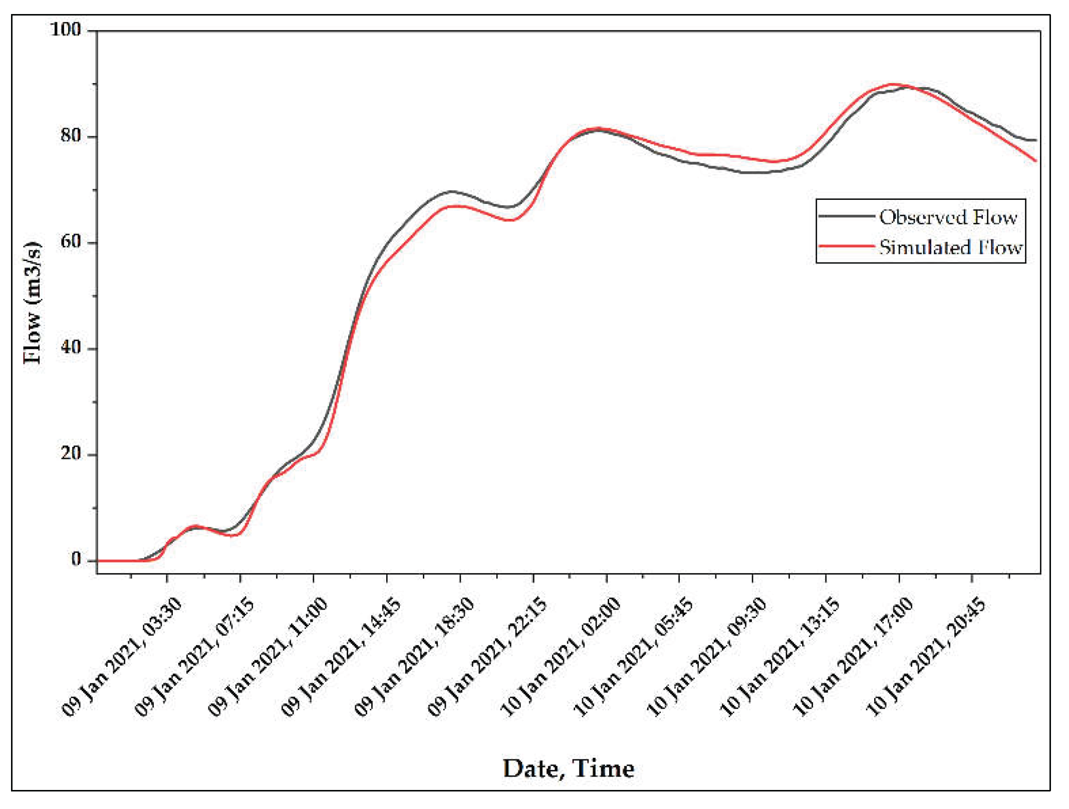
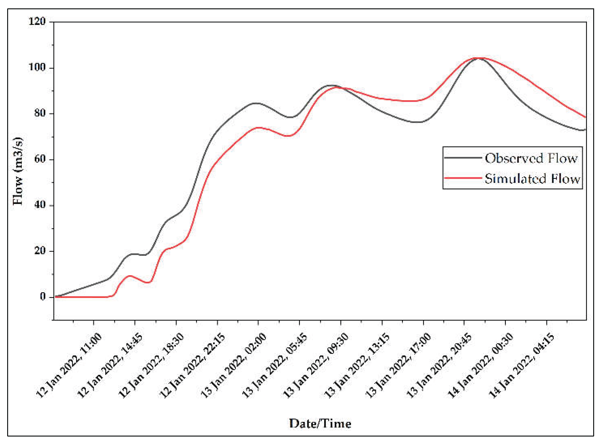
This study used a 2D rain-on-grid HEC-RAS event-based modelling approach to evaluate the influence of concrete-lining of natural channels and dam storage on high-flow behaviour in the Chongwe River Catchment. The model performed well with R2 = 0.99, NSE = 0.75, and PBIAS = −0.68% for calibration, and R2 = 0.95, NSE = 0.75, and PBIAS = −2.49% for validation. This shows that the model is suitable for event-based flood modelling in the Chongwe Catchment and similar catchments. The study demonstrated that the concrete-lining of 21 km of natural drainage channels in Lusaka increased high flows by approximately 4.6% at the main catchment outlet and generated very high flow velocities within the urban drainage system. On the other hand, the 10 existing dams reduced peak flows by about 28% and increased lag times by 24%, while flood depth and flood extent reduced by 10% and 4%, respectively. This demonstrates their important role in reducing the magnitude of flash floods. Future urban planning should incorporate downstream storage infrastructure such as dams, alongside major drainage upgrades to effectively capture stormwater and mitigate the high-flow impacts associated with the concrete-lining of natural channels. Additionally, literature has shown that concrete-lining of natural channels in urban areas can affect the runoff water quality through geochemical interactions between stormwater and concrete surfaces. Therefore, planning efforts should holistically consider both quantity and quality aspects to ensure that downstream water bodies, including dams, maintain acceptable water quality standards for domestic and agricultural use.
The limitations of the study include: (i) the use of event-based simulation rather than continuous long-term modelling, which does not capture seasonal hydrological variability or dam operation dynamics; (ii) simplified river channel representation due to sparse cross-section data and manual interpolation, which may introduce geometric uncertainty in modified channels and dam structures; and (iii) the assumption of uniform rainfall distribution across the catchment, which may overlook spatial rainfall variability during localized storms. Future research could also benefit from continuous modelling over longer periods to quantify the effects of dams under a wider range of hydrometeorological conditions. For sub-catchments such as Kanakantapa, where no significant structural modifications were observed but rain-fed agriculture is predominant [
34], further assessment of land management and soil conditions is needed to guide the selection of suitable interventions across the Chongwe River Catchment.
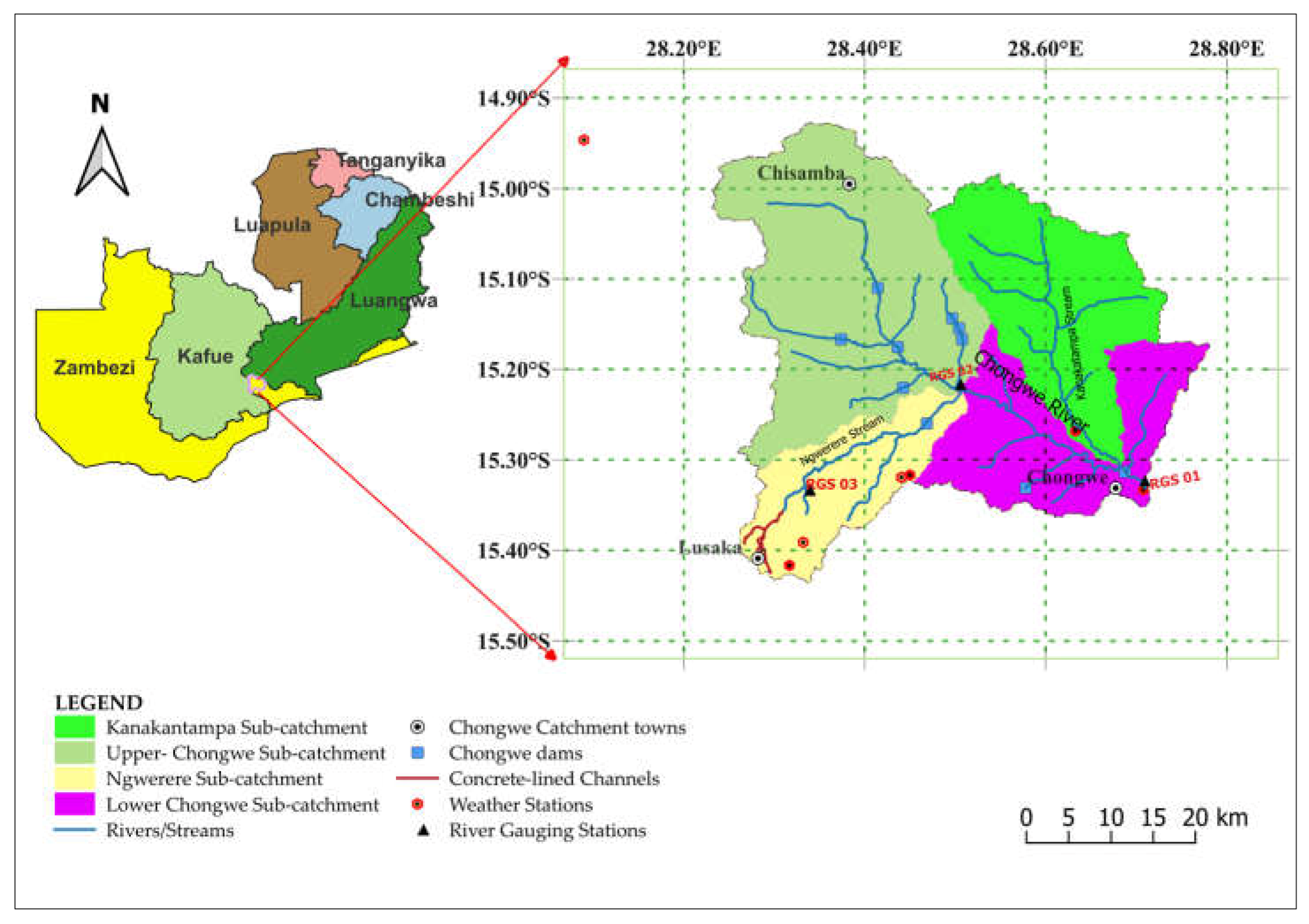
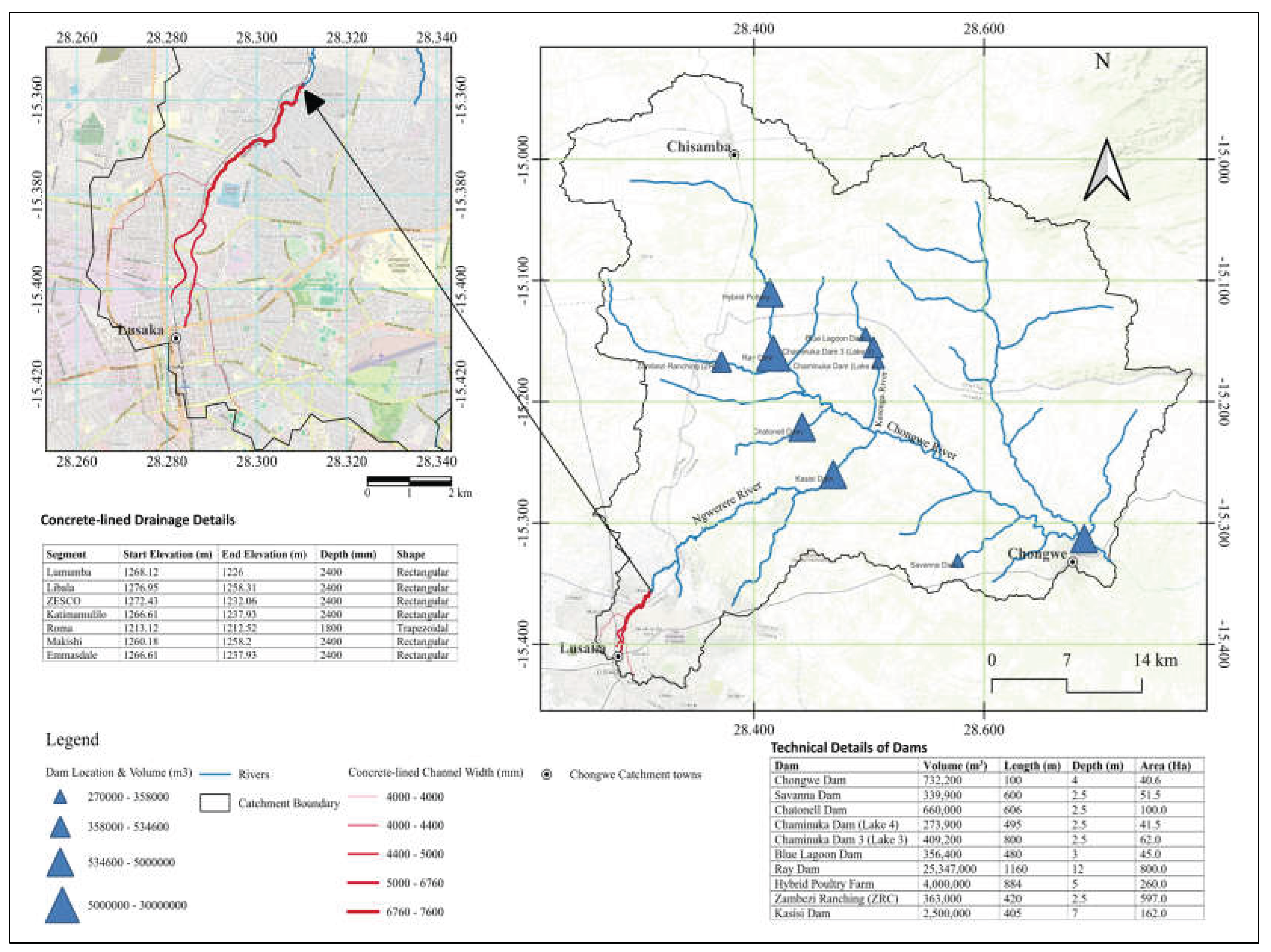
Figure 1.
Location of the Chongwe River Catchment in Zambia showing sub-catchments, drainage features including rivers, concrete-lined channels and dams, as well as the locations of weather stations, river gauging stations and major towns.
Figure 1.
Location of the Chongwe River Catchment in Zambia showing sub-catchments, drainage features including rivers, concrete-lined channels and dams, as well as the locations of weather stations, river gauging stations and major towns.
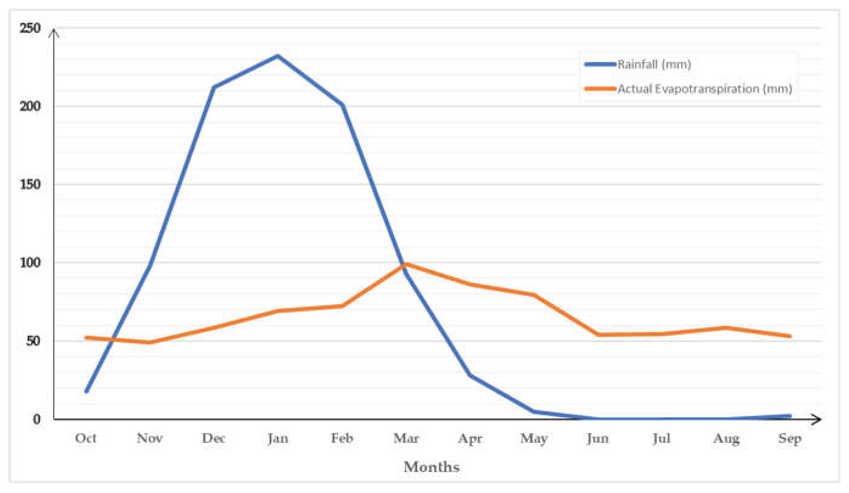
Figure 2.
Averaged monthly rainfall (mm) and actual evapotranspiration (mm) of Chongwe Catchment.
Figure 2.
Averaged monthly rainfall (mm) and actual evapotranspiration (mm) of Chongwe Catchment.
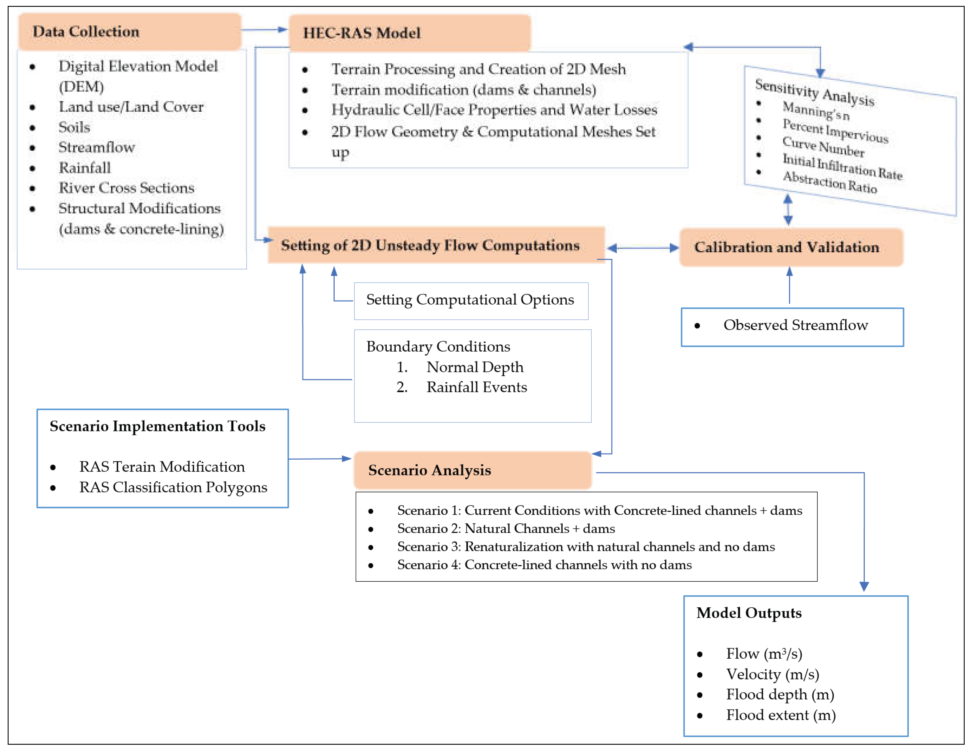
Figure 3.
Overall Methodological Approach of the study.
Figure 3.
Overall Methodological Approach of the study.
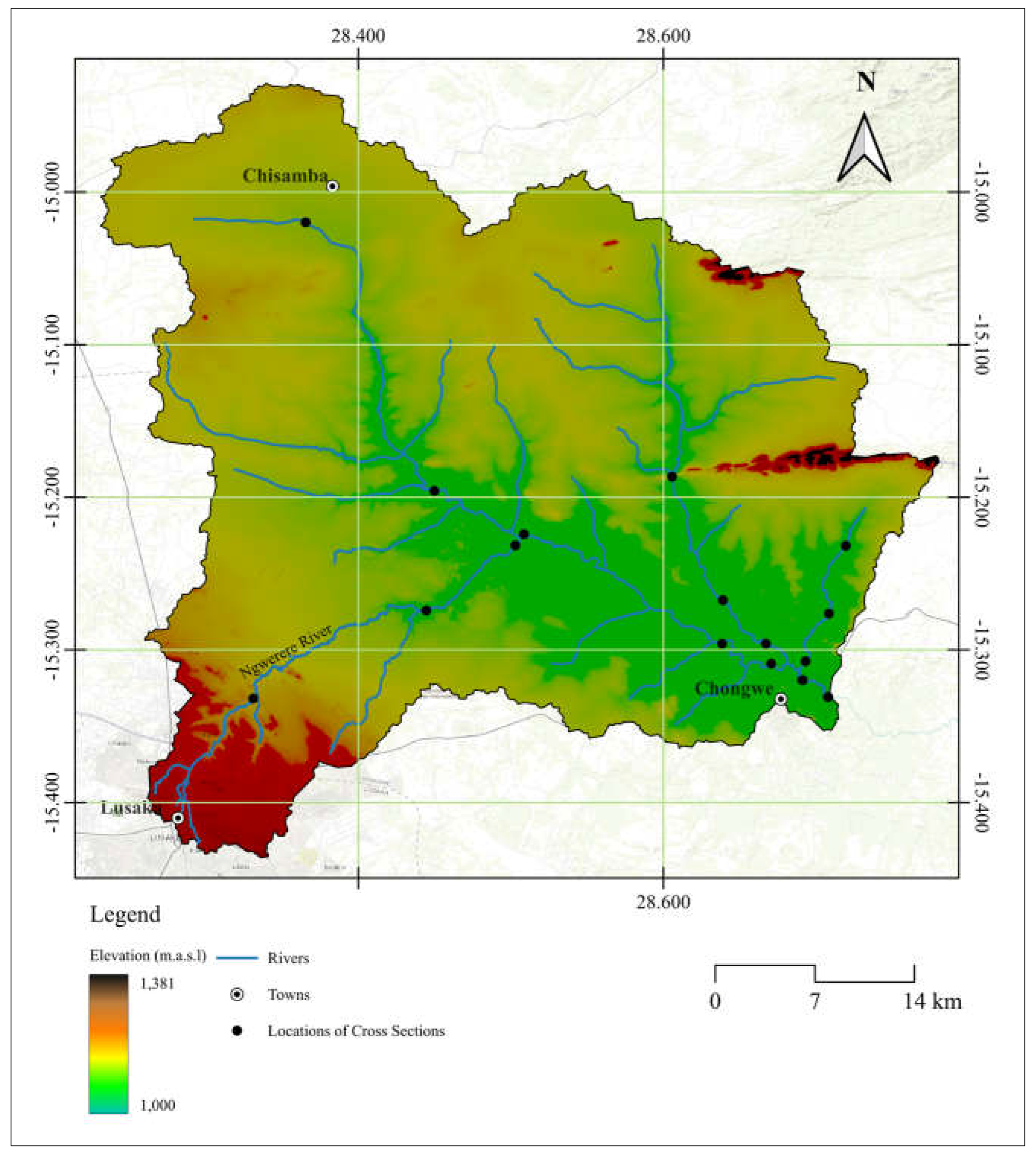
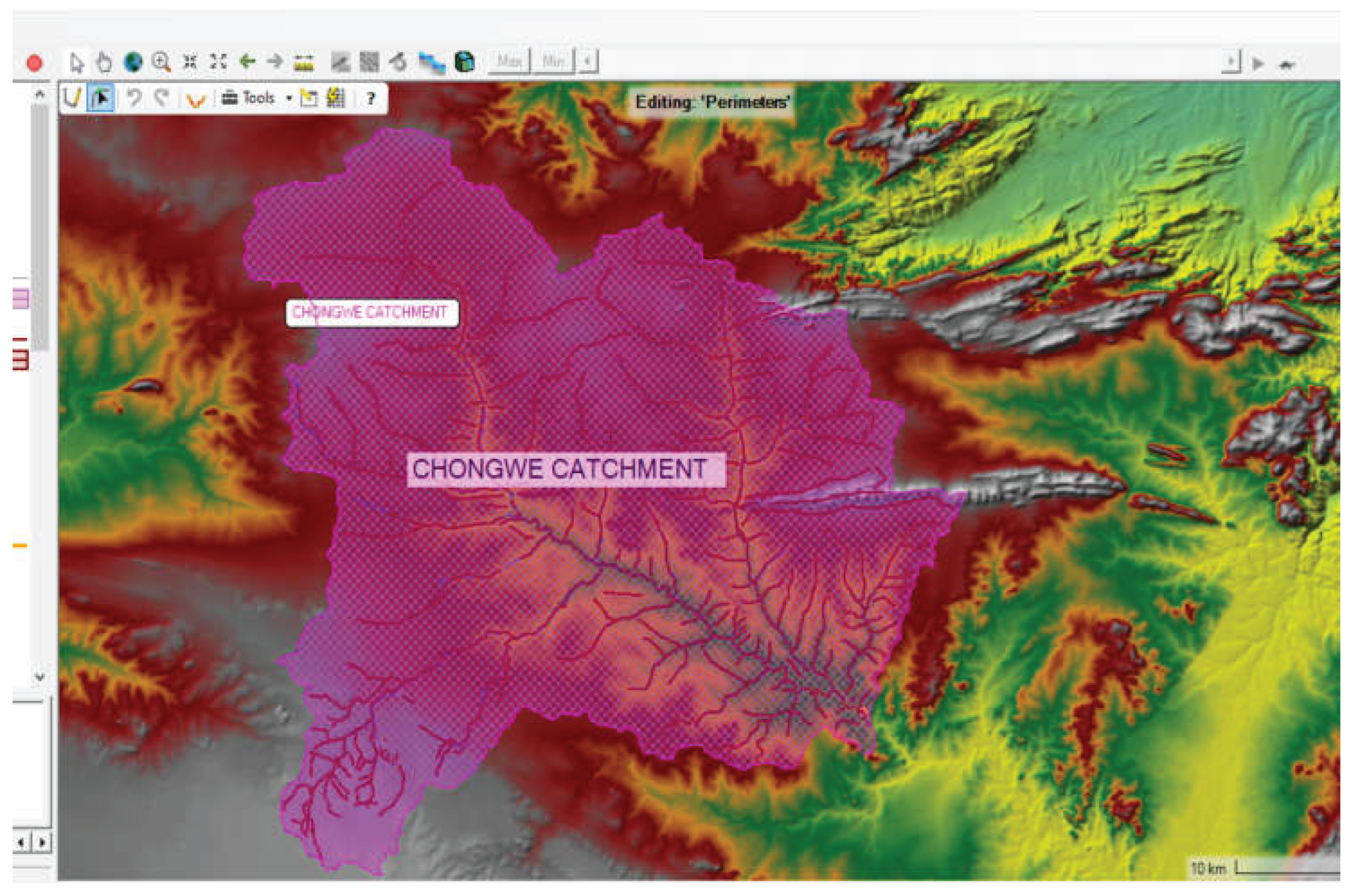
Figure 4.
Digital Elevation Model and Location of Cross Sections.
Figure 4.
Digital Elevation Model and Location of Cross Sections.
Figure 5.
Location and details of the concrete-lined channel and existing dams.
Figure 5.
Location and details of the concrete-lined channel and existing dams.
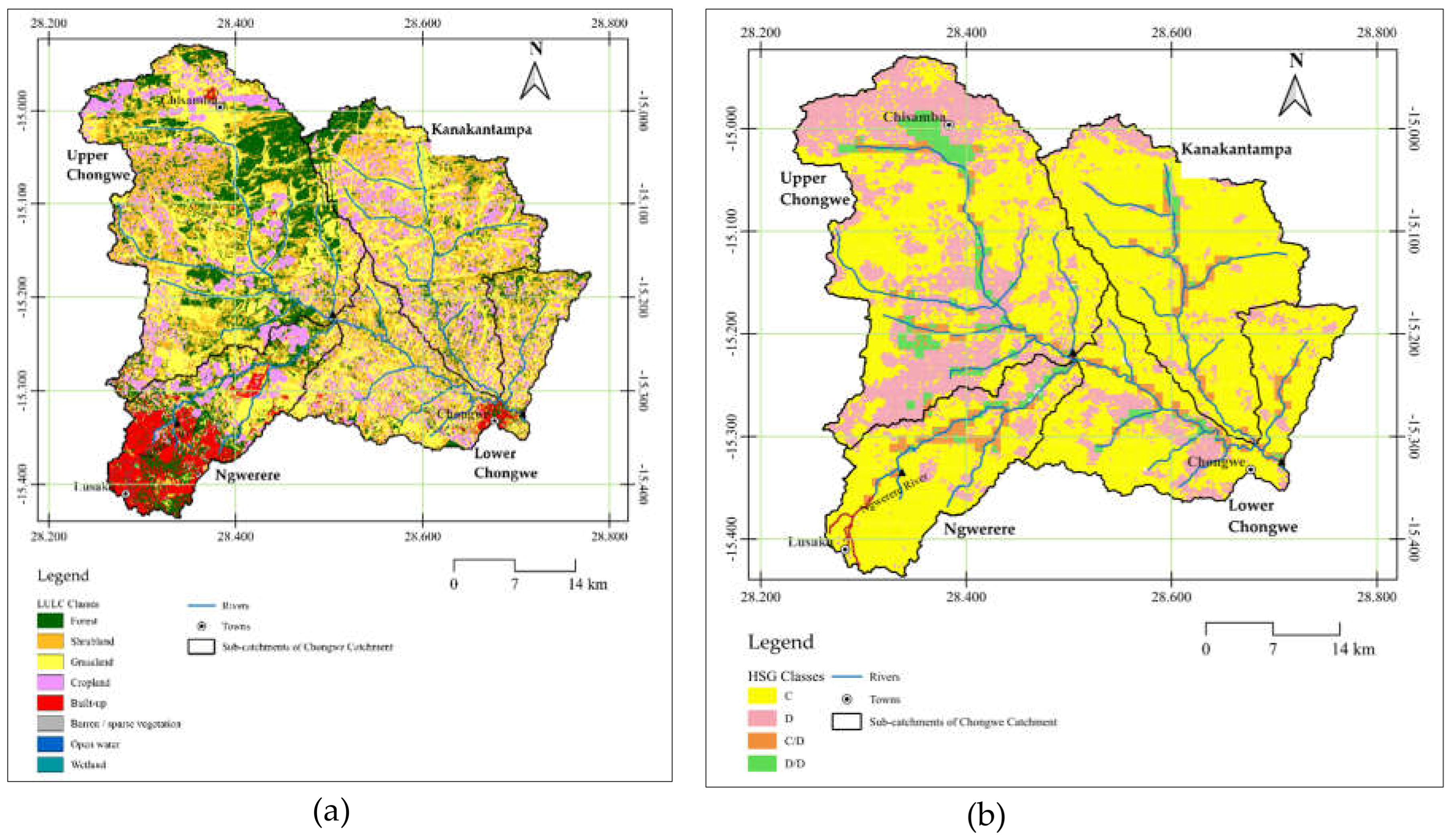
Figure 6.
(a) LULC map of the Catchment; (b) Hydrological Soil Groups (HSGs) of the Catchment.
Figure 6.
(a) LULC map of the Catchment; (b) Hydrological Soil Groups (HSGs) of the Catchment.
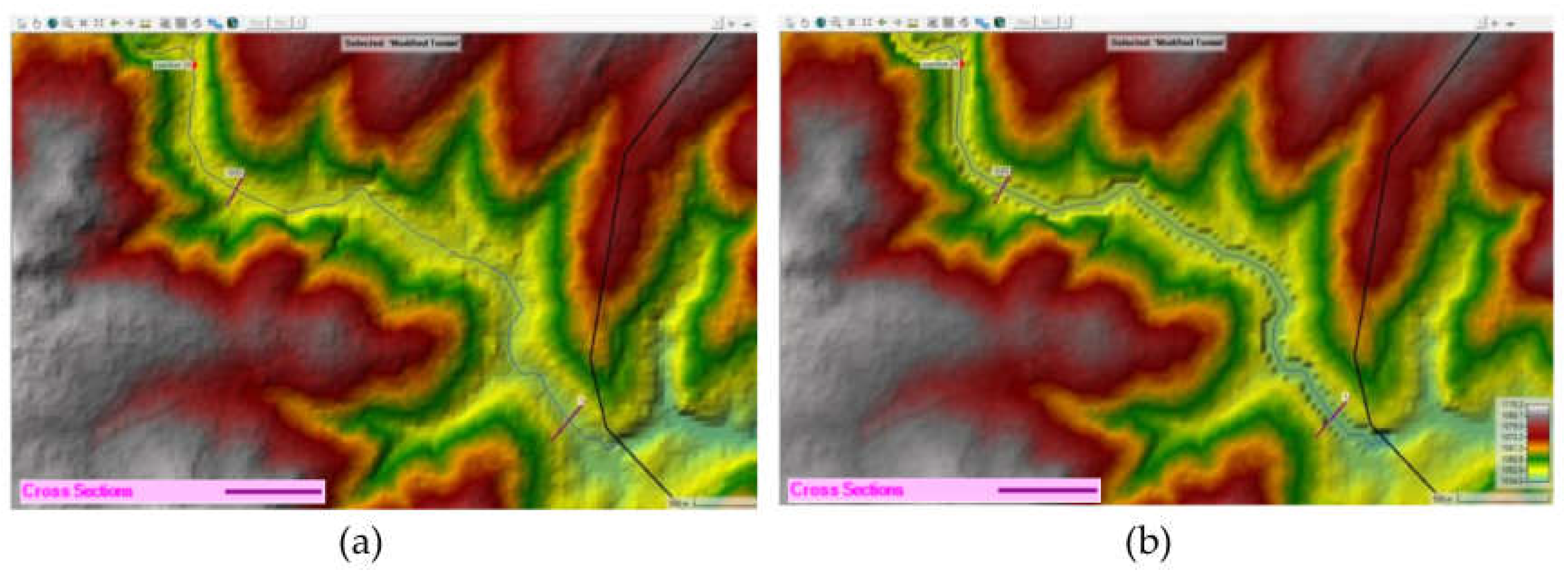
Figure 7.
(a) Original terrain model; (b) Modified terrain model.
Figure 7.
(a) Original terrain model; (b) Modified terrain model.
Figure 8.
Developed computational mesh for 2D Flow Area (Red lines indicate breaklines; Background is the terrain model).
Figure 8.
Developed computational mesh for 2D Flow Area (Red lines indicate breaklines; Background is the terrain model).
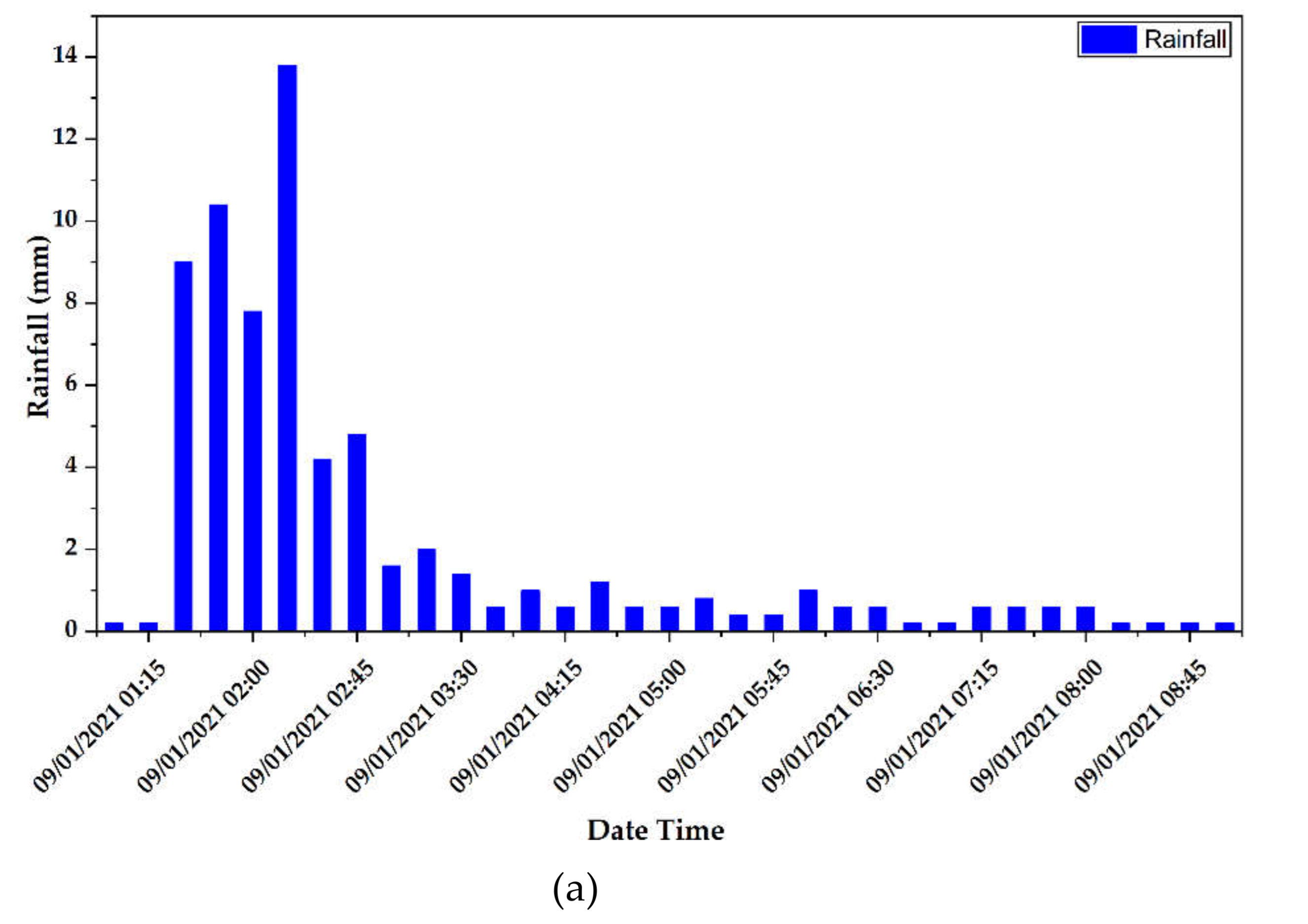
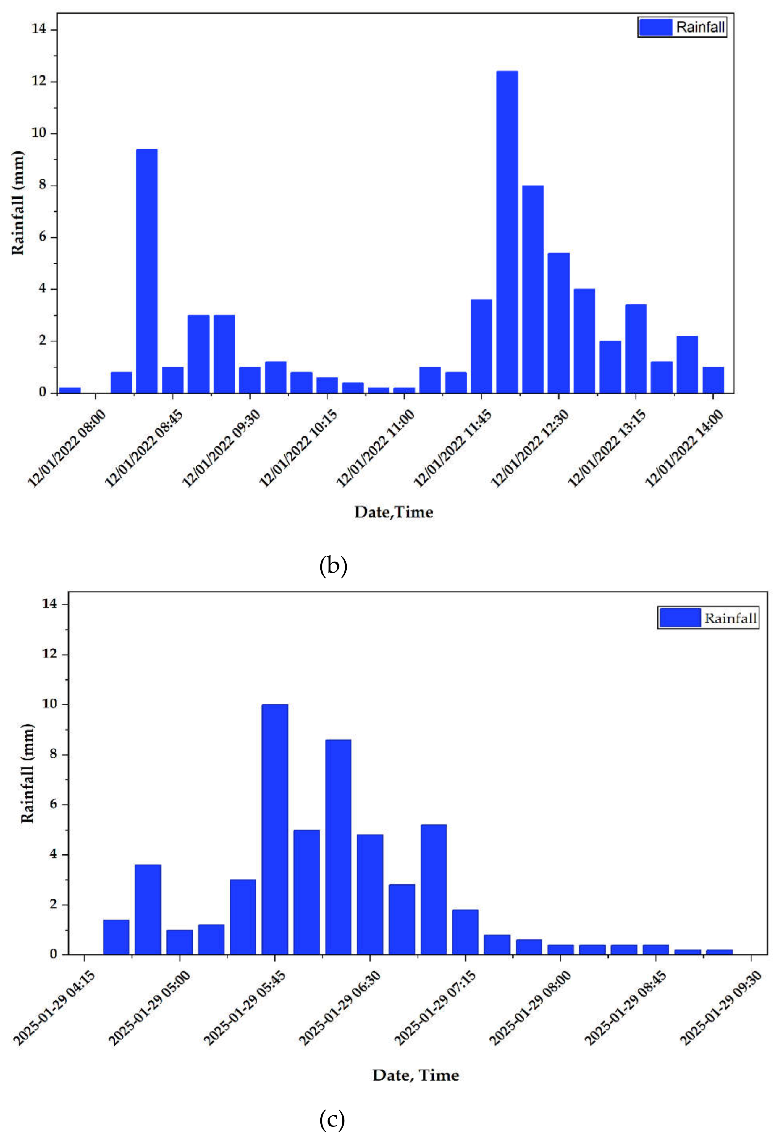
Figure 9.
Rainfall hydrographs for (a) calibration, (b) validation and (c) scenario analysis.
Figure 9.
Rainfall hydrographs for (a) calibration, (b) validation and (c) scenario analysis.
Figure 10.
Sub-hourly (15-min) flow calibration results for gauging station RG1 located at Great East Road Bridge.
Figure 10.
Sub-hourly (15-min) flow calibration results for gauging station RG1 located at Great East Road Bridge.
Figure 11.
Sub-hourly (15-min) flow validation results for gauging station RG1 located at Great East Road Bridge.
Figure 11.
Sub-hourly (15-min) flow validation results for gauging station RG1 located at Great East Road Bridge.
Figure 12.
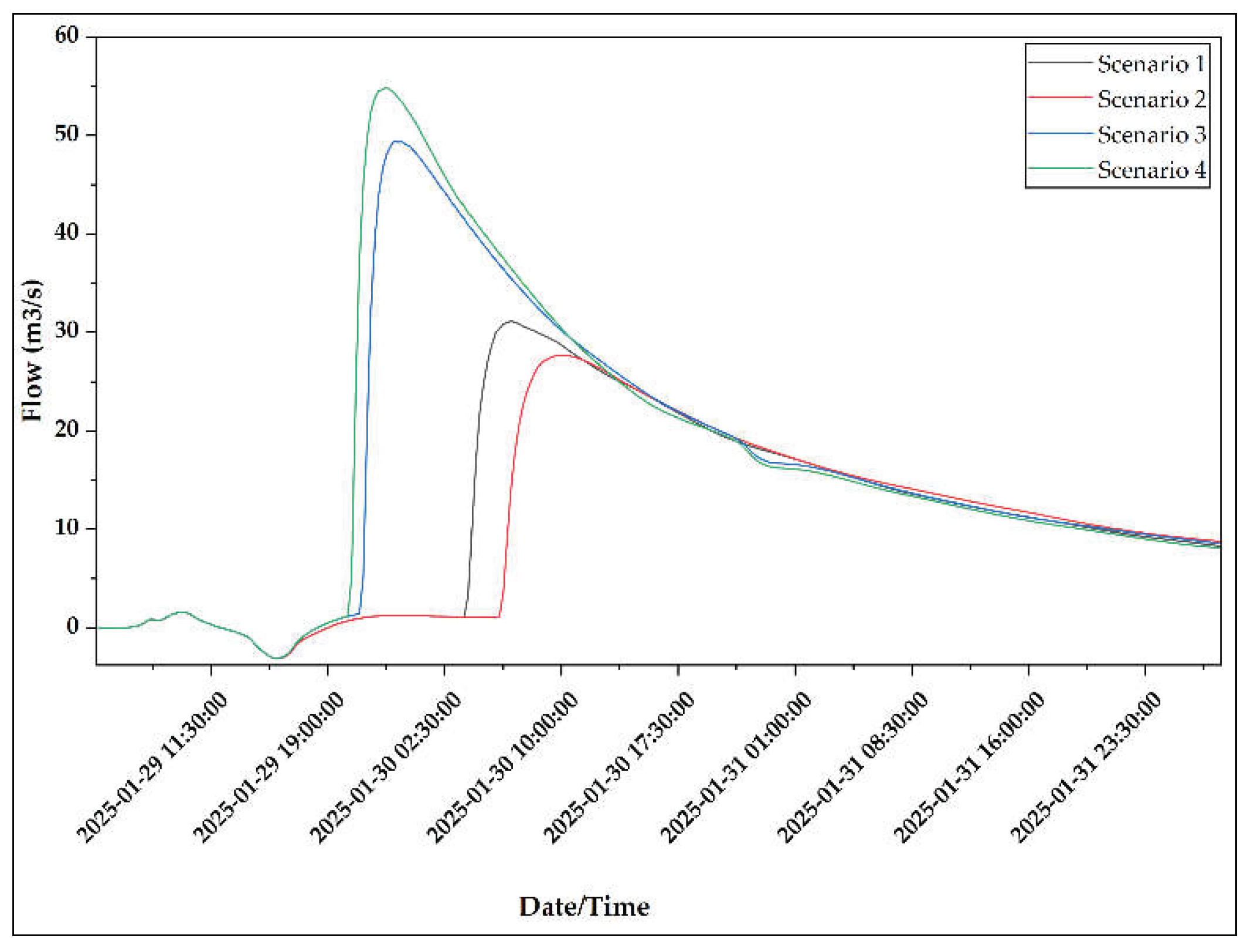
High flow characteristics at the Ngwerere outlet for different scenarios.
Figure 12.
High flow characteristics at the Ngwerere outlet for different scenarios.
Figure 13.
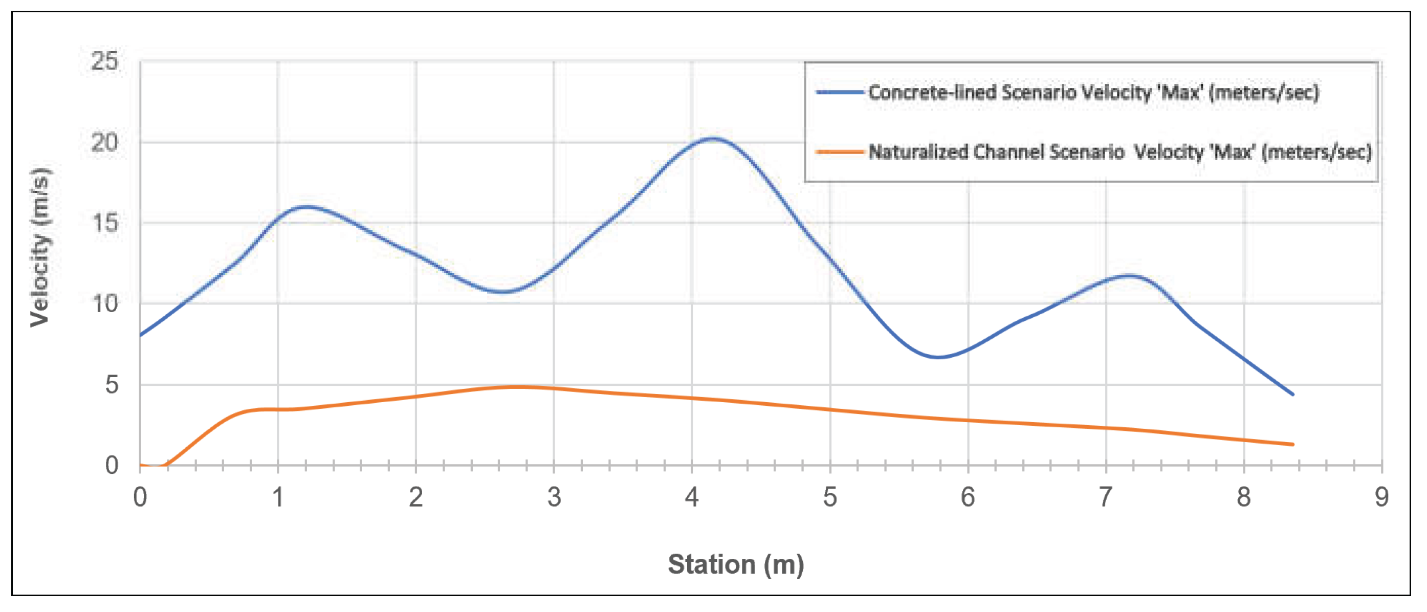
Comparison of velocity in a naturalized channel and a concrete-lined channel at Kasangula Road Bridge (KRB).
Figure 13.
Comparison of velocity in a naturalized channel and a concrete-lined channel at Kasangula Road Bridge (KRB).
Figure 14.
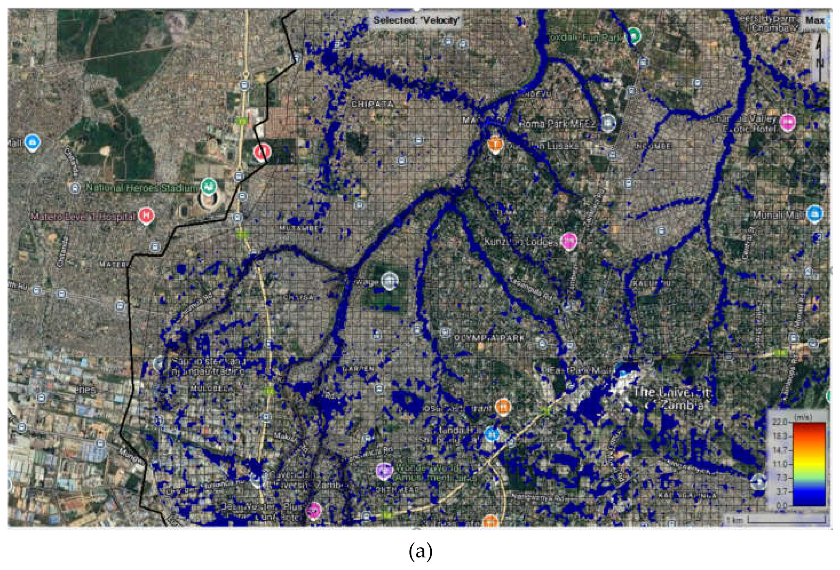
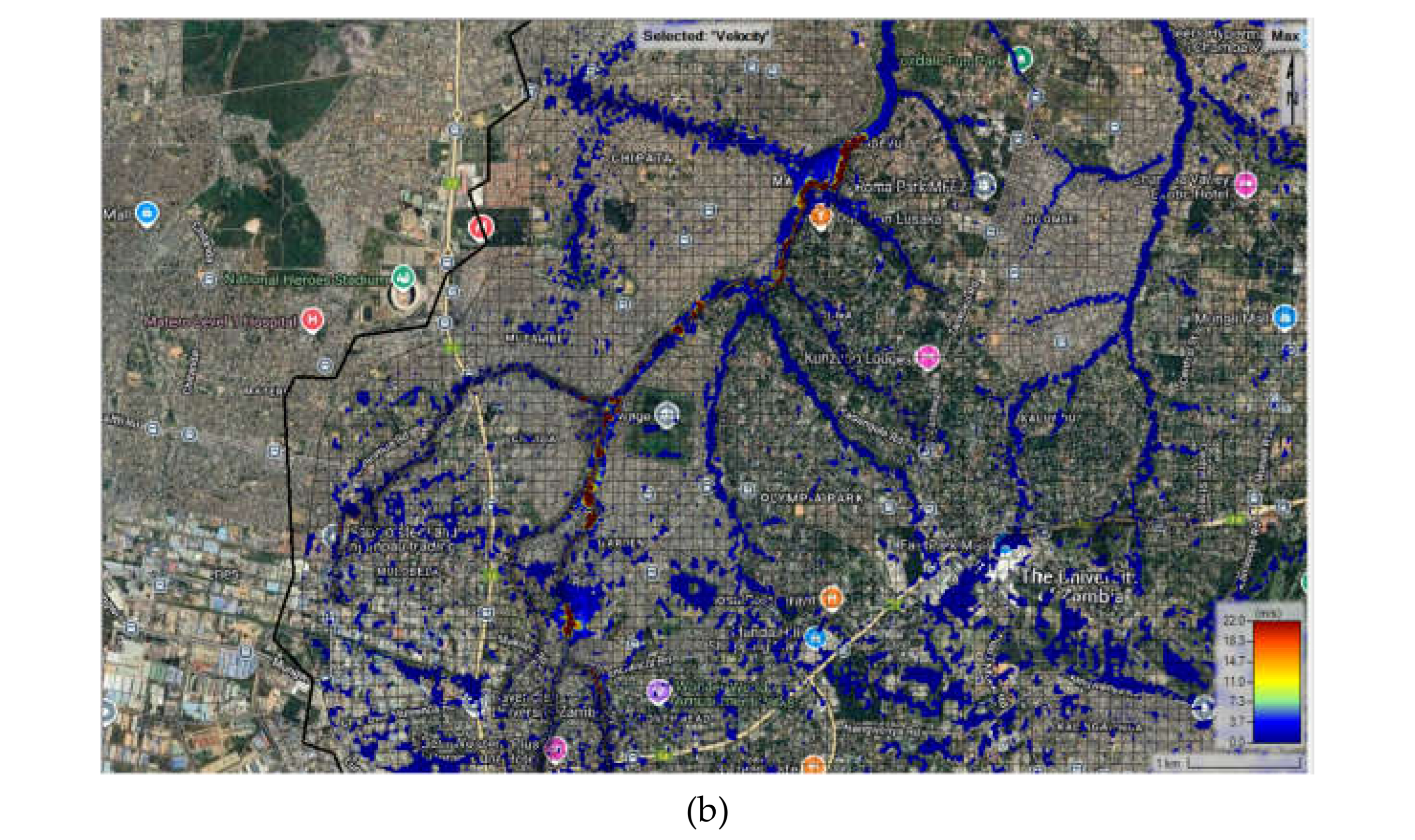
Comparison of maximum velocities along: (a) Naturalized channel (Scenario 3) and (b) Concrete-lined channel (Scenario 4) in Lusaka.
Figure 14.
Comparison of maximum velocities along: (a) Naturalized channel (Scenario 3) and (b) Concrete-lined channel (Scenario 4) in Lusaka.
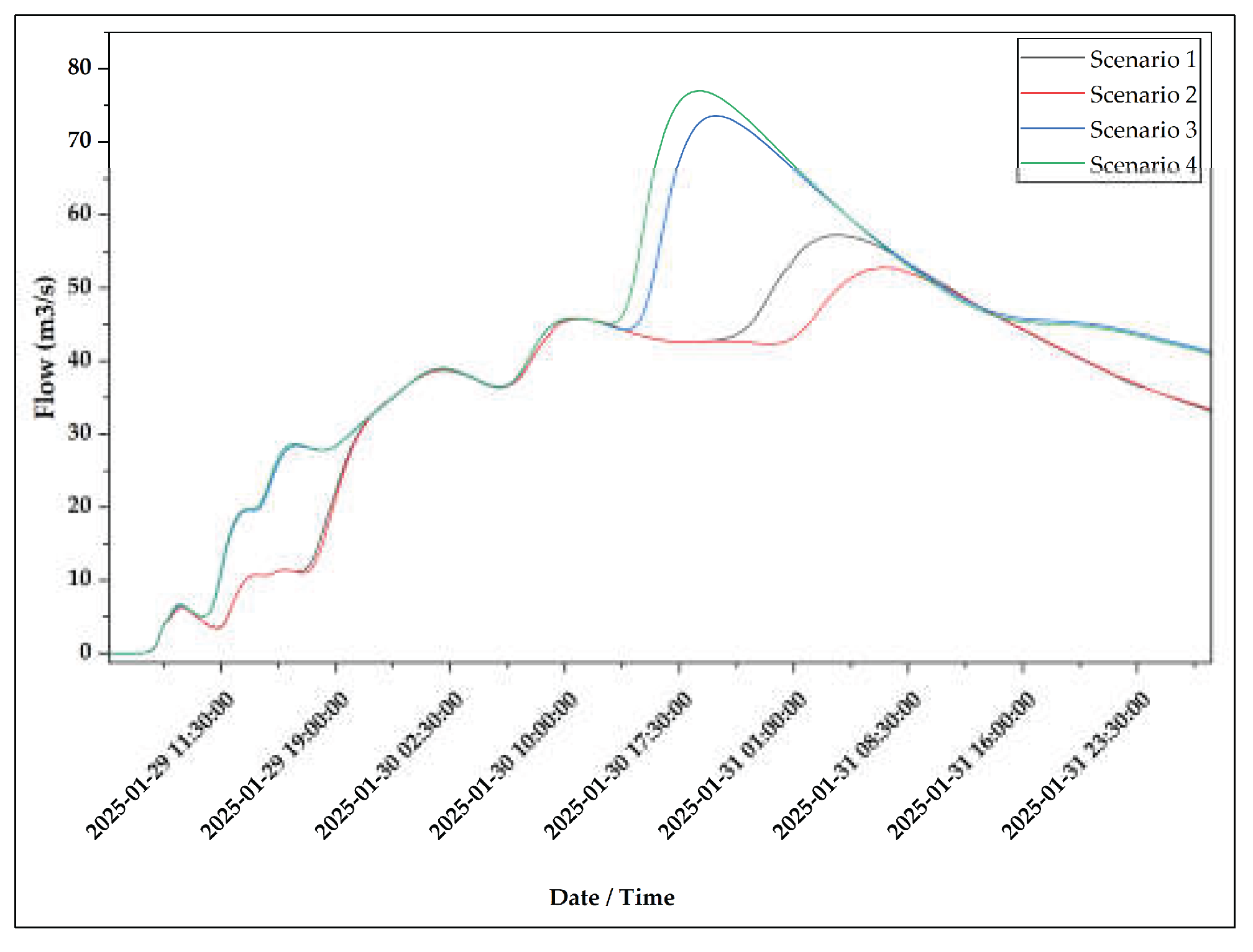
Figure 15.
Summary of Flow Characteristics at Chongwe main outlet for the four scenarios.
Figure 15.
Summary of Flow Characteristics at Chongwe main outlet for the four scenarios.
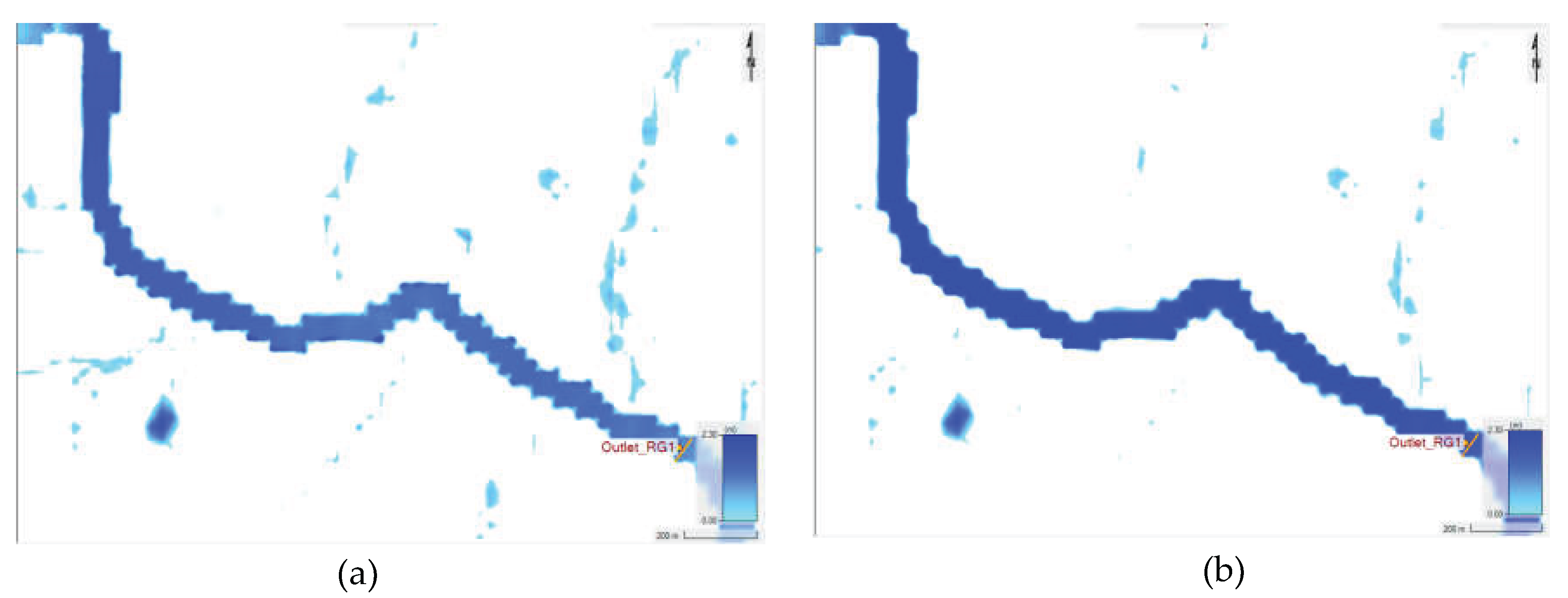
Figure 16.
Comparison of maximum flood depth distribution in RAS Mapper at the Chongwe River (RG1) Reach under (a) natural channel conditions without concrete-lining (Scenario 3) and (b) concrete-lined channel conditions in Lusaka City (Scenario 4).
Figure 16.
Comparison of maximum flood depth distribution in RAS Mapper at the Chongwe River (RG1) Reach under (a) natural channel conditions without concrete-lining (Scenario 3) and (b) concrete-lined channel conditions in Lusaka City (Scenario 4).
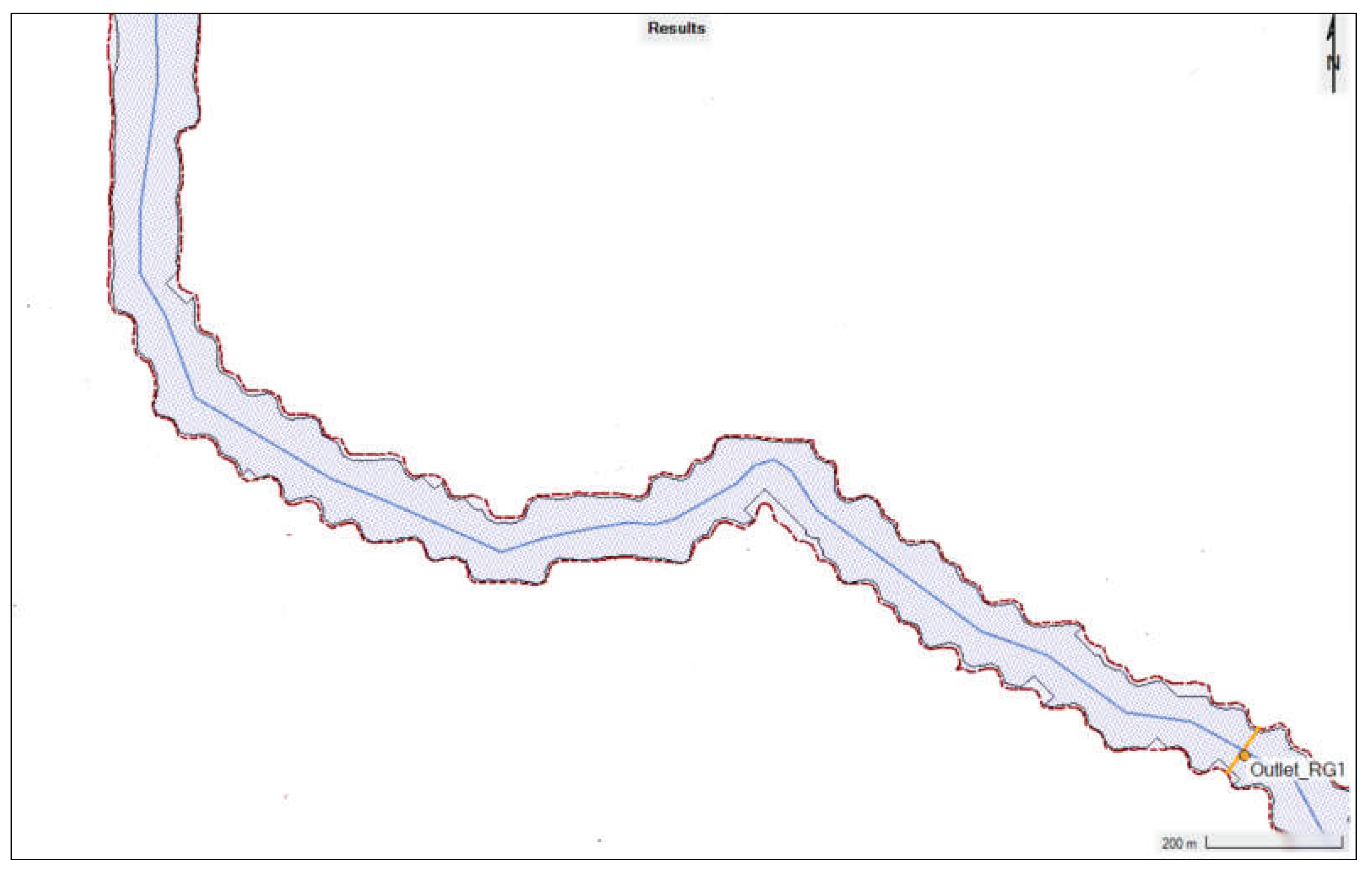
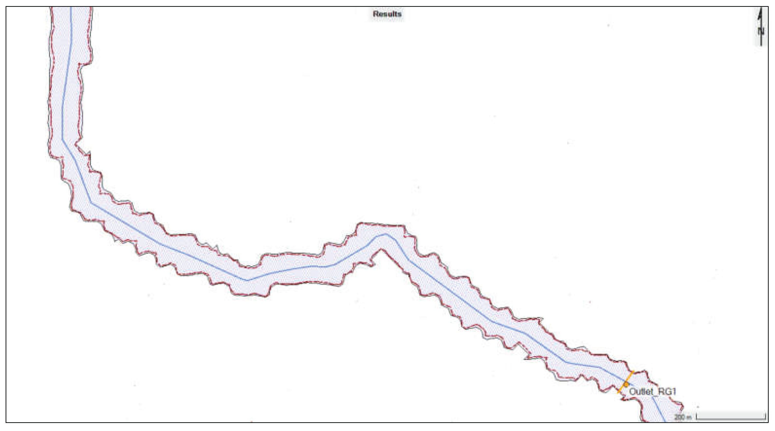
Figure 17.
Overlay comparison of flood inundation boundaries in RAS Mapper at the Chongwe River Outlet (RG1) Reach for Scenario 3 (natural channels, shown by the black solid line) and Scenario 4 (concrete-lined channels, shown by the red dashed line).
Figure 17.
Overlay comparison of flood inundation boundaries in RAS Mapper at the Chongwe River Outlet (RG1) Reach for Scenario 3 (natural channels, shown by the black solid line) and Scenario 4 (concrete-lined channels, shown by the red dashed line).
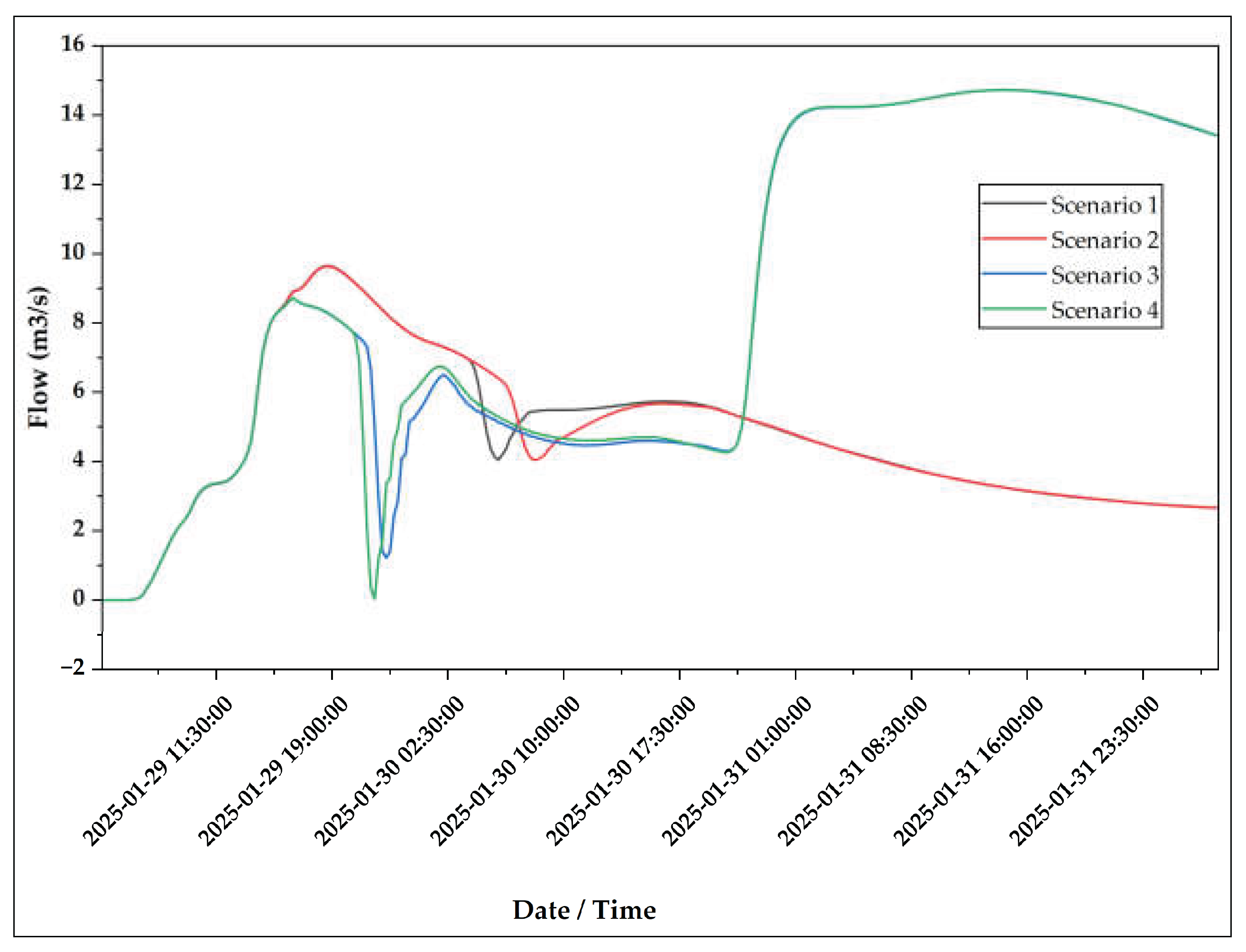
Figure 18.
High flow characteristics at the Upper Chongwe outlet for different scenarios.
Figure 18.
High flow characteristics at the Upper Chongwe outlet for different scenarios.
Figure 19.
Overlay comparison of flood inundation boundaries in RAS Mapper at the Chongwe River (RG1) Reach for Scenario 3 (natural channels, shown by the black solid line) and Scenario 1 (concrete-lined channels with dams shown by the brown dashed line).
Figure 19.
Overlay comparison of flood inundation boundaries in RAS Mapper at the Chongwe River (RG1) Reach for Scenario 3 (natural channels, shown by the black solid line) and Scenario 1 (concrete-lined channels with dams shown by the brown dashed line).
Table 1.
Sub-catchments of the Chongwe River Catchment.
Table 1.
Sub-catchments of the Chongwe River Catchment.
| Sub-Catchment |
Size (km2) |
Predominant Land Use |
| Upper-Chongwe |
809 |
Agriculture, Ranch, Irrigation |
| Ngwerere |
289 |
Built up, Agriculture, Irrigation |
| Kanakantapa |
482 |
Forest, Rainfed Agriculture, Settlements |
| Lower-Chongwe |
384 |
Built-up, Agriculture |
| Total |
1964 |
|
Table 2.
Description of Hydrologic Soil Groups [
42].
Table 2.
Description of Hydrologic Soil Groups [
42].
| HSG |
Description |
| A |
Low runoff potential (>90% sand and <10% clay) |
| B |
Moderately low runoff potential (50–90% sand and 10–20% clay) |
| C |
Moderately high runoff potential (<50% sand and 20–40% clay) |
| D |
High runoff potential (<50% sand and >40% clay) |
| A/D |
High runoff potential unless drained (>90% sand and <10% clay) |
| B/D |
High runoff potential unless drained (50–90% sand and 10–20% clay) |
| C/D |
High runoff potential unless drained (<50% sand and 20–40% clay) |
| D/D |
High runoff potential unless drained (<50% sand and >40% clay) |
Table 3.
Rainfall events for calibration, validation and scenario analysis.
Table 3.
Rainfall events for calibration, validation and scenario analysis.
| Event |
Date |
Start Time
(HH: MM) |
End-Time
(HH: MM) |
Comment |
| 1 |
09 January, 2021 |
01:00 |
09:15 |
Calibration |
| 2 |
12 January, 2022 |
07:45 |
14:00 |
Validation |
| 3 |
29 January, 2025 |
04:30 |
09:15 |
Scenario Analysis |
Table 4.
Classification criteria for hydrological models [
61].
Table 4.
Classification criteria for hydrological models [
61].
| Goodness-of-Fit |
NSE |
PBIAS (%) |
R2
|
| Very Good (V) |
0.75 < NSE ≤ 1.00 |
PBIAS <± 10 |
R2 ≥ 0.75 |
| Good (G) |
0.60 < NSE ≤ 0.75 |
±10 ≤ PBIAS <± 15 |
0.70 < R2 ≤ 0.75 |
| Satisfactory (S) |
0.50 < NSE ≤ 0.60 |
± 15 ≤ PBIAS <± 45 |
0.60 < R2 ≤ 0.75 |
| Unsatisfactory (U) |
NSE ≤ 0.50 |
PBIAS ≥± 45 |
R2 < 0.60 |
Table 5.
Simulated Scenarios.
Table 5.
Simulated Scenarios.
| Scenario |
Name |
Description |
HEC-RAS Action Tool |
| 1 |
Current Conditions (Concrete Channels + Dams) |
Simulating of catchment as it is with existing 21 km concrete-lined channels and 10 dams |
Calibrated model and observed storm |
| 2 |
Natural Channels + Dams |
Simulating the peak flows before concrete-lining of the 21 km of the natural channels in Lusaka, and while observing the effect of dam storage |
Adjusting Manning’s number of the classification polygons assigned to the concrete-lined channels to natural channels |
| 3 |
Renaturalization: Natural Channels + No Dams |
Simulating the catchment under fully naturalized channels, representing a close to undisturbed channel flow response |
Through terrain modification using the channel tool at the dam walls |
| 4 |
Concrete Channels, No Dams |
Simulating a system with concrete-lined channels in Lusaka but without irrigation dams, to highlight the significance of storage in high flow conditions. |
Combination of two actions above (2 & 3) |
Table 6.
Morris (OAT) Sensitivity Analysis Rankings.
Table 6.
Morris (OAT) Sensitivity Analysis Rankings.
| Parameter |
Initial Value (xi) |
Perturbation (Δxi) |
Initial Peak Flow (eb) (m3/s) |
Perturbed Flow (ea) (m3/s) |
Ei (r=1) |
Absolute Effect (μi*) |
Sensitivity Ranking |
| Manning’s n |
0.064 |
0.012 |
122.760 |
105.990 |
−1,397.500 |
1,397.500 |
Very High |
| % Impervious |
16.000 |
3.200 |
122.760 |
145.89 |
+7.230 |
7.230 |
Low |
| Curve Number |
86.310 |
10.090 |
122.760 |
386.400 |
+ 26.140 |
26.140 |
Low |
| Initial Infiltration Rate (mm/hr.) |
1.300 |
0.260 |
122.760 |
117.080 |
−21.850 |
21.850 |
Low |
| Abstraction Ratio |
0.200 |
0.04 |
122.760 |
110.580 |
−30.500 |
30.500 |
Low |
Table 7.
Relative threshold criteria for classifying parameter sensitivity [
59].
Table 7.
Relative threshold criteria for classifying parameter sensitivity [
59].
| μ* Range (Relative to Max) |
Sensitivity Classification |
| μ* > 700 |
Very High |
| 150 < μ* ≤ 700 |
High |
| 50 < μ* ≤ 150 |
Moderate |
| μ* ≤ 50 |
Low |
Table 8.
Initial and calibrated Manning’s n & % impervious values.
Table 8.
Initial and calibrated Manning’s n & % impervious values.
| |
LULC Class |
Manning’s n |
Percent Impervious %) |
| ID |
Name |
Initial |
Calibrated |
Initial |
Calibrated |
| 1 |
Shrubland |
0.100 |
0.120 |
2.000 |
2.000 |
| 3 |
Built-up Land |
0.045 |
0.030 |
70.000 |
85.000 |
| 4 |
Grassland |
0.060 |
0.055 |
5.000 |
5.000 |
| 5 |
Cropland |
0.050 |
0.050 |
2.000 |
3.000 |
| 6 |
Barren Land |
0.040 |
0.030 |
0.000 |
0.000 |
| 7 |
Wetland |
0.120 |
0.120 |
0.000 |
0.000 |
| 8 |
Open Water |
0.025 |
0.025 |
0.000 |
0.000 |
| 10 |
Forest |
0.120 |
0.160 |
1.000 |
1.000 |
| 9 |
Natural Channel |
0.035 |
0.035 |
1.000 |
1.000 |
| 2 |
C* Drain |
0.013 |
0.013 |
1.000 |
100.000 |
Table 9.
Summary of Flow Characteristics at Ngwerere Outlet for the four scenarios.
Table 9.
Summary of Flow Characteristics at Ngwerere Outlet for the four scenarios.
| Scenario |
Peak Flow (m3/s) |
Lag-Time (hr.) |
Maximum Flood Depth (m) |
Flood Extent (m) |
| 1 |
31.14 |
25.00 |
3.44 |
110.00 |
| 2 |
27.72 |
28.15 |
3.37 |
105.00 |
| 3 |
49.44 |
17.30 |
3.79 |
114.00 |
| 4 |
54.91 |
17.50 |
3.88 |
117.00 |
Table 10.
Summary of Flow Characteristics at Chongwe main outlet for the four scenarios.
Table 10.
Summary of Flow Characteristics at Chongwe main outlet for the four scenarios.
| Scenario |
Peak Flow (m3/s) |
Lag-time (hr.) |
Maximum Flood Depth (m) |
Flood extent (m) |
| 1 |
57.25 |
46.00 |
1.81 |
100.00 |
| 2 |
52.82 |
49.25 |
1.77 |
98.00 |
| 3 |
73.60 |
38.25 |
1.99 |
102.00 |
| 4 |
77.00 |
37.00 |
2.22 |
104.00 |
Table 11.
Summary of Flow Characteristics at Upper Chongwe Outlet for the four scenarios.
Table 11.
Summary of Flow Characteristics at Upper Chongwe Outlet for the four scenarios.
| Scenario |
Peak Flow (m3/s) |
Lag-time (hr.) |
Maximum Flood Depth (m) |
Flood extent (m) |
| 1 |
9.65 |
13.00 |
1.15 |
101.00 |
| 2 |
9.64 |
13.00 |
1.11 |
97.00 |
| 3 |
14.73 |
56.45 |
1.50 |
105.00 |
| 4 |
14.74 |
57.00 |
1.59 |
108.00 |