
Submitted:
01 February 2025
Posted:
03 February 2025
You are already at the latest version
Abstract
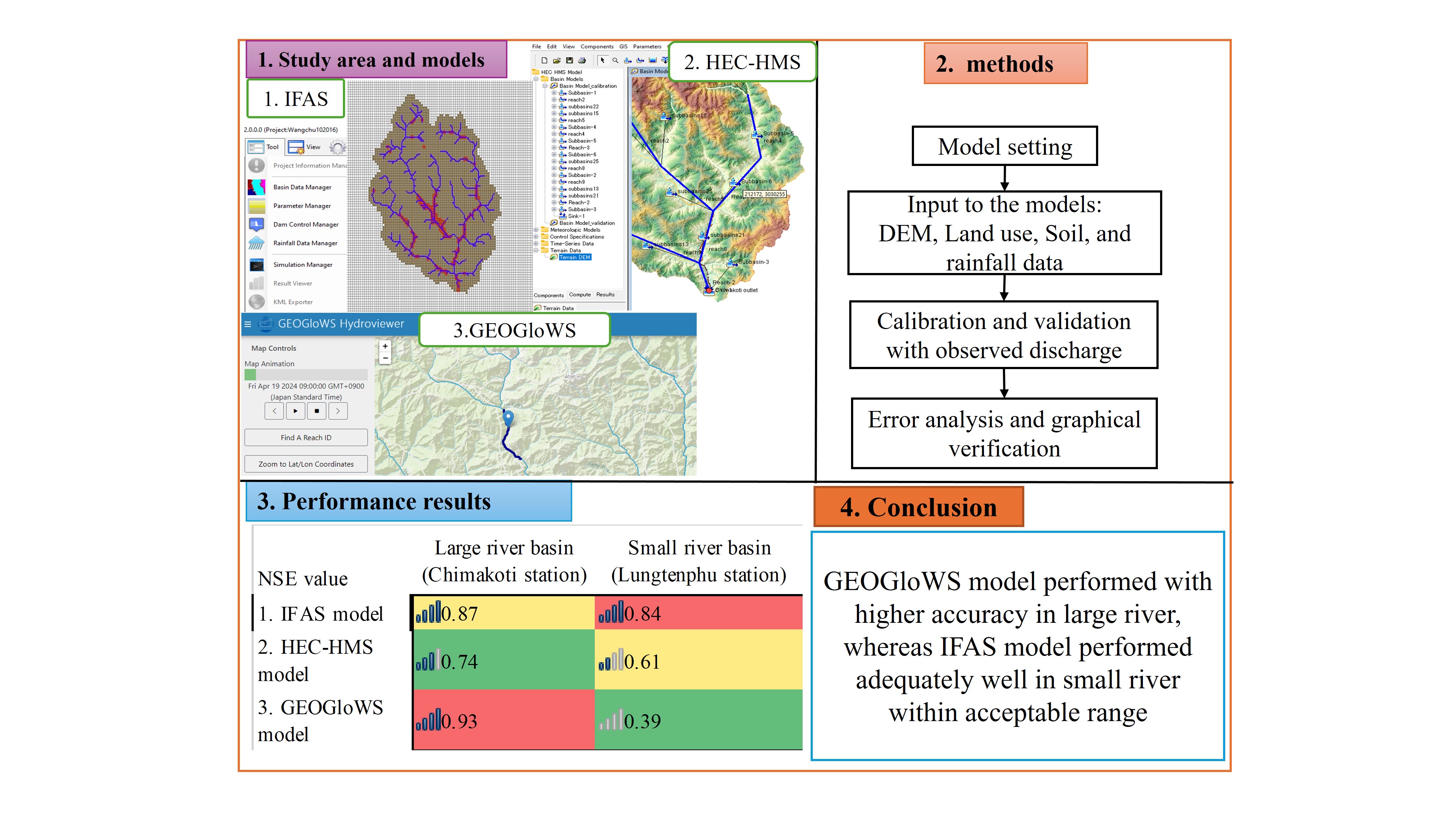
Flood has become a major hazard globally, and Bhutan with its steep terrain and erratic rainfall has caused significant economic damages in recent years. Given these challenges, there is a lack of accurate flood prediction and management strategies. This study, there-fore, evaluates three hydrological models—Integrate Flood Analysis System (IFAS), Hy-drologic Engineering Centre Hydrologic Modeling System (HEC-HMS), and Group on Earth Observation Global Water Sustainability version 1 (GEOGloWS)—and identifies the most suitable model for simulating flood events in Wangchu River Basin of Bhutan. Fur-ther, it also examined the model performance for Large and Small Basins using Nash-Sutcliffe Efficiency (NSE), Percentage Bias (PBIAS) and Peak Flow Error (PFE) met-rics. Overall, the GEOGloWS model demonstrated the highest accuracy in simulating flood in large basin, achieving the NSE, PBIAS and PFE values of 0.93, 3.21 and 4.48, re-spectively. In small basin, the IFAS model showed strong performance with an NSE value of 0.84, although the discharge was underestimated. The GEOGloWS model provides simulated discharge but need to be bias corrected before use. The calibrated parameters can be used in IFAS and HEC-HMS models to simulate flood in Wangchu Basin and adjacent basins having similar geographical characteristics for future studies.
Keywords:
flood simulation
; hydrological models
; model performance
; mountainous region
; Wangchu river basin
1. Introduction
Floods have become increasingly frequent and severe worldwide, largely driven by climate change, which disrupts precipitation patterns and amplifies extreme rainfall events. These changes have already had devastating impacts. For instance, floods claimed over 220,000 lives globally between 1980 and 2013, and in 2017 alone, weather-related disasters caused economic losses exceeding US$300 billion [1,2]. Projections further underscore the escalating risks, with climate change expected to increase population vulnerability to river floods by 20–80% by 2030 and 40–150% by 2080 [1]. The Intergovernmental Panel on Climate Change (IPCC) Sixth Assessment Report forecasts a rise in global mean surface temperature of 1.5℃ to 4℃ above pre-industrial levels by the end of the 21st century [3]. This temperature increase is projected to disrupt precipitation patterns, leading to more extreme rainfall events and heightened flood risks in many river basins [4,5,6] As a result, these changes will have profound impact on lives, livelihoods, economics, and properties worldwide.
Given these escalating risks, there is an urgent need for comprehensive climate change adaptation and disaster risk reduction strategies to mitigate the growing threat of river floods. Regions at particularly high risk according to the IPCC [3] and Nagamani et al. [6], include South Asia, Sub-Sahara Africa and parts of Latin America. These areas are expected to experience some of the most severe impacts, highlighting the need for immediate and targeted action.
In South Asia, Bhutan is particularly vulnerable to severe flood hazards due to a combination of fragile landscape factors. The country’s rugged terrain, with steep slopes and narrow river valleys, along with its location in the path of the seasonal monsoon system, makes it highly susceptible to flood events [7,8]. Climate-induced changes further exacerbate this vulnerability, leading to significant impacts on the hydrological system.
Over the past several decades, Bhutan has experienced recurrent devastating floods, with major events recorded in 1950, 1956, 1960, 1968, 1994, 2000, 2004, 2009, 2016 and most recently in 2023 [8,9]. These flood events have resulted in significant loss of life, livelihoods, and historical monuments. Projections indicate that river discharge in the region will change annually, with annual rainfall expected to increase by 12.1% by 2050 and 27.1% by 2099 [10,11,12]. Notably, Syldon et al. [12] have identified the Wangchu River Basin (WRB) as a highly vulnerable region in Bhutan, where river inundation could increase by up to 60%, posing a severe threat to low-lying agricultural land.
Given the growing frequency and severity of floods, timely implementation of flood warnings and advanced hydrological modeling techniques have become crucial to mitigate the substantial damages [13,14]. Flood mitigation can be most effective by combining structural measures, non-structural measures, and institutions capacity [15,16]. However, in Bhutan’s mountainous terrain, structural measures such as discharge stage and cable system become impractical during high flood events. In this context, flood simulation can be approached through software-based hydrological models (a non-structural measure), which allows for more accurate river discharge estimation at various segments, irrespective of the timing and magnitude of flood events [16]
Developed countries have made significant advancements in predicting floods by employing advanced hydrological models. For instance, the USA has developed models like Hydrologic Engineering Centre – Hydrologic Modeling System (HEC-HMS), Soil and Water Assessment Tool (SWAT) and National Water Model (NWM) [13], while the European Commission created the Global Flood Awareness System (GloFAS) for global flood forecasting [17,18]. In contrast, developing countries, including Bhutan, face significant challenges in flood prediction due to data deficiencies, financial constraints, technical limitations, and lack of tailored flood forecasting models [13], resulting in increased vulnerability and uncertainty in flood prediction and response [19,20].
In Bhutan, the lack of monitoring in small and medium-sized rivers exacerbates flood prediction uncertainties, making it critical to select appropriate models for accurate simulations. Various hydrological models have been employed in Asia, with the Integrated Flood Analysis System (IFAS) providing particularly advantageous for countries such as developing and data-scarce regions like Bhutan [21,22]. IFAS has been used in Japan, Vietnam, Malaysia, the Philippines, Myanmar and Bhutan [23,24,25,26,27,28], showing promising results. The model’s integration of satellite rainfall data, Digital Elevation Models (DEM), and other geographical datasets makes it ideal for flood simulation in remote areas.
Similarly, the HEC-HMS model, although globally recognized, has seen limited use in Bhutan’s mountainous river basins [14,29,30,31]. Dorji et al. [32] and Fakhruddin [19] employed the model for flood simulation in river basins of Bhutan, however, more research is needed to explore its application in these challenging terrains.
Additionally, the development of Group on Earth Observation Global Water Sustainability (GEOGloWS) model, offering global historical discharge data and daily forecasts for around one million sub-basins worldwide [33], has demonstrated high accuracy in flood simulation across various countries like Australia, Brazil, Colombia, the Dominican Republic, Nepal and Peru [18,34]. Despite its success elsewhere, it is yet to be applied in Bhutan, indicating the need for comprehensively evaluation of each model for enhanced flood forecasting and risk management in Bhutan.
While the use of hydrological models in large basins is widespread, systematic evaluation of their relative efficiencies and advancement remain limited [14,16,22,29]. These models have primarily been employed for long-term discharge simulation, fewer studies focusing on flood event simulation. Furthermore, the lack of comparative studies and data in small basin presents a considerable challenge, particularly in regions like Bhutan where small rivers and streams are poorly monitored. To address these gaps, this study evaluates three hydrological models—IFAS, HEC-HMS and GEOGloWS—focusing on their suitability for simulating discharge during flood events in Wangchu and Thimchu river basins of Bhutan. Additionally, the study examines whether model performance varies between the area of 3556km2 and 658.86km2, respectively, using key performance metrics such as Nash-Sutcliffe Efficiency (NSE), Percentage Bias (PBIAS) and Peak Flow Error (PFE) metrics. The findings of this research will provide crucial insights for flood forecasting and risk management, thereby enhancing disaster preparedness in the face of increasing flood risks.
2. Materials and Methods
2.1. Study Area Description
This study focused on Bhutan, a small mountainous kingdom nestled between India and China. Specifically, we examine the upper Wangchu River Basin (WRB) in Western Bhutan, a densly populated region with 240,012 inhabitants and two economically important hydropower plants (Tala - 1020MW and Chhukha - 336MW) [11,35]. The comparative analysis was conducted in WRB (3,556 km²) and the Thimphu River Basin (TRB, 658.86 km²), as illustrated in Figure 1. The WRB is also known as Large River Basin (LRB) while the TRB is referred to as Small River Basin (SRB). Geographically, the area spans three distinct agro-ecological zones: alpine (3,500-7,500 m), cool temperate (2,600-3,600 m), and warm temperate (1,800-2,600 m) [12]. The basin experiences an annual average temperature of 13.4°C and an average of rainfall of 575.1mm/month in July and August. Flow measurements at the Chimakoti station (WRB) from 2001 to 2010 revealed seasonal variations in river discharge, with the highest flow of 251 m³/s occurring in August and the lowest of 26 m³/s in January [35].
2.2. Research Flow
Figure 2 illustrated the research methodology, encompassing the models setup, simulation, calibration, and validation stages for three hydrological models: IFAS, HEC-HMS and GEOGloWS. While IFAS and HEC-HMS models require extensive preprocessing of datasets from satellite and observation stations, the GEOGloWS model offers a more streamlined approach through its pre-developed package. The GEOGloWS model is freely available and provides immediate access through a user-friendly web-service interface. All three models use global data sets to address local data limitations. Models performance were evaluated using three commonly employed performance metrics: NSE, PBIAS and PFE metrics [36,37,38].
2.3. Data Preparation
In three hydrological models, we selected observed river discharge from two distinct flood events for calibration. The calibration period spanned from May 15th to June 14th, 2014, while the validation period covered October 1st to October 31st, 2021. These periods were specifically chosen to coincide with notable flood events, providing a robust foundation for model calibration and validation. For both the IFAS and HEC-HMS models, we employed rainfall data corresponding to these same time frames, as rainfall data serves as a crucial input parameter that directly influences flow patterns within the catchment area. The observed discharge and rainfall data, archived by National Centre for Meteorology and Hydrology (NCHM), Bhutan were used in these models. Daily rainfall data from six meteorological stations and discharge data from two hydrological stations were utilized in this study (Table 1).
For the GEOGloWS model, a minimum of one-year daily observed data is required for bias correction of simulated data at the respective hydrological station (Lozano et al., 2025). For this purpose, observed discharge from 1st January to 31st December, 2021 was used in the model. The bias corrected discharge was extracted from 1st to 31st October, 2021 enabling direct comparison with the validation results from the IFAS and HEC-HMS models.
2.4. Description and Parameter Setting Selected Model
2.4.1. IFAS Model
The IFAS model, developed by the International Centre for Water Hazard and Risk Management (ICHARM), Japan, is freely available and can be downloaded from https://www.pwri.go.jp/icharm/research/ifas/index.html. It serves the rainfall-runoff simulation model designed for the efficient computation of discharge and flood forecasting especially in ungauged river basins [4,39]. The model works based on the principle of tank model for flood simulation and kinematic wave model for routing [26,40]. The model need an input data of DEM, land-use, soil data, and ground and satellite rainfall (Table 2 and Figure S1). Additionally, it features Geographic Information System functionality for the automatic generation of catchment boundary, river channel network, sub-basins, default baseline parameters, and import of boundary river basin.
In this study, as presented in Figure 2, the DEM, land-use, soil, and rainfall data were imported in the model from project information manager tool. The observed rainfall data was prepared in .csv file format and forced in the IFAS model. Then, the IFAS model converted rainfall data to discharge. Two-layer tank model was selected in this study as recommended in the previous studies [21,23]. River discharge was calculated from river course tank model based on Manning’s equation and Kinematic wave method [40]. The input parameters for river course tank model include the breadth of the river course, coefficient of the resume law, Manning’s roughness coefficient, initial water level in the river course, infiltration from river tank to the aquifer tank, and coefficient for cross section shape.
The IFAS model has an automatic function to generate default parameters. Default parameters were used for the initial simulation, however, it failed to synchronize with observed discharge pattern. Therefore, the parameters were calibrated accordingly to align simulated discharge with observed discharge using trial and error method manually. Table S1, S2 and S3 shows all the initial parameters of surface, aquifer and river course tank.
We incorporated all 28 model parameters during the simulation process. However, 5 sensitive parameters were calibrated based on recommendation of the previous studies in the regional studies [16,41]. Notably, parameters were not calibrated separately for SRB, as it falls with the LRB. These identified parameters were also suggested to apply in river basins of Bhutan having similar topography as highlighted in reports and seminar of NCHM, Bhutan.
The parameters such as Final Infiltration Capacity (SKF) and Surface Runoff Coefficient (SNF) values were increased in this model to capture the high flow. The Runoff of confined aquifers (AGD) and Runoff of confined aquifers (AUD) parameter values were reduced to capture low flow (Table 3). The parameters were calibrated carefully to reproduce flow dynamics within the acceptable range. The coefficient for cross section parameter was not calibrated because the simulated high flow aligned with the observed flow. Overall, the simulation with calibrated parameters demonstrated good synchronization with observed river discharge.
2.4.2. Description and Processing of HEC-HMS Model
The HEC-HMS model, developed by the US Army Corps of Engineers, is a physically based semi-distributed rainfall-runoff model used for simulating discharge in dendritic watersheds [29]. The model is widely recognized for its accuracy and extensive use for both event-based and continuous discharge simulations. The primary inputs to the model are precipitation, DEM, Land-use and soil type. We used Alaska Satellite Facility radio-metrically corrected terrain 12.5 resolution Advanced Land Observing Satellite Phased Array type L-band Synthetic Aperture Radar DEM to create subbasins and its characteristics. The DEM was downloaded from https://search.asf.alaska.edu/#/. The soil data with the resolution of 250m was downloaded from https://wocatapps.users.earthengine.app/view/dss-bhutan. The land-use type data of 2016 prepared by National Land Commission of Bhutan was used.
In this study, the river flow was simulated using different meta-models and methods of HEC-HMS such as (1) loss model (Soil Conservation Service Curve Number (SCS-CN)), (2) transform model (SCS Unit hydrograph (SCS-UH)) and (3) routing model (Muskingum). Detailed explanations and processing approaches are explained subsequently.
- Loss model
The SCS-CN method was used to estimate runoff from the catchment [42,43,44]. The method was chosen for its versatility and wide applicability in estimating surface runoff from each subbasins, utilizing equation 1, 2, 3, and 4 [45]. This method required data such as CNs, initial abstraction, and percentage imperviousness of the basin. For this, CNs was prepared in ArcGIS 10.8 with HEC-GeoHMS extension tool using land-use and hydrologic soil group (HSG). The raster data were converted to polygon and created union raster file. The SCS lookup table was created (Table S4) to assign CNs to land-use and HSG following the Technical Report - 55 standard and the NRCS (Natural Resources Conservation Service) land-use table [46]. The equations 1 to 7 compute parameters such as average CNs, accumulated precipitation, maximum retention potential, Time of Concentration ()and Lag time (). The curve number was calculated using the following equation.
where, is the number of sub-basin, Ai is the area of the particular sub-basin and is the total area of the basin.
The accumulated excess precipitation is calculated by equation 2
where is accumulated precipitation excess, unaccumulated rainfall depth, Ia is the initial abstraction and S is maximum retention potential.
The is calculated by equation 3.
And is calculated following equation 4
The HEC-HMS model used 10 sub-basins to simulated river discharge in both LRB and SRB (Figure 3a). Subbasin2 covers the largest area of 617.58km2, while the subbasin9 has the smallest area of 148.01km2. Subbasin7 has the longest flow path of 54.01km. Drainage density falls under low category where it ranges from 0.066km/km2 to 0.118km/km2. The slope of the subbasins ranges from 47.91 to 60.03 degree indicating steep slope. The steeper the slope, the faster the surface runoff, thus reaches the outlet more rapidly.
The basin have four HSG namely dystric cambisols, eutric cambisols, haplic acrisols, and haplic lixisols classified under HSG B, C, and D (Figure 3c). The predominant soil type is dystric cambisols, while haplic acrisols, and haplic lixisols are found in scattered patches throughout the basin. HSG B indicates moderately low runoff potential, whereas HSG D indicates high runoff potential. Eleven land-use types were identified dominated by forest (Figure 3d), indicating low runoff potential and significant forest canopy abstraction. The spatial distribution of average curve numbers ranges from 60 to 92 in the basin (Figure 3b). Subbasin3 has the highest CN of 86 while subbasin8 has the CN of 60.
The calculated Tlag and calibrated parameters used in this model are presented in Table 4 and Table 5. The longest Tlag of 4.18hours was recorded in subbasin7 while the shortest Tlag of 2.04hours was recorded in subbasin4. The initial abstraction for the study area was 0.2mm, meaning the 20% of the rainfall is prevented by forest canopy from reaching to the land surface. Imperviousness of the area was 1.9. The K and X values were calibrated at 7 and 0.1, respectively. These calibrated parameters were used in synchronizing simulated discharge with observed discharge at hydrological stations.
- 2.
- Transform model
SCS-UH was used to transform excess rainfall into surface runoff. This method requires parameter in minute, which represents the time interval from the center of the excess rainfall to the peak of hydrograph. is determined for each subbasin based on , which is duration required for rainwater to travel from the most distant point in the watershed to the outlet. The was calculated using Kirpich formula in equation 5, which incoperates factors such as river length, slope, and maximum retention potential of each subbasin [29].
is the time of concentration (in min), S is the average watershed slope, and L is the longest flow length (in meters) of a basin. The is calculated using equation 6.
- 3.
- Routing model
Muskingum method was used to calculate the river discharge at the outlet. This method developed in the 1930s is widely used in natural river channels and river engineering practices due to its simplicity and effectiveness [29,45]. It accounts for the gradual reduction of runoff as it moves along the river channel, primarily due to the channel storage effect. The method requires two key parameters, flood travel time (), measured in hours, and represents the time it takes for the flood wave to travel through the river reach. The value of typically ranges from 0.1 to 150 hours, and is estimated as the ratio of the river length to the flow velocity. Secondly, the attenuation flood wave () is a dimensionless parameter that reflects the influence of channel storage on the flood wave. The value of ranges from 0.1 to 0.5, where a higher value indicates a steeper channel slope and a larger outflow volume. The basin storage was computed using equation 7.
In which is flood wave traveling time (0 ≤ K ≤ 150), is a weighting factor, is inflow, is outflow, and is storage.
2.4.3. Description of GEOGloWS Model
The third model, the GEOGloWS model is an open source, web-based software that access ECMWF forecast and historical discharge services (https://apps.geoglows.org/apps/geoglows-hydroviewer/). The model was created in 2017 by Brigham Young University and European Centre for Medium Range Weather Forecast (ECMWF). The model generates 15-day ensemble forecast and historical simulation since 1979 for watersheds having area greater than 150km2 worldwide [18,33]. The model simulates discharge using the GEOGloWS ECMWF Streamflow hydroviewer, forced with the ECMWF Reanalysis version 5 (ERA-5) datasets [47].
In this study, the historical discharge for respective river basins was simulated using geographical coordinates and the GEOGloWS Reach ID. The Reach ID of the river basins were identified using the GEOGloWS hydroviewer. Any discrepancies between the coordinates and the Reach ID were corrected to ensure both represent the same river basin. Analysis was done in the google colab notebook environment. The GEOGloWS and Hydrostats python packages serve a client for the GEOGloWS model, facilitating programmatic access to the data service. We simulated historical flow and bias-corrected with observed discharge data at Chimakoti and Lungtenphu stations.
For bias correction, the model used the method developed by Farmer et al. [48] and Lozano et al. [18]. The model was developed into python package called GEOGloWS, which used geoglows.bias tool for effectively reducing bias, enhancing correlation and aligning flow variability. It uses a simulated flow duration curve to simulated streamflow data to a non-exceedance probability on the hydrograph. Then, using the observed flow duration curve, the non-exceedance probability estimated in the previous step is used to determine the corresponding observed streamflow. This observed streamflow was substituted into the sequence of simulated streamflows, resulting in a bias-corrected hydrograph.
2.5. Model Performance Evaluation Metrics
To evaluate performance of three hydrological models, numerical metrics namely NSE, PBIAS and PFE as recommended by Moriasi et al., [37] was employed. Briefly, firstly, NSE compares the variance of simulated data to the variance of observed data, indicating how well the plot of observed versus simulated data fits the 1:1 line [36]. The value ranges from to 1.0, with values above 0.6 indicating acceptable during calibration, while values exceeding 0.8 are considered excellent. For validation, NSE value exceeding 0.5 is considered acceptable and NSE value greater than 0.7 is considered very good [36,49]. NSE is computed following equation 8.
where, and represent the observed and simulated discharge data respectively, is the mean of observed discharge data, is the total number of observations, and represent the time series of the observed data.
Further, the models were evaluated using PBIAS to quantify river discharge errors [37]. It is the deviation of data being evaluated, expressed as a percentage, where its optimal value of 0.0 indicates accurate model representation. Positive PBIAS value indicates the underestimation of the simulated data whereas the negative value indicates the overestimation of simulated discharge. PBIAS values within the range of -15% and +15% is considered acceptable according to Rizwan et al. [49]. PBIAS is computed as shown in equation 9:
The PFE, which is flood specific metric was used to measure the difference between simulated and observed peak flow. This metric measures the accuracy of the models in capturing peak flow during the flood events. The error closer to 0, indicates the model’s effectiveness in capturing the peak flow [38]. The PFE was calculated using equation 10.
In this equation, and represent simulated high flow and observed high flow, respectively.
3. Results
3.1. Models Performance Result
The simulated discharge was calibrated and validated at the outlets of Chimakoti (LRB) and Lungtenphu (SRB) stations. The default regional parameters failed to align the simulated discharge with observed values, necessitating calibration to improve accuracy. During validation, the IFAS model achieved NSE values of 0.87 and 0.84 at LRB and SRB, respectively (Figure 4), which are considered very good [49]. However, the NSE value during validation at LRB was reduced compared to calibration, whereas at SRB, the validation NSE exceeded the calibrated value.
The PBIAS remained within the acceptable range, with values of -8.51 for LRB and 13.04 for SRB. Despite this, the validated discharge was overestimated and underestimated in LRB and SRB, respectively compared to observed discharge. Additionally, the validated peak flow fell below observed peak at both the stations, indicating underperformance in capturing extreme events. The IFAS model demonstrated high efficiency in simulating river discharge, leveraging freely available satellite datasets to enhance performance.
The performance of the HEC-HMS model was lower than that of the IFAS model in both LRB and SRB. The NSE values obtained were 0.74 and 0.61 in LRB and SRB, respectively, which fall within the acceptable range but indicate weaker performance. The discharge was significantly underestimated with PBIAS values of 28.67 in LRB and 2.54 in SRB. Additionally, peak flows varied between stations; peak discharge was underestimated in LRB (PFE = 11.80) and overestimated in SRB (PFE = -15.58). The overall lower performance metrics can be attributed to the significant underestimation of low flows at both stations, affecting the model’s accuracy in simulating discharge dynamics (Figure 5).
The GEOGloWS model was bias corrected using observed discharge at Chimakoti and Lungtenphu stations. After bias correction, the model achieved an NSE value of 0.93 in LRB, indicating very good performance, whereas in SRB, the NSE value showed low performance with the value of 0.39 (Figure 4). This substantial variation in performance between two stations highlights the model’s inconsistent accuracy across different basin scales.
Despite this discrepancy, the PBIAS values were well within the acceptable range of 3.21 and 3.06 in LRB and SRB, respectively, although the discharge remained underestimated at both stations. In terms of PFE, the model underestimated peak discharge in LRB (PFE = 4.48) while overestimated SRB (PFE = -9.85). While the validated model effectively captured low flow conditions at both stations, it struggled with peak flow simulations, particularly at SRB. Overall, the GEOGloWS model demonstrated strong performance in SRB but delivered unsatisfactory results SRB.
3.2. Performance Based on Basin Size
Among the three models, the IFAS model estimated the highest discharge of 764.86m3/s, while the HEC-HMS model produced the lowest estimate of 40m3/s LRB. In SRB, the HEC-HMS model exhibited the wide range of discharge estimates, with a maximum of 115.5m3/s and minimum of 12m3/s during validation. The average NSE values of all models were 0.84 (very good) in LRB and 0.61 (acceptable) performance in SRB. However, the average discharge was consistently underestimated at both stations. Table S5 provides a detailed summary of descriptive statistics and model performance metrics.
At the individual basin level, the GEOGloWS model performed best in LRB achieving NSE value of 0.93, which reflects very good performance. Although the validated discharge was underestimated, both PBIAS and PFE remained within ±5%, indicating minimal bias. Meanwhile, the IFAS model demonstrated strong performance in SRB, with an NSE value of 0.84 significantly higher than the other models. The HEC-HMS model achieved acceptable NSE values, whereas the GEOGloWS model failed to meet the acceptable range in SRB. Despite this, the PBIAS and PFE values for all models were within the acceptable range in LRB.
Overall, the GEOGloWS model was best suited for flood simulation in LRB while the IFAS model performed more effectively in SRB. These findings highlight the importance of model selection based on basin characteristics to ensure reliable flood events simulation.
4. Discussion
The simulation of hydrological models remotely in a river basin saves time and resources especially during flood events. However, the selection of most appropriate hydrological model for river flow in varying eco-climatic conditions of the basin is a daunting and time consuming task [13]. Therefore, this study applied IFAS, HEC-HMS and GEOGloWS model for flood simulation in WRB. Our study reveals that the GEOGloWS model simulated river flow effectively in large river basins, while the IFAS model is effective in small river basins.
The calibrated parameters of IFAS model demonstrated a notable synchronization of simulated discharge patterns with observed discharge in both LRB and SRB. However, default parameters failed to accurately synchronize the hydrograph shape compared to observed discharge. This discrepancy might have arisen because the selected parameters were based on a regional study, necessitating further calibration at individual river basin. Similar findings were highlighted where default parameters failed to capture the high and low flow in the river [50]. The sensitive parameters that significantly impacted discharge simulation in this study are SNF, SKF, AUD and AGD. These parameters were also identified through sensitivity analysis [16] and calibration process [41,51,52], which played a crucial role in synchronizing simulated discharge with observed discharge. The IFAS model demonstrated higher NSE accuracy in LRB compared to SRB, which is consistent with previous study [24]. Smaller area will have courser resolution of satellite data, making it challenging to detect minute soil and land-use characteristics of the basin.
The combination of SCS CN, SCS UH, and Muskingum method showed results within the acceptable range. However, graphical observations and metrics illustrated that the HEC-HMS model does not performed well in both LRB and SRB. Further, slight variation was observed in the simulated discharge in recession limb during both calibration and validation phase. This discrepancy is attributed to runoff reaching the river channel quickly and sharp rise in peak discharge due to reduced infiltration and fast runoff. Similar results were observed in hilly river basin, where variations in recession and rising limb were observed [53]. Furthermore, the peak discharge was overestimated in small basin and underestimated in large basin during validation phase. The HEC-HMS model failed to capture the high flow which is an important performance indicator for event-based modeling. Therefore, this model can be applied in WRB, however, it needs further research on capturing the peak discharge of river flow.
In case of GEOGloWS model, there was large variation between LRB and SRB. The NSE value was below the acceptance value in small basin, while the NSE value was high in large basin. This is likely due to the use of ERA-5 rainfall with course resolution data which cannot capture the detailed rainfall patterns. Small basins are more sensitive to local climate and topographical features. In contrast, large basins benefit from the averaging effect of spatial variability and align better with global parameterizations. Additionally, the global bias-correction of ERA-5 rainfall may not address localized biases, further impacting small basin’s accuracy. Small basins model performance could be improved with higher resolution data, regional calibration, and better representation of localized processes.
The GEOGloWS model demonstrated more accurate simulation of low flow than high flow after bias correction in both LRB and SRB. This observation is consistent with the findings of Lozano et al. [18] in Dominican Republic, where significant improvements were observed in low flow simulation following bias correction. Hales et al., [33] also identified several problems of GEOGloWS model such as seasonally and spatially varying bias in flow magnitude and failure to capture short duration flood events. In this study, the flood peak has arrived before time and failed to capture the high flow in SRB.
Based on the findings of this study, it is recommended that future research should incorporate hourly rainfall and discharge data to refine the calibration of IFAS and HEC-HMS models, particularly to improve the accuracy in predicting the peak flows. The GEOGloWS model can be applied only in gauged basins for bias correction and validation of simulated discharge. This limitation highlights the critical importance of acquiring at least minimal observed data for one year. Alternatively, discharge data from other hydrological models can be substituted for bias correction. Although bias correction cannot be directly implemented in fully ungauged basins, collecting minimal observed discharge data is a more cost-effective solution than establishing long-term hydrological stations. The current study utilized PBIAS, NSE and PFE metrics to evaluate model performance, these measures do not capture the uncertainties associated with long-term simulations. Therefore, additional research is necessary to explore these uncertainties and develop more robust methods for long-term forecasting.
Furthermore, given the unique challenges posed by fast flowing mountainous rivers, this study underscores the need for expanded research across multiple small river basins within such environments. Investigating a broader range of basins would provide a more comprehensive understanding of model performance variability and enhance flood prediction and management strategies in these critical areas.
5. Conclusions
As the impact of climate change continues to manifest, particularly in regions like South Asia, the frequency and severity of river flood events are expected to increase. The use of software-based hydrological models for estimating discharge at different segments of a river becomes crucial to mitigate the growing threat. Despite this pressing need, Bhutan, like many developing and mountainous region, has seen limited progress in flood prediction through hydrological modeling. Recognizing this gap, this study addressed the need for improved flood management in Bhutan by evaluating models, namely IFAS, HEC-HMS and GEOGloWS. This study identified the most suitable hydrological model for simulating river discharge during flood events in Wangchu Basin using NSE, PBIAS, and PFE metrics.
Among three models, GEOGloWS exhibited commendable performance in simulating discharge in large basin, with NSE value of 0.93. Although the discharge was underestimated, the PBIAS value was 3.21, indicating minimal bias. Conversely, the IFAS model demonstrated higher efficiency in simulating discharge in the small basin, with NSE and PBIAS values of 0.84 and 13.04, respectively. However, peak discharge was underestimated, with PFE of 15.30. The HEC-HMS model underestimated discharge, showing inaccuracies in estimating low flows in large river basin and peak flows in small river basin.
The study concluded that the calibrated parameters performed well for flood simulation in Wangchu river basin, although further improvement is needed to increase model accuracy. These calibrated parameters hold potential for broader application in Wangchu river basin and similar geographical regions. The bias corrected GEOGloWS model demonstrated its usefulness for decision-makers, requiring fewer technical resources and expertise. This capacity lessens the financial and technical burdens on government. The majority of the work is manageable remotely using observed discharge and satellite datasets, offering a promising approach for flood simulation in the region.
Supplementary Materials
The following supporting information can be downloaded at the website of this paper posted on Preprints.org.
Author Contributions
D. D. is involved in “Conceptualization, methodology, software, formal analysis, investigation, resources, data curation, writing—original draft preparation, and T.K is involved in validation, writing—review and editing, and supervision. All authors have read and agreed to the published version of the manuscript.
Funding
This research received no external funding
Data Availability Statement
The simulated and validated discharge data from hydrological models can be requested from corresponding author. The observed data obtained from National Centre for Hydrology and Meteorology, Bhutan cannot be made available due to data sharing policy.
Acknowledgments
We would like to thank the National Center for Hydrology and Meteorology, Bhutan for providing observed rainfall and river discharge datasets. This study was academically supported by the Gifu University and financially supported by the Ministry of Education, Culture, Sports, Science and Technology (MEXT), Japan. We sincerely appreciate the valuable contributions of Phub Dem, Sangay Gyeltshen, and Bhagi Maya Powdrel for their helpful discussion and suggestion to this research paper.
Conflicts of Interest
The authors declare no conflicts of interest.
References
- Winsemius, H.C.; Aerts, J.C.; Van Beek, L.P.; Bierkens, M.F.; Bouwman, A.; Jongman, B.; Ward, P.J. Global drivers of future river flood risk. Nature Climate Change 2016, 6, 381–385. [Google Scholar] [CrossRef]
- Jongman, B. Effective adaptation to rising flood risk. Nature communications 2018, 9, 1986. [Google Scholar] [CrossRef]
- IPCC [International Panel on Climate change]. The Physical Science Basis. Contribution of Working Group I to the Sixth Assess ment Report of the Intergovernmental Panel on Climate Change; Masson-Delmotte, V., Zhai, P., Pirani, A., Connors, S.L., Péan, C., Berger, S., Caud, N., Chen, Y., Goldfarb, L., Gomis, M.I., Huang, M., Leitzell, K., Lonnoy, E., Matthews, J.B.R., Maycock, T.K., Waterfield, T., Yelekçi, O., Yu, R., Zhou, B., Eds.; Cambridge University Press, 2021. [Google Scholar]
- Chow, M.F.; Jamil, M.M. Review of development and applications of Integrated Flood Analysis System (IFAS) for flood forecasting in insufficiently-gauged catchments. Journal of Engineering and Applied Sciences 2017, 12, 9210–9215. [Google Scholar]
- Shrestha, S.; Bae, D.H.; Hok, P.; Ghimire, S.; Pokhrel, Y. Future hydrology and hydrological extremes under climate change in Asian river basins. Scientific Reports 2021, 11, 17089. [Google Scholar] [CrossRef] [PubMed]
- Nagamani, K.; Mishra, A.K.; Meer, M.S.; Das, J. Understanding flash flooding in the Himalayan Region: a case study. Scientific Reports 2024, 14, 7060. [Google Scholar] [CrossRef] [PubMed]
- Mahanta, C.; Mahagaonkar, A.; Choudhury, R. Climate change and hydrological perspective of Bhutan. Groundwater of South Asia 2018, 569–582. [Google Scholar]
- Tempa, K. District flood vulnerability assessment using analytic hierarchy process (AHP) with historical flood events in Bhutan. PLoS ONE 2022, 17, e0270467. [Google Scholar] [CrossRef]
- NCHM [National Centre for Hydrology and Meteorology]. Compendium of Climate and Hydrological Extremes in Bhutan since 1968 from Kuensel; Thimphu, Bhutan, 2020. [Google Scholar]
- NCHM [National Centre for Hydrology and Meteorology]. Report on The Analysis of historical climate and climate projection for Bhutan. Thimphu, Bhutan. 2019. [Google Scholar]
- Zam, P.; Shrestha, S.; Budhathoki, A. Assessment of climate change impact on hydrology of a transboundary river of Bhutan and India. Journal of water and climate change 2021, 12, 3224–3239. [Google Scholar] [CrossRef]
- Syldon, P.; Shrestha, B.B.; Miyamoto, M.; Tamakawa, K.; Nakamura, S. Assessing the impact of climate change on flood inundation and agriculture in the Himalayan Mountainous Region of Bhutan. Journal of Hydrology: Regional Studies 2024, 52, 101687. [Google Scholar] [CrossRef]
- Paul, P.K.; Zhang, Y.; Ma, N.; Mishra, A.; Panigrahy, N.; Singh, R. Selecting hydrological models for developing countries: Perspective of global, continental, and country scale models over catchment scale models. Journal of Hydrology 2021, 600, 126561. [Google Scholar] [CrossRef]
- Sahu, M.K.; Shwetha, H.R.; Dwarakish, G.S. State-of-the-art hydrological models and application of the HEC-HMS model: a review. Modeling Earth Systems and Environment 2023, 9, 3029–3051. [Google Scholar] [CrossRef]
- Lee, A.F.; Kawata, Y. Assessing the Influence of Cell Size on Flood Modelling by the PWRI-DH Model Using IFAS. Journal of Disaster Research 2019. 14, 188–197. [CrossRef]
- Lee, A.F.; Saenz, A.V.; Kawata, Y. On the calibration of the parameters governing the PWRI distributed hydrological model for flood prediction. Journal of Safety Science and Resilience 2020, 1, 80–90. [Google Scholar] [CrossRef]
- Thielen, J.; Bartholmes, J.; Ramos, M.H.; De Roo, A. The European flood alert system–part 1: concept and development. Hydrology and Earth System Sciences 2009, 13, 125–140. [Google Scholar] [CrossRef]
- Lozano, J.S.; Bustamante, G.R.; Hales, R.C.; Nelson, E.J.; Williams, G.P.; Ames, D.P.; Jones, N.L. A streamflow bias correction and performance evaluation web application for GEOGloWS ECMWF streamflow services. Hydrology 2021, 8, 71. [Google Scholar] [CrossRef]
- Fakhruddin, S.H.M. Development of flood forecasting system for the wangchhu river Basin in Bhutan. J. Geogr. Geol. 2017, 7. [Google Scholar] [CrossRef]
- Tsering, K.; Shrestha, M.; Shakya, K.; Bajracharya, B.; Matin, M.; Lozano, J.L.S.; Bhuyan, M.A. Verification of two hydrological models for real-time flood forecasting in the Hindu Kush Himalaya (HKH) region. Natural Hazards 2022, 110, 1821–1845. [Google Scholar] [CrossRef]
- Shahzad, A.; Gabriel, H.F.; Haider, S.; Mubeen, A.; Siddiqui, M.J. Development of a flood forecasting system using IFAS: a case study of scarcely gauged Jhelum and Chenab River basins. Arabian Journal of Geosciences 2018, 11, 1–18. [Google Scholar] [CrossRef]
- Umer, M.; Gabriel, H.F.; Haider, S.; Nusrat, A.; Shahid, M.; Umer, M. Application of precipitation products for flood modeling of transboundary river basin: a case study of Jhelum Basin. Theoretical and Applied Climatology 2021, 143, 989–1004. [Google Scholar] [CrossRef]
- Chen, Y.C.; Gao, J.J.; Bin, Z.H.; Qian, J.Z.; Pei, R.L.; Zhu, H. Application study of IFAS and LSTM models on runoff simulation and flood prediction in the Tokachi River basin. Journal of Hydroinformatics 2021, 23, 1098–1111. [Google Scholar] [CrossRef]
- Dinh, D.C.; Nguyen, T.T.T.; Tong, N.T.; Van, P.T.; Van Manh, Vu. Research on the applicability of IFAS model in flood analysis (Pilot at Bang Giang River basin in Cao Bang Province). In EnviroInfo 2014, 317–324. [Google Scholar]
- Hafiz, I.; Sidek, L.M.; Basri, H.; Fukami, K.; Hanapi, M.N.; Livia, L.; Jaafar, A.S. Integrated flood analysis system (IFAS) for Kelantan river basin. In 2014 IEEE 2nd International Symposium on Telecommunication Technologies (ISTT) 2014, 159–162. [Google Scholar]
- Chow, M.F. An Overview of the Integrated Flood Analysis System (IFAS) Studies in Insufficiently Gauged Catchments: Approaches, Challenges, and Prospects. Integrated Research on Disaster Risks: Contributions from the IRDR Young Scientists Programme, 2021; 71–85. [Google Scholar]
- Dahal, D.; Kumar, P.; Chhetri, R.; Talchabhadel, R.; Rai, C.M. River discharge estimation in the Punatshangchu River Basin, Bhutan using an integrated flood analysis system. Int. J. Hydrology Science and Technology 2024, 17, 117–133. [Google Scholar] [CrossRef]
- NWHS [Ministry of Works and Human Settlement]. Flood assessment for Trongsa Dzongkhag. Flood Engineering and Management Division, Department of Engineering Services. Thimphu, Bhutan. 2020.
- Tassew, B.G.; Belete, M.A.; Miegel, K. Application of HEC-HMS model for flow simulation in the Lake Tana basin: The case of Gilgel Abay catchment, upper Blue Nile basin, Ethiopia. Hydrology 2019, 6, 21. [Google Scholar] [CrossRef]
- Shakarneh, M.O.A.; Khan, A.J.; Mahmood, Q.; Khan, R.; Shahzad, M.; Tahir, A.A. Modeling of rainfall–runoff events using HEC-HMS model in southern catchments of Jerusalem Desert-Palestine. Arabian Journal of Geosciences 2022, 15, 127. [Google Scholar] [CrossRef]
- Verma, R.; Sharif, M.; Husain, A. Application of HEC-HMS for hydrological modeling of upper Sabarmati River Basin, Gujarat, India. Modeling Earth Systems and Environment 2022, 8, 5585–5593. [Google Scholar] [CrossRef]
- Dorji, L.; Sarkar, R.; Lhachey, U.; Sharma, V.; Tshewang, Dikshit, A.; Kurar, R. An Evaluation of Hydrological Modeling Using SCS-CN Method in Ungauged Om Chhu River Basin of Phuentsholing, Bhutan. In An Interdisciplinary Approach for Disaster Resilience and Sustainability; Springer: Singapore, 2020; pp. 111–121. [Google Scholar]
- Hales, R.C.; Nelson, E.J.; Souffront, M.; Gutierrez, A.L.; Prudhomme, C.; Kopp, S.; Ames, D.P.; Williams, G.P.; Jones, N.L. Advancing global hydrologic modeling with the GEOGloWS ECMWF streamflow service. Journal of Flood Risk Management 2022, e12859. [Google Scholar]
- Souffront Alcantara, M.A.; Nelson, E.J.; Shakya, K.; Edwards, C.; Roberts, W.; Krewson, C.; Ames, D.P.; Jones, N. L; G.utierrez, A. Hydrologic modeling as a service (HMaaS): a new approach to address hydroinformatic challenges in developing countries. Frontiers in Environmental Science 2019, 7, 158. [Google Scholar] [CrossRef]
- Xue, X.; Hong, Y.; Limaye, A.S.; Gourley, J.J.; Huffman, G.J.; Khan, S.I.; Chen, S. Statistical and hydrological evaluation of TRMM-based Multi-satellite Precipitation Analysis over the Wangchu Basin of Bhutan: Are the latest satellite precipitation products 3B42V7 ready for use in ungauged basins? Journal of Hydrology 2013, 499, 91–99. [Google Scholar] [CrossRef]
- Nash, J.E.; Sutcliffe, J.V. River flow forecasting through conceptual models part I—A discussion of principles. Journal of hydrology 1970, 10, 282–290. [Google Scholar] [CrossRef]
- Moriasi, D.N.; Arnold, J.G.; Van Liew, M.W.; Bingner, R.L.; Harmel, R.D.; Veith, T.L. Model evaluation guidelines for systematic quantification of accuracy in watershed simulations. Transactions of the ASABE 2007, 50, 885–900. [Google Scholar] [CrossRef]
- Bartens, A.; Shehu, B.; Haberlandt, U. Flood frequency analysis using mean daily flows vs. instantaneous peak flows. Hydrology and Earth System Sciences 2024, 28, 1687–1709. [Google Scholar] [CrossRef]
- Sugiura, T.; Fukami, K.; Inomata, H. Development of integrated flood analysis system (IFAS) and its applications. In World Environmental and Water Resources Congress 2008 2008, 1–10. [Google Scholar]
- ICHARM [International Centre for Water Hazard and Risk Management]. IFAS ver.2.0 Technical Manual; International Centre for Water Hazards and Risk Management, Public Works Research Institute: Japan, 2014. [Google Scholar]
- Nusrat, A.; Gabriel, H.F.; Haider, S.; Siddique, M. Sensitivity analysis and optimization of land use/cover and aquifer parameters for improved calibration of hydrological model. Mehran University Research Journal of Engineering & Technology 2022, 41, 21–34. [Google Scholar]
- Ben Khélifa, W.; Mosbahi, M. Modeling of rainfall-runoff process using HEC-HMS model for an urban ungauged watershed in Tunisia. Modeling Earth Systems and Environment 2021, 1–10. [Google Scholar] [CrossRef]
- Ranjan, S.; Singh, V. HEC-HMS based rainfall-runoff model for Punpun river basin. Water Practice & Technology 2022, 17, 986–1001. [Google Scholar]
- Ren, D.F.; Cao, A.H. Precipitation–runoff simulation in Xiushui river basin using HEC–HMS hydrological model. Modeling Earth Systems and Environment 2023, 9, 2845–2856. [Google Scholar] [CrossRef]
- Guduru, J.U.; Jilo, N.B.; Rabba, Z.A.; Namara, W.G. Rainfall-runoff modeling using HEC-HMS model for Meki River watershed, rift valley basin, Ethiopia. Journal of African Earth Sciences 2023, 197, 104743. [Google Scholar] [CrossRef]
- Cronshey, R. Urban hydrology for small watersheds; (No. 55) US Department of Agriculture, Soil Conservation Service, Engineering Division, 1986. [Google Scholar]
- Gutenson, J.L.; Sparrow, K.H.; Brown, S.W.; Wahl, M.D.; Gordon, K.B. Case study of continental-scale hydrologic modeling’s ability to predict daily streamflow percentiles for regulatory application. JAWRA Journal of the American Water Resources Association 2024, 60, 461–479. [Google Scholar] [CrossRef]
- Farmer, W.H.; Over, T.M.; and Kiang, J.E. Bias correction of simulated historical daily streamflow at ungauged locations by using independently estimated flow duration curves. Hydrology and Earth System Sciences 2018, 22, 5741–5758. [Google Scholar] [CrossRef]
- Rizwan, M.; Li, X.; Chen, Y.; Anjum, L.; Hamid, S.; Yamin, M.; Mehmood, Q. Simulating future flood risks under climate change in the source region of the Indus River. Journal of Flood Risk Management 2023, 16, e12857. [Google Scholar] [CrossRef]
- Riaz, M.; Aziz, A.; Hussain, S. Flood forecasting of an ungauged trans-boundary Chenab River basin using distributed hydrological model Integrated Flood Analysis System (IFAS). Pakistan Journal of Meteorology 2017. [Google Scholar]
- Aziz, A.; Tanaka, S. Regional parameterization and applicability of Integrated Flood Analysis System (IFAS) for flood forecasting of upper-middle Indus River. Pak. J. Meteorol 2011, 8, 21–38. [Google Scholar]
- Chow, M.F.; Jamil, M.M.; Ros, F.C.; Yuzir, M.A.M.; Hossain, M.S. Evaluation of parameter regionalization methods for flood simulations in Kelantan river basin. International Journal of Innovative Technology and Exploring Engineering 2019, 8, 313–318. [Google Scholar]
- Gunathilake, M.B.; Panditharathne, P.; Gunathilake, A.S.; Warakagoda, N. Application of a HEC-HMS model on event-based simulations in a tropical watershed. Engineering and Applied Science Research 2020, 47, 349–36049. [Google Scholar]
Figure 1.
Location of study area (international boundary shapefiles were downloaded from: https://www.diva-gis.org/).
Figure 1.
Location of study area (international boundary shapefiles were downloaded from: https://www.diva-gis.org/).
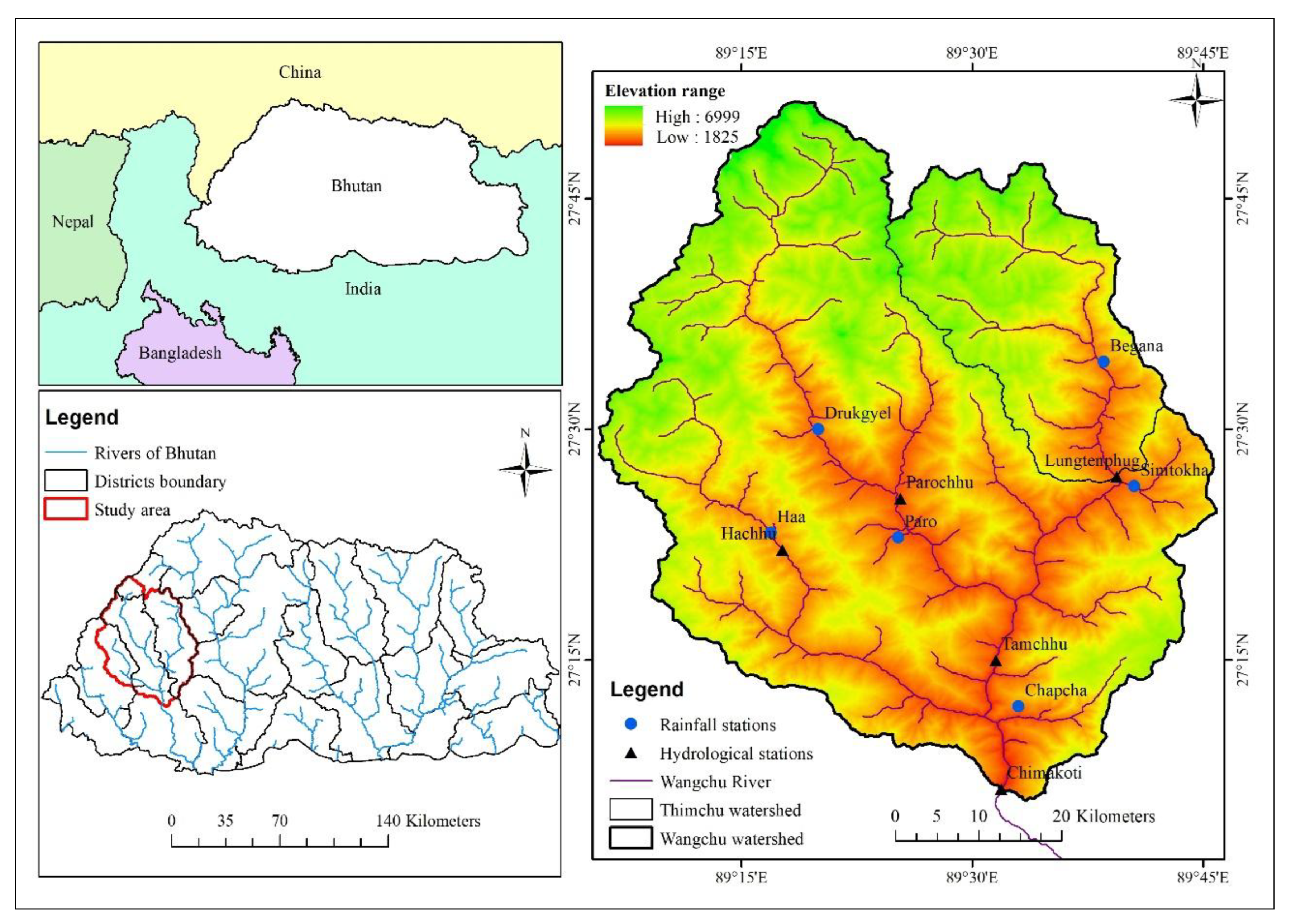
Figure 2.
Schematic research flow.
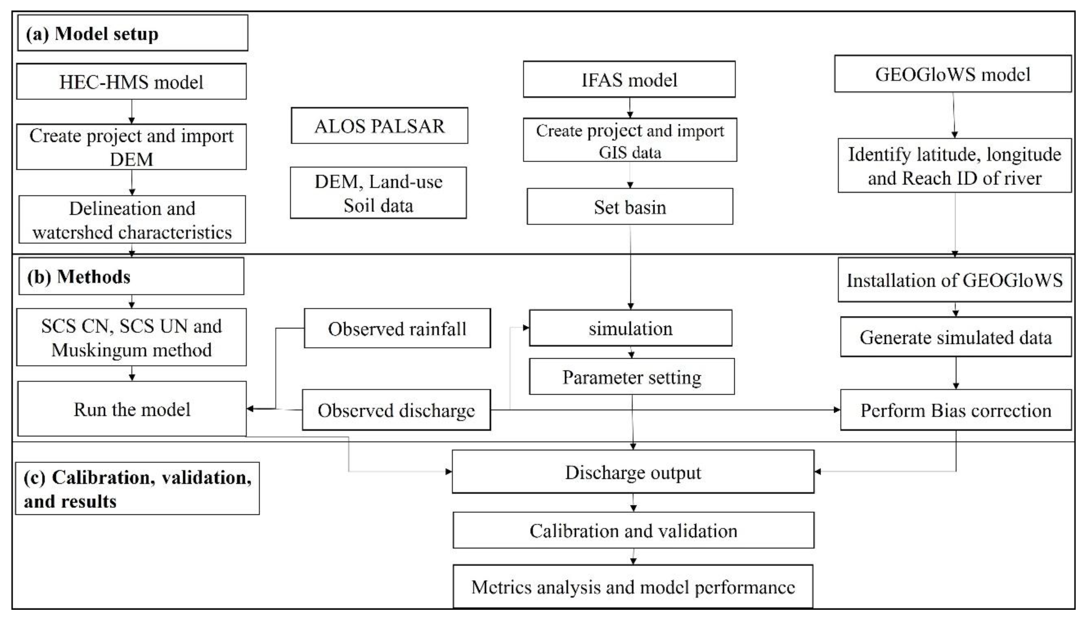
Figure 3.
(a) Subbasins and stream network, (b) curve number, (c) soil classes and (d) land-use classes.
Figure 3.
(a) Subbasins and stream network, (b) curve number, (c) soil classes and (d) land-use classes.
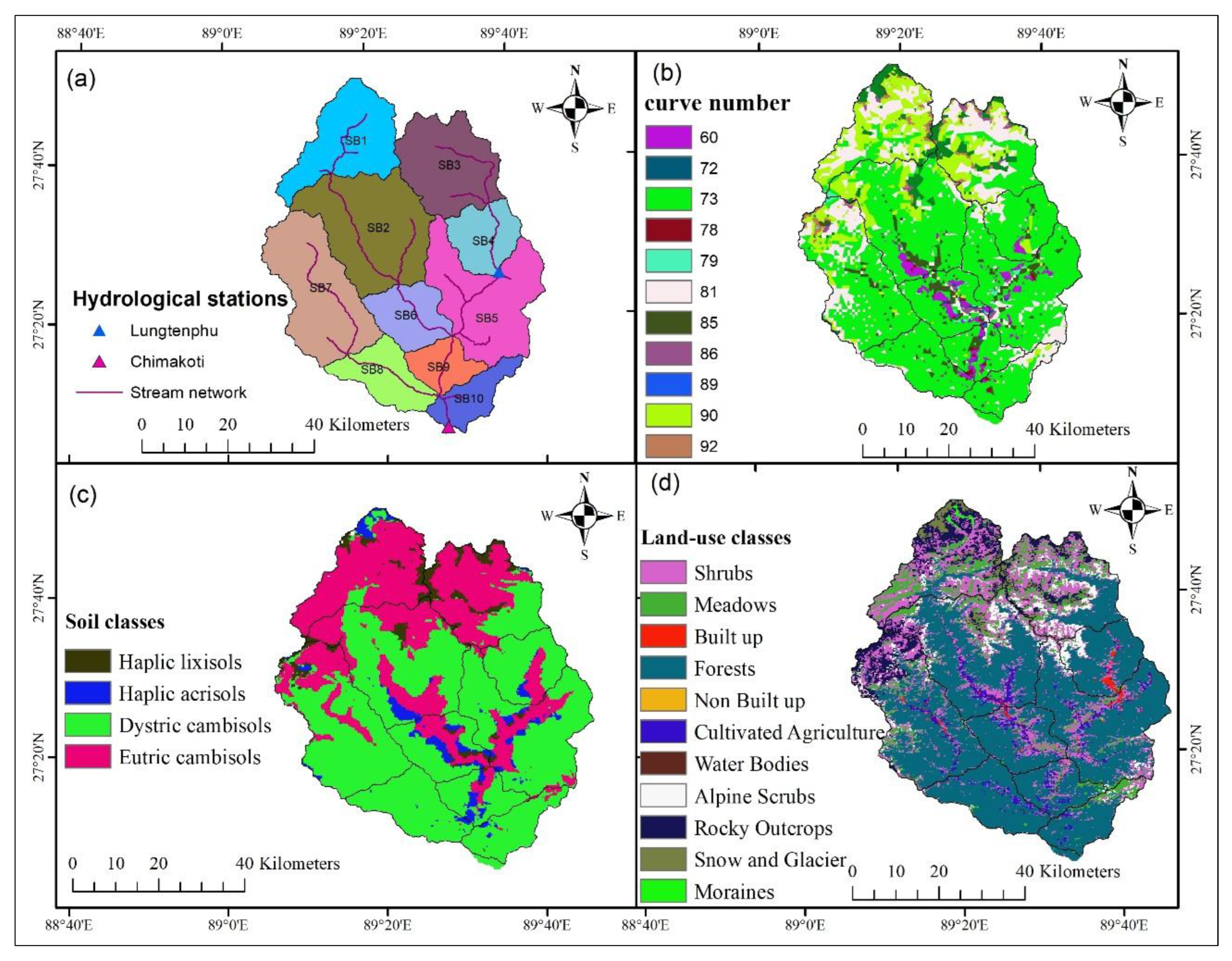
Figure 4.
Validated metrics obtained from the models.
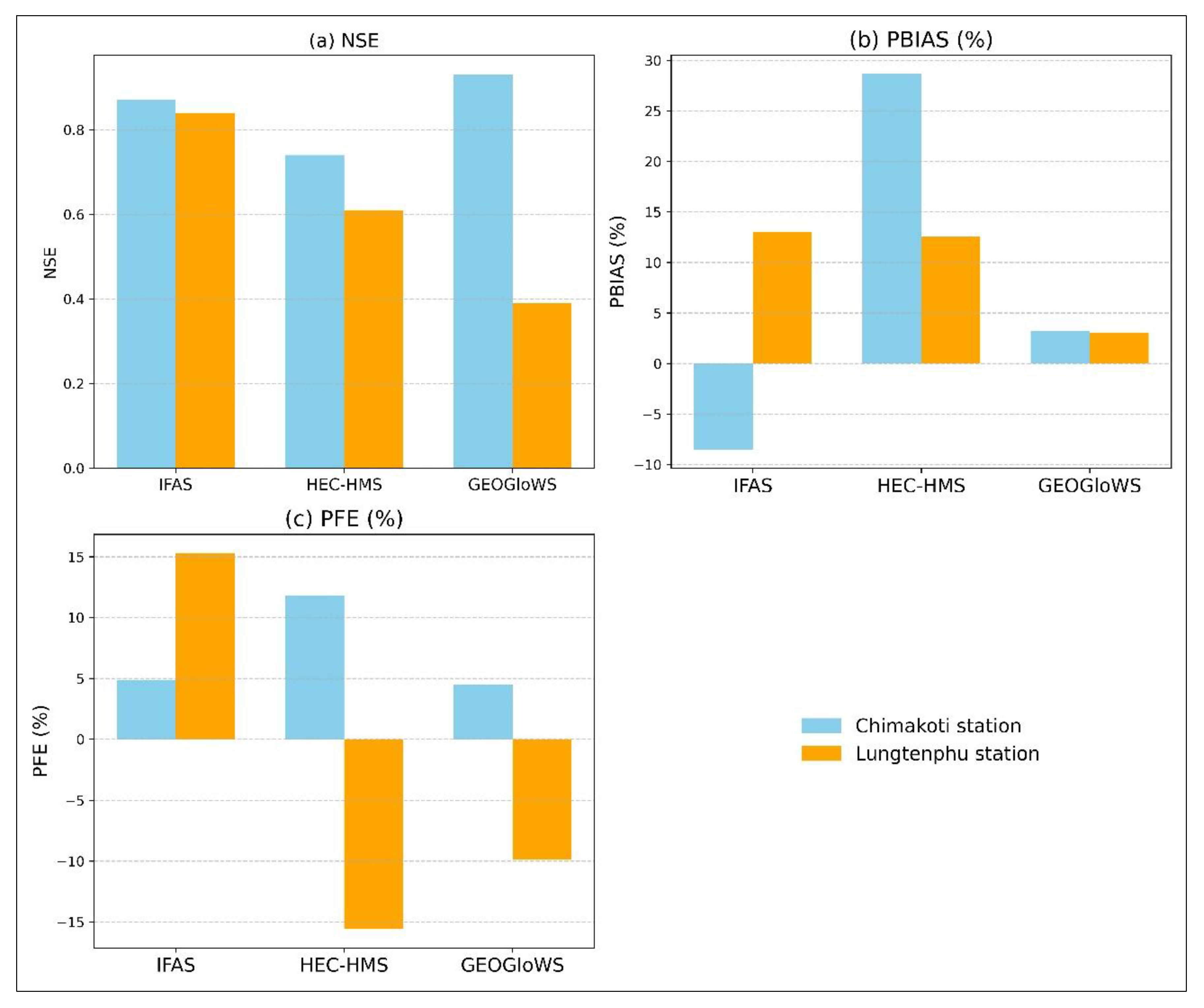
Figure 5.
Calibration and validation using IFAS, HEC-HMS, and GEOGloWS models (a) calibration at Chimakoti (b) validation at Chimakoti (c) calibration at Lungtenphu, and (d) validation at Lungtenphu station.
Figure 5.
Calibration and validation using IFAS, HEC-HMS, and GEOGloWS models (a) calibration at Chimakoti (b) validation at Chimakoti (c) calibration at Lungtenphu, and (d) validation at Lungtenphu station.
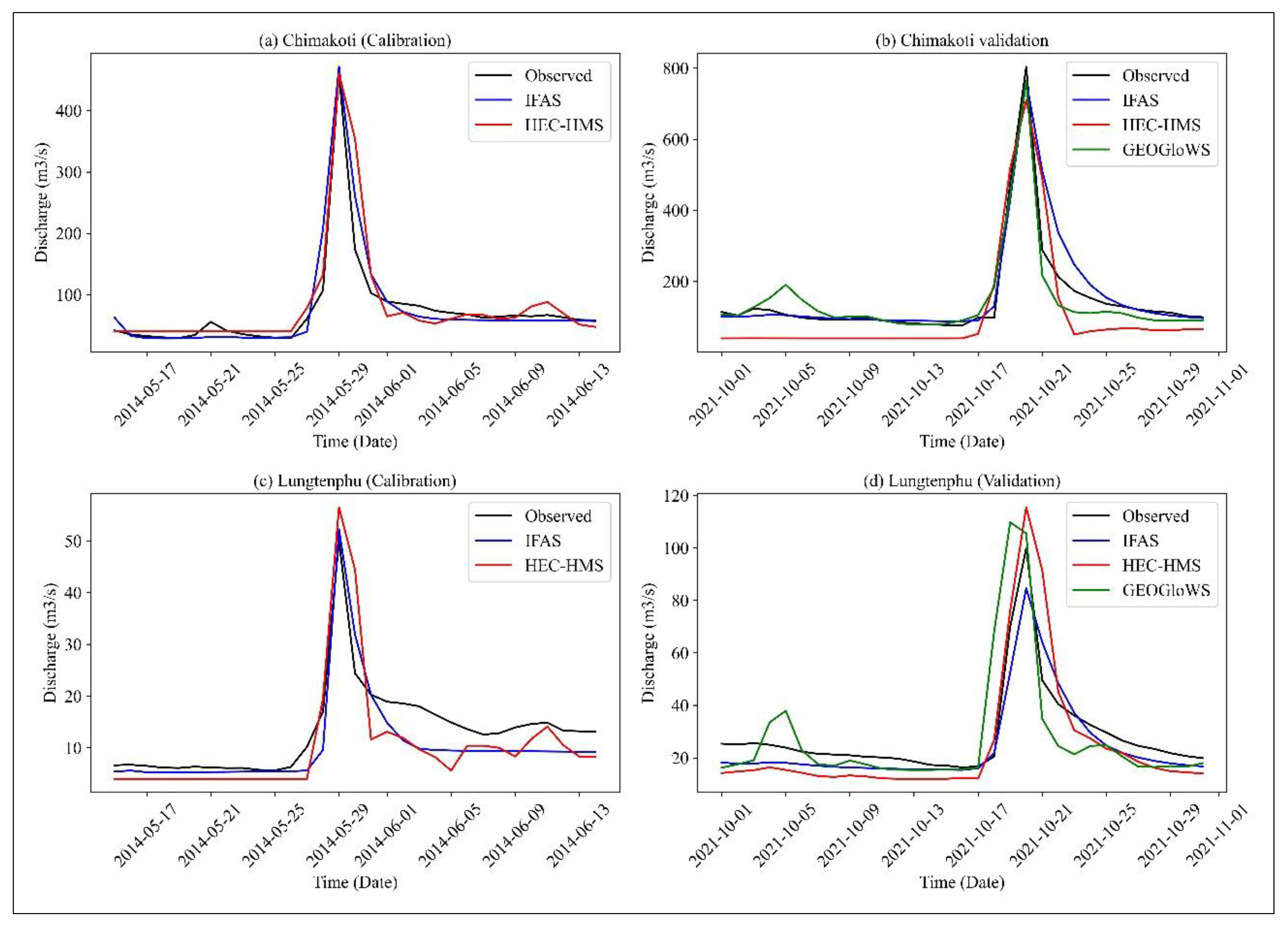

Table 1.
Meteororological and hydrological stations data used in this study.
| Meteorological stations | ||||
|---|---|---|---|---|
| Station Name | Station ID | Latitude | Longitude | Elevation (m) |
| Semtokha | 12700046 | 27.44 | 89.42 | 2504 |
| Begana | - | 27.57 | 89.64 | 2520 |
| Paro | 12510046 | 27.38 | 89.68 | 2402 |
| Drugyel Dzong | 12580046 | 27.50 | 89.33 | 2467 |
| Chapchu | 12390046 | 27.07 | 89.55 | 2620 |
| Haa | 12510046 | 27.39 | 89.28 | 2726 |
| Hydrological stations | ||||
| Lungtenphu | 12800045 | 27.45 | 89.66 | 2260 |
| Chimakoti | 12350073 | 27.11 | 89.53 | 2678 |
Table 2.
Source of satellite data for integrated flood analysis system model.
| Dataset | Elevation | Land-use | Soil |
|---|---|---|---|
| Product name | GTOPO30 | Landuse land-cover | Soil water holding capacity |
| Resolution | 30 arc Second (1km mesh) | 30 arc Second (1km mesh) |
1 degree |
| Format | Raster (Tiles) | Raster (bil) | bil |
| Coordinate | WGS84 | WGS84 | 90ºN and 180ºW |
| Coverage | World | World | World |
| Data source | https://earthexplorer.usgs.gov/ | https://earthexplorer.usgs.gov/ | https://www.fao.org/soils-portal/data-hub/soil-maps |
Table 3.
Calibrated parameters of IFAS model in WRB.
| Tank Model | Parameters | Notations | Units | Default parameter | Calibrated parameters |
|---|---|---|---|---|---|
| Surface tank | Final infiltration capacity | SKF | cm/s | 0.0005 | 0.005 |
| 0.00002 | 0.002 | ||||
| 0.00001 | 0.001 | ||||
| 0.000001 | 0.0001 | ||||
| 0.00001 | 0.0001 | ||||
| Surface roughness coefficient | SNF | m-1/3/s | 0.70 | 1.50 | |
| 2.00 | 2.00 | ||||
| 2.00 | 2.00 | ||||
| 0.10 | 1.00 | ||||
| 2.00 | 2.00 | ||||
| Aquifer tank | Runoff coefficient of unconfined aquifer | AUD | (1/mm/day)1/2 | 0.10 | 0.02 |
| Runoff coefficient of confined aquifer | AGD | 1/day | 0.003 | 0.001 | |
| River course tank | Coefficient for cross section shape | RLCOF | Non-dimensional | 1.4 | 1.4 |
Table 4.
Subbasins characteristic of HEC-HMS model.
| Subbasins | Area (km2) | Length (km) | Centroidal flow path (km) | Slope (degree) | Drainage density (km/km2) |
Curve number |
Lag time (hr) |
|---|---|---|---|---|---|---|---|
| Subbasin1 | 418.32 | 34.75 | 12.23 | 60.03 | 0.066 | 83 | 2.55 |
| Subbasin2 | 617.58 | 48.68 | 19.44 | 57.65 | 0.094 | 78 | 3.54 |
| Subbasin3 | 432.74 | 42.16 | 21.94 | 57.65 | 0.089 | 86 | 3.67 |
| Subbasin4 | 216.68 | 26.90 | 8.97 | 50.48 | 0.093 | 73 | 2.04 |
| Subbasin5 | 533.24 | 39.55 | 15.27 | 50.96 | 0.088 | 65 | 3.84 |
| Subbasin6 | 221.48 | 30.71 | 12.83 | 47.91 | 0.099 | 69 | 2.36 |
| Subbasin7 | 544.14 | 54.01 | 23.51 | 54.39 | 0.084 | 78 | 4.18 |
| Subbasin8 | 227.88 | 34.50 | 14.58 | 52.73 | 0.118 | 60 | 3.16 |
| Subbasin9 | 148.01 | 20.38 | 6.42 | 52.21 | 0.109 | 68 | 2.16 |
| Subbasin10 | 160.38 | 34.41 | 15.29 | 56.99 | 0.088 | 72 | 2.38 |
Table 5.
Calibrated parameters used in HEC-HMS model.
| Parameters | Calibrated values |
|---|---|
|
0.2 |
|
1.9 |
|
7 |
|
0.1 |
Disclaimer/Publisher’s Note: The statements, opinions and data contained in all publications are solely those of the individual author(s) and contributor(s) and not of MDPI and/or the editor(s). MDPI and/or the editor(s) disclaim responsibility for any injury to people or property resulting from any ideas, methods, instructions or products referred to in the content. |
© 2025 by the authors. Licensee MDPI, Basel, Switzerland. This article is an open access article distributed under the terms and conditions of the Creative Commons Attribution (CC BY) license (http://creativecommons.org/licenses/by/4.0/).
Copyright: This open access article is published under a Creative Commons CC BY 4.0 license, which permit the free download, distribution, and reuse, provided that the author and preprint are cited in any reuse.


