
Submitted:
13 November 2024
Posted:
18 November 2024
You are already at the latest version
Abstract
Climate change has a significant impact on river flows, affecting flood risks, especially in Andean regions with complex hydrological dynamics. This study examines flood scenarios in the Cunas River Basin, Junín, Peru, through hydrological and hydraulic simulations under varying climate projections. A multi-model ensemble (MME) approach was employed using CMIP6 climate models. In this analysis, precipitation data were processed, watershed parameters were calculated, peak flows and the extent of floodable areas were estimated. The Hydrologic Engineering Center's Modeling System (HEC-HMS) was employed to simulate peak flows corresponding to return periods of 25, 50, 100, 139 and 200 years, while HEC-RAS was used to map flood zones. Calibration and validation used historical precipitation from nearby stations. The results indicate a consid-erable increase in peak flows and flood prone areas due to climate change. A 6.25% increase in peak flow, a 28.6% expansion in flood-prone areas, and a 37.25% increase in flood depth are observed. These findings highlight the importance of implementing riverbank protection structures. This study provides key insights for flood risk management in the region and highlights the usefulness of advanced modeling tools for understanding the hydrological response to climate change.
Keywords:
climate change
; flood modeling
; hydrological simulation
; Cunas River
; HEC-HMS
; HEC-RAS
; CMIP6 climate scenarios
; multi-model ensemble
1. Introduction
Floods are considered among the most frequent and devastating natural disasters globally [1]. These events, often associated with intense and brief rainfall events, have been classified as severe and economically destructive disasters [2]. In recent decades, both the magnitude and frequency of floods have increased markedly worldwide [3,4]. This increase is largely related to climate change, which intensifies and increases the frequency of extreme weather events [5].
Climate change has a significant impact on the probability and intensity of these extreme events, including intense precipitation [6]. In addition, it affects the flow of rivers, causing major alterations in global hydrological regimes [7,8,9]. Extreme meteorological precipitation is especially problematic due to its unpredictable and destructive nature and can cause flash floods and severe floods that overload infrastructure and cause significant material damage [10,11]. Approximately 47% of climate disasters are caused by flooding [12]. To address these risks, it is crucial to have a complete understanding of the factors related to climate change and its impact on the hydrological cycle [13].
It is important to take into account Global Climate Models (GCMs) to have a better understanding of the climate system and the different past and future alterations it presents [14], through the global climate modeling framework of the Coupled Model In- tercomparison Project (CMIP), now called (CMIP6), established as the latest version of the sixth assessment report (AR6) of the Intergovernmental Panel on Climate Change (IPCC) [15,16].
Mathematical modeling and runoff simulation have become fundamental tools in modern hydrologic research and engineering [17,18]. Programs such as the HEC-HMS, developed by the U.S. Army Corps of Engineers, have become a USA, they are widely used to simulate hydrological processes in watersheds with various characteristics [19]. These models make it possible to evaluate how watersheds respond to extreme precipitation and how changes in land use in the upper zones affect flooding patterns in the lower areas [20,21,22].
The threat of devastating floods continues to be a significant global hazard [23]. Human activities and climate change have altered the hydrological cycle, adversely affecting river ecosystems [24,25]. Hydrological simulation and runoff prediction have become increasingly relevant for risk management and disaster mitigation [26,27,28]. HEC-HMS, in particular has been highlighted as a crucial tool in this context, being one of the most widely used tools for simulating rainfall-runoff and analyzing hydrological response in both urban and natural watersheds [29,30].
The relationship between flood discharge probabilities and extreme precipitation is not yet fully explored in the literature, which poses an area of great theoretical and practical interest [31]. Medium- and long-term runoff prediction is crucial to better understand how watersheds react to extreme events and to develop effective risk management strategies [32,33,34]. It is estimated that, by the end of this century, global surface temperatures will rise between 1.4 and 5.8 °C, which will increase the frequency and severity of extreme weather events in various parts of the planet [35]. The natural water cycle in river basins is being put at risk by climate change, which intensifies the importance of these studies [36,37]. In some regions of South America, water use and deforestation have amplified the effects of climate change on extreme flow rates, causing more severe droughts and more intense floods [38]. In the city of Huancayo (Peru), this risk is present due to the increase in the flow of the Cunas River during periods of heavy rainfall, according to reports from the Instituto Nacional de Defensa civil. These rains cause floods that represent a significant risk, endangering homes, fish farms and agricultural crops, generating potentially catastrophic damage and threatening the safety of the community in the district of Pilcomayo, in the Junín region (Peru) [39]. Earlier this year, it was estimated that 12 houses collapsed, property was damaged, and livelihoods (agriculture and fish farms) were affected, generating estimated losses of approximately US$ 135,000 [39]. Floods not only negatively impact social and economic conditions, generating high levels of unemployment and worsening public health, but also damage the ecosystem [40,41].
The main objective of this research is to evaluate the behavior of the Cunas River, estimate the maximum design flow for different return periods (T = 50, 100, 139 and 200 years) under normal conditions and climate change scenarios, and identify the maximum floodable areas for these scenarios. As demonstrated for precipitation, the climate change scenarios project that the maximum 24-hour precipitation increases significantly compared to current conditions. In addition, the return period of 20-year events would be shortened to about 14 years, indicating a higher frequency of extreme events [42]. For the evaluation and prediction of climate change, 10 CMIP6 global climate models (GCMs) were used, which were part of the last IPCC report [16], adjusted for the region by means of bias correction and statistical reduction, referenced with local data, including the RAIN4PE product for precipitation and PISCO for temperatures. Historical information was collected from the San Juan de Jarpa and Huayao pluviometric stations, corresponding to the period 1974- 2023. This information was used to calculate the design flow in both scenarios using HEC-HMS software. Subsequently, a simulation of the water flow in the study area was carried out using the HEC-RAS software, in order to identify and compare the risk areas in the event of a possible flood, for normal conditions, as well as in a scenario under the influence of climate change.
2. Data and Methodology
The methodological flow followed in this study is summarized in (Figure 1). The topographic data, obtained from the DEM (5x5 m resolution), were processed in QGIS (v. 3.34.5), while the precipitation data were obtained from ANA-SENAMHI and the CMIP6 climate models. Subsequently, the data were subjected to quality control and processing before being integrated into the HEC-HMS model software (v. 4.12), using the curve number (CN) method to simulate peak flows for different return periods. The results of the hydrological modeling were fed into the HEC-RAS model (v. 6.5), performing the hydraulic simulations and identifying the flood-prone areas with RAS-Mapper, which allowed a comprehensive evaluation of the flood risk in the Cunas River basin.
2.1. Study Area
The Cunas River basin is located in the department of Junín, originating in the Western Cordillera at 4953 masl, it crosses the provinces of Chupaca, Concepción and Huancayo and flows into the Mantaro River at approximately 3216 masl. It has a surface area of 1700.25 km²/s and a length of 93,79 km. The Cunas River is an important tributary of the Mantaro River, which in turn is part of the Amazon basin [43].
To obtain topographic information and to integrate the topographic data obtained from the digital elevation models (DEM) with a spatial resolution of 5 meters, the QGIS software version (3.34.5) was used. The drainage network (main and tributary streams), the basin boundaries (precise delimitation of the basin) and the alti- metry (Figure 2) were delineated, calculating the morphometric properties of the basin (Table 1).
2.2. Area of the Micro-Watersed
The microbasin of analysis and the area of this study is located northeast of the study basin. It has an area of 186.07 km²/s , a channel length of 33.31 km, and a slope of 1%. The pluviometric stations used in this study are located in the district of San Juan de Jarpa and the town of Huayao (Figure 3).
2.3. Hydrological Study under Normal Conditions
2.3.1. Influence and Analysis of Precipitation
Precipitation was estimated using the Huayao and San Juan de Jarpa rainfall stations. This information was provided by the Servicio Nacional de Meteorología e Hidrología del Perú (SENAMHI), and the Autoridad Nacional del Agua (ANA), 50 daily rainfall data from 1974 to 2023 were considered.
The Thiessen polygon method was used to distribute the maximum and average rainfall in a basin in an equitable manner, which, by means of perpendicular lines between each pair of adjacent stations, form polygons that represent the areas of influence of each station [44]. The area of the Huayao station is 108.02 km²/s y San Juan de Jarpa is 77.45 km²/s, likewise the coefficients obtained through Equation (1) were 0.41623 and 0.58377 respectively.
Where, is the weighted or average precipitation in the basin (in mm), is the area of the polygon corresponding to station (in Km²/s), is the total area (en Km²/s), is the precipitation measured at the station (in mm) y is the total number of stations. According to the statistical analysis of doubtful data with a significance level of 10 % for a normal distribution, the range of precipitation is between a minimum of 17.86 mm and an acceptable maximum of 48.27 mm.
Using the Kolmogorov-Smirnov goodness-of-fit tests, it was determined that the best fit for calculating the maximum annual precipitation for the return periods of 2,5,10,25,50,100,139,200 and 500 years is that of Pearson III with 99.63%. In addition, a correction was made for the fixed interval factor of 1.13 applied to the maximum annual precipitation [45].
The present investigation was carried out for a return period of 139 years to determine flood-prone areas, as established in the Manual of the Peruvian Ministry of Transport and Communications (MTC) for the design of river defense works. This return period is important to ensure that a structure of this type, projected for the future, is capable of mitigating floods based on an extreme event with a specific probability of occurrence. [46].
Subsequently, the IDF curves were calculated using the Dyck-Peschky model, and through a multiple regression analysis, the intensity was obtained for the aforementioned return periods, which allowed the elaboration of the hyetograph using the alternating block method, used to analyze the temporal distribution of rainfall in different return periods [47]. The hyetograph shows the rainfall intensity in specific time intervals every 1 hour, providing crucial information for hydrological modeling. The design rainfall hyetograph for a 139-year return period is shown below (Figure 4).
2.3.2. Estimation of Maximum Flow rate (Qmáx) in HEC-HMS
Initially, the HEC-HMS program version 4.12 was used to estimate the maximum flow under normal conditions for different return periods. The SCS Curve Number (CN) method was used to estimate the direct runoff from precipitation. [48]. Curve numbers were determined as a function of land use, soil type, and moisture conditions. The CN values range from 0 to 100, where higher values indicate higher runoff and lower infiltration. For the calculation of the Curve Number (CN) in the sub-basin, we used data in wet conditions downloaded from the shapefile prepared by the ANA. This shapefile was processed in QGIS to delimit the specific area of our sub-basin. Equation (2) helped us to calculate the CN, giving a total of 91.85 curves, being an important data to consider.
The time of concentration (Tc) is a fundamental concept in hydrology that measures the response of a watershed to a rainfall event and is defined as the time required for all areas of the watershed to contribute to runoff at its outflow point [49]. This parameter is essential for evaluating the hydrologic response of the watershed and for estimating maximum flows in hydrologic design [49]. The different methods established to calculate Tc were compared, highlighting those whose variability within the acceptable range is considered valid. The average Tc values calculated for the hydrographic unit studied is 7.08 hours (Table 2).
With a calculated time of concentration (Tc), the delay time (Tp) was determined by applying a coefficient of 0.6, which resulted in 4.25 hours.
2.3.3. Simulación del Comportamiento del rio Cunas con HEC-RAS
The behavior of the Cunas River was simulated using HEC-RAS ver. 6.5 to predict flooding, to evaluate the initial scenario and the current scenario in the presence of climate change. The Cunas River was imported in Shape format.
The channel line was drawn following the axis of the natural channel and was used to define the cross sections. Bank Lines delineate the main channel, and Flow Paths in the floodplain define the limits of the overflows. Cross Sections were drawn perpendicular to the water flow and extended outside the flow line boundaries. Seventeen cross sections were created, 150 meters wide and spaced every 100 meters apart (Figure 5). For the calculations in HEC-RAS, flow data were entered with peak flows calculated for a return period of 139 years. The Manning's coefficient of 0.032 and the downstream slope were also entered, with a value of 0.01.
After defining the geometry, the data were imported into HEC-RAS, where errors were corrected with the Cross Section Point Filter tool. Flood simulation was performed to evaluate the magnitude and impact of floods in the study area, using HEC-RAS software for modeling flows in rivers and channels [50]. HEC-RAS, developed by the U.S. Army Corps of Engineers, uses mass and momentum conservation equations to analyze flows and assess flood risks [19].
The methodology used combines HEC-RAS and ArcGIS to assess flood risk, using topographic maps and digital terrain models. Cross-sectional profiles were created in ArcGIS and imported into HEC-RAS for calibration and analysis. The modeling allows assessment of the extent of flooding and calculation of potential damage.
2.4. Hydrological Study with the Presence of Climate Change
2.4.1. Influence and Analysis of Precipitation
Climate data simulated by CMIP6 Global Climate Models (GCMs) were analyzed using the VECC (Visualización de Escenarios Climáticos y Capacidades) tool of the Mantaro Basin Observatory (https://observatoriomantaro.ana.gob.pe/es-es), adjusted specifically for the region and the study area. The analysis focused on annual maximum daily precipitation, based on 10 global climate models (CanESM5, CNRM-CM6-1, CNRM-ESM²/S-1, GFDL-ESM4, IPSL-CM6A-LR, MIROC6, MPI-ESM1-2-HR, MRI-ESM²/S-0 y UKESM1-0-LL). Each model has its own SSP scenarios; these scenarios were developed to investigate global development trajectories with respect to climate change. They assess the impact of socioeconomic trends and policies on greenhouse gas emissions, climate change and social resilience [51]. This research opted for the SSP5-8.5 shared socioeconomic trajectory scenario that projects an additional radiative forcing of 8.5 W/m² by the year 2100, which could increase global temperature by 2.42 to 5.64 °C, with significant impacts on flood risk [52].
The Multi-Model Ensemble (MME) approach was employed to analyze annual maximum daily precipitation using 10 global climate models over the period 1981-2023. This approach, widely used in previous studies [53,54,55], improves the accuracy of climate projections by integrating the results of different models. CMIP6 models, under the SSP5-8.5 climate scenario. The process consists of averaging the precipitation values for each year and model, thus generating an MME that represents the average annual maximum daily precipitation for the unified micro basin (Figure 6). Based on this time series that reflects the effects of climate change, a correction factor is calculated and applied to the maximum annual precipitation for the estimated return times, thus adjusting the estimates to the new projected climate conditions.
Based on this time series reflecting the MME approach, a correction for the influence of climate change was made with a factor of 1.18 derived from the analysis of both precipitation data (historical and MME), thus adjusting the estimates to the new projected climate conditions. The factor was applied to the maximum annual precipitation for the different return years under a Pearson III adjustment obtained from the Kolmogorov-Smirnov goodness-of-fit tests. With the estimation of these new precipitations, the new IDF curves were calculated using the Dyck-Peschky model, and as had been done previously, the intensity for the return periods under study was obtained through the same multiple regression analysis. Subsequently, the design rainfall hyetograph was prepared for the different return periods, highlighting the return period of 139 years, at specific time intervals of 1 hour (Figure 7).
2.4.2. Maximum Flow Rate Estimation (Qmáx ) in HEC-HMS and Simulation with HEC-RAS
The estimation of the maximum flow rate will be determined in the same way that the flow rates were estimated under normal conditions. The time of concentration (Tc) calculated above is 7.08 hours and the delay time (Tp) is 4.25 hours. These values were worked out the same in both conditions, because the formulas used for the calculation are independent of rainfall and depend on the morphological characteristics of t h e study basin, which is the same for both scenarios being worked on.
Similarly, HEC-RAS was used for the simulation to evaluate flooding under the influence of climate change.
3. Results
3.1. Calculation of Maximum Design Flow and Volumes Using HEC-HMS
After carrying out the hydrological analysis of the Cunas River through the HECHMS program, the maximum flows and volumes in the analysis area (precipitation, losses, excess and discharge) were obtained for the two situations analyzed (normal conditions and with the presence of climate change) and for the return periods of 25, 50, 100, 139 and 200 years, whose main analysis result was focused on the 139-year return period, due to the focus of the study.
Table 3 shows that the maximum flow for a 139-year return period under normal conditions was 183.10 m³/s, while with the presence of climate change it was 195.30 m³/s , which indicates that, due to the influence of climate change, the flow increased by 6.25% compared to normal conditions. Similarly, the volume of direct runoff or discharge for a return period of 139 years under normal conditions was 28.61 mm and with the presence of climate change it was 30.49 mm, which indicates an increase in volume. 6.17% when including the presence of climate change. These increases, both in volume and maximum flows, highlight the growing influence of the climate scenarios applied to our analysis, which highlights the importance of considering climate change as an important variable in the planning of preventive measures against possible hydrological risks such as floods.
In addition, Table 3 shows that there is an increase in volumes and flows as the return periods are longer, because as the return period is longer, the frequency of occurrence is lower, but with greater intensity, and when climate change is included, these values will have a much more significant increase.
On the other hand, for a better management and scope of the results obtained, the hydrographs (flow-time) were obtained, which by means of a graphic representation shows the variation of the flow of the Cunas River as a function of the time given in minutes, in response to the previously analyzed rainfall. These hydrographs were the result of the analyses performed in HEC-HMS, which, after data processing, the program gave us these graphs independently for each return period and in hours. Subsequently, after adjusting the information, the hydrographs shown in Figure 8 were obtained for the return periods of 25, 50, 100, 139 and 200 years under normal conditions (Figure 8a) and with the presence of climate change (Figure 8b), whose color variation refers to each return period. Although it is true that these hydrographs appear together with the flow rates obtained in Table 3, the importance of these graphs is based on a better understanding of the hydraulic process as a function of time, since it can be seen in both graphs that the flow rate first rises until it reaches the maximum peak (maximum flow rate) and then undergoes a gradual increase in water flow, resembling the shape of a bell. In addition, the duration of the runoff event in the basin is identified, which is very useful for the management of water resources and the design of hydraulic works.
Figure 8 shows the hydrographs between flow rate (m³/s) and time in 30-minute intervals for the two conditions worked and for the return periods established above.
Figure 8a shows the hydrograph under normal conditions, whose maximum peak for the 139-year return period is 183.10 m³/s, reaching its maximum value at 1020 minutes (17:00 hours). On the other hand, Figure 8b shows the hydrograph with the presence of climate change, whose temporal distributions of the flow show higher peaks compared to normal conditions. For the 139-year return period, the maximum peak is 195.30 m³/s , also at 1020 minutes (17:00), increasing its value by 6.25%.
This indicates that, for both cases, in that period of time, the water has accumulated enough to generate the highest flow of the event that occurred in this particular hour, and the time of concentration found above is part of this result.
3.2. Flood Simulation (flooded Areas and Sections)
With the hydrological data obtained previously and using the HEC-RAS program, we simulated the flood areas and zones of the Cunas River for a return period of 139 years (Figure 9), under normal conditions (Figure 9a) and with the influence of climate change (Figure 9b).
Figure 9a shows the flood model made under normal conditions, whose floodable area was 159,111.38 m²/s . The main area affected would be the La Perla Shopping Center, where it was estimated that 30 houses bordering the Cunas River would be directly affected, most of which are located on Eternidad Road; 38% of the surface area of the Chupaca General Cemetery located on Eternidad Road would also be affected. Likewise, 38 agricultural lands located on both banks of the river, dedicated to crop production (potato, corn, barley, wheat, quinoa) and livestock raising (cows, pigs, sheep, chickens, hens) would be affected, with a total area of approximately 33,459 m²/s , representing 21% of the total flooded area. The main road that gives direct access to the province of Chupaca, called Eternidad, was also affected to a lesser extent.
Figure 9b shows the flooding model carried out with the influence of climate change, whose flooding area amounted to 222,823.67 m²/s , which would directly affect 120 houses in La Perla, located on Raymondi, Los Angeles and Eternidad streets. The Chupaca General Cemetery would be affected by 52% of its surface area and recreational and tourist areas would also be affected. Also affected would be 45 agricultural fields, located on both banks of the river, dedicated to crop production and livestock raising, with a total area of approximately 56,574 m²/s , representing 25.39% of the total flooded area. Urban areas such as Raymondi and Los Angeles and the main road Eternidad, which gives direct access to the province of Chupaca, would also be significantly affected.
The increase in flooded area under the effects of climate change represents 28.6% compared to normal conditions, which is mainly reflected in peripheral areas of La Perla, where the flat topography favors the extension of water flow. For both events, it is shown that the flood depth has a maximum of 5.123 m in critical areas and varies according to the intensity of colors shown in both cases. When comparing both events, there is a significant variation in the extent of flooded areas, while on the one hand, when simulating under normal conditions, there are less vulnerable flooded areas with a moderate impact on urban areas, on the other hand, when including the effect of climate change, a considerable increase in flooded areas is observed, also affecting main roads such as the one that gives access to the province of Chupaca, with more severe future projections. These projections would involve flooding affecting many more homes in La Perla and a main road called Coronel Parra, located at the other end of the Cunas River, with access to the province of Chupaca and the districts of Huáchac.
The simulation performed with HEC-RAS also allowed us to visualize the cross sections along the entire length of the Cunas River, which helped us to know in detail the geometry of the river and the heights of each established section, and also allowed us to know the behavior of the water flow in the different widths and depths of the river.
Figure 10 shows mainly the most critical sections of the Cunas River analysis section, for a return period of 139 years and under the two conditions studied: for normal conditions (Figure 10a) and with the influence of climate change (Figure 10b). In both cases it is observed that the river in this section reveals the shape of a U, whose right lateral margin has a much higher level compared to the left lateral margin, due to the topography of the Cunas River.
Figure 10a shows that the cross section under normal conditions has a height of 8.70 m, which, when simulating the flood, the water level rose to a height of 3.2 m above the river level.
In Figure 10b worked with the influence of climate change, it can be seen that the elevation height was 10.60 m and the flood height increased to 5.1 meters.
The increase in altitude with the presence of climate change is significantly 1.9 m compared to normal conditions, increasing by 37.25%.
Likewise, this simulation reflects the capacity that the flood generates over the years, by having turbulent flows of mass removal and laminar flows with a great potential to wear away the materials accumulated on the edges of the channel and accumulate sediments on the bottom of the river along its path, causing the margins of the river channel to progressively extend over time, and added to this, by not having prevention and mitigation measures such as the construction of riverside defense structures (dams, gabions, retaining walls, etc.) they allow the surrounding population to be more vulnerable to these events.
4. Discussion
For the study carried out, after the hydrological analysis performed under the CMIP6 models, the results obtained were the maximum flows under normal conditions and with the influence of climate change, showing an increase of 6.25% of flow when including climate change, which, this increase depends on many factors such as the place where the study is carried out, for the case of the study carried out in the Anya River, the increase in flows through the RCP 8.5 scenario would amount to 12.6% by the year 2100 [56].
another study would indicate that the annual flow of the Lurin river, estimated in a medium zone and using the same scenario, would increase from 14 to 44% [57], while in more distant places such as Ireland, the increase obtained for the decade of 2080 would be 13.09%, also working with the RCP 8.5 scenario [58].
The influence of climate change on flood levels affects river flows [58], which translates into a greater risk for nearby communities and ecosystems, which may not be prepared to face this type of scenario.
The simulations carried out under normal conditions and scenarios with the presence of climate change clearly show how the flood areas expand when the maximum flows increase [59], increasing by 28.6%, which, when the flood simulations are carried out, both housing and agricultural land would be the most vulnerable, but the greatest impact would be generated in agricultural areas, resulting in 21% for normal conditions and 25.29% with the presence of climate change; in other cases, it was estimated that the cultivated areas would account for approximately 90% of the total flood area [60], due to the fact that agricultural lands are located outside urban areas because of the large extensions they require and for the use of water, which represents 70% of water withdrawals [61], since agriculture is considered fundamental due to the constant pressure exerted by population growth and total food consumption [62].
As has been shown, the extent of flooded areas exceeds river levels [63], reaching heights of approximately 3.2 m under normal conditions and increasing by 1.9 m with the presence of climate change, reaching a total height of 5.1 m. This increase has critical implications, since it causes the river to exceed its natural limits in previously unaffected sectors, which significantly increases the flooded area and its severity. This increase has critical implications, since it causes the river to exceed its natural limits in previously unaffected sectors, which significantly increases the flooded area and its severity. From a risk management perspective, these increases in flood depth require comprehensive planning that considers both the adaptation of existing infrastructure and the implementation of early warning systems and flood mitigation strategies in the same manner as mentioned in [64]. Given that climate change will continue to alter precipitation and flow patterns, it is imperative to conduct periodic assessments and adjust risk models based on new projections.
In particular, the critical section area requires priority attention in future interventions, as its geographic characteristics and current vulnerability could be disastrous under future climate scenarios. This study reaffirms these findings by showing that the shorter return periods already reflect higher flows than those estimated under normal conditions. This phenomenon increases the frequency of severe hydrological events, coinciding with the observations of [65], who note that flood events that were previously considered improbable in short periods of time are now more likely to occur.
These findings corroborate that even minor increases in flow can translate into much greater impacts on river carrying capacity and water distribution in surrounding areas. Climate change has been shown to alter hydrological patterns, intensifying extreme events such as heavy rainfall and, consequently, peak river flows [66].
The importance of these findings lies in their direct implication for the planning of risk management and climate change adaptation measures. The fact that the simulations show more extensive overflows under climate scenarios highlights the need to incorporate such scenarios into disaster mitigation plans. As pointed out by [67], climate change requires a reconfiguration of risk management strategies, which must include more dynamic and flexible planning in the face of changing environmental conditions. For this reason, it is possible to propose directions of research such as socioeconomic analysis of the impact of floods or adaptation and mitigation of green infrastructure.
5. Conclusion
When performing the hydrological and hydraulic analysis under normal conditions, minimal variations were observed in the study area (Cunas River); however, when climate change was included, the results increased considerably and the use of the 10 Global Climate Models (GCMs) of the CMIP6 were of great importance to determine this variation.
After the analysis carried out for normal conditions and conditions with the presence of climate change, the maximum flow for normal conditions was of 183.10 m³/s, while with the presence of climate change the maximum flow was of 195.30 m³/s, generating an estimated increase of 6.25%.
When the simulation was carried out under normal conditions, a floodable area of 159,111.38 m² was obtained, while in the presence of climate change, an area of 222,823.67 m² was obtained.
This study emphasizes that climate variability and the increase in projected flows produce significant increases in the severity and extent of flooding with the presence of climate change, with a 28.6% increase over flooding under normal conditions, which would affect the population, homes, agricultural areas, schools, tourist recreation areas and streets, mainly in the La Perla population center.
Under normal conditions it was determined that 30 houses and approximately 38 agricultural lands with total areas of 33,459 m²/s dedicated to crop production and livestock raising would be affected, while with the influence of climate change 120 houses directly and 45 agricultural lands with a total area of 56,574 m²/s would be affected.
The simulation using the HEC RAS obtained flood heights of 3.2 m for normal conditions and 5.1 m with the presence of climate change, resulting in an increase of 37.25%.
The research highlights the urgent need to include climate change scenarios in risk management plans, underscoring the importance of more flexible and dynamic strategies to mitigate the impact of disasters. The integration of these findings into urban and rural development plans will be essential to protect affected communities, minimizing both the risk of material damage and potential economic losses in the presence of future extreme events.
References
- Samarasinghe, J.T.; Makumbura, R.K.; Wickramarachchi, C.; Sirisena, J.; Gunathilake, M.B.; Muttil, N.; Teo, F.Y.; Rathnayake, U. The Assessment of Climate Change Impacts and Land-use Changes on Flood Characteristics: The Case Study of the Kelani River Basin, Sri Lanka. Hydrology 2022, 9, 177. [Google Scholar] [CrossRef]
- Nguyen, H.Q.; Degener, J.; Kappas, M. Flash Flood Prediction by Coupling KINEROS2 and HEC-RAS Models for Tropical Regions of Northern Vietnam. Hydrology 2015, 2, 242–265. [Google Scholar] [CrossRef]
- Bhusal, A.; Parajuli, U.; Regmi, S.; Kalra, A. Application of Machine Learning and Process-Based Models for Rainfall-Runoff Simulation in DuPage River Basin, Illinois. Hydrology 2022, 9, 117. [Google Scholar] [CrossRef]
- Nabinejad, S.; Schüttrumpf, H. Agent-Based Modeling for Household Decision-Making in Adoption of Private Flood Mitigation Measures: The Upper Kan Catchment Case Study. Water 2024, 16, 2027. [Google Scholar] [CrossRef]
- Dhanapala, L.; Gunarathna, M.H.J.P.; Kumari, M.K.N.; Ranagalage, M.; Sakai, K.; Meegastenna, T.J. Towards Coupling of 1D and 2D Models for Flood Simulation—A Case Study of Nilwala River Basin, Sri Lanka. Hydrology 2022, 9, 17. [Google Scholar] [CrossRef]
- Quintero, F.; Mantilla, R.; Anderson, C.; Claman, D.; Krajewski, W. Assessment of Changes in Flood Frequency Due to the Effects of Climate Change: Implications for Engineering Design. Hydrology 2018, 5, 19. [Google Scholar] [CrossRef]
- Iliadis, C.; Galiatsatou, P.; Glenis, V.; Prinos, P.; Kilsby, C. Urban Flood Modelling under Extreme Rainfall Conditions for Building-Level Flood Exposure Analysis. Hydrology 2023, 10, 172. [Google Scholar] [CrossRef]
- Gruss, Ł.; Wiatkowski, M.; Połomski, M.; Szewczyk, Ł.; Tomczyk, P. Analysis of Changes in Water Flow after Passing through the Planned Dam Reservoir Using a Mixture Distribution in the Face of Climate Change: A Case Study of the Nysa Kłodzka River, Poland. Hydrology 2023, 10, 226. [Google Scholar] [CrossRef]
- Souley Tangam, I.; Yonaba, R.; Niang, D.; Adamou, M.M.; Keïta, A.; Karambiri, H. Daily Simulation of the Rainfall–Runoff Relationship in the Sirba River Basin in West Africa: Insights from the HEC-HMS Model. Hydrology 2024, 11, 34. [Google Scholar] [CrossRef]
- Huo, L.; Sha, J.; Wang, B.; Li, G.; Ma, Q.; Ding, Y. Revelation and Projection of Historic and Future Precipitation Characteristics in the Haihe River Basin, China. Water 2023, 15, 3245. [Google Scholar] [CrossRef]
- Pabasara, K.; Gunawardhana, L.; Bamunawala, J.; Sirisena, J.; Rajapakse, L. Significance of Multi-Variable Model Calibration in Hydrological Simulations within Data-Scarce River Basins: A Case Study in the Dry-Zone of Sri Lanka. Hydrology 2024, 11, 116. [Google Scholar] [CrossRef]
- Shuaibu, A.; Hounkpè, J.; Bossa, Y.A.; Kalin, R.M. Flood Risk Assessment and Mapping in the Hadejia River Basin, Nigeria, Using Hydro-Geomorphic Approach and Multi-Criterion Decision-Making Method. Water 2022, 14, 3709. [Google Scholar] [CrossRef]
- Wang, X.; Xia, X.; Teng, R.; Gu, X.; Zhang, Q. Risk Assessment of Dike Based on Risk Chain Model and Fuzzy Influence Diagram. Water 2023, 15, 108. [Google Scholar] [CrossRef]
- Babaousmail, H.; Ayugi, B.O.; Lim Kam Sian, K.T.C.; Randriatsara, H.H.-R.H.; Mumo, R. How Do CMIP6 HighResMIP Models Perform in Simulating Precipitation Extremes over East Africa? Hydrology 2024, 11, 106. [Google Scholar] [CrossRef]
- Colín-García, G.; Palacios-Vélez, E.; López-Pérez, A.; Bolaños-González, M.A.; Flores-Magdaleno, H.; Ascencio-Hernández, R.; Canales-Islas, E.I. Evaluation of the Impact of Climate Change on the Water Balance of the Mixteco River Basin with the SWAT Model. Hydrology 2024, 11, 45. [Google Scholar] [CrossRef]
- Golian, S.; El-Idrysy, H.; Stambuk, D. Using CMIP6 Models to Assess Future Climate Change Effects on Mine Sites in Kazakhstan. Hydrology 2023, 10, 150. [Google Scholar] [CrossRef]
- Bruno, L.S.; Mattos, T.S.; Oliveira, P.T.S.; Almagro, A.; Rodrigues, D.B.B. Hydrological and Hydraulic Modeling Applied to Flash Flood Events in a Small Urban Stream. Hydrology 2022, 9, 223. [Google Scholar] [CrossRef]
- Serikbay, N.T.; Tillakarim, T.A.; Rodrigo-Ilarri, J.; Rodrigo-Clavero, M.-E.; Duskayev, K.K. Evaluation of Reservoir Inflows Using Semi-Distributed Hydrological Modeling Techniques: Application to the Esil and Moildy Rivers’ Catchments in Kazakhstan. Water 2023, 15, 2967. [Google Scholar] [CrossRef]
- Hamdan, A.N.A.; Almuktar, S.; Scholz, M. Rainfall-Runoff Modeling Using the HEC-HMS Model for the Al-Adhaim River Catchment, Northern Iraq. Hydrology 2021, 8, 58. [Google Scholar] [CrossRef]
- Masood, M.U.; Haider, S.; Rashid, M.; Naseer, W.; Pande, C.B.; Đurin, B.; Alshehri, F.; Elkhrachy, I. Assessment of Hydrological Response to Climatic Variables over the Hindu Kush Mountains, South Asia. Water 2023, 15, 3606. [Google Scholar] [CrossRef]
- Imran, M.; Hou, J.; Wang, T.; Li, D.; Gao, X.; Noor, R.S.; Jing, J.; Ameen, M. Assessment of the Impacts of Rainfall Characteristics and Land Use Pattern on Runoff Accumulation in the Hulu River Basin, China. Water 2024, 16, 239. [Google Scholar] [CrossRef]
- Jia, L.; Niu, Z.; Zhang, R.; Ma, Y. Sensitivity of Runoff to Climatic Factors and the Attribution of Runoff Variation in the Upper Shule River, North-West China. Water 2024, 16, 1272. [Google Scholar] [CrossRef]
- Stamos, I.; Diakakis, M. Mapping Flood Impacts on Mortality at European Territories of the Mediterranean Region within the Sustainable Development Goals (SDGs) Framework. Water 2024, 16, 2470. [Google Scholar] [CrossRef]
- Bodian, A.; Dezetter, A.; Diop, L.; Deme, A.; Djaman, K.; Diop, A. Future Climate Change Impacts on Streamflows of Two Main West Africa River Basins: Senegal and Gambia. Hydrology 2018, 5, 21. [Google Scholar] [CrossRef]
- Papadaki, C.; Dimitriou, E. River Flow Alterations Caused by Intense Anthropogenic Uses and Future Climate Variability Implications in the Balkans. Hydrology 2021, 8, 7. [Google Scholar] [CrossRef]
- Chathuranika, I.M.; Gunathilake, M.B.; Azamathulla, H.M.; Rathnayake, U. Evaluation of Future Streamflow in the Upper Part of the Nilwala River Basin (Sri Lanka) under Climate Change. Hydrology 2022, 9, 48. [Google Scholar] [CrossRef]
- Hossain, M.M.; Anwar, A.H.M.F.; Garg, N.; Prakash, M.; Bari, M. Monthly Rainfall Prediction at Catchment Level with the Facebook Prophet Model Using Observed and CMIP5 Decadal Data. Hydrology 2022, 9, 111. [Google Scholar] [CrossRef]
- Shuaibu, A.; Mujahid Muhammad, M.; Bello, A.-A.D.; Sulaiman, K.; Kalin, R.M. Flood Estimation and Control in a Micro-Watershed Using GIS-Based Integrated Approach. Water 2023, 15, 4201. [Google Scholar] [CrossRef]
- Chiang, S.; Chang, C.-H.; Chen, W.-B. Comparison of Rainfall-Runoff Simulation between Support Vector Regression and HEC-HMS for a Rural Watershed in Taiwan. Water 2022, 14, 191. [Google Scholar] [CrossRef]
- Wang, N.; Chu, X. A Modified SCS Curve Number Method for Temporally Varying Rainfall Excess Simulation. Water 2023, 15, 2374. [Google Scholar] [CrossRef]
- Vangelis, H.; Zotou, I.; Kourtis, I.M.; Bellos, V.; Tsihrintzis, V.A. Relationship of Rainfall and Flood Return Periods through Hydrologic and Hydraulic Modeling. Water 2022, 14, 3618. [Google Scholar] [CrossRef]
- Li, Z.; Cao, Y.; Duan, Y.; Jiang, Z.; Sun, F. Simulation and Prediction of the Impact of Climate Change Scenarios on Runoff of Typical Watersheds in Changbai Mountains, China. Water 2022, 14, 792. [Google Scholar] [CrossRef]
- AL-Hussein, A.A.M.; Khan, S.; Ncibi, K.; Hamdi, N.; Hamed, Y. Flood Analysis Using HEC-RAS and HEC-HMS: A Case Study of Khazir River (Middle East—Northern Iraq). Water 2022, 14, 3779. [Google Scholar] [CrossRef]
- Mitsopoulos, G.; Diakakis, M.; Bloutsos, A.; Lekkas, E.; Baltas, E.; Stamou, A. The Effect of Flood Protection Works on Flood Risk. Water 2022, 14, 3936. [Google Scholar] [CrossRef]
- Li, F.; Zhang, G.; Zhang, X. Future Joint Probability Characteristics of Extreme Precipitation in the Yellow River Basin. Water 2023, 15, 3957. [Google Scholar] [CrossRef]
- Janicka, E.; Kanclerz, J. Assessing the Effects of Urbanization on Water Flow and Flood Events Using the HEC-HMS Model in the Wirynka River Catchment, Poland. Water 2023, 15, 86. [Google Scholar] [CrossRef]
- Savino, M.; Todaro, V.; Maranzoni, A.; D’Oria, M. Combining Hydrological Modeling and Regional Climate Projections to Assess the Climate Change Impact on the Water Resources of Dam Reservoirs. Water 2023, 15, 4243. [Google Scholar] [CrossRef]
- Chagas, V.B.P.; Chaffe, P.L.B.; Blöschl, G. Climate and land management accelerate the Brazilian water cycle. Nat Commun 2022, 13, 5136. [Google Scholar] [CrossRef]
- Instituto Nacional de Defensa Civil (INDECI). Reporte de Inundaciones en Huancayo. Available online: https://portal.indeci.gob.pe/emergencias/reporte-preliminar-n-2372-28-11-2023-coen-indeci-1030-horas-lluvias-intensas-en-la-provincia-de-huancayo-junin/ (accessed on 25 January 2024).
- Yu, X.; Zhang, J. The Application and Applicability of HEC-HMS Model in Flood Simulation under the Condition of River Basin Urbanization. Water 2023, 15, 2249. [Google Scholar] [CrossRef]
- AL-Hussein, A.A.M.; Hamed, Y.; Bouri, S.; Hajji, S.; Aljuaid, A.M.; Hachicha, W. The Socio-Economic Effects of Floods and Ways to Prevent Them: A Case Study of the Khazir River Basin, Northern Iraq. Water 2023, 15, 4271. [Google Scholar] [CrossRef]
- Sung, J.H.; Kang, D.H.; Seo, Y.-H.; Kim, B.S. Analysis of Extreme Rainfall Characteristics in 2022 and Projection of Extreme Rainfall Based on Climate Change Scenarios. Water 2023, 15, 3986. [Google Scholar] [CrossRef]
- Yuli-Posadas, R.; García-Rivero, A.E.; Olivera Acosta, J.; Bulege-Gutierrez, W.; Miravet-Sánchez, B.L.; Neira Huamani, E. Determinación de escenarios de inundaciones en la subcuenca del río Cunas, Junín, Perú. Ing. Hidrául. Ambient. 2023, 44, 74–83, https://riha.cujae.edu.cu/index.php/riha/article/view/622. [Google Scholar]
- Cheng, M.; Wang, Y.; Engel, B.; Zhang, W.; Peng, H.; Chen, X.; Xia, H. Performance Assessment of Spatial Interpolation of Precipitation for Hydrological Process Simulation in the Three Gorges Basin. Water 2017, 9, 838. [Google Scholar] [CrossRef]
- Hershfield, D.M. Rainfall Frequency Atlas of the United States for Durations from 30 Minutes to 24 Hours and Return Periods from 1 to 100 Years: Technical Paper No. 40; Weather Bureau, U.S. Department of Commerce: Washington, D.C., USA, 1961.
- Ministerio de Transportes y Comunicaciones (MTC). Manual de Hidrología, Hidráulica y Drenaje; MTC: Lima, Perú, 2011; pp. 1–221. Available online: https://www.gob.pe/institucion/mtc/normas-legales/4443017-20-2011-mtc-14.
- Chow, V.; Maidment, D.R.; Mays, L.W. Applied Hydrology; McGraw-Hill: New York, NY, USA, 1988; ISBN 978-0-07-100174-8. [Google Scholar]
- El-Bagoury, H.; Gad, A. Integrated Hydrological Modeling for Watershed Analysis, Flood Prediction, and Mitigation Using Meteorological and Morphometric Data, SCS-CN, HEC-HMS/RAS, and QGIS. Water 2024, 16, 356. [Google Scholar] [CrossRef]
- Azizian, A. Comparison of Salt Experiments and Empirical Time of Concentration Equations. Proc. Inst. Civ. Eng. Water Manag. 2019, 172, 109–122. [Google Scholar] [CrossRef]
- Aksoy, B.; Öztürk, M.; Özölçer, İ.H. Effect of Bed Material on Roughness and Hydraulic Potential in Filyos River. Water 2024, 16, 2934. [Google Scholar] [CrossRef]
- Masamba, S.; Fuamba, M.; Hassanzadeh, E. Assessing the Impact of Climate Change on an Ungauged Watershed in the Congo River Basin. Water 2024, 16, 2825. [Google Scholar] [CrossRef]
- Noh, S.J.; Lee, G.; Kim, B.; Lee, S.; Jo, J.; Woo, D.K. Climate Change Impact Assessment on Water Resources Management Using a Combined Multi-Model Approach in South Korea. J. Hydrol. Reg. Stud. 2024, 53, 101842. [Google Scholar] [CrossRef]
- Huo, L.; Sha, J.; Wang, B.; Li, G.; Ma, Q.; Ding, Y. Revelation and Projection of Historic and Future Precipitation Characteristics in the Haihe River Basin, China. Water 2023, 15, 3245. [Google Scholar] [CrossRef]
- Kim, Y.-T.; Yu, J.-U.; Kim, T.-W.; Kwon, H.-H. A Novel Approach to a Multi-Model Ensemble for Climate Change Models: Perspectives on the Representation of Natural Variability and Historical and Future Climate. Weather. Clim. Extrem. 2024, 44, 100688. [Google Scholar] [CrossRef]
- Rojpratak, S.; Supharatid, S. Regional Extreme Precipitation Index: Evaluations and Projections from the Multi-Model Ensemble CMIP5 over Thailand. Weather. Clim. Extrem. 2022, 37, 100475. [Google Scholar] [CrossRef]
- Del Aguila, S.; Espinoza-Montes, F. Impact of climate change on future discharges from a high Andean basin in Peru to 2100. Tecnol. Cienc. agua 2024, 15, 111–155. [Google Scholar] [CrossRef]
- Osorio-Díaz, K.J.; Ramos-Fernández, L.; Velásquez-Bejarano, T. Projection of the impacts of climate change on the flow of the Lurín river basin-Peru, under CMIP5-RCP scenarios. Idesia 2022, 40, 101–114. [Google Scholar] [CrossRef]
- Murphy, C.; Kettle, A.; Meresa, H.; et al. Climate Change Impacts on Irish River Flows: High Resolution Scenarios and Comparison with CORDEX and CMIP6 Ensembles. Water Resour Manage 2023, 37, 1841–1858. [Google Scholar] [CrossRef]
- Syldon, P.; Shrestha, B.B.; Miyamoto, M.; Tamakawa, K.; Nakamura, S. Assessing the Impact of Climate Change on Flood Inundation and Agriculture in the Himalayan Mountainous Region of Bhutan. J. Hydrol. Reg. Stud. 2024, 52, 101687. [Google Scholar] [CrossRef]
- AL-Hussein, A.A.M.; Khan, S.; Ncibi, K.; Hamdi, N.; Hamed, Y. Flood Analysis Using HEC-RAS and HEC-HMS: A Case Study of Khazir River (Middle East—Northern Iraq). Water 2022, 14, 3779. [Google Scholar] [CrossRef]
- Molden, D.; Oweis, T.Y.; Pasquale, S.; Kijne, J.W.; Hanjra, M.A.; Bindraban, P.S.; Bouman, B.A.M.; Cook, S.; Erenstein, O.; Farahani, H.; et al. Pathways for increasing agricultural water productivity. In Water for Food, Water for Life. A Comprehensive Assessment of Water Management in Agriculture; Molden, D., Ed.; Earthscan-International Water Management Institute: London, UK, 2007; pp. 279–310. https://hdl.handle.net/10568/36882.
- Zisopoulou, K.; Panagoulia, D. An In-Depth Analysis of Physical Blue and Green Water Scarcity in Agriculture in Terms of Causes and Events and Perceived Amenability to Economic Interpretation. Water 2021, 13, 1693. [Google Scholar] [CrossRef]
- Amoussou, E.; Amoussou, F.T.; Bossa, A.Y.; Kodja, D.J.; Totin-Vodounon, H.S.; Houndénou, C.; Borrell-Estupina, V.; Paturel, J.E.; Mahé, G.; Cudennec, C.; Boko, M. Use of the HEC RAS model for the analysis of exceptional floods in the Ouémé basin. Proc. IAHS 2024, 385, 141–146. [Google Scholar] [CrossRef]
- Pino-Vargas, E.; Chávarri-Velarde, E.; Ingol-Blanco, E.; Mejía, F.; Cruz, A.; Vera, A. Impacts of Climate Change and Variability on Precipitation and Maximum Flows in Devil’s Creek, Tacna, Peru. Hydrology 2022, 9, 10. [Google Scholar] [CrossRef]
- Benito, G.; Beneyto, C.; Aranda, J.Á.; Machado, M.J.; Francés, F.; Sánchez-Moya, Y. Inundaciones y Cambio Climático: Certezas e Incertidumbres en el Camino a la Adaptación. Cuadernos de Geografía de la Universitat de València 2022, 107, 191–216. [Google Scholar] [CrossRef]
- Alfieri, L.; Bisselink, B.; Dottori, F.; Naumann, G.; de Roo, A.; Salamon, P.; Wyser, K.; Feyen, L. Global Projections of River Flood Risk in a Warmer World. Earth’s Future 2017, 5, 171–182. [Google Scholar] [CrossRef]
- Pelling, M. Adaptation to Climate Change: From Resilience to Transformation; Routledge: 2010; 1st ed. [CrossRef]
Figure 1.
Flow diagram presenting the hydrologic process using HEC-HMS and the hydraulic analysis and modeling using HEC-RAS.
Figure 1.
Flow diagram presenting the hydrologic process using HEC-HMS and the hydraulic analysis and modeling using HEC-RAS.
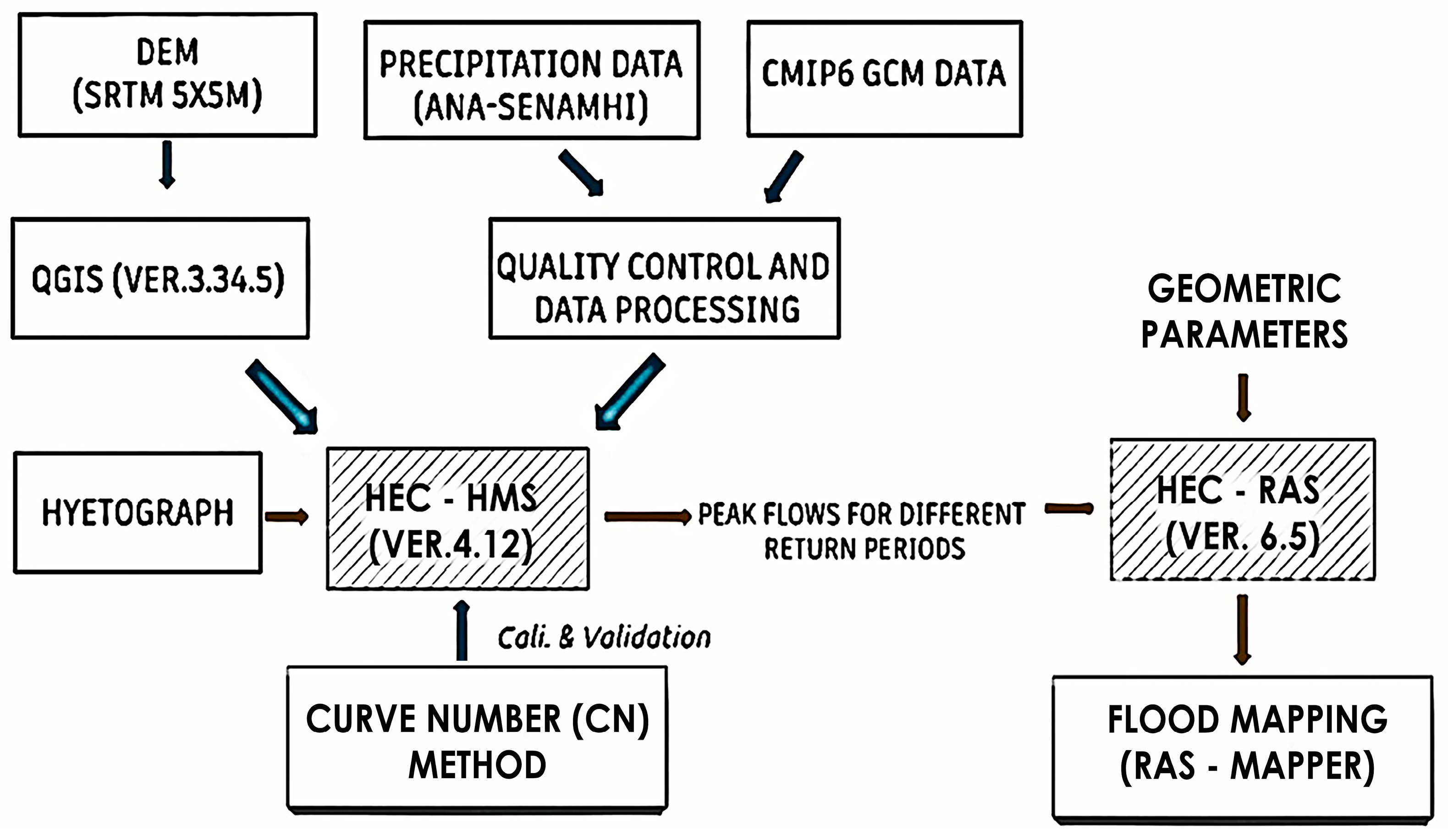
Figure 2.
Location and delimitation of the Cunas River Basin.
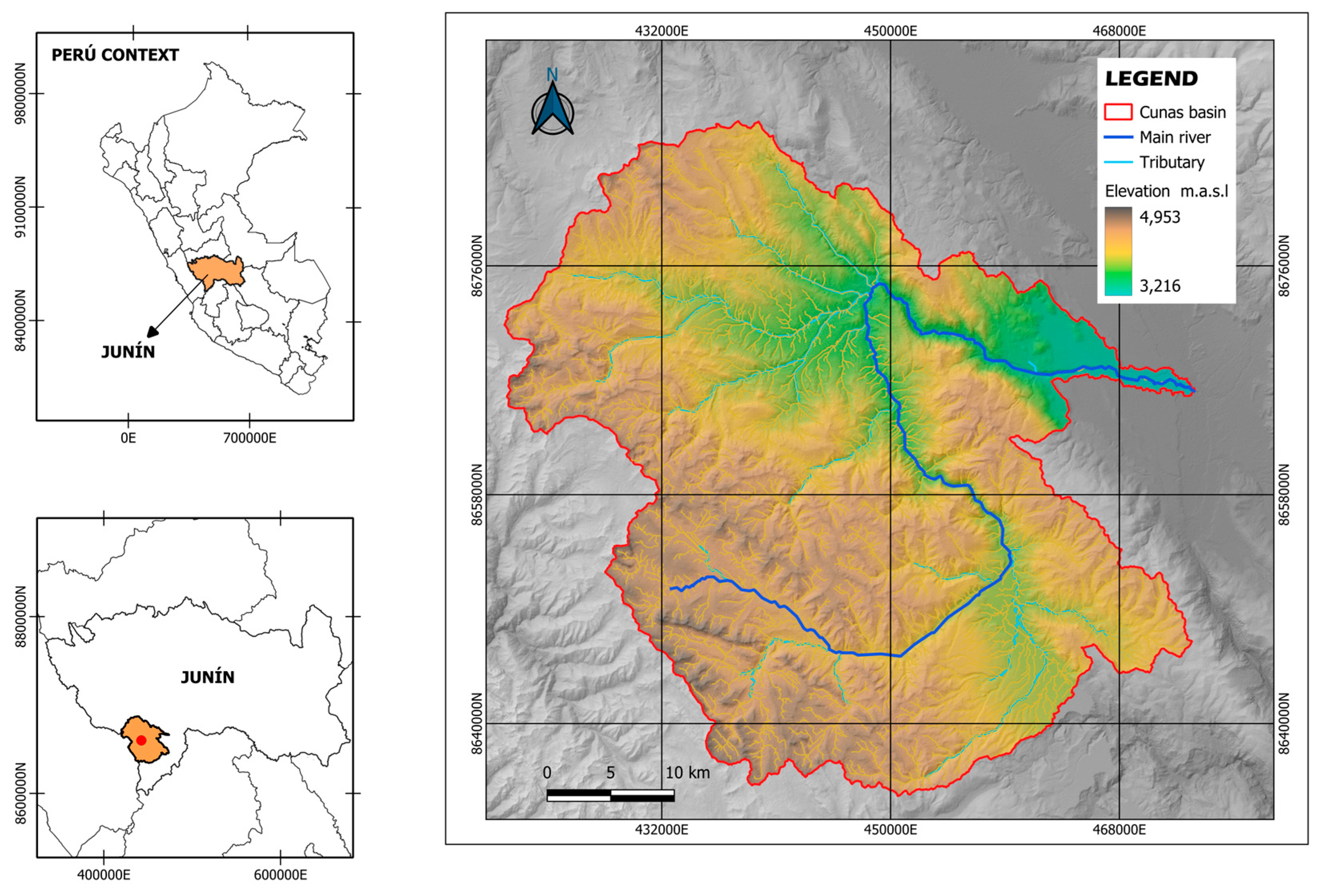
Figure 3.
Delimitation and surface area of the micro-watershed (analysis area).
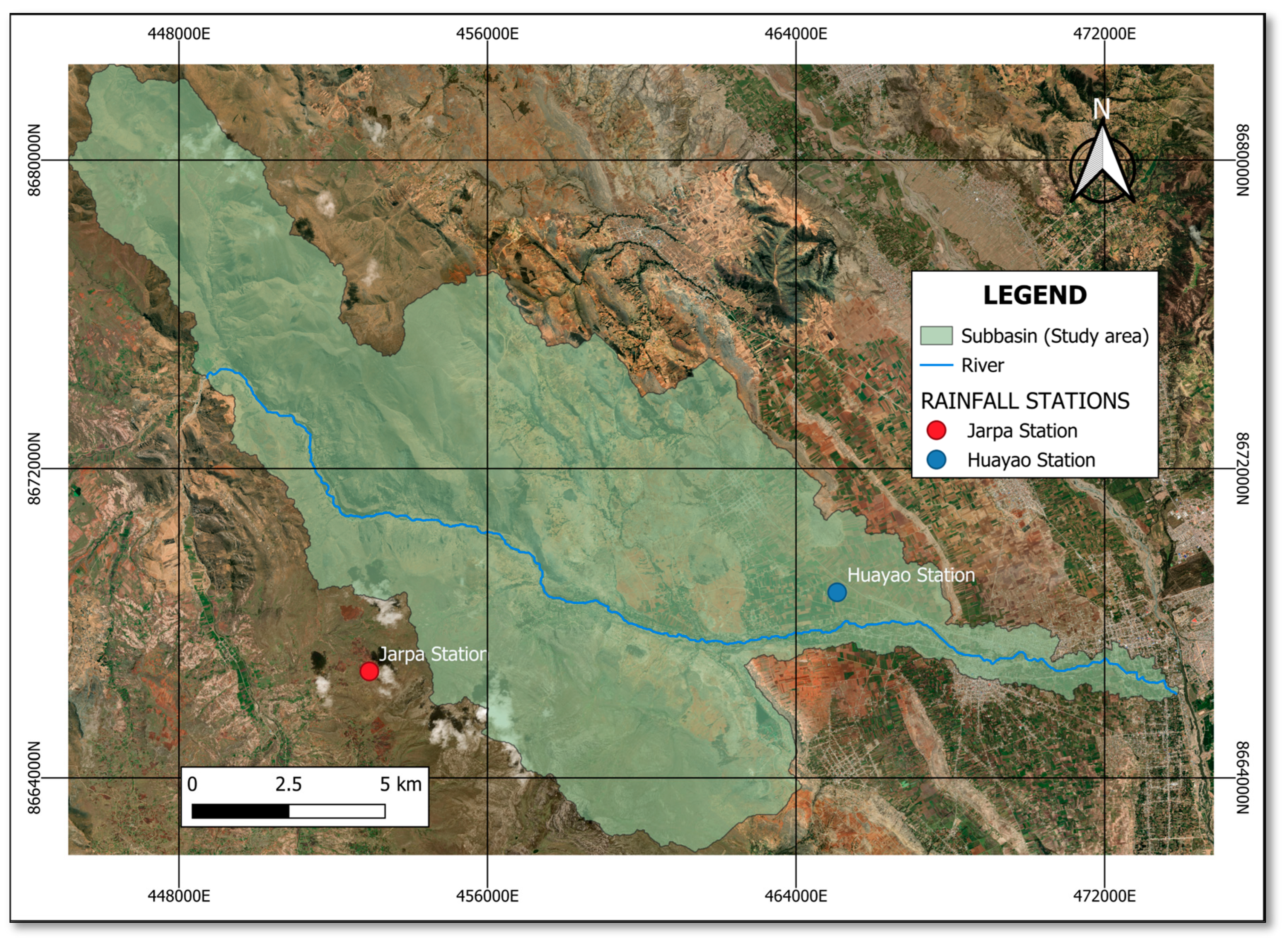
Figure 4.
Precipitation hyetograph for a 139-year return period under normal conditions.
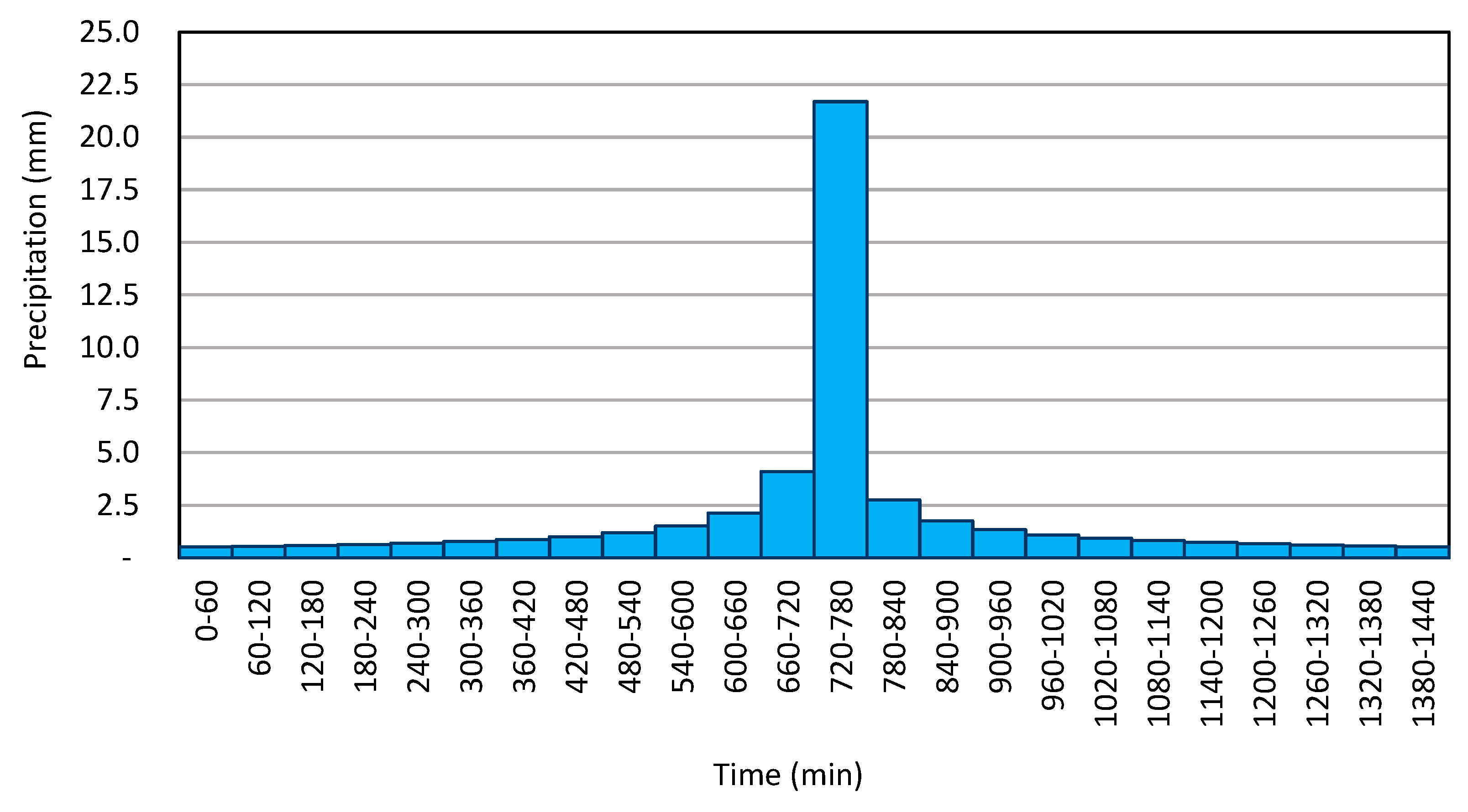
Figure 5.
Delimitation of river channel, delimitation for flood simulation and cross sections.
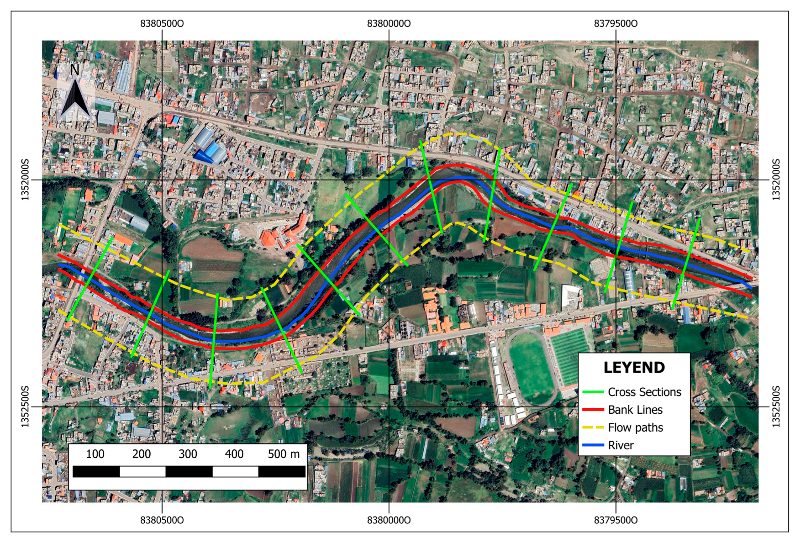
Figure 6.
Comparison between historical annual maximum daily rainfall and under the MultiModel Ensemble (MME).
Figure 6.
Comparison between historical annual maximum daily rainfall and under the MultiModel Ensemble (MME).
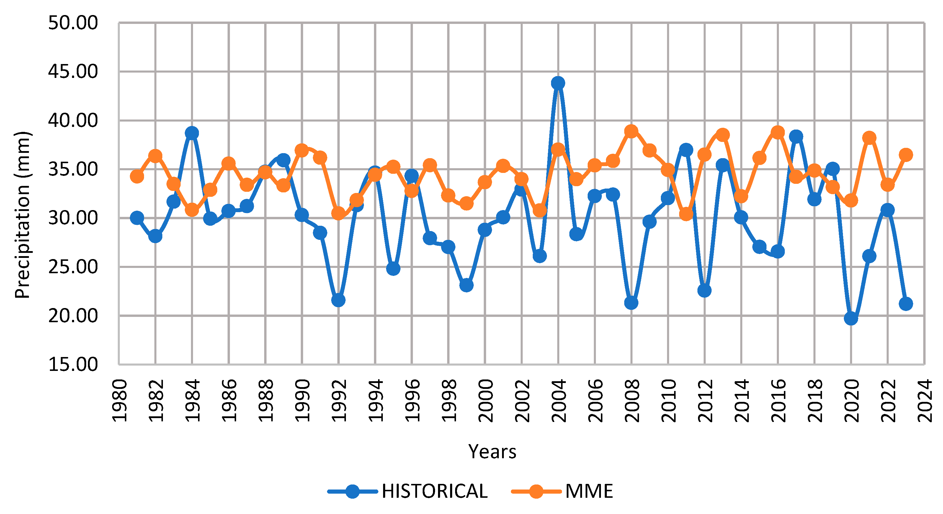
Figure 7.
Precipitation hyetograph for a 139-year return period influenced by climate change.
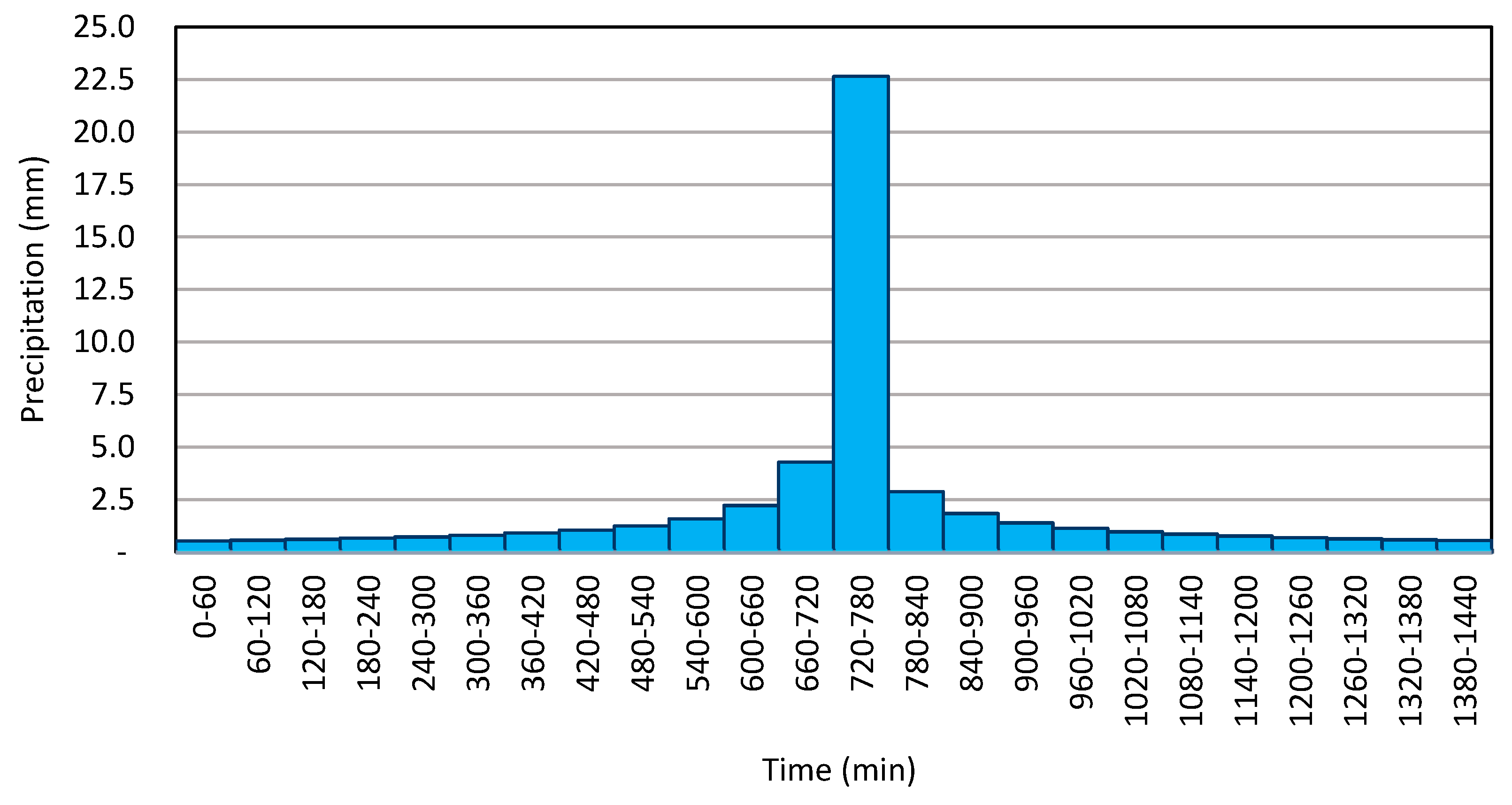
Figure 8.
Flow and time hydrograph for different return periods: (a) under normal conditions and (b) under the influence of climate change.
Figure 8.
Flow and time hydrograph for different return periods: (a) under normal conditions and (b) under the influence of climate change.
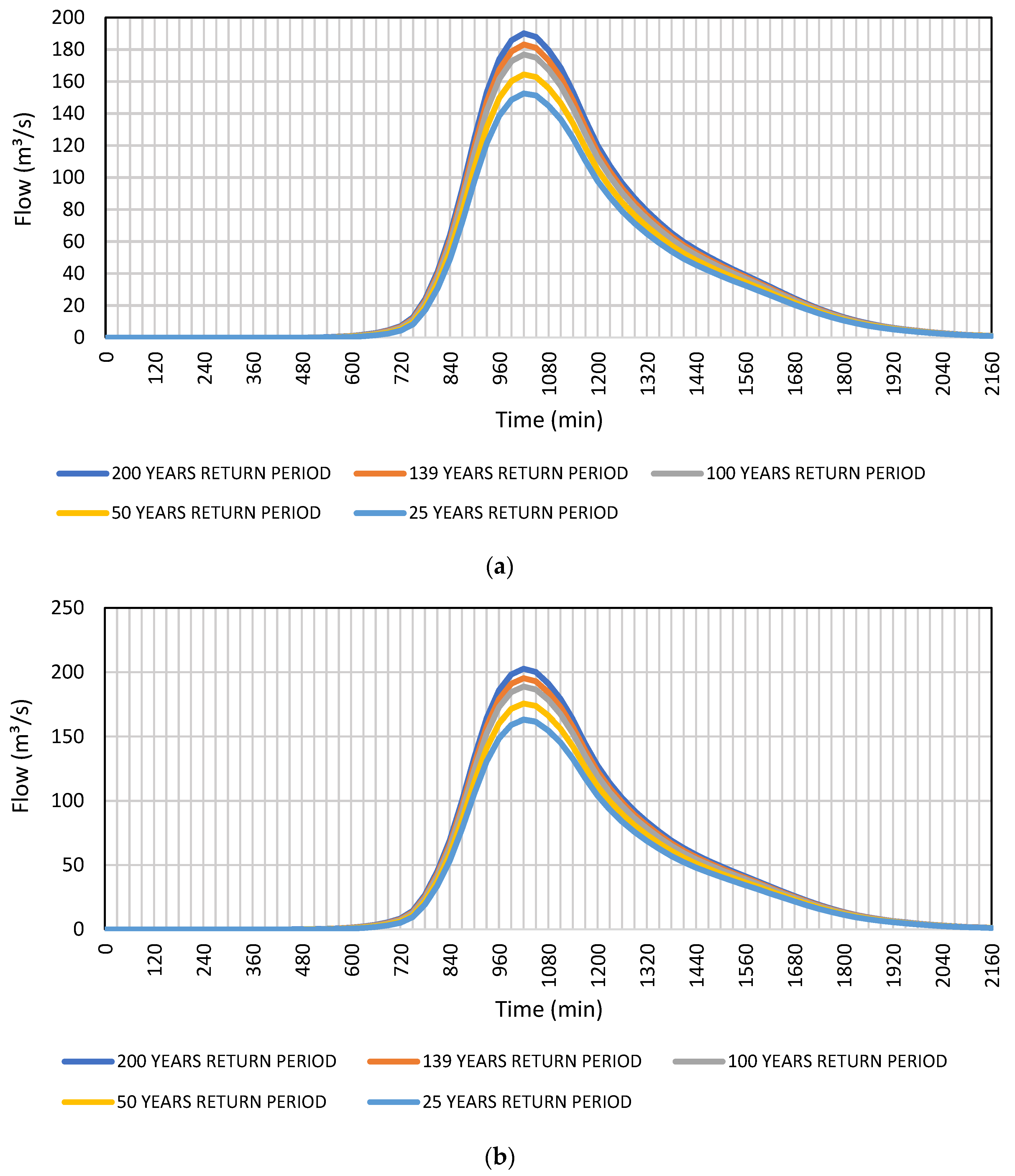
Figure 9.
Flood area and depth for a 139-year return period: (a) under normal conditions and (b) with the influence of climate change.
Figure 9.
Flood area and depth for a 139-year return period: (a) under normal conditions and (b) with the influence of climate change.
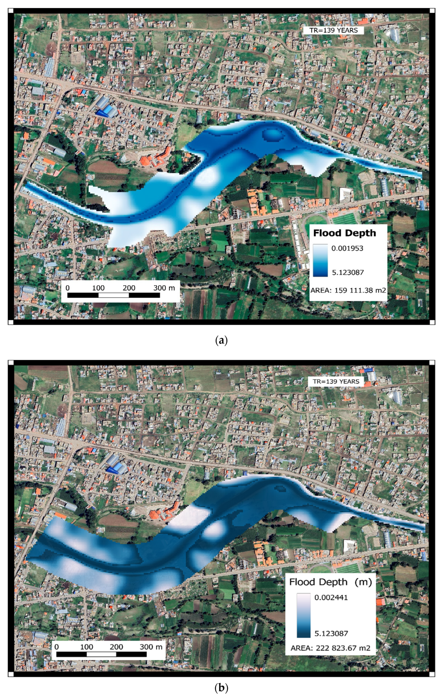
Figure 10.
Critical flood sections for a return period of 139 years: (a) under normal conditions and (b) with the influence of climate change.
Figure 10.
Critical flood sections for a return period of 139 years: (a) under normal conditions and (b) with the influence of climate change.
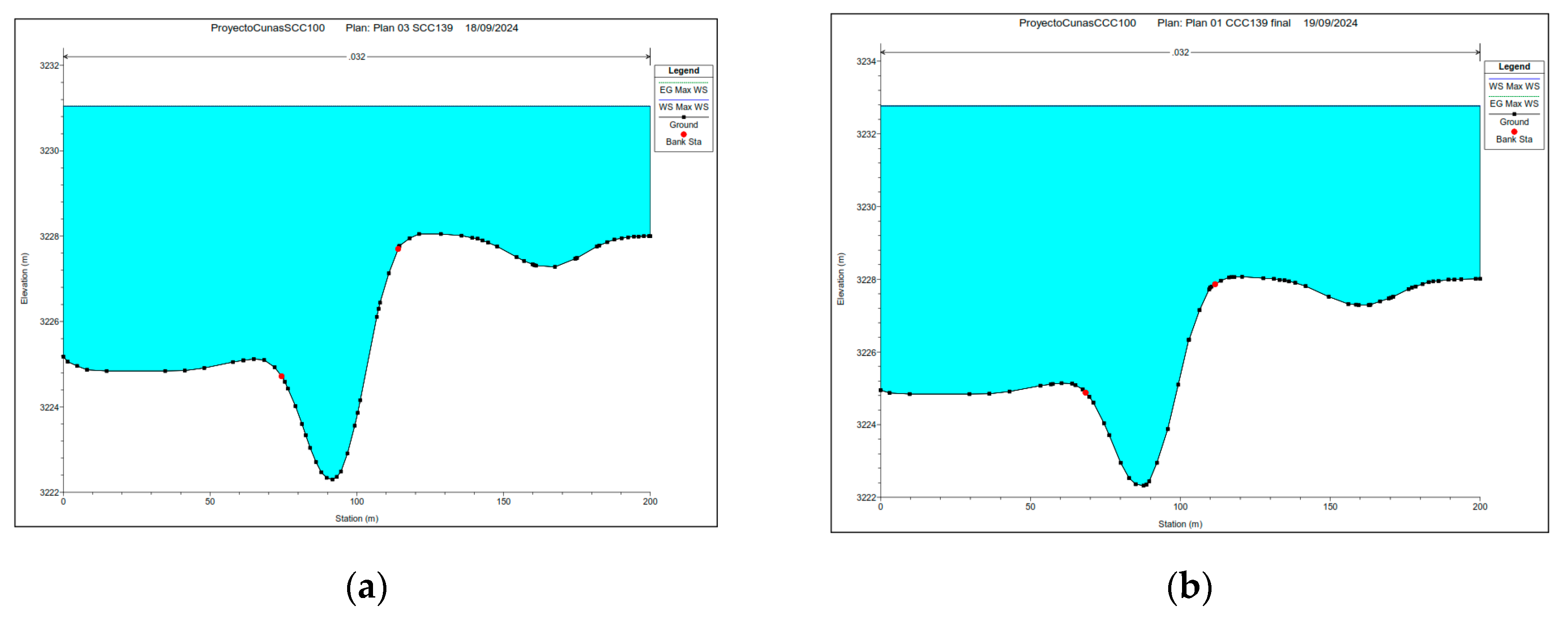

Table 1.
Main morphometric characteristics of the Cunas River basin.
| Cunas River Basin | Indicador | Unidad | Valor |
|---|---|---|---|
| Morphometric properties basin | Área | [Km²/s] | 1700.25 |
| Perímeter | [Km] | 279.62 | |
| Length | [Km] | 54.37 | |
| Width | [Km] | 31.27 | |
| Average slope | [%] | 23.73 | |
| Maximum elevation | [msnm] | 4953.00 | |
| Minimum elevation | [msnm] | 3216.00 | |
| Average elevation | [msnm] | 4203.82 | |
| Main channel properties | Length | [Km] | 93.79 |
| Length to the dividing line | [Km] | 98.50 | |
| Highest elevation | [msnm] | 4532 | |
| Lower elevation | [msnm] | 3221 | |
| Average slope | [%] | 1.40% | |
| Drainage network properties | Total length of drains | [Km] | 2839.16 |
| Drainage density | [Km/km²/s] | 1.67 | |
| Order of currents | [-] | 5° | |
| Runoff coefficient | [-] | 0.59 | |
| Form index | Compactness coefficient, Kc | [-] | 1.90 |
| Form factor, Kf | [-] | 0.19 |
Table 2.
Analysis of methods calculated for time of concentration
| Method used | Calculated Tc (Hrs) |
Var. Min (Hrs) | Var. Máx (Hrs) | Acceptance | Tc valid (Hrs) |
|---|---|---|---|---|---|
| Giandotti | 7.11 | 5.36 | 11.04 | Sí | 7.11 |
| Kirpich | 5.77 | 5.36 | 11.04 | Sí | 5.77 |
| California (U.S.B.R) | 5.78 | 5.36 | 11.04 | Sí | 5.78 |
| Témez | 9.62 | 5.36 | 11.04 | Sí | 9.62 |
| Johnstone Cross | 8.41 | 5.36 | 11.04 | Sí | 8.41 |
| SCS Ranser | 5.77 | 5.36 | 11.04 | Sí | 5.77 |
| Average Tc calculated for the hydrographic unit studied. | 7.08 | ||||
Table 3.
Comparison of maximum flows and volumes under the two conditions analyzed.
| Condition | Features | Return period (Years) | ||||
|---|---|---|---|---|---|---|
| 25 | 50 | 100 | 139 | 200 | ||
| Normal conditions | Precipitation volume (mm) | 42.62 | 44.72 | 46.93 | 48.01 | 49.24 |
| Volume of losses (mm) | 18.67 | 18.95 | 19.23 | 19.35 | 19.49 | |
| Excess volume (mm) | 23.95 | 25.77 | 27.7 | 28.66 | 29.74 | |
| Volume of direct runoff/desload (mm) | 23.90 | 25.72 | 27.65 | 28.61 | 29.69 | |
| Maximum flow (m³/s) | 152.50 | 164.40 | 176.90 | 183.10 | 190.10 | |
| With the presence of climate change | Precipitation volume (mm) | 44.51 | 46.7 | 49 | 50.14 | 51.42 |
| Volume of losses (mm) | 18.92 | 19.2 | 19.47 | 19.59 | 19.73 | |
| Excess volume (mm) | 25.58 | 27.5 | 29.54 | 30.54 | 31.69 | |
| Volume of direct runoff/desload (mm) | 25.54 | 27.45 | 29.48 | 30.49 | 31.63 | |
| Maximum flow (m³/s) | 163.20 | 175.60 | 188.80 | 195.30 | 202.70 | |
Disclaimer/Publisher’s Note: The statements, opinions and data contained in all publications are solely those of the individual author(s) and contributor(s) and not of MDPI and/or the editor(s). MDPI and/or the editor(s) disclaim responsibility for any injury to people or property resulting from any ideas, methods, instructions or products referred to in the content. |
© 2024 by the authors. Licensee MDPI, Basel, Switzerland. This article is an open access article distributed under the terms and conditions of the Creative Commons Attribution (CC BY) license (http://creativecommons.org/licenses/by/4.0/).
Copyright: This open access article is published under a Creative Commons CC BY 4.0 license, which permit the free download, distribution, and reuse, provided that the author and preprint are cited in any reuse.


