1. Introduction
Recently, flooding has become the most common and leading environmental hazard, with diverse impacts on human life, property, socioeconomic development, and agricultural production [
1,
2]. It is aggravated mostly by factors such as land use land cover (LULC) and climate changes [
3,
4]. LULC changes such as deforestation, agricultural expansion, and urbanization result in an increase in surface runoff by changes in the hydrologic characteristics of basins and watersheds [
5,
6]. While climate change causes flooding by changing the frequency, magnitude, and duration of extreme rainfall events [
7,
8,
9].
For projecting extreme rainfall events that would cause flooding, general circulation models (GCMs) available in the Coupled Model Intercomparison Project Phases 5 and 6 (CMIP5 and CMIP6) play a significant role [
10,
11]. However, these models are often associated with biases due to their coarse spatial resolution [
12]. To address this issue, the use of high-resolution downscaled outputs, such as those from the NASA Earth Exchange-Global Daily Downscaled Projections (NEX-GDDP) dataset, is generally recommended [
13,
14]. The NASA NEX-GDDP-CMIP5 and CMIP6 datasets provide daily temporal resolution and a spatial resolution of 0.25° (approximately 25 km × 25 km), making them suitable for watershed and basin scale studies [
15,
16]. Furthermore, the biases associated with climate models can be mitigated by evaluating and selecting the best-performing models, applying bias correction techniques, and using multi-model ensemble means of bias-corrected models [
17,
18,
19].
Historical LULC maps generated from remotely sensed images have been extensively used to assess past watershed and basin conditions [
3,
20,
21,
22]. Additionally, projected LULC maps under different scenarios are crucial for understanding future conditions. Consequently, several studies have focused on LULC predictions in different regions [
23,
24,
25]. For example, in the Gumara watershed, Belay et al. [
26] projected future LULC changes under a business-as-usual (BAU) and a governance (GOV) scenario. The BAU scenario assumes the continuation of current trends in land use change and socioeconomic development, whereas the GOV scenario incorporates the Green Legacy Initiative (GLI), a program currently being implemented by the Ethiopian government. Their study revealed significant expansion in cultivated land and settlements under the BAU scenario, whereas the GOV scenario predicted increases in forest, shrubland, and grassland. Similarly, a study by Gebresellase et al. [
27] in the upper Awash basin of Ethiopia reported the expansion of agricultural lands and urban settlements under the BAU scenario and improvements in forest cover under the GOV scenario.
Flood occurrence can be studied by estimating peak floods for different return periods. This is a crucial aspect in designing safe and cost-effective flood protection structures to minimize the destructive impacts of flooding on the environment [
28,
29,
30]. Return period-based peak floods can be estimated using statistical flood frequency analysis and hydrological rainfall-runoff models. The traditional statistical flood frequency analysis involves estimation of flood quantiles via a best-fitting probability distribution on the basis of the assumption that historical discharge time series are stationary and independent [
31]. However, rainfall-runoff hydrological models simulate the transformation of design storms (rainfall) into design floods, taking into account the effects of changing LULC and climate [
32,
33,
34].
Flooding mostly occurs at certain downstream reaches of the main river. Hence, before flood control structures are constructed, quantifying the contribution of upstream subwatersheds to the peak flood magnitude at the main outlet of the watershed is often recommended. This method is commonly known as flood source area identification (FSAI) [
35]. FSAI can be performed via multicriteria evaluation (MCE) and the unit flood response (UFR) approach [
36]. The MCE approach can be implemented via a geographic information system (GIS), which considers the linear combination of weights of several flood control factors [
37,
38]. However, this approach does not account for flow routing through rivers. The second approach, UFR, can be performed via hydrological models by accounting for flood routing through rivers for watersheds with diverse conditions [
36]. This method was first applied to the Damavand watershed in Iran by Saghafian & Khosroshahi [
35] and has since been used in various watersheds. For example, Abdulkareem et al. [
39] employed the UFR approach to assess the impact of LULC changes on FSAI for the Kelantan basin in Malaysia. In their study, the authors employed the Hydrologic Engineering Center-Hydrologic Modeling System (HEC-HMS) model and stated its importance for ranking subwatershed units on the basis of their contribution to peak discharge at the main outlet. Similarly, Fiorillo & Tarchiani [
40] applied this approach to a catchment in Niger and reported its suitability for identifying flood source areas.
Several studies conducted across various basins and watersheds have demonstrated a potential increase in high-flow extremes in future periods. These studies typically employed hydrological models to simulate future streamflow based on GCM outputs. For instance, Yang et al. [
41] assessed future changes in high-flow extremes in the Jiulong River Basin of Southeast China by simulating streamflow under changing LULC and climate conditions. Their findings indicated an increase in high-flow extremes due to intensified extreme rainfall and LULC changes driven by human activities. Similarly, Mahato et al. [
42] showed an increase in flood frequency in the Brahmani River Basin, India, by simulating streamflow using a semi-distributed hydrological model driven by outputs from CMIP6 models. In the Ethiopian context, Kassaye et al. [
43] showed a projected increase in high-flow extremes in the Baro River Basin by simulating streamflow using six GCMs under different scenarios. Likewise, Yalcin [
44] indicated a projected rise in flood frequency in Bitlis Creek, Turkey.
The downstream area of the Gumara watershed, particularly near Lake Tana, is one of the most flood-affected regions in the Upper Blue Nile (UBN) basin of Ethiopia [
45]. Several studies have addressed flood risk in this area through different approaches, including flood hazard mapping using the MCE method [
46], statistical flood frequency analysis [
30], hydraulic flood inundation modeling [
47], and flood mapping via Sentinel-1 images [
48]. However, return period-based peak flood estimation, FSAI, and extreme flow estimations under varying LULC and climate scenarios remain underexplored in the upstream region of the watershed. Additionally, most flood simulation studies in the Gumara watershed have relied on ground-based rainfall data. However, these observations often contain uncertainties due to missing data, sparse rain gauge networks, and the influence of topography [
49,
50]. To overcome these limitations, recent studies [
51,
52,
53] have suggested merging ground-based rainfall data with gridded rainfall products (GRFPs). This approach enhances the accuracy of flood simulations by reducing the uncertainties of ground-based rainfall measurements.
Hence, the objectives of this study are to (1) examine the impact of LULC change on return period-based peak floods and flood source areas (FSA) for the observation period (1981–2019) and (2) assess the combined impacts of LULC and climate change on high flow extremes, considering historical (1981–2005), near-future (2031–2055), and far-future (2056–2080) periods. To achieve these objectives, flood simulations were performed using a calibrated and validated HEC-HMS model.
For the observation period, the study utilized merged rainfall estimates from ground-based observed rainfall and three gridded rainfall products (GRFPs): Multi-Source Weighted-Ensemble Precipitation (MSWEP) [
54], Climate Hazards Group InfraRed Precipitation with Stations (CHIRPS) [
55], and the Enhanced Global Dataset for the Land Component of the Fifth Generation of European Reanalysis (ERA5-Land) [
56]. The merging process was performed using a random forest merging algorithm (RF-MERGE). LULC maps for the years 1985, 2000, 2010, and 2019 were incorporated alongside these merged rainfall estimates for this period.
To assess changes in high flow extremes between historical and future periods under changing LULC and climate conditions, high flow simulations were conducted using bias-corrected ensemble means of historical and projected rainfall data from four CMIP5 and four CMIP6 models. For the projected rainfall, the study accounted for representative concentration pathways (RCP4.5 and RCP8.5) for CMIP5 models and shared socioeconomic pathways (SSP2-4.5 and SSP5-8.5) for CMIP6 models. Additionally, future LULC scenarios under the BAU and GOV scenarios for 2035 and 2065 were considered for the near-future and far-future periods, respectively, alongside the future climate scenarios.
In summary, this study offers valuable insights into prioritizing flood source areas in the Gumara watershed and proposes targeted runoff reduction mechanisms. The estimation of high-flow extremes provides critical input for developing effective flood risk protection strategies, while the study’s methodology serves as a framework for flood simulations in similar watersheds across the UBN basin and beyond.
2. Materials and Methods
2.1. Study Area
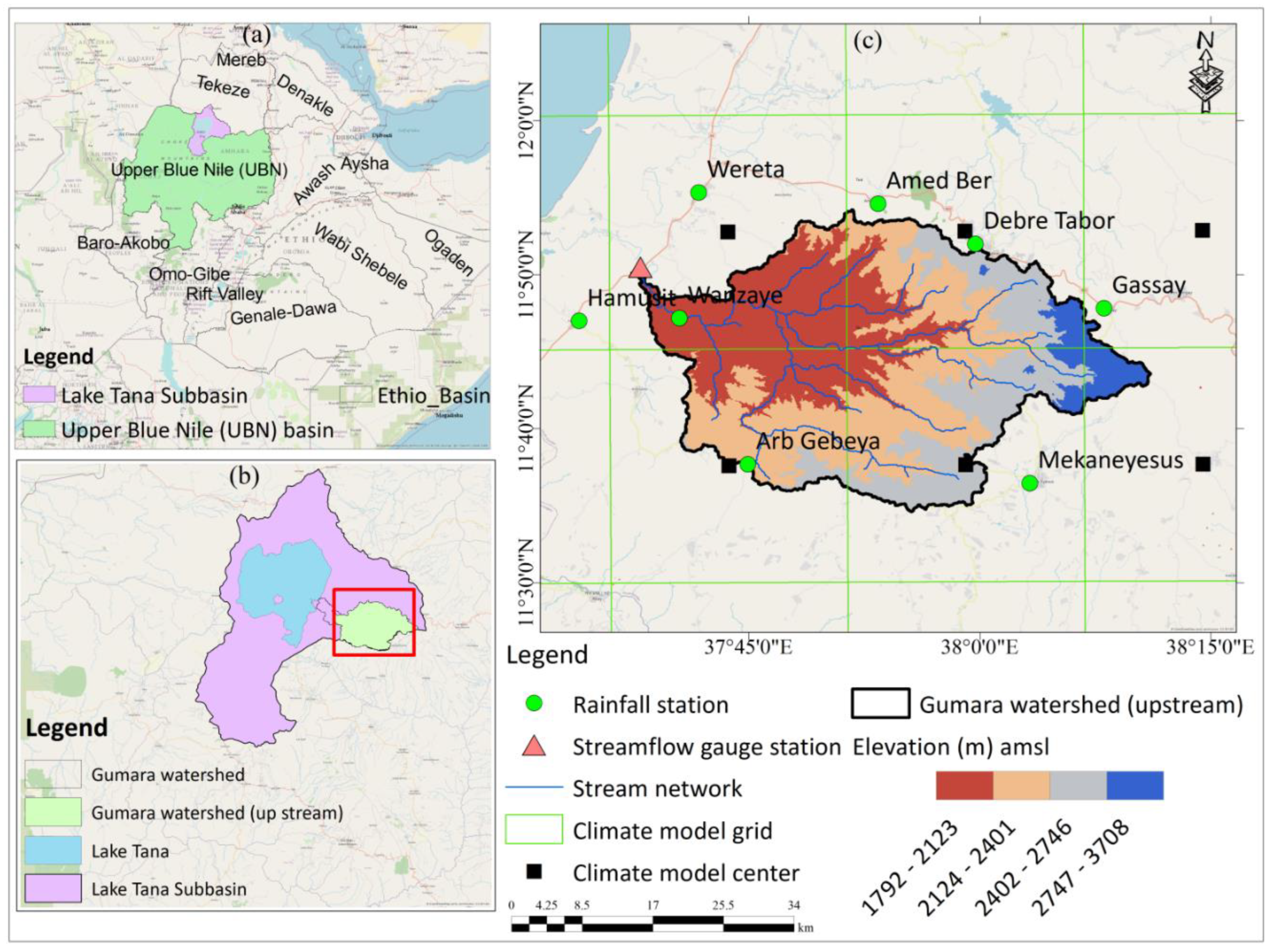
The Gumara watershed is part of the Lake Tana subbasin, which is located in the UBN basin of Ethiopia (
Figure 1). The watershed is primarily drained by the Gumara River, which originates from Guna Mountain. Geographically, it spans from 11° 35′ N to 11° 55′ N latitude and from 37° 35′ E to 38° 15′ E longitude. The drainage area of the watershed is approximately 1,256.7 km². The topography of the watershed is diverse, with elevations ranging from 1,792 to 3,708 m above mean sea level (amsl) (
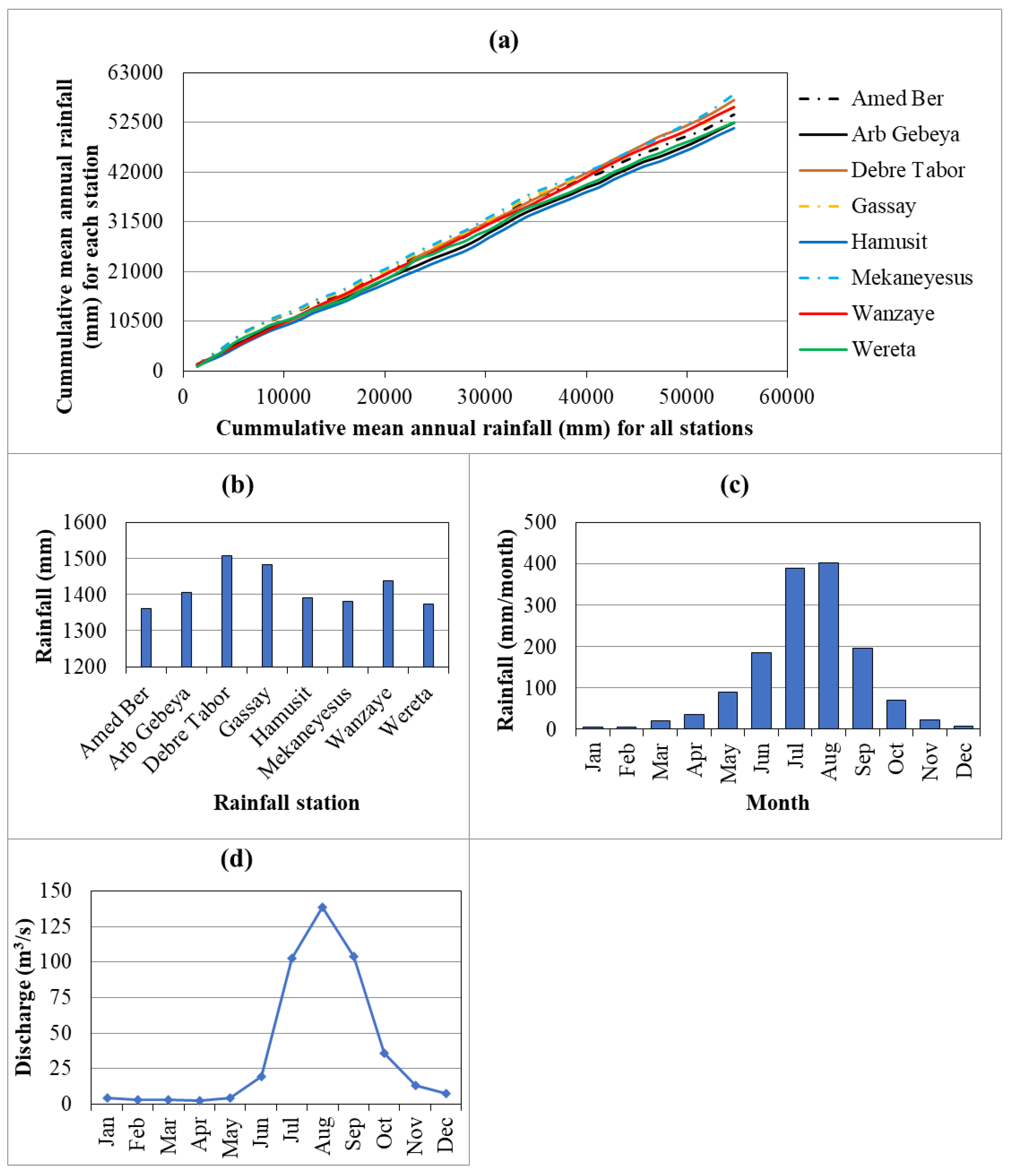
Figure 1c). It is characterized by steep gradients and mountainous terrain in its upstream areas and flat downstream floodplains. The watershed experiences a unimodal rainfall pattern, with the main rainy season occurring from June to September. The watershed receives an average annual rainfall of 1,445 mm, and its average annual temperature is about 20.5 °C [
57]. LULC in the watershed is dominated by cultivated land, which accounts for more than 80% of the total area, while the remaining portion of the watershed comprises forest, shrubland, grassland, and settlement areas [
26]. The predominant soil texture classes in the region include clay, clay loam, sandy clay, silty clay, and silty clay loam [
48]. The majority of the watershed is characterized by scattered rural settlements, where the local livelihood is primarily based on a mixed farming system (crop cultivation and livestock raising) [
58]. The downstream part of the watershed, which is adjacent to Lake Tana, is susceptible to frequent flood events due to high runoff generated from the upland watershed [
46,
59].
2.2. Data Used
For this study, various spatial and temporal data were collected from different sources. These include observed ground-based rainfall and streamflow, gridded rainfall products, climate model data, and spatial data such as elevation, soil, and LULC data.
2.2.1. Observed Ground-Based Rainfall and Streamflow Data
Ground-based daily rainfall data from eight meteorological stations located in and around the Gumara watershed were collected from the National Meteorological Agency (NMA) of Ethiopia, covering the long-term observation period from 1981 to 2019 (
Table 1).
The observed daily streamflow time series data (1981–2019) for the Gumara River at the Wanzaye gauging station were obtained from the Ministry of Water, Irrigation, and Electricity (MoIR) of Ethiopia. Selected events from this dataset were utilized for hydrological model sensitivity analysis, calibration, and validation.
2.2.2. Gridded Rainfall Products (GRFPs)
In watersheds with diverse topographies, such as the Gumara watershed, sparsely distributed meteorological stations may not adequately capture rainfall characteristics. To address this issue, three GRFPs were accessed and merged with ground-based observed rainfall. The three GRFPs selected for this study were MSWEP, CHIRPS, and ERA5-Land. MSWEP is a global gridded rainfall product that integrates multiple data sources, including satellite observations, gauge data, and reanalysis products, with a spatial resolution of 0.1° × 0.1° (approximately 10 km × 10 km). CHIRPS combines satellite-based infrared imagery with ground station data to provide a high-resolution rainfall product with a spatial resolution of 0.05° × 0.05° (approximately 5 km × 5 km). ERA5-Land provides high-resolution reanalysis rainfall data produced by the European Centre for Medium-Range Weather Forecasts (ECMWF), with a spatial resolution of 0.1° × 0.1° (approximately 10 km × 10 km). These GRFPs were selected due to their superior performance in reproducing the rainfall characteristics of the UBN basin [
60,
61]. For this study, CHIRPS and ERA5-Land at each ground-based station were accessed via the Climate Engine (
https://www.climateengine.org/), while the MSWEP dataset was extracted using a Python environment. For the three GRFPs, the time series data were accessed at a daily temporal scale for a common period (1981–2019).
Table 2 summarizes the spatial resolutions, access, and references for these datasets.
2.2.3. General Circulation Models (GCMs)
Historical (1981–2005), near-future (2031–2055), and far-future (2056–2080) rainfall data from four selected CMIP5 and four CMIP6 models were accessed from the NASA NEX-GDDP dataset. The time series rainfall data for these models were extracted for each ground-based meteorological station using a Google Earth Engine (GEE) sample script, available at this repository:
https://code.earthengine.google.com/74643b20363d1f0d4ee5875c456f5c14. For the CMIP5 models, future scenarios considered were RCP4.5 and RCP8.5, while for the CMIP6 models, SSP2-4.5 and SSP5-8.5 were utilized. The models were chosen on the basis of their better performance in reproducing historical extreme rainfall in the UBN basin following our recent work [
62]. All the CMIP5 and CMIP6 models are statistically downscaled outputs with a daily temporal resolution and 25 km x 25 km spatial resolution.
Table 3 summarizes detailed descriptions, including the resolutions of the climate models, modeling centers, and countries of the selected climate models. Details on the comparison and evaluation of the performance of the CMIP5 and CMIP6 models can be found in Belay et al. [
62].
2.2.4. Elevation, Soil, and LULC Data
The elevation data of the study watershed were extracted from a 30-meter spatial resolution digital elevation model (DEM) of the Shuttle Radar Topography Mission (SRTM) [
63]. The SRTM DEM data was accessed from USGS Earth Explorer via this link:
https://earthexplorer.usgs.gov/. The data was primarily used to generate subwatershed units and other watershed characteristics, including watershed slope and stream network.
Hydrologic Soil Groups (HSGs) for the study area were extracted from a 250-meter spatial-resolution soil grid map established by the USDA. The data was accessed via this link:
https://daac.ornl.gov/cgi-bin/dsviewer.pl?ds_id=1566. As shown in
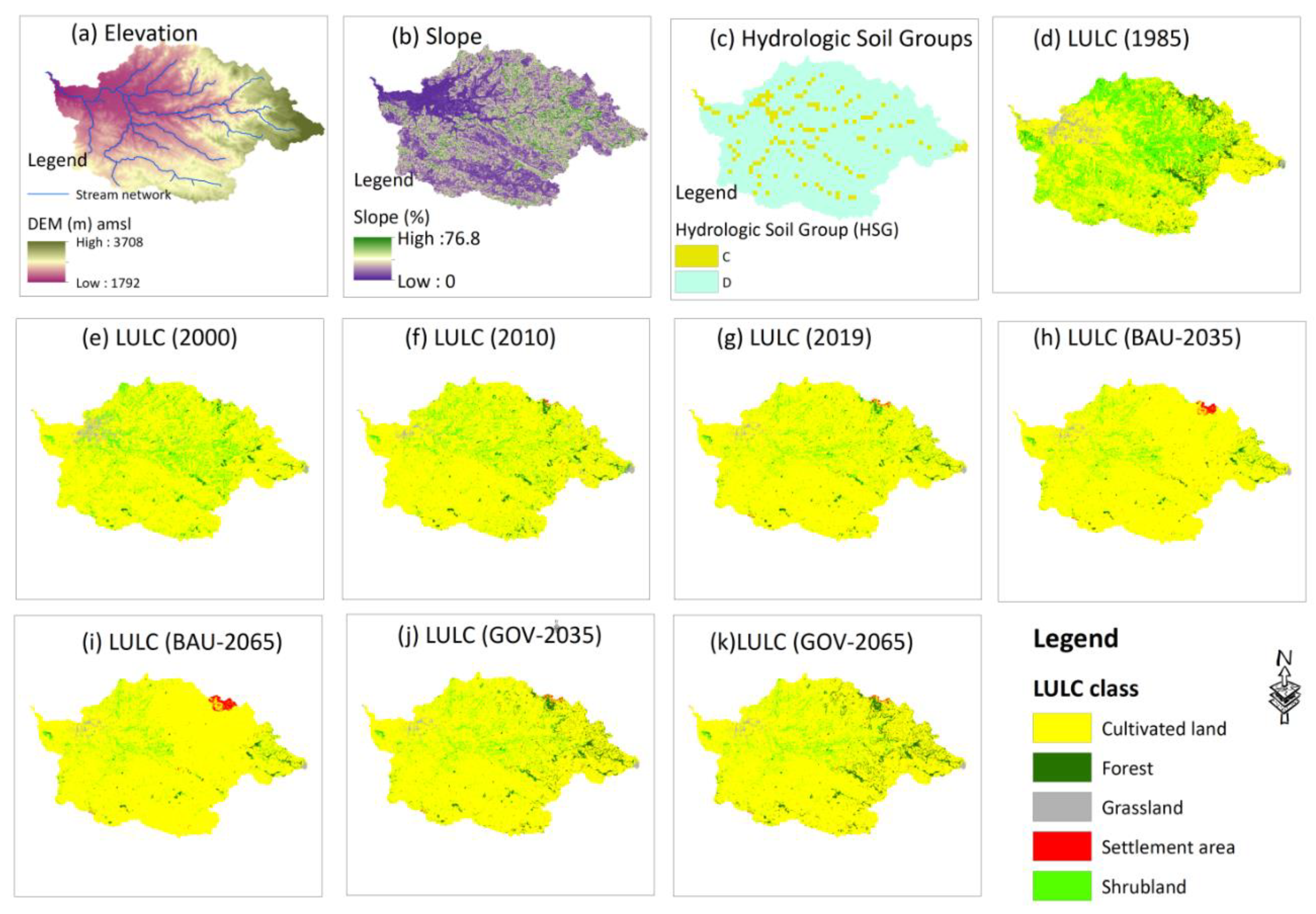
Figure 2c, HSG-D (clay loam, sandy clay, silty clay, silty clay loam, or clay) covers approximately 89% of the study watershed. These soils have high runoff potential because of very slow infiltration rates [
64]. The remaining portion of the study watershed is covered by HSG-C (sandy clay loam). These soils have a moderately high runoff potential due to slow infiltration rates [
64].
Raster files of historical and future LULC maps of the Gumara watershed, with a 30-meter spatial resolution, were clipped from our previous work [
26], which accounted for the entire Gumara watershed. In that work [
26], the LULC maps were generated using composite images from Landsat-5/Thematic Mapper (TM) for the years 1985, 2000, and 2010, and Landsat-8/Operational Land Imager (OLI) for the year 2019. For these years, cloud-free images from January to March were accessed from the U.S. Geological Survey via the GEE data catalog. LULC classification was performed using a Random Forest (RF) algorithm [
65] in the GEE environment, resulting in the identification of five dominant classes: forest, shrubland, grassland, cultivated land, and settlement areas, which describe the land use conditions of the study watershed. Specific information on the Landsat mission used, acquisition dates, and path/row details can be in the supplementary materials (
Table 1S).
In our previous work [
26], future land use prediction was performed via the Cellular Automata-Markov (CA-Markov) model available in the land change modeler (LCM) module of IDRISI Selva 17.0 [
66]. For the prediction, historical LULC maps (baseline) and various land-use change driver variables were considered, including elevation, slope, distance from roads, distance from streams, distance from towns, and socio-economic development (evidence of the likelihood of change). The prediction was conducted under two "what-if" scenarios: the Business-as-Usual (BAU) scenario and the Governance (GOV) scenario. The BAU scenario considered the current trend of land use conversion and change drivers (transition probability), whereas the GOV scenario accounted for the massive tree seedling plantation program of the Ethiopian government, known as the Green Legacy Initiative (GLI) program [
67].
Figures 2d-k show historical and predicted LULC maps of the Gumara watershed. Details on methods used for classification, accuracy assessment, LULC change drivers, scenario-based LULC prediction, and change detection for the entire Gumara watershed can be found in Belay et al. [
26].
2.3. Methods
This study analyzed peak floods for different return periods (5-, 10-, 25-, 50-, and 100-year) and flood source areas during the observation period (1981–2019) under varying LULC conditions. Additionally, high flow extremes were assessed for historical (1981–2005) and future (2031–2080) periods under different LULC and climate scenarios. The analysis involved collecting and processing spatiotemporal data, including daily ground-based rainfall, streamflow, GRFPs (MSWEP, CHIRPS, and ERA5-Land), CMIP5 and CMIP6 models, elevation, LULC, and soil data.
Ground-based rainfall data were merged with the three GRFPs using the RF-MERGE algorithm [
65] to enhance data accuracy. The merging process included four main steps: input data preparation, setting up the RF model, training the RF model, and performing the merging (prediction). For merging, ground-based rainfall data were used as the dependent variable, while GRFPs and other auxiliary data were used as independent variables. The resulting merged rainfall product was subsequently utilized in rainfall-runoff modeling, for extracting annual maximum (AM) 1-day rainfall series, and for correcting biases in climate model outputs. In the study, rainfall data from CMIP5 (MIROC5, MRI-CGCM3, CanESM2, and MPI-ESM1-2-LR) and CMIP6 (MPI-ESM1-2-LR, MRI-ESM2-0, CNRM-CM6-1, and BCC-CSM2-MR) models were also bias-corrected, and their ensemble means were predicted for historical and future periods to reduce uncertainties associated with climate models. Bias correction was performed using the quantile mapping (QM) method [
68]. From the corrected daily rainfall data, AM 1-day rainfall series were extracted and subsequently used to estimate high flow extremes in the near-future and far-future periods.
Flood simulation was conducted using the HEC-HMS model (version 4.11) [
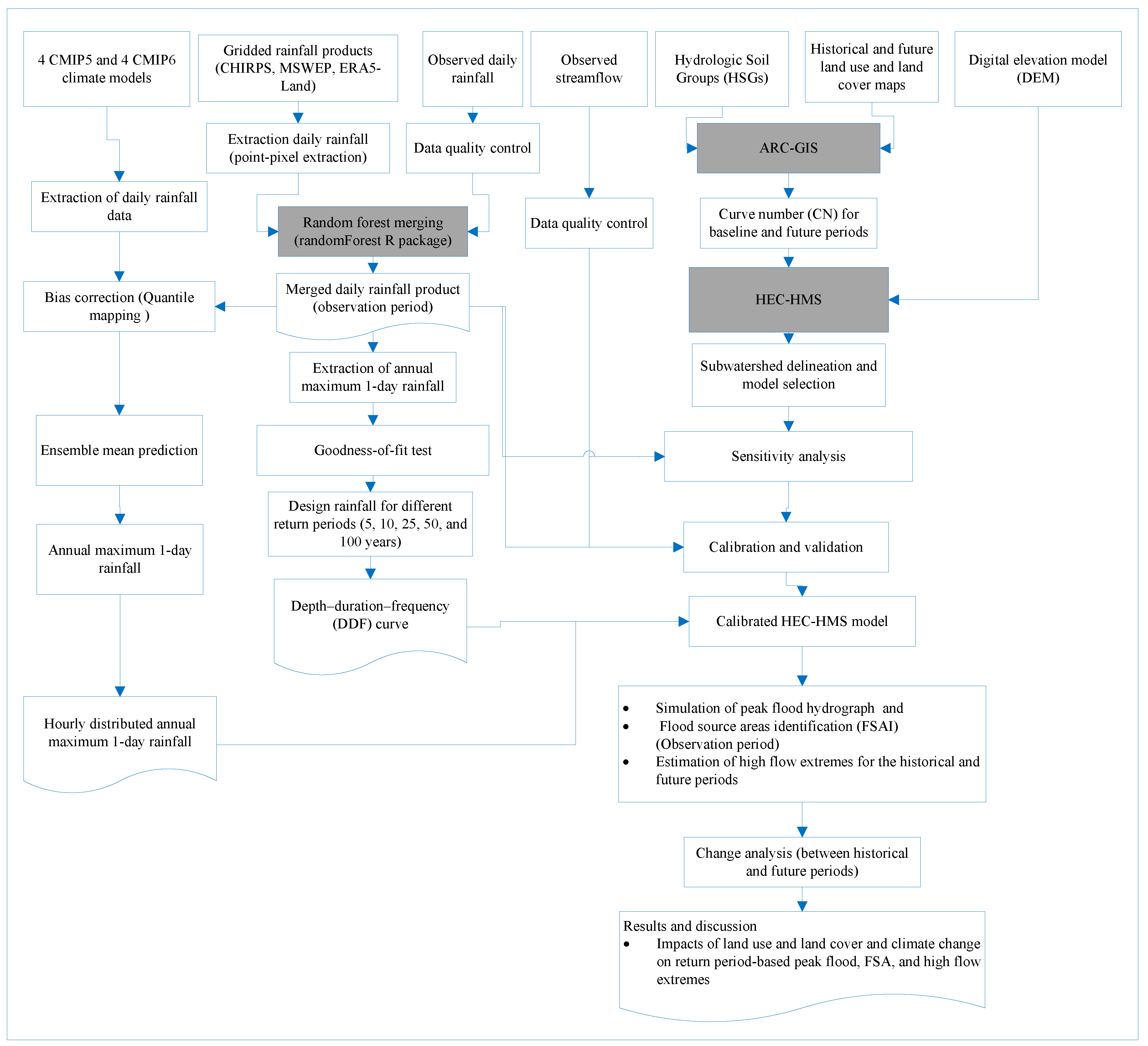
69]. The process included subwatershed delineation, entering rainfall data, model selection, parameter estimation and sensitivity analysis, calibration and validation, and flood simulation under various climate and LULC scenarios. Using the calibrated model, peak floods for different return periods were determined, flood source areas prioritized, and high flow extremes for historical and future periods assessed. The overall methodology is outlined in
Figure 3, with detailed explanations in subsequent sections.
2.4. Data Quality Control
In hydroclimatic studies, the use of long-term, homogeneous, and consistent data is generally recommended. However, the ground-based stations considered in this study have missing rainfall data and short-term rainfall records at the Hamusit, Wanzaye, and Arb Gebeya stations. The missing data were filled via the inverse distance weighting (IDW) technique, whereas short-term rainfall records were extended via the maintenance of variance extension, type 1 (MOVE.1) technique [
70]. After filling in missing data and extending short-term data, a homogeneity test was employed to detect change points in the mean annual rainfall data via the nonparametric Pettitt test [
71]. According to the Pettitt test statistics presented in the supplementary materials (
Table 2S), no significant changes were detected in the annual rainfall data for the stations considered in this study.
Double-mass curve (DMC) analysis was also employed to check the consistency of the mean annual rainfall data. This analysis involved inspecting significant changes in slope by plotting the cumulative mean annual rainfall of all stations on the x-axis and the cumulative mean annual rainfall of each station on the y-axis. From the analysis, all the stations were found to be consistent (
Figure 4a), since no significant changes in slope were detected in the DMC plot.
Figures 4b, c, and d also present mean annual rainfall at each ground-based station, mean monthly rainfall, and mean monthly discharge data, respectively.
2.5. Random Forest Merging (RF-MERGE)
To improve the quality of the rainfall data, the random forest (RF) merging approach (RF-MERGE) was employed to combine daily ground-based observed rainfall with three GRFPs (MSWEP, CHIRPS, and ERA5-Land). RF is a supervised machine learning algorithm that can be used for both classification and regression [
65]. Among the various merging approaches,
RF-MERGE was selected based on our previous work [
62], conducted in the study region. In that study, RF-MERGE demonstrated the best performance in reproducing observed rainfall compared to individual GRFPs and other merging approaches, as evaluated by both statistical and categorical performance measures. Additionally, RF-MERGE requires a minimal number of model parameters and is capable of handling high-dimensional data [
52].
For the merging process, ground-based rainfall data, three GRFPs, and auxiliary data (including date, month, year, and elevation) were first prepared. Next, the RF model was set up to map the relationship between the dependent and independent variables. In this study, ground-based rainfall data served as the dependent variable, while the three GRFPs, along with the auxiliary data, were used as independent variables. Subsequently, the RF algorithm was trained using rainfall data recorded at stations located in the UBN basin (
Table 3S in the supplementary materials). During training, the RF model learned the relationship between the dependent and independent variables. Based on this, the optimal parameter values of the RF algorithm, such as the number of trees (
), the minimum number of bootstrap samples (
), and the number of features (
) at the splitting node, were estimated. Finally, using the trained RF model, rainfall was predicted at stations located in and around the Gumara watershed (
Table 2). The merging procedure was performed via the "randomForest" R package [
72]. The analysis yielded estimated parameter values of 200, 6, and 3 for
,
, and
Nf, respectively. These parameters were determined through trial-and-error procedures and by comparison with parameters estimated in previous studies [
73,
74]. Using these parameters, the trained model was subsequently used to predict daily rainfall at the eight testing stations. The merged rainfall data were then used to extract the AM 1-day rainfall, correct the bias of the climate models, and calibrate/validate the hydrological model. A comprehensive review, including assumptions, procedures, and limitations of various merging approaches, such as RF-MERGE, can be found in our previous work [
50].
2.6. Design Rainfall and Depth‒Duration‒Frequency (DDF) Curve
In this study, the annual maximum 1-day rainfall data series for the observation period (1981-2019) was extracted and fitted to commonly used probability distributions: normal (NOR), lognormal (LN3), gamma (GAM), Gumbel (GUM), Pearson type III (PE3), log Pearson type III (LPE3), and generalized extreme value (GEV) distributions. The parameters of these distributions were calculated via the L-moments method provided in Hosking & Wallis [
31]. The Anderson‒Darling (AD) test [
75] was employed to assess goodness-of-fit by comparing the CDFs of the observed data with those of the candidate distributions. This test is sensitive to deviations in the tails of the probability distribution, making it valuable for applications involving extreme values [
76]. The best-fit distribution was selected on the basis of the lowest AD statistic (
) at the 5% significance level and used for estimating design rainfall for different return periods.
To simulate flood hydrographs for different return periods (5-, 10-, 25-, 50- and 100-year), a short-duration (example with an hourly distribution) depth‒duration‒frequency (DDF) curve is often needed. For this, a short-duration hourly distributed DDF curve was developed using the following equation:
where
is the computed rainfall depth for a duration of
t hours,
is the design rainfall depth for a 24-hour (1-day) duration,
is the rainfall duration in hours,
is a parameter that controls the relationship between different durations and can be determined on the basis of regional studies, and
is an exponent that adjusts the amount at which rainfall decreases with shorter durations and can be determined empirically on the basis of regional studies. For this study, the DDF curve for a 1-hour duration was developed using 0.3 for the parameter
and 0.9 for the exponent
following regional studies conducted in Ethiopia [
77,
78].
2.7. Bias Correction
It is common for climate model simulations to exhibit bias (uncertainties) due to their coarse spatial resolution, model assumptions, boundary conditions, spatial averaging, and other factors [
79,
80]. To address this issue, it is generally recommended that biases in climate models be corrected before their outputs are applied in impact assessment studies [
81]. Among the different types of bias correction methods, the QM approach was used in this study because of its better performance in the study region [
62]. The QM method uses the quantile‒quantile relationship to match the distribution function of climate model simulations with observed data [
68]. The method assumes that the cumulative distribution functions (CDFs) of the observed and simulated datasets can be matched, meaning that the CDFs of the observed and simulated data should be similar enough for meaningful bias correction [
82]. Based on this assumption, for a given simulated value
, QM bias correction adjusts it using:
where is bias corrected value, is CDF of the simulated data, is CDF of the observed data, and is inverse CDF (quantile function) of the observed data.
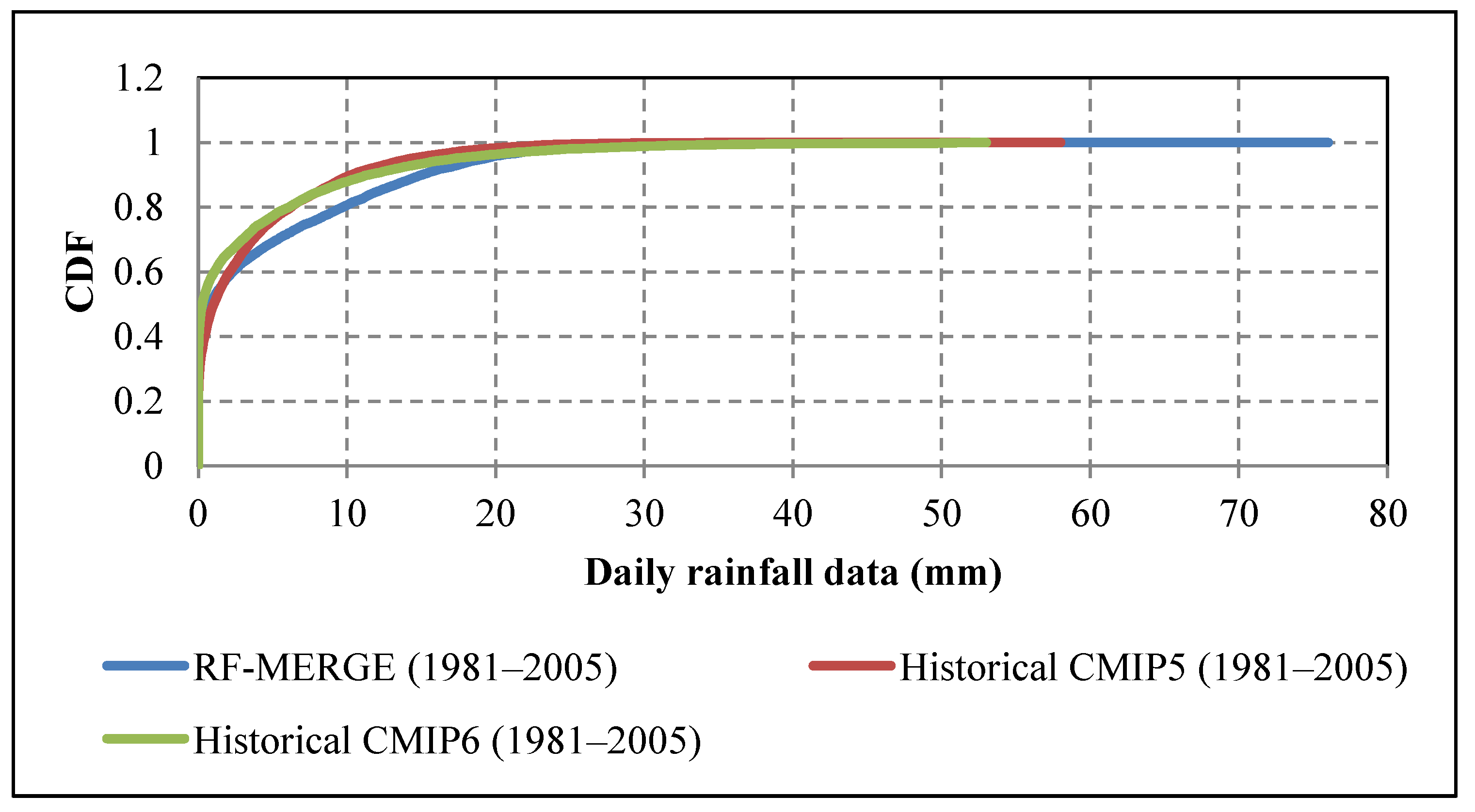
In this study, prior to implementing QM bias correction, the CDFs of daily observed rainfall from RF-MERGE and simulated rainfall from historical CMIP5 and CMIP6 were computed and plotted, as shown in
Figure 5, to assess their similarity. The graph indicates that the CDFs of the observed and simulated data are sufficiently similar, allowing the QM method to be applied.
Among the different types of QM approaches, the parametric transformation function (PTF) was chosen for this study because of its effectiveness in studying extreme rainfall events [
83]. The bias correction was applied by matching the historical climate model data with the RF-MERGE data and then applying the correction to the future climate model data on the basis of historical relationships. A detailed explanation of the assumptions and formulations of the various QM bias correction methods can be found in Enayati et al. [
82].
2.8. Rainfall-Runoff Modeling
Rainfall-runoff modeling can be conducted using various distributed and semi-distributed hydrological models. According to Ghonchepour et al. [
84], factors such as modeling objectives, hydrologic conditions, limitations, assumptions, and data availability should guide model selection. In this study, the HEC-HMS model was chosen for its suitability in simulating rainfall-runoff processes under varying LULC and climatic conditions, aligning well with the study's objectives. HEC-HMS is a physically based, semi-distributed model widely recognized for its effectiveness in flood modeling [
85,
86,
87]. It is compatible with the input data used in this study, including rainfall, streamflow, LULC, soil, and DEM data. Its semi-distributed structure facilitates accurate flow simulation at the subwatershed scale, which is critical for identifying flood source areas. Furthermore, HEC-HMS has been thoroughly tested and shown to perform well in modeling floods in similar watersheds within the UBN basin of Ethiopia [
88,
89].
The HEC-HMS model consists of several key components (managers), including basin models, meteorological models, time-series data, and control specifications [
69]. The basin model defines the physical characteristics of the watershed, such as subwatersheds, river reaches (networks), junctions, outlets, and others, along with relevant hydrological parameters. The meteorological model specifies the type of rainfall data used in the simulation. The time-series data component is used to input rainfall and streamflow data, which are essential for driving the model. Lastly, control specification manages or sets the simulation time step, duration, and output intervals. These components work together to simulate hydrologic processes and provide flood hydrographs.
In this study, rainfall-runoff simulations in the HEC-HMS model involved subwatershed delineation (basin model), entering rainfall and streamflow data, model selection (for runoff volume, direct runoff, and routing), parameter estimation and sensitivity analysis, model calibration and validation, and flood hydrograph simulations under changing LULC and climate conditions as detailed in the subsequent sections.
2.8.1. Subwatershed Delineation
Subwatershed delineation was performed using a 30-meter resolution SRTM-DEM via the GIS tools in HEC-HMS 4.11, as this version is integrated with GIS components. The process involved setting up the coordinate system (projection), terrain reconditioning, filling sinks, drainage line processing, identifying streams, defining outlets, and delineating subwatersheds. Since the middle and upper portion of the Gumara watershed lies in steep gradient areas (slope greater than 15%), the 30-meter DEM resolution could introduce inaccuracies, particularly in calculating flow direction and accumulation. These limitations may result in misrepresentation of the river network of the watershed. To address this issue, DEM reconditioning techniques, such as stream burning and sink filling, were applied to improve the representation of hydrological features. Additionally, during subwatershed delineation, the homogeneity of various watershed characteristics, such as soil, LULC, elevation, and stream networks, was considered for merging similar smaller subwatersheds into one.
2.8.2. Rainfall and Streamflow Data
This study utilized daily rainfall data from RF-MERGE (1981–2019), rainfall DDF curves for return periods of 5, 10, 25, 50, and 100 years, and rainfall for both historical and future periods to simulate streamflow. Observed streamflow data for the Gumara River (1981–2019) were also employed to compare with simulated flows during model calibration and validation, focusing on selected flood events.
2.8.3. Model Selection
In the HEC-HMS, there are various models for computing runoff volume, direct runoff, and channel flow routing. For this study, the Soil Conservation Service Curve Number (SCS-CN) [
90], SCS unit hydrograph (SCS-UH) [
90], and Muskingum channel routing [
91] models were selected for modeling runoff volume, direct runoff, and channel flow routing, respectively.
- I.
Modeling runoff volumes (loss model)
Models available in the HEC-HMS generally compute runoff volume by subtracting the sum of various losses from the accumulated rainfall. Among these models, the Soil Conservation Service Curve Number (SCS-CN) method was selected for this study because it can compute runoff volume for a given rainfall event as a function of HSGs, LULC, and antecedent soil moisture conditions.
In the SCS-CN model, the excess rainfall (
) at a given time
is the rainfall in excess of the infiltration capacity and other losses and can be computed as:
where
is the accumulated rainfall depth at time
;
is the initial abstraction (loss); and
is the maximum retention potential of the watershed. Considering the analysis findings from many experimental watersheds, the SCS-CN provides an empirical relationship of
and
, which is given as
.Then, the expression of
at a given time
becomes:
The maximum retention (
) can be computed as a function of the CN via the following equation.
In this study, 30-m spatial resolution gridded runoff CN maps were generated by considering soil and LULC characteristics (raster files), as well as the average antecedent moisture conditions (AMC-II). For the soil moisture condition, the AMC-II was accounted for because it represents a standard condition commonly used in hydrological modeling. The gridded CN maps were prepared via the ARC-GIS 10.4 environment [
92]. The process involved preparing input data by aligning raster files (LULC and soil) to the same resolution, coordinate system, and extent; reclassifying LULC and HSG maps; combining them; and assigning curve numbers using a lookup table with a raster calculator.
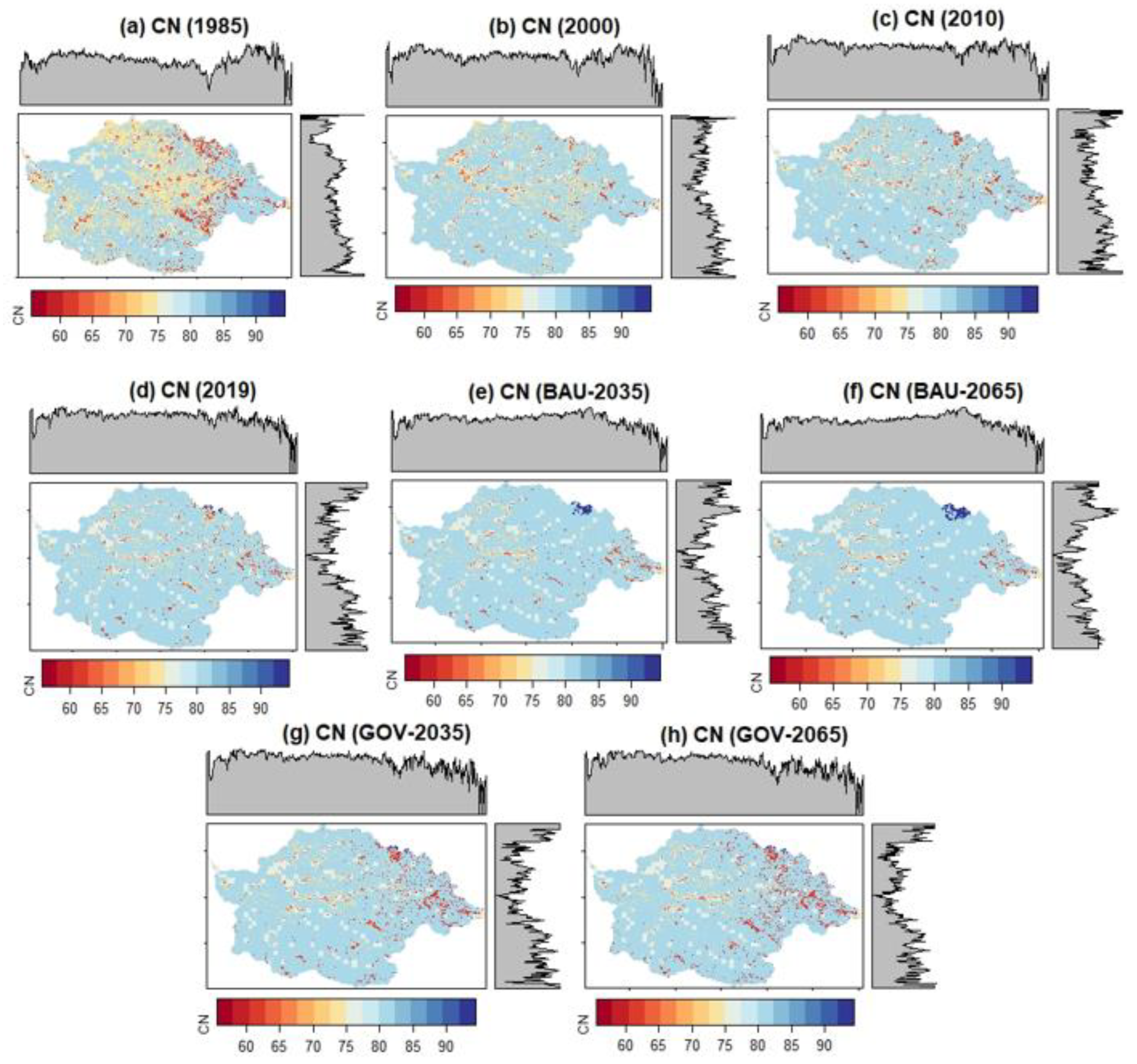
Figure 6 shows the gridded runoff curve numbers for both the historical and future periods generated based on these procedures. The results indicate that the CN values under the BAU scenario are relatively greater than those under the governance (GOV) scenario. This is attributed to the expansion of cultivated land and settlement areas under the BAU scenario. As a result, the maximum retention potential of the watershed will reduce, which may lead to an increase in peak flow occurrence due to higher surface runoff volumes. The composite CN for each subwatershed was estimated on the basis of the mean value of raster grids (pixels) within the boundaries of the subwatershed area. Similarly, the composite CN for the entire watershed was calculated as the mean value of raster grids within the boundary of the whole watershed.
- II.
Direct runoff (transform model)
In the HEC-HMS model, several empirical and conceptual models are available to transform excess rainfall into direct runoff. Among these, the SCS unit hydrograph (SCS-UH) model [
90] was selected for this study. The key parameter of this model is the lag time (
), which represents the time difference between the center of mass of excess rainfall and the peak of the SCS-UH. Although the assumption of a single-peak hydrograph is a limitation of the SCS-UH, it was chosen because its parameters can be estimated from the physical characteristics of the watershed, specifically in relation to the time of concentration
. For this model,
can be computed via the Kirpich equation [
93], and
is then calculated as 0.6 times
:
where
is the time of concentration (minutes),
is the length of the longest flow path (meter), and
is the average channel slope (m/m).
- III.
Channel flow (routing model)
From the available flow routing models in the HEC-HMS model, the Muskingum routing model was selected for this study. This model uses a finite difference approximation of the continuity equation and is widely used for flood routing [
94]. It accounts for flow attenuation resulting from the storage effect of the channel as flood flows travel through it.
The Muskingum routing model computes channel storage as follows:
where
,
, and
are storage, inflow, and outflow at time
, respectively;
is the travel time of the flood wave though the routing channel; and
is a dimensionless weight factor (
For this study, the Muskingum routing model parameters (
and
) were determined through model calibration.
2.8.4. Model Sensitivity Analysis
Sensitivity analysis is a critical step in hydrological modeling aimed at reducing uncertainty and identifying model parameters that significantly influence the model's output [
86,
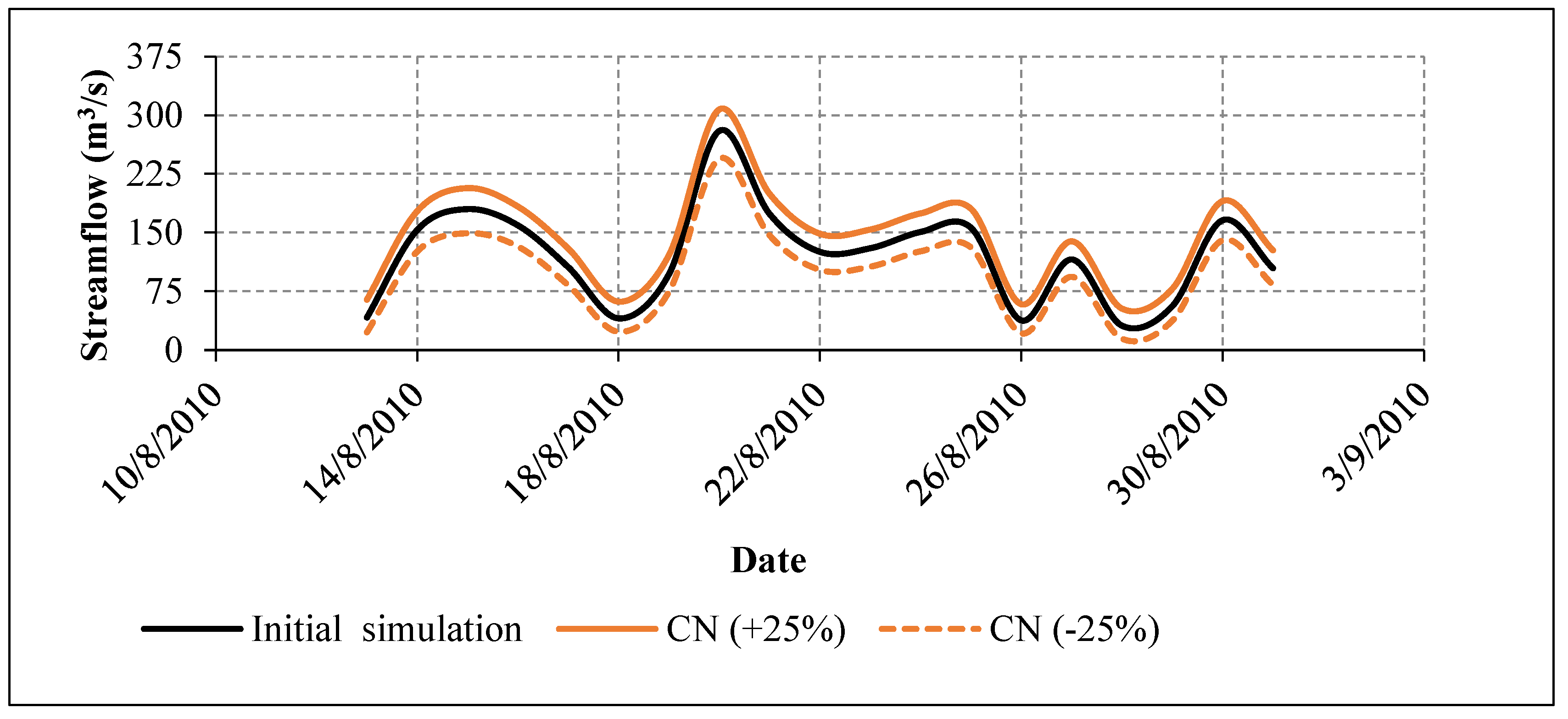
95]. In this study, sensitivity analysis was conducted for the parameters of the runoff volume (loss) and transform models by varying each parameter individually while keeping the others constant (local sensitivity analysis). Each parameter value was adjusted by ±25%, and the relative percentage change in peak discharge was assessed for each simulation. The sensitivity of each parameter was evaluated on the basis of the magnitude of the change in peak flow. The relative change in peak flow as a percentage was computed via the following equation:
where is the peak flow after changing the parameter and where is the peak flow from the baseline simulation. In this study, model sensitivity analysis was performed for selected events that occurred from 13 to 31 August 2010.
2.8.5. Model Calibration and Validation
Model calibration and validation were performed to match the observed and simulated data for selected events. Both automated and manual calibrations were employed to obtain better agreement between the simulated and observed flow events through iterative adjustments of the model parameters. The performance of the model during calibration and validation was evaluated through graphical comparison (visual comparison) and statistical performance measures such as the coefficient of determination (
), Nash–Sutcliffe efficiency (
), root mean square error (
), and percent bias (
). These performance measures were selected from different categories:
from standard regression-based methods,
from dimensionless methods, and
and
from error-based statistical methods [
96].
expressed in equation 9 describes the proportion of the variance in the observed data explained by the model-simulated data.
where
is the
observed discharge value for the event being evaluated,
is the
simulated discharge value for the event being evaluated,
is the mean of the observed discharge values,
is the mean of the simulated discharge values, and
is the total number of observations.
values range from 0 to 1 (inclusive), with higher values indicating less error variance, and values higher than 0.5 are generally considered acceptable values [
97].
The NSE is a dimensionless statistical performance measure that describes the relative magnitude of the residual variance (noise) compared with the observed data variance (information) [
98].
is expressed as shown in equation 10:
ranges from to , where indicates good agreement between the observed and simulated values, is generally considered acceptable, and indicates poor or unacceptable model performance.
expressed in equation 11 describes the standard deviation of the model prediction error.
The optimal value of is 0, which indicates perfect agreement between the observed and simulated values.
where
indicates the average tendency of the model-simulated values to be higher or lower than the observed values [
99]. It is given as shown in equation 12:
The optimal value of
is 0, with low values indicating accurate model simulation. Positive
values indicate overestimation, whereas negative values indicate model underestimation. According to Moriasi et al. [
100],
is an acceptable range for discharge simulation.
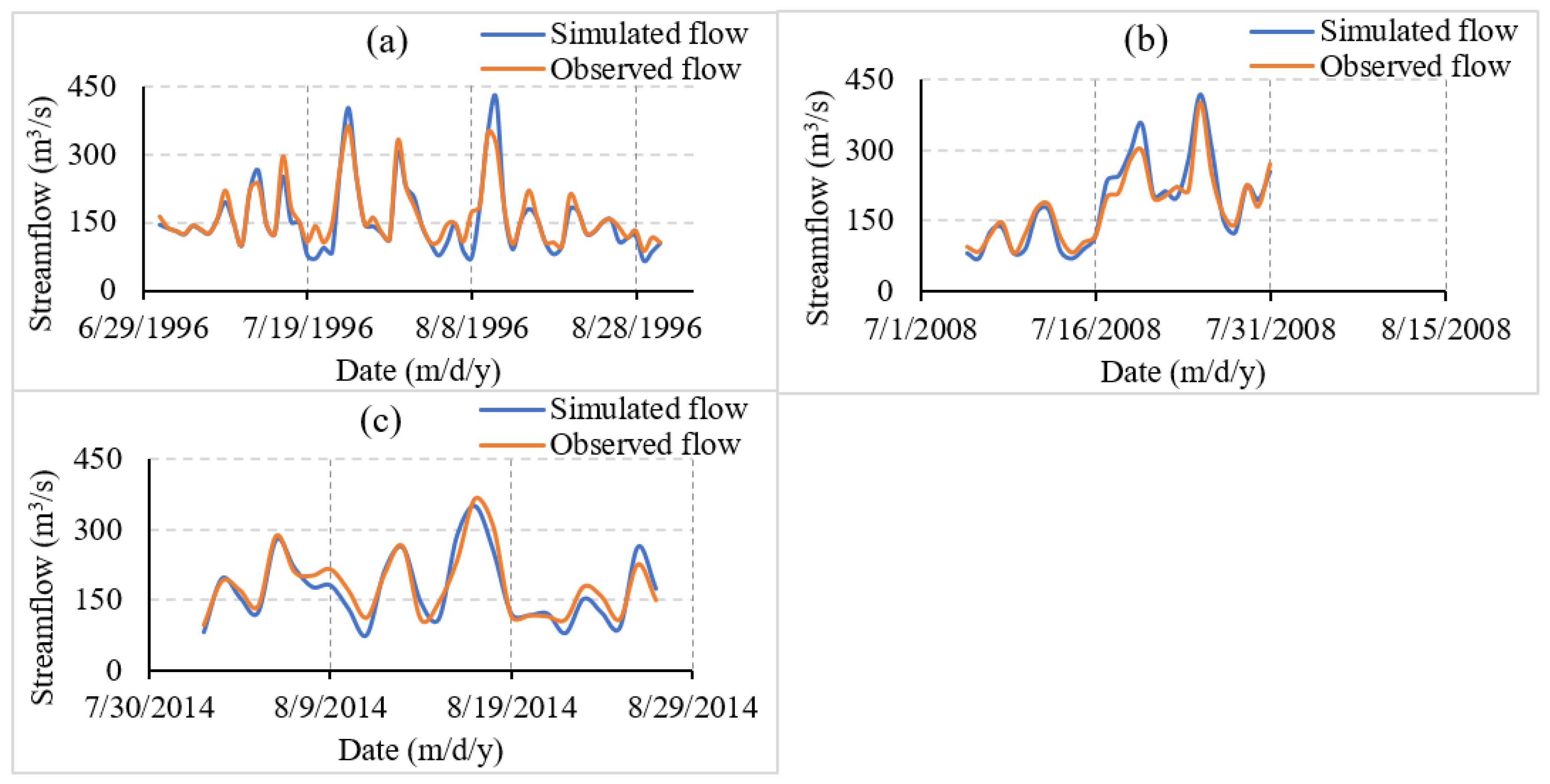
In this study, model calibration was performed for two selected events: Event-1, which occurred from July 1 to August 31, 1996, and Event-2, which occurred from July 5 to July 31, 2008. Model validation was conducted via Event-3, which occurred from August 2 to August 27, 2014. These events were specifically chosen to account for periods with high flood peaks.
2.9. Flood Source Area Identification (FSAI)
Flood source area identification (FSAI) is an important approach for identifying the main sources of downstream flooding. It helps rank subwatersheds on the basis of their contribution to peak flood magnitude at the main watershed outlet. In this study, FSAI was performed using the UFR, which was introduced by Saghafian & Khosroshahi [
35]. In the UFR approach, the contribution of each subwatershed can be computed as:
where is the gross flood index of the subwatershed in percent, is the outlet peak discharge in m3/s when all the subawtersheds are included in the base simulation, is the outlet peak discharge in m3/s when subawatersheds are excluded from the simulation, is the flood index of the subawtershed (m3/s/km2) based on the area of the subwatershed, and is the area of the subwatershed in km2.
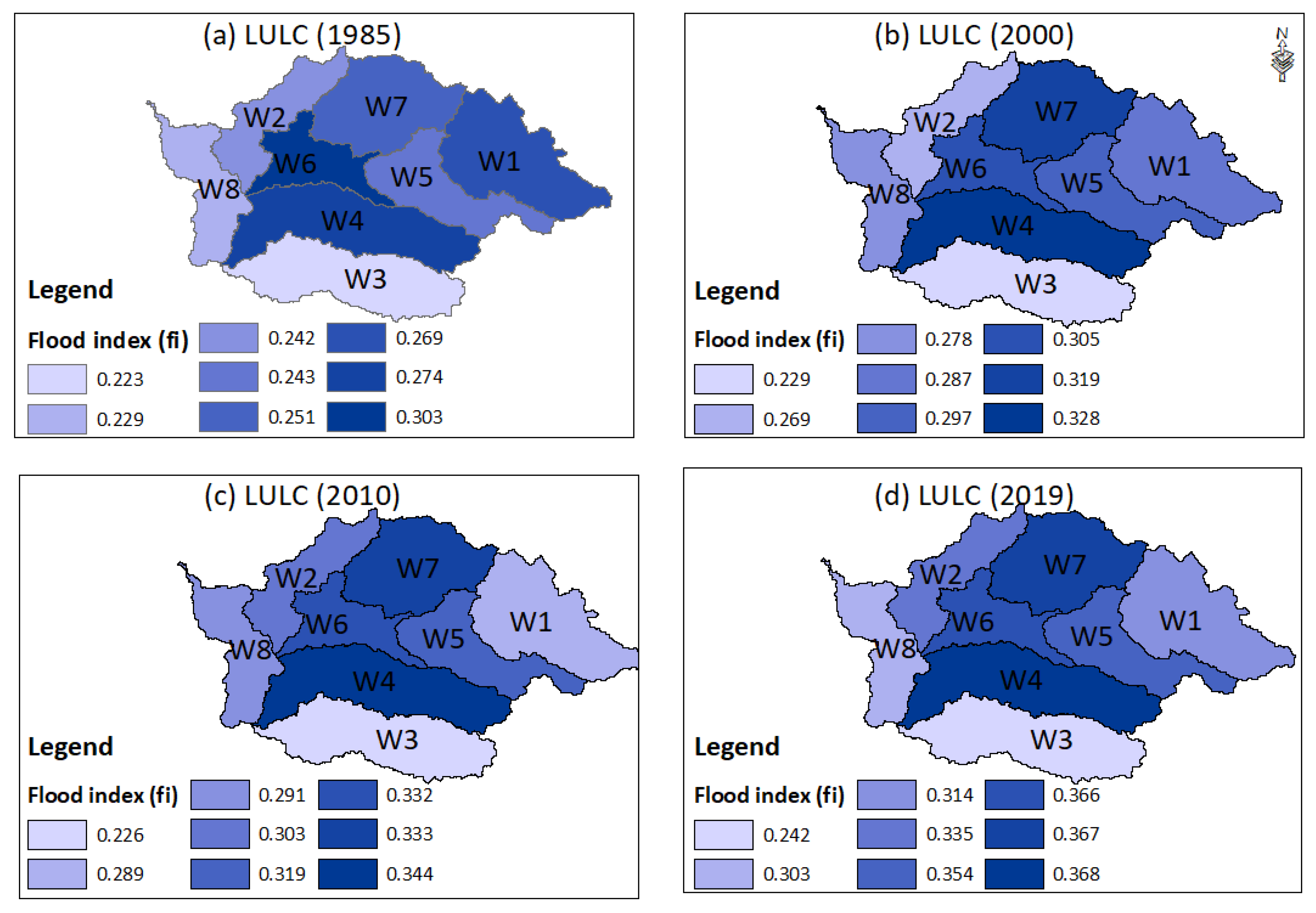
In the UFR approach, the subwatershed with the highest flood index value is ranked first (indicating the greatest contribution to peak discharge), whereas the subwatershed with the lowest flood index value is ranked last, indicating the least contribution. In this study, a calibrated HEC-HMS model incorporating all subwatershed components was first developed. The flood indices FI and fi for each subwatershed were subsequently calculated by disconnecting or eliminating a chosen subwatershed unit while maintaining the connections of the other subwatersheds. This process was repeated for all subwatersheds, allowing for a comprehensive analysis. In this regard, the analysis was also conducted under different conditions to investigate the impacts of LULC changes on the flood index values.
2.10. Combined Impacts of LULC and Climate Change on High Flows
The combined impacts of LULC and climate change on high flows, specifically on the annual maximum (AM) 1-day flows, were analyzed by simulating historical and future conditions using the calibrated HEC-HMS model, driven by AM 1-day rainfall. To assess these impacts on high flow extremes, flow duration curves (FDCs) were constructed from the AM flow series. The FDC construction process involved (1) sorting AM flows in descending order, (2) ranking the AM flows, (3) calculating the probability of exceedance for each flow value, and (4) plotting the AM flow series on the y-axis against the probability of exceedance on the x-axis. In this study, the probability of exceedance was calculated using the Weibull formula:
where is the probability of exceedance (%), m is the rank of the flow value, and N is the total number of flow data points.
5. Conclusions
This study assessed the impacts of LULC and climate changes on high flow extremes in the Gumara watershed using the HEC-HMS model. Merged rainfall data (1981–2019) and multi-model ensemble means from CMIP5 and CMIP6 models were utilized for historical (1981–2005), near-future (2031–2055), and far-future (2056–2080) periods, with future climate scenarios projected under RCP4.5, RCP8.5, SSP2-4.5, and SSP5-8.5 pathways. Historical LULC maps (1985, 2000, 2010, and 2019) and projected LULC scenarios (BAU-2035, BAU-2065, GOV-2035, and GOV-2065) were incorporated to analyze the effects of LULC change on flood risk.
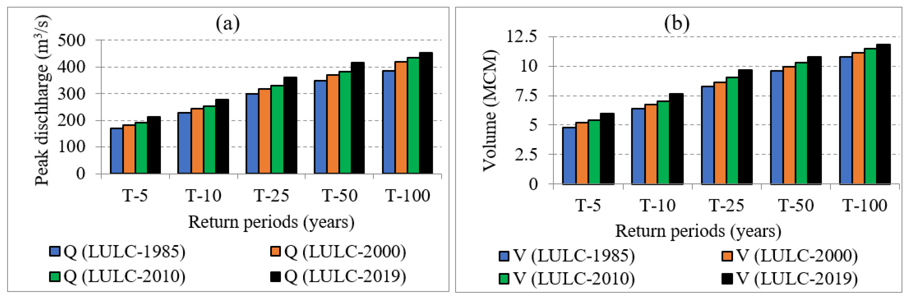
The long-term observation period (1981–2019) showed a significant increase in peak discharge under recent LULC conditions, with peak values rising by 24.9% for the 5-year return period and by 17.6% for the 100-year return period, indicating a decreasing influence of LULC changes with higher return periods. The flood source areas identified using the UFR approach revealed subwatersheds W4 and W6 as consistent contributors to high runoff across various LULC conditions, making them priority areas for flood mitigation efforts.
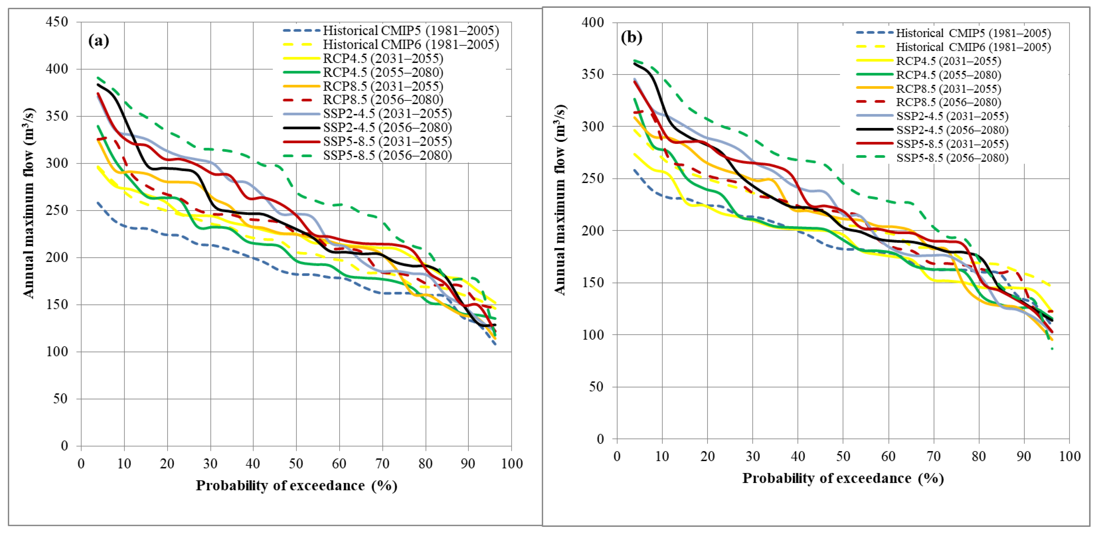
Future projections indicate a further increase in high flows, especially under the SSP5-8.5 (2056–2080) climate scenario combined with BAU-2065 land use, where flows are projected to increase by up to 20.5%, suggesting an increased flood risk in the region. In contrast, the GOV scenario, which promotes afforestation, shows a smaller flow increase of up to 9.0%, demonstrating that sustainable land management practices can help mitigate climate change impacts on extreme flows.
In summary, this study integrated RF-MERGE, GIS, and HEC-HMS models to investigate the effects of LULC and climate changes on high-flow extremes in the Gumara watershed. The findings provide valuable insights for watershed managers and land use planners to prioritize subwatersheds and develop effective flood risk management practices. The study suggests the coordinated participation of local governments, non-governmental organizations, basin initiatives, and communities to collaboratively mitigate the adverse effects of future flood events. Future research could expand on this work by using climate model ensembles based on MLEP approaches, integrating satellite-based soil moisture data, and conducting hydraulic flood modeling downstream of the Gumara watershed. These efforts would further inform flood mitigation strategies across the region.
Figure 1.
Location map of the study area. (a) Location map of the Upper Blue Nile (UBN) basin within the 12 river basins of Ethiopia; (b) Location map of the Gumara watershed within the Lake Tana subbasin; (c) Detailed map showing the rainfall and streamflow gauging stations, stream network, climate model grid (25 km x 25 km) and grid center for the NASA dataset, and elevation map of the upstream (flood source area) part of the Gumara watershed.
Figure 2.
(a) Elevation, (b) slope, (c) hydrologic soil groups (HSGs), and (d-k) historical and projected land use and land cover maps of the Gumara watershed for the historical (1985, 2000, 2010, and 2019) and future years (2035 and 2065) under the business as usual (BAU) and governance (GOV) scenarios.
Figure 3.
Methodological framework of the study. In the figure, boxes highlighted with grey color represent the main processing algorithm, tool, and hydrological model used in the study.
Figure 3.
Methodological framework of the study. In the figure, boxes highlighted with grey color represent the main processing algorithm, tool, and hydrological model used in the study.
Figure 4.
Observed ground-based rainfall and discharge data from 1981 to 2019 for the Gumara watershed. (a) Double mass curve analysis, (b) mean annual rainfall of each ground-based rainfall station, (c) mean monthly rainfall, and (d) mean monthly discharge.
Figure 4.
Observed ground-based rainfall and discharge data from 1981 to 2019 for the Gumara watershed. (a) Double mass curve analysis, (b) mean annual rainfall of each ground-based rainfall station, (c) mean monthly rainfall, and (d) mean monthly discharge.
Figure 5.
Comparison of cumulative distribution functions (CDFs) of daily observed rainfall data from RF-MERGE and historical CMIP5 and CMIP6 models for the period 1981–2005.
Figure 5.
Comparison of cumulative distribution functions (CDFs) of daily observed rainfall data from RF-MERGE and historical CMIP5 and CMIP6 models for the period 1981–2005.
Figure 6.
A 30-meter spatial resolution gridded runoff curve numbers for the historical years (a-d) and future scenarios (e-h). The gray shaded areas in the figure illustrate the gradient orientation of the runoff curve number, with maximum values along the north and south directions and minimum values in the middle of the watershed.
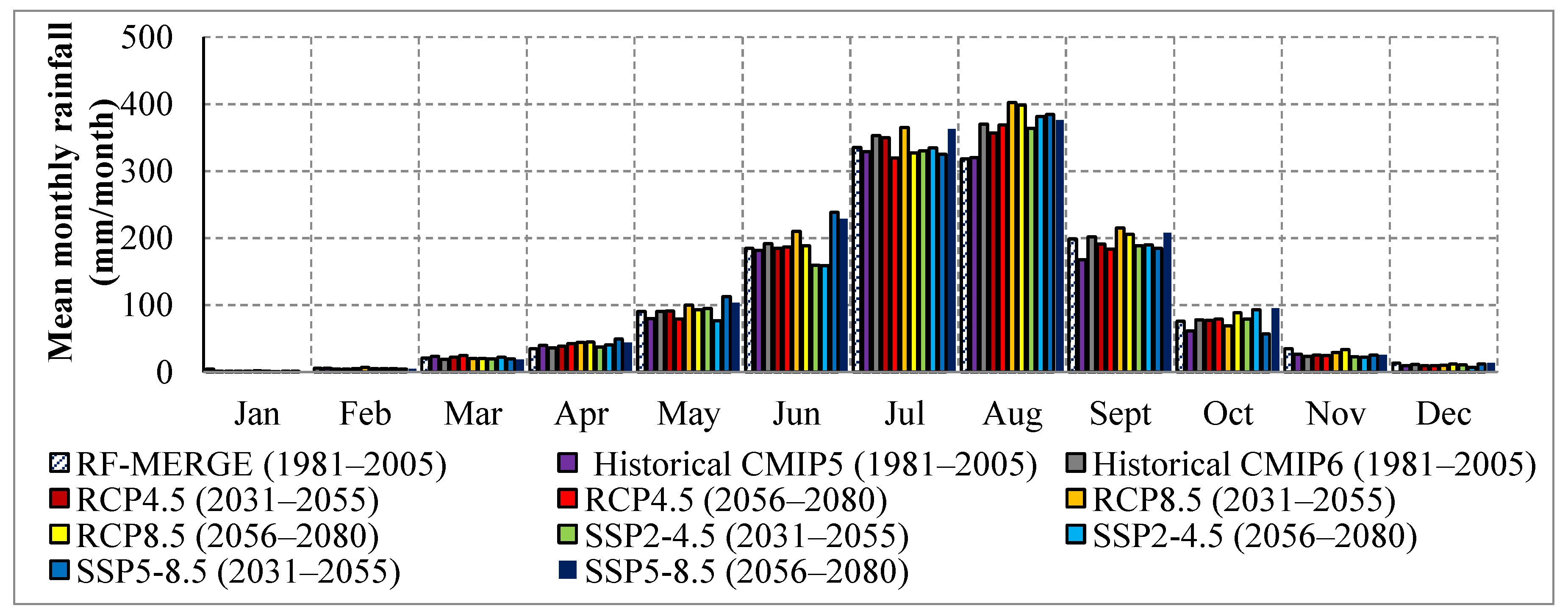
Figure 7.
Historical (1981–2005) and projected (2031–2080) mean monthly rainfall (mm/month) of the Gumara watershed, estimated from RF-MERGE data and multi-model ensemble means from CMIP5 and CMIP6.
Figure 7.
Historical (1981–2005) and projected (2031–2080) mean monthly rainfall (mm/month) of the Gumara watershed, estimated from RF-MERGE data and multi-model ensemble means from CMIP5 and CMIP6.
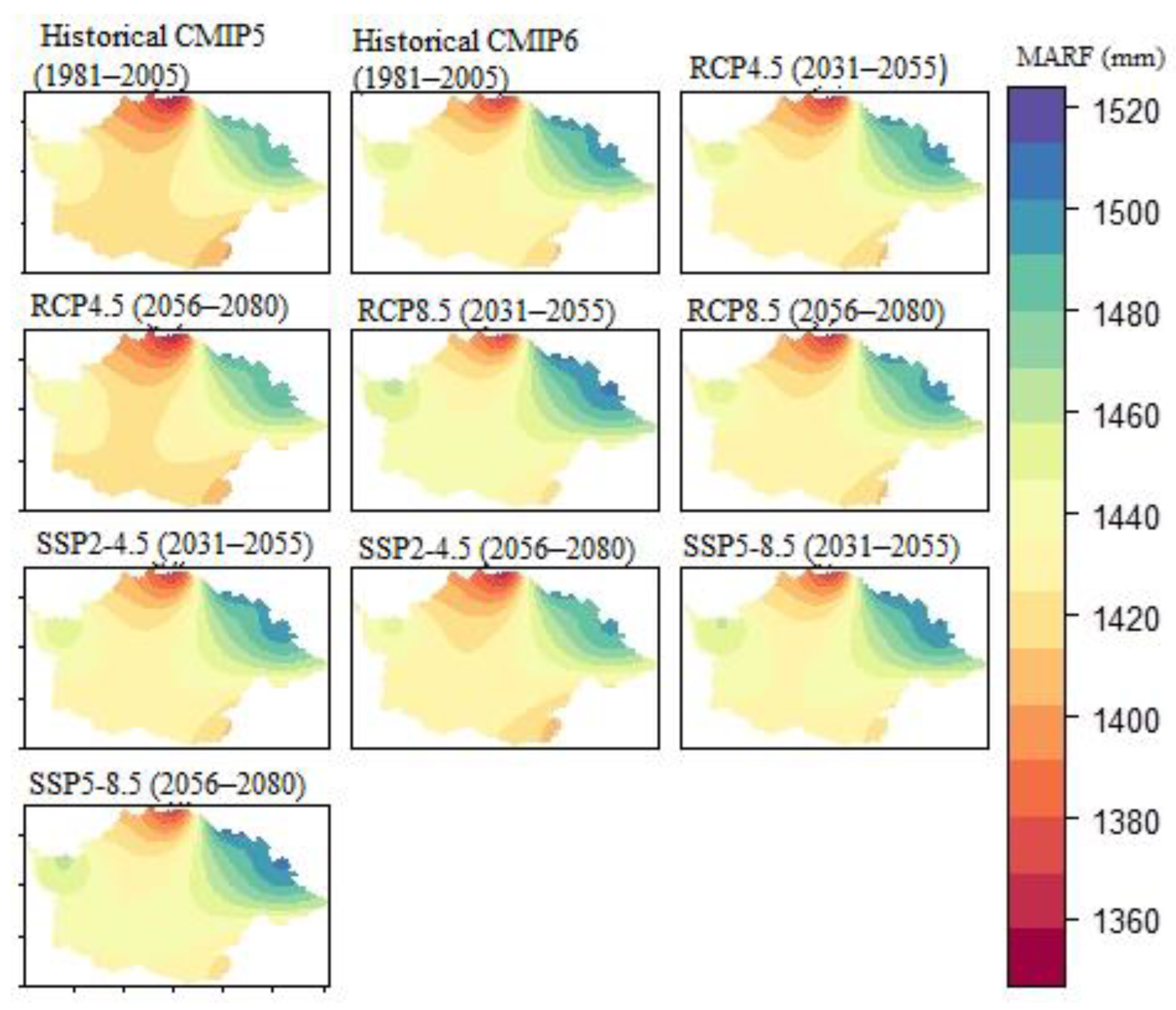
Figure 8.
Spatial distribution of mean annual rainfall (MARF) in the historical (1981-2005) and two future periods: near-future (2031-2056) and far-future (2056-2080) under different climate scenarios. In the figures, different color gradients show the distribution of rainfall in the study area, where the dark blue color grade shows areas that receive the highest mean annual rainfall.
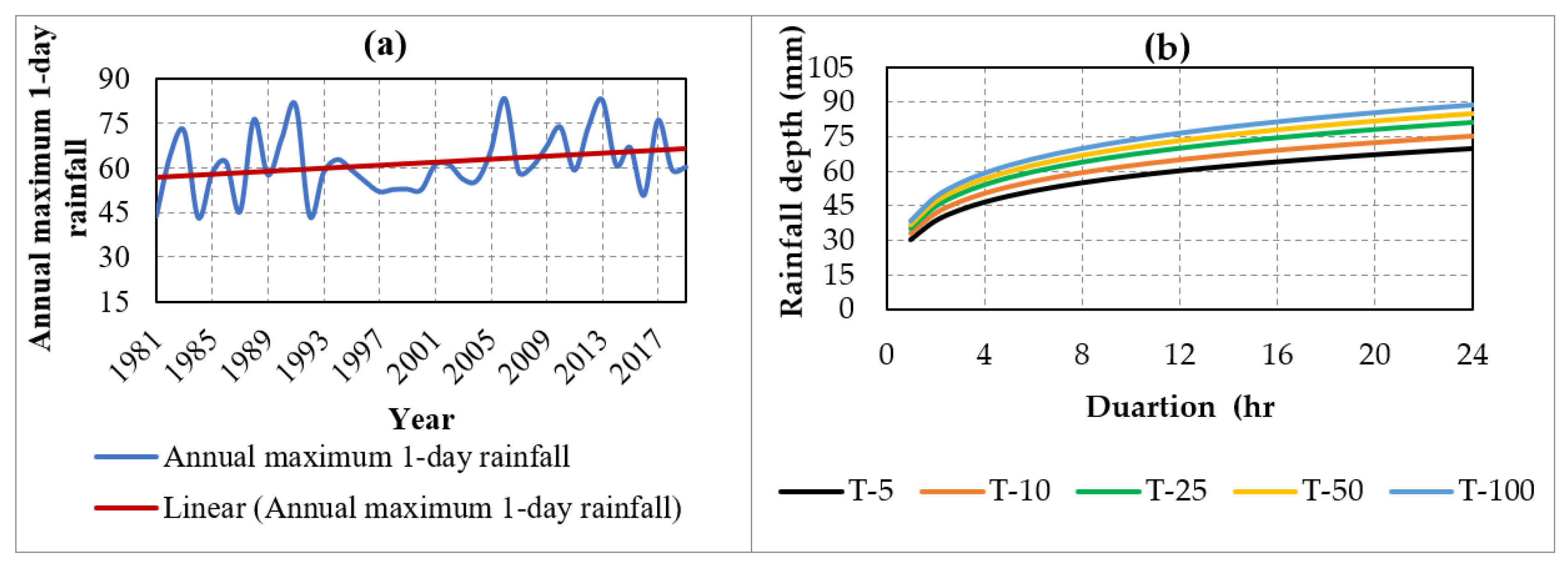
Figure 9.
(a) Temporal variation of the long-term annual maximum (AM) 1-day rainfall series from RF-MERGE estimates (1981–2019) and (b) depth-duration-frequency (DDF) curve developed from RF-MERGE rainfall. In panel (a), the red line illustrates the increasing linear trend of annual maximum 1-day rainfall.
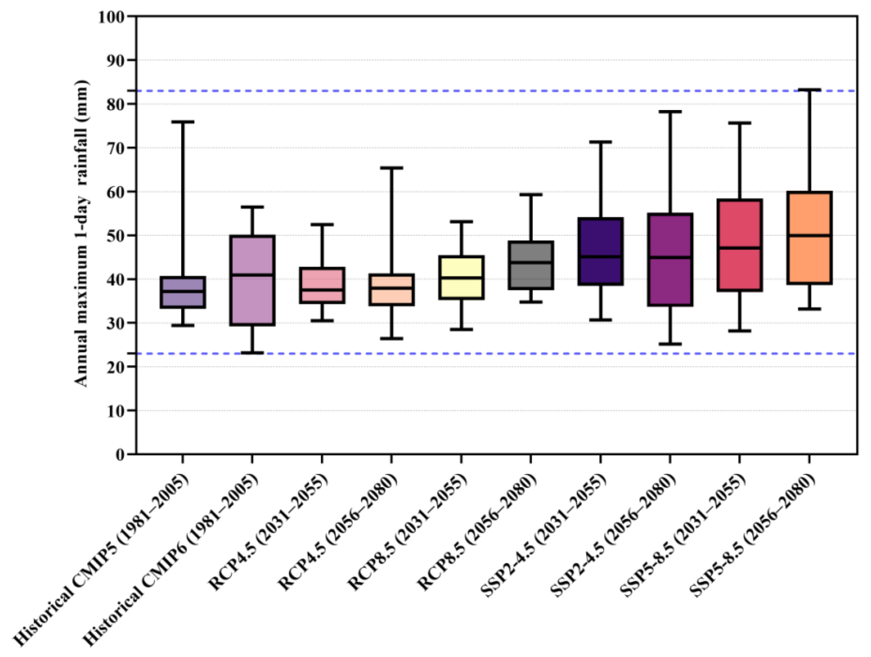
Figure 10.
Box plot of historical (1981–2005) and projected (2031–2080) annual maximum (AM) 1-day rainfall. The plot summarizes the minimum, first quartile (Q1), median, third quartile (Q3), and maximum values of the rainfall data. The blue dashed lines indicate the full range of data across the study periods.
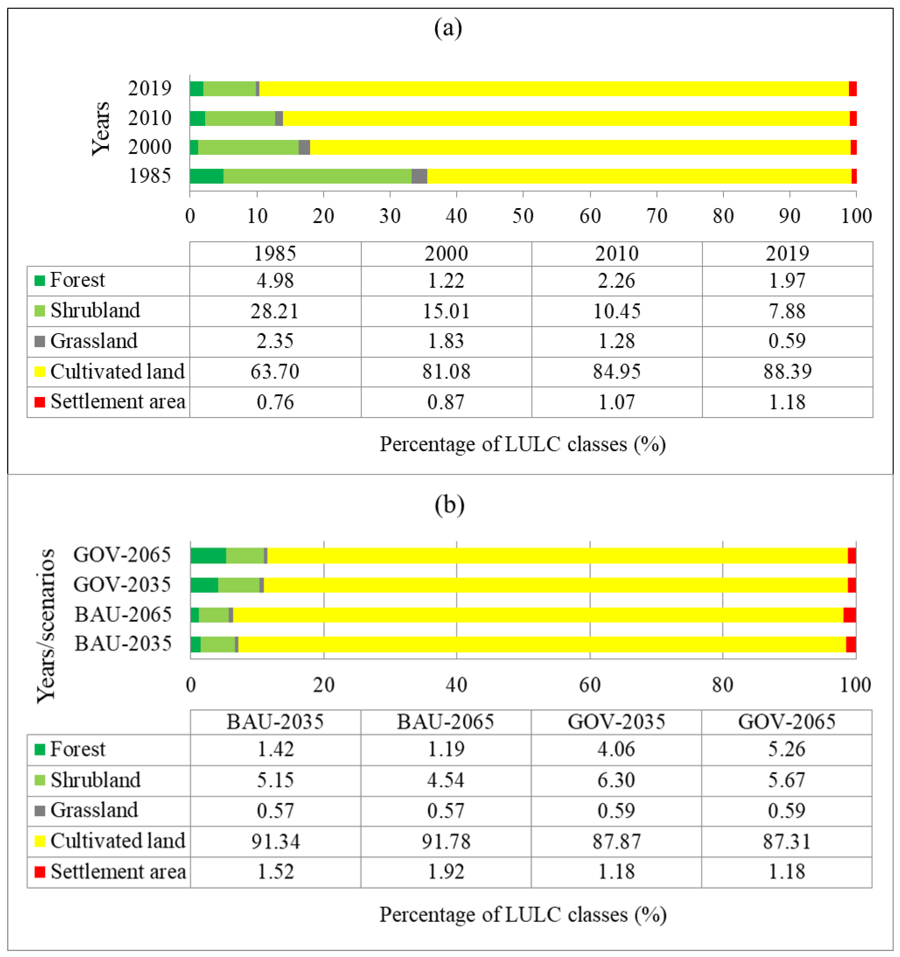
Figure 11.
Percentage coverage of land use and land cover (LULC) classes of the Gumara watershed. (a) Historical years (1985, 2000, 2010, and 2019) and (b) Future years (2035 and 2065) under the business as usual (BAU) and governance (GOV) scenarios.
Figure 11.
Percentage coverage of land use and land cover (LULC) classes of the Gumara watershed. (a) Historical years (1985, 2000, 2010, and 2019) and (b) Future years (2035 and 2065) under the business as usual (BAU) and governance (GOV) scenarios.
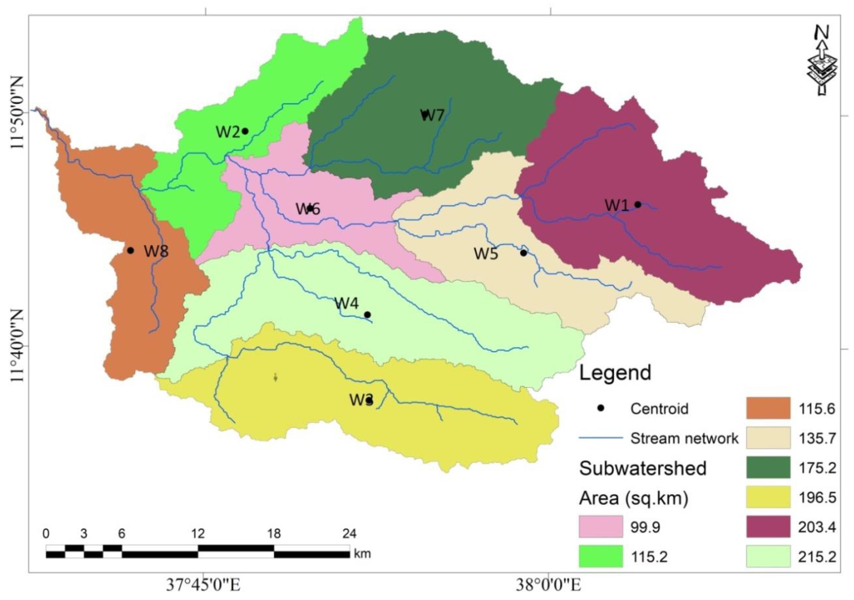
Figure 12.
Delineated subwatershed’s area, centroids, and stream network of the Gumara watershed as delineated in the HEC-HMS model.
Figure 12.
Delineated subwatershed’s area, centroids, and stream network of the Gumara watershed as delineated in the HEC-HMS model.
Figure 13.
Model sensitivity analysis for the runoff curve number (CN) from August 13 to August 31, 2010.
Figure 13.
Model sensitivity analysis for the runoff curve number (CN) from August 13 to August 31, 2010.
Figure 14.
Observed and simulated discharge for selected events: (a) Event-1 (calibration) from July 1 to August 31, 1996; (b) Event-2 (calibration) from July 5 to July 31, 2008; (c) Event-3 (validation), from August 2 to August 27, 2014.
Figure 14.
Observed and simulated discharge for selected events: (a) Event-1 (calibration) from July 1 to August 31, 1996; (b) Event-2 (calibration) from July 5 to July 31, 2008; (c) Event-3 (validation), from August 2 to August 27, 2014.
Figure 15.
(a) Comparison of simulated peak discharge (Q) under various land use conditions across different return periods, and (b) Comparison of simulated runoff volume (V) under various land use conditions across different return periods.
Figure 15.
(a) Comparison of simulated peak discharge (Q) under various land use conditions across different return periods, and (b) Comparison of simulated runoff volume (V) under various land use conditions across different return periods.
Figure 16.
Computed flood index () values estimated using the Unit Flood Response (UFR) approach for a 50-year return period peak discharge under different LULC conditions: (a) LULC-1985, (b) LULC-2000, (c) LULC-2010, and (d) LULC-2019. The blue color gradient represents flood index levels across subwatersheds, with the darkest blue indicating subwatersheds with the highest runoff potential.
Figure 17.
Comparison between historical and future annual maximum 1-day flow duration curves. (a) Future climate combined with the BAU land use scenario and (b) Future climate combined with the GOV land use scenario.
Figure 17.
Comparison between historical and future annual maximum 1-day flow duration curves. (a) Future climate combined with the BAU land use scenario and (b) Future climate combined with the GOV land use scenario.
Table 1.
Location and elevation information of the eight ground-based meteorological stations located in and around the Gumara watershed.
Table 1.
Location and elevation information of the eight ground-based meteorological stations located in and around the Gumara watershed.
| No. |
Station name |
Latitude (o) |
Longitude (o) |
Elevation (m) |
| 1 |
Amed Ber |
11.91 |
37.88 |
2051 |
| 2 |
Arb Gebeya |
11.62 |
37.74 |
2248 |
| 3 |
Debre Tabor |
11.87 |
38.01 |
2612 |
| 4 |
Gassay |
11.79 |
38.13 |
2789 |
| 5 |
Hamusit |
11.78 |
37.56 |
1954 |
| 6 |
Mekaneyesus |
11.58 |
37.90 |
2374 |
| 7 |
Wanzaye |
11.78 |
37.68 |
1821 |
| 8 |
Wereta |
11.92 |
37.70 |
1819 |
Table 2.
Details of the gridded rainfall products (GRFPs) used in the rainfall data merging process.
Table 2.
Details of the gridded rainfall products (GRFPs) used in the rainfall data merging process.
| Gridded rainfall product |
Spatial resolution (km) |
Source (access) |
Reference |
| MSWEP |
10 km × 10 km |
https://www.gloh2o.org/mswep |
[54] |
| CHIRPS |
5 km × 5 km |
https://chg.geog.ucsb.edu/data/chirps/ |
[55] |
| ERA5-Land |
10 km × 10 km |
https://www.ecmwf.int/en/forecasts/datasets/era5 |
[56] |
Table 3.
Descriptions of the NASA NEX-GDDP dataset (CMIP5 and CMIP6 climate models) used in this study.
Table 3.
Descriptions of the NASA NEX-GDDP dataset (CMIP5 and CMIP6 climate models) used in this study.
| GCM |
Name |
Spatial resolution (km) |
Modeling center |
Country |
| CMIP5 |
MIROC5 |
25 km x 25 km |
National Institute for Environmental Studies, the University of Tokyo |
Japan |
| MRI-CGCM3 |
25 km x 25 km |
Meteorological Research Institute |
Japan |
| CanESM2 |
25 km x 25 km |
Canadian Centre for Climate Modeling and Analysis |
Canada |
| MPI-ESM1-2-LR |
25 km x 25 km |
Max Planck Institute for Meteorology |
Germany |
| CMIP6 |
MPI-ESM1-2-LR |
25 km x 25 km |
Max Planck Institute for Meteorology |
Germany |
| MRI-ESM2-0 |
25 km x 25 km |
Meteorological Research Institute |
Japan |
| CNRM-CM6-1 |
25 km x 25 km |
Centre National de Recherches Meteorologiques |
France |
| BCC-CSM2-MR |
25 km x 25 km |
Beijing Climate Center, China Meteorological Administration |
China |
Table 4.
Characteristics of subwatersheds (area, slope, longest flow path length and slope, centroidal flow path length and slope, and drainage density).
Table 4.
Characteristics of subwatersheds (area, slope, longest flow path length and slope, centroidal flow path length and slope, and drainage density).
| Subwatershed |
Area (km2) |
Subwatershed slope (%) |
Longest flow path length (km) |
Longest flow path slope (%) |
Centroidal flow path length (km) |
Centroidal flow path slope (%) |
| W1 |
203.4 |
24.20 |
30.8 |
4.952 |
11.4 |
1.89 |
| W2 |
115.2 |
13.10 |
28.9 |
1.748 |
13.3 |
0.35 |
| W3 |
196.5 |
15.00 |
34.0 |
1.39 |
14.2 |
1.13 |
| W4 |
215.2 |
19.40 |
34.2 |
2.287 |
13.0 |
1.06 |
| W5 |
135.7 |
24.20 |
35.9 |
3.118 |
15.1 |
1.94 |
| W6 |
99.9 |
14.50 |
25.8 |
1.871 |
10.3 |
0.18 |
| W7 |
175.2 |
19.70 |
27.2 |
2.936 |
10.0 |
1.10 |
| W8 |
115.6 |
15.40 |
33.6 |
1.999 |
21.0 |
0.97 |
| Gumara |
1256.7 |
|
|
|
|
|
Table 5.
Changes in peak discharge due to changes in the runoff curve number (CN) with for selected events (from August 13 to August 31, 2010).
Table 5.
Changes in peak discharge due to changes in the runoff curve number (CN) with for selected events (from August 13 to August 31, 2010).
| Simulation |
Peak discharge (m3/s) |
Change in peak discharge (%) |
| Initial simulation |
280 |
– |
| CN (+25%) |
307.4 |
9.79 |
| CN (-25%) |
244.4 |
-12.71 |
Table 6.
Model performance evaluation during calibration and validation.
Table 6.
Model performance evaluation during calibration and validation.
| Event |
Peak discharge (m3/s) |
|
Performance evaluation |
| Observed |
Simulated |
|
RMSE (m3/s) |
R |
NSE |
PBIAS |
| Event 1 (calibration) |
362 |
423.6 |
|
27.1 |
0.89 |
0.82 |
-5.19 |
| Event 2 (calibration) |
402 |
417.7 |
|
25.69 |
0.94 |
0.88 |
1.95 |
| Event 3 (validation) |
365.5 |
350.8 |
|
26.70 |
0.87 |
0.85 |
-3.99 |
Table 7.
Calibrated model parameter values for the runoff volume, direct runoff, and routing models.
Table 7.
Calibrated model parameter values for the runoff volume, direct runoff, and routing models.
| Runoff volume model: SCS-Curve Number |
|
Direct runoff model: SCS-unit hydrograph |
|
Routing model: Muskingum model |
| Subwatershed |
Initial abstraction (mm) |
Curve number |
|
Subwatershed |
Lag time (min.) |
|
Reach |
Muskingum K (hr.) |
Muskingum X (hr.) |
| W1 |
15.2 |
77 |
|
W1 |
106 |
|
R1 |
1 |
0.45 |
| W2 |
14.9 |
77 |
|
W2 |
150 |
|
R2 |
0.76 |
0.50 |
| W3 |
14.3 |
78 |
|
W3 |
186 |
|
R3 |
0.15 |
0.35 |
| W4 |
14.3 |
78 |
|
W4 |
155 |
|
R4 |
0.1 |
0.30 |
| W5 |
14.9 |
77 |
|
W5 |
142 |
|
R5 |
0.58 |
0.50 |
| W6 |
15.5 |
77 |
|
W6 |
134 |
|
R6 |
1.1 |
0.50 |
| W7 |
15.2 |
77 |
|
W7 |
118 |
|
R7 |
1.17 |
0.45 |
| W8 |
14.3 |
78 |
|
W8 |
160 |
|
R8 |
0.36 |
0.40 |
Table 8.
Changes in peak discharge and runoff volume for different return periods between LULC-1985 and LULC-2019.
Table 8.
Changes in peak discharge and runoff volume for different return periods between LULC-1985 and LULC-2019.
| Return period |
Peak discharge (m3/s) |
Runoff volume (MCM) |
| 1985 |
2019 |
Change (%) |
1985 |
2019 |
Change (%) |
| T-5 |
169.4 |
211.7 |
24.9 |
4.8 |
5.96 |
24.2 |
| T-10 |
228.4 |
278.5 |
21.9 |
6.4 |
7.66 |
19.7 |
| T-25 |
298.9 |
359.5 |
20.2 |
8.3 |
9.66 |
16.4 |
| T-50 |
348.4 |
416.7 |
19.6 |
9.6 |
10.8 |
12.5 |
| T-100 |
384.8 |
452.7 |
17.6 |
10.8 |
11.8 |
9.3 |
Table 9.
Comparison of 50-year peak discharge generation in the Gumara watershed under different land use conditions.
Table 9.
Comparison of 50-year peak discharge generation in the Gumara watershed under different land use conditions.
| Subwatershed |
Area (km2) |
(m3/s) |
(m3/s) |
|
|
(m3/s//km2) |
|
| LULC-1985 |
|
|
|
|
|
| W1 |
203.4 |
74.9 |
270.7 |
16.8 |
2 |
0.269 |
3 |
| W2 |
115.2 |
37.5 |
297.5 |
8.6 |
7 |
0.242 |
6 |
| W3 |
196.5 |
65.6 |
281.5 |
13.5 |
4 |
0.223 |
8 |
| W4 |
215.2 |
67 |
266.5 |
18.1 |
1 |
0.274 |
2 |
| W5 |
135.7 |
40.1 |
292.4 |
10.1 |
5 |
0.243 |
5 |
| W6 |
99.9 |
42 |
295.1 |
9.3 |
6 |
0.303 |
1 |
| W7 |
175.2 |
55.7 |
281.4 |
13.5 |
3 |
0.251 |
4 |
| W8 |
115.6 |
40.6 |
298.9 |
8.1 |
8 |
0.229 |
7 |
| Gumara |
1256.7 |
325.4 |
|
|
|
|
|
| LULC-2000 |
|
|
|
|
|
| W1 |
203.4 |
81.8 |
310.8 |
15.8 |
2 |
0.287 |
5 |
| W2 |
115.2 |
40.5 |
338.1 |
8.4 |
7 |
0.269 |
7 |
| W3 |
196.5 |
69.6 |
324.1 |
12.2 |
4 |
0.229 |
8 |
| W4 |
215.2 |
80.6 |
298.5 |
19.1 |
1 |
0.328 |
1 |
| W5 |
135.7 |
50.8 |
328.8 |
10.9 |
5 |
0.297 |
4 |
| W6 |
99.9 |
39.9 |
338.6 |
8.3 |
8 |
0.305 |
3 |
| W7 |
175.2 |
73.4 |
313.2 |
15.1 |
3 |
0.319 |
2 |
| W8 |
115.6 |
50.2 |
337 |
8.7 |
6 |
0.278 |
6 |
| Gumara |
1256.7 |
369.1 |
|
|
|
|
|
| LULC-2010 |
|
|
|
|
|
| W1 |
203.4 |
82.6 |
324.8 |
15.3 |
2 |
0.289 |
7 |
| W2 |
115.2 |
45.5 |
348.7 |
9.1 |
6 |
0.303 |
5 |
| W3 |
196.5 |
70.3 |
339.1 |
11.6 |
4 |
0.226 |
8 |
| W4 |
215.2 |
84.6 |
309.6 |
19.3 |
1 |
0.344 |
1 |
| W5 |
135.7 |
54.8 |
340.3 |
11.3 |
5 |
0.319 |
4 |
| W6 |
99.9 |
42.9 |
350.4 |
8.7 |
8 |
0.332 |
3 |
| W7 |
175.2 |
75.4 |
325.5 |
15.1 |
3 |
0.333 |
2 |
| W8 |
115.6 |
51.1 |
350 |
8.8 |
7 |
0.291 |
6 |
| Gumara |
1256.7 |
383.6 |
|
|
|
|
|
| LULC-2019 |
|
|
|
|
|
| W1 |
203.4 |
89.7 |
352.8 |
15.3 |
3 |
0.314 |
6 |
| W2 |
115.2 |
51.4 |
378.1 |
9.3 |
6 |
0.335 |
5 |
| W3 |
196.5 |
76.6 |
369.1 |
11.4 |
5 |
0.242 |
8 |
| W4 |
215.2 |
90.7 |
337.5 |
19.0 |
1 |
0.368 |
1 |
| W5 |
135.7 |
61.1 |
368.6 |
11.5 |
4 |
0.354 |
4 |
| W6 |
99.9 |
48.3 |
380.1 |
8.8 |
7 |
0.366 |
3 |
| W7 |
175.2 |
83.4 |
352.3 |
15.5 |
2 |
0.367 |
2 |
| W8 |
115.6 |
53 |
381.7 |
8.4 |
8 |
0.303 |
7 |
| Gumara |
1256.7 |
416.7 |
|
|
|
|
|
Table 10.
Change in high flow of the Gumara watersheds under combined climate (RCP and SSP) and land use (BAU-2035, BAU-2065, GOV-2035, and GOV 2065) scenarios.
Table 10.
Change in high flow of the Gumara watersheds under combined climate (RCP and SSP) and land use (BAU-2035, BAU-2065, GOV-2035, and GOV 2065) scenarios.
| Scenario/period |
|
Flow under combined future climate and BAU land use scenario |
|
Flow under combined future climate and GOV land use scenario |
| BAU land use scenario |
Mean annual maximum flow (m3/s) |
Change (%) |
GOV land use scenario |
Mean annual maximum flow (m3/s) |
Change (%) |
| Historical CMIP5 (1981–2005) |
|
188.1 |
– |
|
188.1 |
– |
| Historical CMIP6 (1981–2005) |
|
211.5 |
– |
|
211.5 |
– |
| RCP4.5 (2031–2055) |
2035 |
224 |
19.1 |
2035 |
200.5 |
6.6 |
| RCP4.5 (2056–2080) |
2065 |
209.4 |
11.3 |
2065 |
200.2 |
6.4 |
| RCP8.5 (2031–2055) |
2035 |
223.5 |
18.9 |
2035 |
204.0 |
8.5 |
| RCP8.5 (2056–2080) |
2065 |
225.7 |
20.0 |
2065 |
202.8 |
7.8 |
| SSP2-4.5 (2031–2055) |
2035 |
243.1 |
14.9 |
2035 |
225.1 |
6.4 |
| SSP2-4.5 (2056–2080) |
2065 |
237.4 |
12.3 |
2065 |
223.9 |
5.9 |
| SSP5-8.5 (2031–2055) |
2035 |
246.4 |
16.5 |
2035 |
226.4 |
7.0 |
| SSP5-8.5 (2056–2080) |
2065 |
254.8 |
20.5 |
2065 |
230.6 |
9.0 |
Table 11.
The mean annual maximum flow (Q) of the Gumara watershed, in m³/s, across different probability of exceedance ranges, as estimated under combined climate and land use scenarios.
Table 11.
The mean annual maximum flow (Q) of the Gumara watershed, in m³/s, across different probability of exceedance ranges, as estimated under combined climate and land use scenarios.
| Scenario/period |
|
Flow under combined future climate and BAU land use scenario |
|
Flow under combined future climate and GOV land use scenario |
| BAU land use scenario |
Q0–Q25
|
Q26–Q50
|
Q51–Q75
|
Q76–Q100
|
GOV land use scenario |
Q0–Q25
|
Q26–Q50
|
Q51–Q75
|
Q76–Q100
|
| Historical CMIP5 (1981-2005) |
_ |
234.7 |
200.4 |
172.3 |
142.8 |
_ |
234.7 |
200.4 |
172.3 |
142.8 |
| Historical CMIP6 (1981-2005) |
_ |
265.5 |
224.9 |
191.6 |
161.7 |
_ |
265.5 |
224.9 |
191.6 |
161.7 |
| RCP4.5 (2031–2055) |
2035 |
269.6 |
234.4 |
212.9 |
177.5 |
2035 |
242.4 |
203.5 |
168.4 |
141.7 |
| RCP4.5 (2055–2080) |
2065 |
285.7 |
219.5 |
182.9 |
147.8 |
2065 |
268.4 |
203.8 |
172.1 |
132.3 |
| RCP8.5 (2031–2055) |
2035 |
293.2 |
244.6 |
209.3 |
143.4 |
2035 |
282.7 |
231 |
197 |
123.6 |
| RCP8.5 (2056–2080) |
2065 |
291 |
241 |
203.3 |
165.1 |
2065 |
276.7 |
227.9 |
184.4 |
149.3 |
| SSP2-4.5 (2031–2055) |
2035 |
330.8 |
274.9 |
206.3 |
155.2 |
2035 |
308 |
247.8 |
186 |
132.1 |
| SSP2-4.5 (2056–2080) |
2065 |
328.7 |
250.5 |
206.3 |
162.1 |
2065 |
310.7 |
227.4 |
189.2 |
144.8 |
| SSP5-8.5 (2031–2055) |
2035 |
327 |
272 |
218.1 |
164.3 |
2035 |
298.3 |
245.1 |
196.9 |
139.3 |
| SSP5-8.5 (2056–2080) |
2065 |
356.4 |
302.2 |
247.2 |
177.8 |
2065 |
331.6 |
271.5 |
219.7 |
143.5 |