
Submitted:
30 December 2025
Posted:
01 January 2026
You are already at the latest version
Preprints on COVID-19 and SARS-CoV-2
Abstract
India, a major emerging economy has historically been deeply affected by global economic shocks.
Understanding how its key economic factors such as Index of industrial production, wholesale prices, exchange rates and oil prices respond to these events is crucial for the nation's stability. This research aims to analyse India's macroeconomic responses to these three significant global shocks such as Financial crises 2008, recurring oil price shocks and Covid-19 pandemic.
Using monthly data from 1993 to 2024, this study employs co-integration tests for long-term linkages and a VECM for short-term dynamics (including IRF and FEVD). Quantile regression uncovers asymmetric crisis effects, whereas ARCH–GARCH models are employed to assess volatility persistence. The findings show long-term equilibrium linkages with significant error-correction. Further, oil price shocks affect inflation and industrial output through exchange rate adjustments. Quantile regression reveals intensified asymmetric effects at distribution extremes whereas Volatility analysis confirms clustering, with structural breaks identified during the Global Financial Crisis and COVID-19. It can be concluded that India's macroeconomic system is externally vulnerable but demonstrates partial resilience. Policy recommendations from this study includes building strategic oil reserves, adopting currency-oil hedging and enhancing overall crisis preparedness so as to achieve macroeconomic stability.
Keywords:
financial crises
; COVID‐19
; macroeconomic variables
; volatility
; oil price shocks
1. Introduction
India is among the fastest-growing economy across the globe and aims to achieve middle-income status by 2047 (Anant, 2015 ;Shanmugam & Odasseril, 2024).
As an Asian power, India has committed to achieving net-zero emissions by 2070 (World Bank, 2024). Economic health of any economy is assessed by the performance of its macroeconomic variables, with governments and policymakers striving to maintain this stability (Magbondé & Konté, 2022; Bhardwaj et al., 2023) but as witnessed by global disruptions in recent past in form of Covid-19, Global crises of 2008 or oil price shocks have had significant effect on performance and functioning of global economies.
These global events have influenced macroeconomic variables such as inflation, money supply, the Index of Industrial Production (IIP), foreign direct investment (FDI) and interest rates (Bhat et al., 2017).
The literature identifies macroeconomic indicators as crucial for achieving overall stability and evaluating economic functioning (Abbass et al., 2022). Present study investigates the effects of the 2008 financial crisis, the COVID-19 lockdowns, and oil prices on key economic indicators of India.
1.1. The Shock of 2008: A Macroeconomic Perspective
Increased bilateral trade and the formation of regional blocs have facilitated technological advancement while also introducing opportunities for volatility spillovers. During the 2008 financial crisis, the collapse of global financial institutions led to diminished cross-border trade, decreased industrial demand and elevated inflation rates (Bems, 2012; Federal Reserve, 2009). Specifically, India's GDP growth and industrial output declined by 3.1% and 2.4%, respectively and economy saw inflation exceeding 8% due to rising oil prices which was followed by significant depreciation of rupee (Singh, 2009; SBI's ECOWRAP, 2018). The economy underwent substantial macroeconomic adjustments in response to external shocks due to stimulus measures the central government deficit rose to 6% of GDP (Gupta, 2009; Bajpai, 2011).
On monetary policy front the Reserve Bank of India reduced the repo rate from 9% to 4.7% by April 2009, maintaining a CRR of 5% and an SLR of 24% to enhance liquidity (Islam & Rajan, 2009; Kumar & Vashisht, 2009; Amutha, 2013).
According to Economic Survey (2008-2009) merchandise exports amounted to US$168.7 billion in 2008–09, reflecting a 3.6% year-on-year growth, while imports increased by 14.3% to US$287.8 billion, thereby exacerbating trade imbalances. These developments illustrate that India’s macroeconomic indicators were sensitive and responsive to global disruptions. Table 1 below presents the performance of macroeconomic indicators during the financial crisis.
As evident from Table 1 while GDP growth was moderate and satisfactory, the industrial sector experienced a significant decline, with growth slowing to about 2.4% and inflation rising to 8.4%. The depreciation of the rupee further exacerbated the external balance and increased import costs. As shown in Figure 1, the GDP growth rate fell to roughly 2.4% during the 2008-2009 period.
These disruptions show how external shocks could destabilise India's industrial production, inflation and currency, revealing the economy's exposure to global volatility. Further, oil price movements have emerged as critical transmission channels of volatility (Petroleum Planning & Analysis Cell, 2025; Kundu et al., 2025). Given India's dependence on imported crude oil, fluctuations in the global oil markets have had an affect over inflation, exchange rates and growth of the economy. Hence making it imperative to throughly explore their macroeconomic implications (Deheri & Sahu, 2023; Sreenu, 2018).
1.2. Oil-Macroeconomy Relationship
For developing countries, Crude oil prices are pivotal to economic activities, serving as essential components for economic development (Ahmad et al. 2022; Alawadhi and Longe, 2024). Variations in these prices are largely influenced by structural shifts in supply, leading to either deficit or surplus (Brini et al. 2016). India, a major oil importer, is significantly dependent on imports for its industrial sectors. Oil price shocks have uneven impacts on economies and there macroeconomic variables such as inflation, exchange rate, unemployment, this is particularly evident for those economies who are major importers of oil (Zulfigarov and Neuenkirch, 2020), meaning where price increase tend to dampen output, while price decreases do not necessarily boost growth. Hamilton (1983, 2003) indicates that oil-importing economies frequently experience weak macroeconomic performance and financial instability. Tiwari et al. (2022), Sharma and Shrivastava (2021) illustrate that rising oil prices impact the macroeconomic stability of both developing and developed nations. In 2008, Brent crude oil reached a peak of USD 147 per barrel in July, contributing to India's current account deficit, which rose to 11% of GDP. In contrast, during the COVID-19 pandemic, prices dropped to USD 20 per barrel in April 2020, which helped lower inflation and ease the current account deficit (IMF, Livemint 2008).
These contrasting trends are evident in Figure 2.
Figure 2 depicts notable fluctuations in Brent crude oil prices from 2000 to 2024. As observed Prices notably surged before the 2008 financial crisis and then sharply declined during crises period (2008-2009) , followed by huge dip in 2020 due to COVID-19 pandemic. Recently, prices have stabilised between USD 70 and 90 per barrel, highlighting ongoing global economic uncertainty. It is crucial for policymakers to bolster the resilience of economies, especially emerging ones, against oil shocks (Antonakakis et al., 2017a; Hailemariam et al., 2019; Hajebi et al., 2022).
1.3. COVID-19 and Macro-Economic Fluctuations
Indian economy, recognised as one of the world's fastest-growing economy, encountered significant challenges during the COVID-19 pandemic in 2020, affecting every sector (Khalid, 2021). The pandemic essentially brought the entire economy to a halt (Jawad and Naz, 2023; Jawad et al., 2021), causing disruptions in trade, industry, tourism and agriculture (Yulfiswandi and Nopry, 2023). Beyond the health implications, the pandemic had serious implications for macroeconomic fundamentals (Daud et al., 2024; Denano, 2023). According to the Economics Observatory, India's GDP contracted by 24.4% from April to June 2020 due to nationwide lockdowns whereas National income figures for 2021-2022 indicated a 7.4% contraction in the second quarter (July-September 2020). Although there was a modest recovery in subsequent quarters, with GDP increasing by 0.5% and 1.6%, the overall decline for 2020-2021 was -7.3%. The second wave in 2021 further affected key macroeconomic indicators, including oil prices and exchange rates (Bama, 2022) prolonged lockdowns further influenced inflation, unemployment rates and GDP rates (Cho et al., 2025). In response to these crises, the government launched the "Atmanirbhar Bharat" program, introducing a ₹20 lakh crore stimulus package, equivalent to 10% of GDP, to stimulate demand and support sectors like MSMEs, agriculture and vulnerable populations (Ministry of Finance, 2020). Hence reviving the economy. Figure 3 below demonstrates downswing of Indian economy during crises.
As depicted in above figure 3, India experienced a notably severe economic contraction during the COVID-19 pandemic, a downturn more pronounced than that observed in many other nations
This challenging period highlighted India's inherent structural vulnerabilities, which render the economy susceptible to various global disruptions, including currency depreciation, trade imbalances, inflationary pressures and supply chain bottlenecks (IMF, 2025; World Bank, 2024; Eichengreen & Gupta, 2024). Consequently, key macroeconomic indicators such as the Index of Industrial Production, wholesale price inflation and exchange rates become crucial barometers of economic health (Chauhan, 2025). Analysing these indicators is vital for formulating effective policy strategies.
Motivated by recent disruptions in the global economy and their potential effects on emerging markets such as India, this study sets two core objectives:
- To analyse the asymmetric and volatility-related responses of India's key macroeconomic indicators (industrial production, inflation, and exchange rate) to major global disruptions: the 2008 global financial crisis, the COVID-19 pandemic and persistent oil price shocks.
- To develop and substantiate evidence-based policy frameworks that enhance India's macroeconomic resilience and strategic preparedness against future global disruptions.
2. Research Questions
- 3.
- Do oil price shocks, the global financial crisis, and the COVID-19 pandemic have differential impact on India’s macroeconomic indicators (IIP, WPI, exchange rate)?
- 4.
- Did oil price fluctuations contribute to inflation and industrial volatility in India?
- 5.
- Did oil price shocks, the global financial crisis and the COVID-19 had any short term and long term effects on India’s selected macroeconomic factors.
3. Methodology
3.1. Data
The present study employs monthly data spanning from 1993 to 2024, an extensive period that captures the ripple effects of three major global shocks: the 2008 financial crisis, the COVID-19 outbreak and recent oil price fluctuations. This timeline allows us to track how India’s macroeconomic structure responded across different phases of volatility.
The study focuses on four key macroeconomic indicators:
- Index of Industrial Production (IIP): A proxy for industrial performance and overall economic activity.
- Wholesale Price Index (WPI): Represents inflationary trends and cost pressures in the economy.
- Exchange Rate (USD/INR): Captures external sector sensitivity and currency volatility.
- International Crude Oil Prices (Brent): Serves as the external shock variable, given India's dependence on oil imports
3.2. Data and Variable Construction
The analysis utilises monthly data for India's key macroeconomic indicators, such as the Index of Industrial Production (IIP), Wholesale Price Index (WPI), nominal exchange rate (INR/USD) and Brent crude oil prices (US$/barrel). Historical series are updated to the latest base year. The IIP and WPI were adjusted seasonally using the X-13ARIMA-SEATS procedure. All series were converted into natural logarithms. This results in:
- Industrial growth: Δlog(IIP)
- Inflation: Δlog(WPI)
- Oil returns: Δlog(Brent)
- Exchange-rate depreciation: Δlog(INR/USD)
For robustness, oil prices are expressed in rupee terms as a log (Brent × INR/USD) to account for the effects of oil prices and exchange rates on the domestic economy.
3.3. Data Cleaning and Crisis Controls
Because extensive data have been employed, missing values are handled conservatively. When the gaps are short (two months or less), we interpolate linearly, and longer gaps are dropped. We also retain raw crisis observations, but conduct robustness checks in which (i) returns are winsorized at the 1% tails and (ii) the most extreme crisis months (e.g., April 2020 during the nationwide lockdown) are excluded. These checks confirmed that the results were not driven by a single outlier.
3.4. Pre-Testing and Structural Breaks
We employed ADF and KPSS unit root tests to determine the integration order of data properties. A Structural break analysis was conducted using the Zivot-Andrews tests for single breaks and Bai-Perron tests for multiple breaks, with break dates evaluated against the timelines of the Global Financial Crises and COVID-19. Gregory-Hansen tests are utilised as a robustness check for co-integration in the presence of structural breaks.
3.5. Crisis Coding and Robustness
Crisis dummies for the Global Financial Crises and COVID-19 are included as exogenous regressors in the sensitivity checks, although the main analysis relies on the structural identification of oil shocks and formal break tests.
3.6. Sources of Data Collection
Data on macroeconomic variables such as IIP, WPI and exchange rates were sourced from the RBI and MOSPI, while crude oil price data were obtained from the EIA.
3.7. Econometric Techniques
To investigate the relationships between India's macroeconomic variables and global crises, this study uses time-series econometric techniques, including VAR, Co-integration analysis, ECM, Quantile Regression and ARCH-type models. These methods capture linear and non-linear linkages across distribution quantiles.
3.8. Stationarity and Integration Tests
The analysis begins by testing the time-series properties of the selected variables: Index of Industrial Production (IIP), Wholesale Price Index (WPI), Exchange rates and global oil prices. Since meaningful econometric modelling requires stationarity, we employ a battery of tests: Augmented Dickey–Fuller (ADF) and Kwiatkowski–Phillips–Schmidt–Shin (KPSS).
If the variables are found to be integrated of order one [I(1)], we proceed to the Johansen co-integration framework. The existence of a co-integrating relationship implies a long-run equilibrium between macroeconomic indicators and oil prices.
3.9. Long-Run and Short-Run Dynamics: VECM and ECM
When co-integration is confirmed, we estimate the Vector Error Correction Model (VECM). To capture how quickly the deviations from the long-run equilibrium are corrected after a shock we employed ECM. A negative and statistically significant ECT indicates ineffective adjustment. Model adequacy is assessed through diagnostics, including serial correlation (LM), normality (Jarque–Bera), heteroskedasticity (ARCH-LM) and stability (inverse AR polynomial roots).
The generic form of the Error Correction Model is:
Δyₜ = α + βΔxₜ + λ(yₜ₋₁ − γxₜ₋₁) + εₜ
- where Δyₜ is the short-term change in a dependent variable such as IIP,
- Δxₜ is the change in independent variables (e.g., oil prices),
- Where λ is the speed of the adjustment,
- and (yₜ₋₁ − γxₜ₋₁) is the long-run co-integrating relationship.
This structure allows us to examine both long-term co-integration across variables and short-term deviations triggered by global shocks such as the 2008 Global Financial Crisis (GFC) and the COVID-19 pandemic.
3.10. Distributional Effects: Quantile Regression
To account for heterogeneity across the outcome distributions, we conduct quantile regression for industrial growth and inflation. To capture heterogeneous responses, we employed Quantile regression (Koenker & Bassett, 1978). This method estimate the relationships at different points of the conditional distribution rather than focusing only on the mean.
The model is specified as:
where Qτ(yₜ | xₜ) is the conditional quantile τ (e.g., 0.25, 0.50, 0.75) of the dependent variable yₜ (IIP, WPI, or exchange rate) given covariates xₜ (oil prices, global shocks). Standard errors are derived through bootstrapping, and the Koenker–Xiao tests confirm slope heterogeneity across quantiles. This approach highlights how oil price shocks or financial crises disproportionately impact the lower tail (severe contractions in output) and the upper tail (inflation surges) providing richer policy insights. This demonstrates how tail outcomes respond disproportionately to shocks.
Qτ(yₜ | xₜ) = xₜ′βτ
3.11. Structural Stability and Break Analysis
To ensure the estimated relationships remain robust across crisis and non-crisis periods, thus avoiding spurious inferences we employ CUSUM and CUSUMSQ tests so as to detect gradual drifts or sudden shifts in the estimated coefficients.
Additionally, the Bai–Perron multiple break was employed to help identify structural shifts associated with major episodes such as the 2008 Global Financial Crisis and the COVID-19 pandemic.
3.12. Volatility Modelling: ARCH-GARCH Family
Macroeconomic and financial series often display volatility clustering, such as periods of high fluctuations and calm intervals. To capture this, we employ ARCH (Engle, 1982) and GARCH (Bollerslev, 1986) models. The conditional variance equation for ARCH(1) is as follows:
and for GARCH(1,1):
where σ²ₜ denotes conditional variance at time t, ε²ₜ₋₁ is the lagged squared residual and β₁ captures persistence in volatility. For univariate series, we estimate GARCH(1,1) models with Student-t innovations to capture fat tails which allows us to track co-volatility through time and link spikes in correlation to global shocks.
σ²ₜ = α₀ + α₁ε²ₜ₋₁
σ²ₜ = α₀ + α₁ε²ₜ₋₁ + β₁σ²ₜ₋₁
3.13. Diagnostic and Robustness Checks
All the models were validated using a comprehensive set of diagnostics. Residual serial correlation was checked using LM tests, heteroskedasticity with ARCH-LM and normality with Jarque–Bera. The Stability was confirmed using inverse AR roots and recursive estimations. For quantile regression, the Koenker–Xiao slope tests validate distributional heterogeneity.
Together, this multi-layered methodology ensures that the dynamic linkages among oil prices, financial crises, and India’s macroeconomic variables are captured in both the mean and variance dimensions, while accounting for structural breaks and distributional asymmetries.
4. Results and Discussions
The descriptive statistics in Table 2 offer insights into the behavior of macroeconomic variables. Oil prices exhibit the highest standard deviation at 28.34, with values ranging from $11.35 to $133.88 per barrel, capturing events such as the 2008 spike and the 2020 COVID-19 crash. Exchange rate data shows moderate variability, with a mean of ₹55.46 and a standard deviation of 15.52, reflecting shocks like the 2013 taper tantrum. While IIP and WPI appear more stable, the negative skewness of IIP (-0.22) suggests longer industrial slowdowns than compared to booms. WPI patterns reveal the asymmetric effects of the inflation shocks. These patterns, as noted in earlier studies (e.g., Kumar & Rao, 2022), support the use of both symmetric and asymmetric modelling frameworks.
Before engaging in time-series modelling, it is crucial to assess the stationarity of the variables. The ADF test results in Table 3 indicate that none of the four macroeconomic indicators is stationary in their level forms, as evidenced by p-values exceeding 0.05. However, after the first differencing, each series achieves stationarity with a p-value of 0.00, confirming that they are integrated of order one, I(1). The KPSS results corroborate these findings, showing non-stationarity at levels with test statistics surpassing the 5% critical value of 0.463. Upon first differencing, the KPSS statistics fall below this threshold, affirming stationarity and laying the groundwork for Johansen co-integration analysis. Sharma and Narayan (2021); Das and Mehra (2023) observed similar I(1) behaviour for the exchange rate, inflation and industrial output. These findings have both methodological and economic implications, supporting the application of co-integration analysis, vector autoregressive and ECM frameworks in subsequent sections, as endorsed by Rizvi et al. (2022).

Table 3.
Stationarity Test (ADF).
| Original Level | First Difference | |||
|---|---|---|---|---|
| Variables | p-Value | Results | p-Value | Results |
| IIP | 0.8 | Non-stationary | 0.00 | Stationary |
| Exchange rate | 0.9 | Non-stationary | 0.00 | Stationary |
| WPI | 0.9 | Non-stationary | 0.00 | Stationary |
| Oil Price | 0.2 | Non-stationary | 0.00 | Stationary |
Table 4.
KPSS Unit Root Test Results.
| At level | First Difference | |||
|---|---|---|---|---|
| Variables | P-statistic | Results | P-statistic | Results |
| IIP | 0.8 | Non-stationary | 0.14 | Stationary |
| Exchange rate | 0.6 | Non-stationary | 0.19 | Stationary |
| WPI | 0.9 | Non-stationary | 0.15 | Stationary |
| Oil Prices | 0.5 | Non-stationary | 0.12 | Stationary |
Source: Author’s Calculation.
To ensure that our results were not influenced by data issues or outliers, we conducted the analysis again, this time interpolating short gaps, excluding longer missing data and winsorizing at the 1% tails. The findings across the unit root, co-integration and subsequent models remained consistent, confirming the robustness of the results. For the Johansen co-integration analysis, we determined the optimal lag length as showcased in Table 5 using the following standard information criteria: Akaike Information Criterion (AIC), Schwarz Information Criterion (SIC), and Hannan–Quinn Information Criterion (HQIC). AIC criteria indicated that a lag of 2 was optimal, which we used in the Johansen co-integration tests to capture the relevant dynamics without over-parameterisation.
Before proceeding to the co-integration analysis, we examine whether structural breaks affected the time-series properties of the variables. Given that crises can alter the data-generating process, we apply the Zivot–Andrews and Bai–Perron tests to endogenously. These tests help ensure that the long-run relationships are not biased by regime shifts during episodes such as the Global Financial Crisis, the taper tantrum and COVID-19.
The Zivot–Andrews test in Table 6, detected significant structural breaks in the IIP (2009), WPI (2008), Exchange Rate (2013) and Oil Prices (2020), consistent with the timing of global crises. Bai–Perron multiple-break tests confirmed additional breakpoints in 2008–09 (Global Financial Crisis), 2013 (Taper Tantrum episode) and 2020 (the COVID-19 pandemic). These results validate that crisis episodes materially altered the data-generating process, yet the co-integration and VAR estimates remain robust when accounting for regime shifts.
Next, we explore long-run equilibrium relationships using a co-integration test. Table 7 presents all variables with p-values below 0.05, indicating valid co-integrating links. For the null hypothesis of no co-integration (r = 0), both the trace statistic (89.00) and the max-eigen statistic (35.00) exceed their 95% critical values (55.25 and 35.01), leading to the rejection of the null hypothesis and confirming at least one long-run relationship. Oil price and exchanges rate exhibit strong connections, suggesting that India's external sector dynamics are tied to global commodity movements. This finding is consistent with Alam et al. (2020), who identified causality between oil prices and exchange rates, and Sultan et al. (2020), who established a co-integration between oil price, inflation, and exchange rate. These results support the use of models that accommodate long-run linkages, such as the ECM.
To ensure that the long-run relationship among the variables is not biased by regime shifts such as the 2008 financial crisis or the COVID-19 pandemic, we apply the Gregory–Hansen test, which allows for a single endogenous structural break in the co-integration relationship (Guliyev, 2022; Mumba & Ziramba (2021). The Gregory–Hansen results as depicted in Table 8, confirm the existence of long-run co-integration among oil prices, exchange rates, industrial production and inflation, even when structural breaks are allowed. The breakpoints align with known crisis periods (2008 and 2020), validating the robustness of our long-run findings.
To capture the dynamic transmission of global shocks to India’s macroeconomic variables, we estimate impulse response functions from the VECM. Table 6 illustrates the short-run dynamics of these variables. The VECM confirms the long-run co-integration among selected variables. The error correction term for IIP (–0.13) indicates that the output corrects 13% of the disequilibrium each period. In the short run, oil prices negatively impact IIP (–0.05), indicating cost-push pressure, while slightly increasing WPI (0.01), highlighting inflationary transmission. Exchange rate dynamics are weak in the short term but are adjusted through the long-run mechanism. Overall, oil prices dominate short-run adjustments, whereas IIP restores equilibrium (Sahu et al, 2014; Ghosh 2022; Upadhyaya et al, 2023; Ahmed and Kaur, 20)
Table 9.
Vector Error Correction Mechanism.
| Equation | L1(IIP) | L1(ER) | L1(WPI) | L1(OP) | EC1 | EC2 |
|---|---|---|---|---|---|---|
| IIP | -0.13 | 0.00 | -0.01 | 0.06 | -0.13 | 0.00 |
| Exchang e rate | 0.00 | 0.00 | 0.00 | -0.02 | 0.00 | 0.00 |
| WPI | 0.00 | 0.00 | 0.00 | 0.01 | 0.00 | 0.00 |
| Oil Price | -0.05 | 0.00 | 0.00 | 0.00 | 0.00 | 0.00 |
Source: Author’s Calculations.
Table 10, Table 11, Table 12 and Table 13 showcases how IRFs trace the response of Industrial Production (IIP), Exchange Rate (ER) and inflation (WPI) to a one-standard-deviation innovation in oil prices (OP). Oil shocks quickly reduce industrial output (peak ≈ −0.35% at three months) and raise wholesale prices (peak ≈ +0.25% at three months). Oil shocks also depreciate the INR (peak ≈ +0.8% at three months). A pure Exchange Rate-depreciation shock further dampens IIP modestly, consistent with the cost-push and imported-input channels. The results are supported by studies conducted by (Kaushik & Kumar 2020; Sharma 2024).
Next, we applied FEVD for further insights. Over a span of 1–2 years, oil shocks accounted for a significant variance in IIP (≈28%) and WPI (≈35%), affirming oil as the primary external driver. Exchange-rate shocks have a smaller impact, contributing approximately 15% to the IIP and 12% to the WPI at 24 months. The FEVD results complement the IRFs, with oil shocks explaining 25–30% of the IIP forecast errors, highlighting the industrial output's sensitivity to crude volatility. Oil price shocks also dominate the exchange rate variance (≈32%), reflecting the stress on import bills and the current account. For inflation, oil accounts for 29% of the variance (Deheri & Sahu, 2024). Both the IRF and the FEVD indicate that oil price shocks are the main external drivers of India's macroeconomic volatility. Results are showcased in Table 14, Table 15 and Table 16 below.
In Figure 4, we offer a detailed perspective using Quantile Regression. The Koenker–Xiao quantile-process test confirmed significant slope heterogeneity across quantiles, validating this approach. Oil prices emerged as a strong determinant, with a significant coefficient of 6.83 (p < 0.05). This impact is more pronounced in higher quantiles of inflation and IIP volatility, positioning oil as a key driver of macro instability, during extreme shocks. This finding aligns with those reported by Rizvi et al. (2021) and Su et al. (2016). The IIP and WPI exhibit weak coefficients, indicating indirect effects through oil-linked channels. The exchange rate has a moderate influence as a transmission channel for external shocks. These dynamics justify the use of precautionary policy tools during periods of external turbulence.
The results are confirmed in table 6, where oil shocks are mildly negative with stronger effects in the upper quantiles, exchange rate impacts are negative and strongest at the median, while WPI is positive across all quantiles with a peak at the median.
Table 17.
Quantile Regression Coefficients Across Different Quantiles.
| Variable | 0.10 Quantile | 0.50 Quantile | 0.90 Quantile |
|---|---|---|---|
| Oil | -0.15 | -0.08 | -0.27 |
| Exchange rate | -0.34 | -0.58 | -0.37 |
| WPI | 0.97 | 1.35 | 0.96 |
To ensure robustness, we incorporated policy dummies for the Global Financial Crisis (2008–09) and the COVID-19 pandemic (2020–21). Including these controls did not alter the baseline estimates, confirming that quantile effects are not driven by the crisis periods. The significance was validated using bootstrapped standard errors. The Koenker–Xiao slope heterogeneity test rejected the null hypothesis of equal coefficients across quantiles (p < 0.05), indicating that oil and exchange rate shocks have heterogeneous impacts on macroeconomic outcomes.
The ARCH-LM test was applied to examine autoregressive conditional heteroskedasticity in residuals. Table 18 indicates significant ARCH effects in the oil price and exchange rate equations, suggesting that volatility depends on the previous shock patterns. These results justify the use of GARCH models to capture dynamic variance structures, as reported in prior studies by Mahalwala (2022) and Rizvi et al. (2021). For India, with its high energy import dependence, ARCH behaviour indicates lingering shock effects, underscoring the need for price stabilisation buffers during volatile periods. The ARCH LM results provide a basis for applying GARCH models to capture time-varying volatility in India's response to global shocks.
The GARCH(1,1) results presented under Table 19 confirm the presence of volatility clustering across all variables, in line with the ARCH-LM findings. The sum of α and β is close to unity (0.92–0.94), suggesting high persistence of volatility where shocks in variables have prolonged effects. This aligns with the findings of Bhatia (2021) and Maharana et al. (2024). Among the variables, oil prices exhibit the strongest ARCH effect (α=0.30), reflecting immediate and sharp reactions to global shocks, whereas the exchange rate and IIP show long-lived volatility persistence dominated by the GARCH term. These findings reinforce the vulnerability of India’s macroeconomic indicators to external disturbances, consistent with the study’s objectives.
We utilised Cumulative Sum Control to assess the temporal stability of the model coefficients through the CUSUM test, plotting the cumulative sum of recursive residuals against critical bounds at a 95% confidence level (Bhattacharjee and Das 2022; Kaur and Kaur 2020). The CUSUM plots (Figure 5, Figure 6, Figure 7 and Figure 8) reveal that the lines for all macroeconomic variables remain within the confidence bands throughout the sample period, indicating coefficient stability. Fluctuations are observed in the early IIP series around 1992–1993, likely reflecting post-liberalisation economic restructuring. However, these deviations are brief, and the model stabilises thereafter. While Sengupta and Roy (2022) identified structural breaks in exchange rates during global crises, our analysis demonstrates relative stability. Further, contrary to Choudhury and Jain (2023), who reported multiple breakpoints in inflation data, our analysis shows that the WPI and Oil prices remain stable within bounds. The stability of these macro indicators during volatile global conditions underscores the necessity for consistent policy signalling and safeguards.
Lastly in our analysis we have employed White’s test (Table 20) confirming heteroskedasticity, yet the key coefficients remain robust. The exchange rate shows a strong negative effect (–1.27, p=0.00), WPI exerts a persistent positive impact (1.56, p=0.00) and oil prices display a short-run negative effect (–0.22).
Robust standard errors improve the credibility of the model interpretation. Kumar and Sharma (2022) reported similar results.
The Durbin–Watson statistics (Table 21) was employed to check for autocorrelation. All variables fall within the acceptable 1.5–2.5 range, confirming no autocorrelation in residuals. IIP (1.984), exchange rate (1.988), and WPI (2.060) indicate error terms are white noise, In our case the stable d-stat values further reinforce the robustness of the modelling framework particularly when used for forecasting or policy simulation under global uncertainty.
5. Conclusion
This study examines how India’s key macroeconomic variables such as industrial output, wholesale inflation, the exchange rate and oil prices adjust to successive global shocks including the 2008 financial crisis, the COVID-19 pandemic and recurrent oil price volatility. By employing co-integration tests, the VECM, IRF, FEVD, quantile regression and volatility models findings show that India’s macroeconomic system is tightly co-integrated in the long run, with oil prices, inflation, exchange rates and output move together. Short-run dynamics highlight oil prices as the dominant external driver, strongly transmitting through inflation and currency depreciation before constraining industrial growth. Quantile regressions reveal that these effects intensify at the tails, underscoring heightened risks during crisis conditions. Lastly, Volatility modelling confirms persistent clustering in the oil and exchange rate series, while structural break tests clearly map regime shifts to the 2008–09 crisis, the 2013 taper tantrum and the 2020 pandemic. Despite these disruptions, the diagnostic stability tests confirmed the robustness of the estimated models.
The results of our study emphasise that India’s macroeconomic structure remains exposed to external turbulence, yet it shows a partial capacity to revert towards equilibrium over time. This findings highlights the asymmetric nature of global shock transmission, in which extreme events amplify volatility and persistence across key variables. The current study also underscores that resilience is conditional, with stability maintained at normal times but rapidly eroded during systemic crises.
Author Contributions
The author was solely responsible for the conceptualisation methodology, analysis and writing of this paper.
Funding
No funds, grants or other support were received for the preparation of this manuscript.
Data Availability Statement
The datasets generated and analysed during the current study are available from publicly accessible sources including the Reserve Bank of India (RBI), Ministry of Statistics and Programme Implementation (MOSPI) and the U.S. Energy Information Administration (EIA).
Conflicts of Interest
The author declares that there are no conflicts of interest relevant to this study.
References
- Alam, M.S.; et al. Long-run and short-run causality between oil prices and exchange rate: Evidence from India. Resources Policy 2020, 66, 101602. [Google Scholar] [CrossRef]
- Bems, R. The Great Trade Collapse. NBER Working Paper No. 18632. National Bureau of Economic Research. 2012. [Google Scholar] [CrossRef]
- Bhardwaj, N.; Kaur, S. Impact of autocorrelation on forecasting during high-volatility periods. International Journal of Forecasting 2022, 38(2), 345–359. [Google Scholar] [CrossRef]
- Bhattacharjee, S.; Das, A. Consistent model performance in long time series using diagnostics. Applied Economics Letters 2022, 29(5), 345–350. [Google Scholar] [CrossRef]
- Chaudhry, N.; Jain, R. Tests for structural breaks in time series analysis: A review of recent development. SSRN Electronic Journal 2023. [Google Scholar] [CrossRef]
- Choudhury, M.K.; Jain, R. Multiple breakpoints in inflation data during volatile years: A study on India. Journal of Economic Studies 2023, 50(1), 78–92. [Google Scholar] [CrossRef]
- Chowdhury, M.K.; Das, J.R. Business innovations and change: Lessons from pandemic. In Future of Work and Business in Covid-19 Era; Subudhi, R. N., Mishra, S., Saleh, A., Khezrimotlagh, D., Eds.; Springer, 2022; pp. 363–374. [Google Scholar] [CrossRef]
- Das, S.; Mehra, R. Inflation expectations of households in India: Role of oil prices, economic policy uncertainty, and spillover of global financial uncertainty. Economic Modelling 2023, 117, 105991. [Google Scholar] [CrossRef]
- Das, S.; Mehra, R. Non-stationary patterns in inflation and industrial output in emerging Asian economies. Asian Economic Journal 2023, 37(1), 89–105. [Google Scholar] [CrossRef]
- Deheri, A.; Ramachandran, M. Does Indian economy asymmetrically respond to oil price shocks? The Journal of Economic Asymmetries 27, e00217. [CrossRef]
- Ghosh, S. Inflation's leading role in post-shock adjustments in India's policy cycle. Journal of Policy Modeling 2022, 44(3), 456–470. [Google Scholar] [CrossRef]
- Kaur, P.; Kaur, R. Diagnostic analysis of long time series models in macroeconomics. International Journal of Economic Research 2020, 17(2), 89–98. [Google Scholar] [CrossRef]
- Kumar, A.; Rao, B. Structural inflation risks and exchange rate sensitivity to oil price cycles in India. Journal of Economic Studies 2022, 49(3), 456–472. [Google Scholar] [CrossRef]
- Kumar, V.; Sharma, A. Heteroskedasticity-robust models for policy-related inflation forecasting in India. Journal of Forecasting 2022, 41(4), 567–580. [Google Scholar] [CrossRef]
- Lakdawala, A.; Sengupta, R. Measuring monetary policy shocks in India (IGIDR Working Paper No. 2021-021). Indira Gandhi Institute of Development Research. 2021. [Google Scholar] [CrossRef]
- Mahalwala, R. Analysing exchange rate volatility in India using GARCH family models. SN Business & Economics 2022, 2(9), 1–16. [Google Scholar] [CrossRef]
- Mishra, B.R.; et al. Importance of ensuring white-noise residuals in macro time-series models. Economic Modelling 2021, 94, 456–470. [Google Scholar] [CrossRef]
- Narayan, P.K. COVID-19 policy actions and inflation targeting in South Asia. Economic Modelling 2021, 104, 105626. [Google Scholar] [CrossRef]
- Patnaik, I.; Kapur, M. Reserve Bank of India's pandemic response—Stepping out of oblivion. Bank for International Settlements 2021. Available online: https://www.bis.org/review/r220128a.pdf.
- Pradhan, S.; Raju, G.R. Monetary policy shocks and macroeconomic variables: Evidence from India. Journal of Economic Policy and Research 2020, 16(1), 2–17. Available online: https://www.researchgate.net/publication/.
- Rath, A. Annual report 2021. Rath Group. 2023. Available online: https://www.rath-group.com/fileadmin/content/Rath-Group/05_Investor-Relations/Finanzinformationen/Berichte/RATH_AG_Annual_Report_2021_EN.pdf.
- Ravi, S.; Singh, S. Foreign direct investment (FDI) and growth of states of India. Economic and Political Weekly 2021, 56(15), 45–52. Available online: https://www.researchgate.net/publication/228240572.
- Reddy, Y.V.; Iyer, R. India's fiscal response to COVID-19: Conservative, need large stimulus. Business Standard. 2023. Available online: https://www.business-standard.com/article/economy-policy/india-s-fiscal-response-to-covid-conservative-need-large-stimulus-report-121050600583_1.html.
- Rizvi, S.A.R.; et al. Oil price behaviour during economic uncertainty: An empirical analysis. Energy Economics 2021, 99, 105345. [Google Scholar] [CrossRef]
- Rizvi, S.A.R.; et al. Persistent trends in oil price series: Implications for model estimation. Energy Economics 2022, 105, 105678. [Google Scholar] [CrossRef]
- Sengupta, R.; Roy, S. Structural breaks in exchange rate during global crises: Evidence from India. Economic Analysis and Policy 2022, 74, 123–135. [Google Scholar] [CrossRef]
- Shahabad, A.; Balcilar, M. Energy-linked exchange rate volatility across South Asian economies. Energy Reports 2022, 8, 1234–1245. [Google Scholar] [CrossRef]
- Sharma, R.; Narayan, P.K. Inflation pass-through in multi-country analysis: Evidence from exchange rate and inflation behavior. Economic Modelling 2021, 94, 123–135. [Google Scholar] [CrossRef]
- Sultan, Z.A.; et al. Persistent co-integration between oil price, inflation, and exchange rate in the long run. International Journal of Energy Economics and Policy 2020, 10(2), 123–130. [Google Scholar] [CrossRef]
- Swamy, V. Macroeconomic transmission of Eurozone shocks to India—A mean-adjusted Bayesian VAR approach. Economic Analysis and Policy 2020, 68, 126–150. [Google Scholar] [CrossRef]
- Federal Reserve Board. International financial and trade flows during the financial crisis. Federal Reserve Bulletin 2009, 95(November), A1–A18. Available online: https://www.federalreserve.gov/pubs/bulletin/2009/pdf/bulletin_article_november_2009a1.pdf.
Figure 1.
GDP Growth Rate During Global Crises. Source: Economic survey (2008-2009).
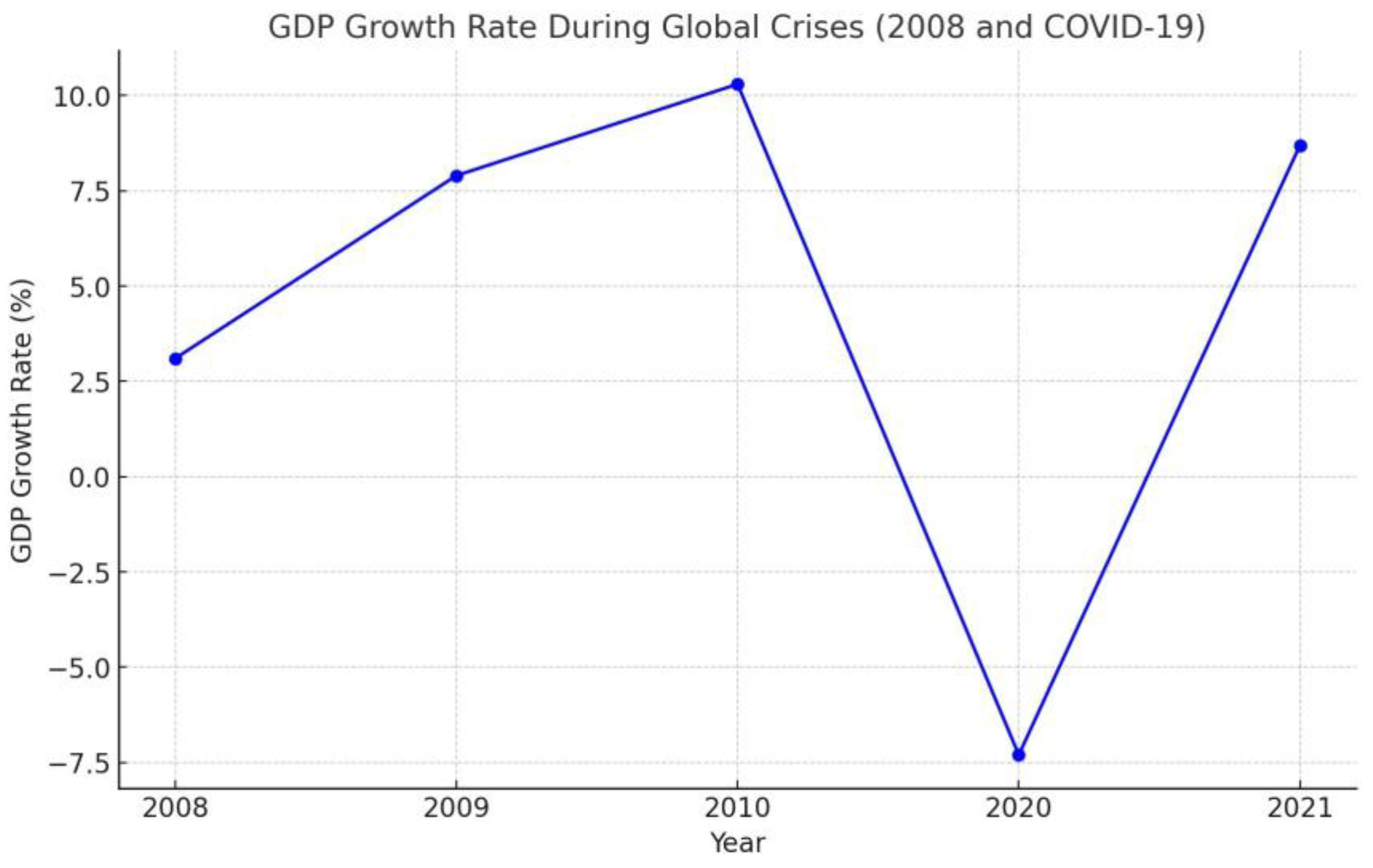
Figure 2.
Oil Price Fluctuations (2000–2024).
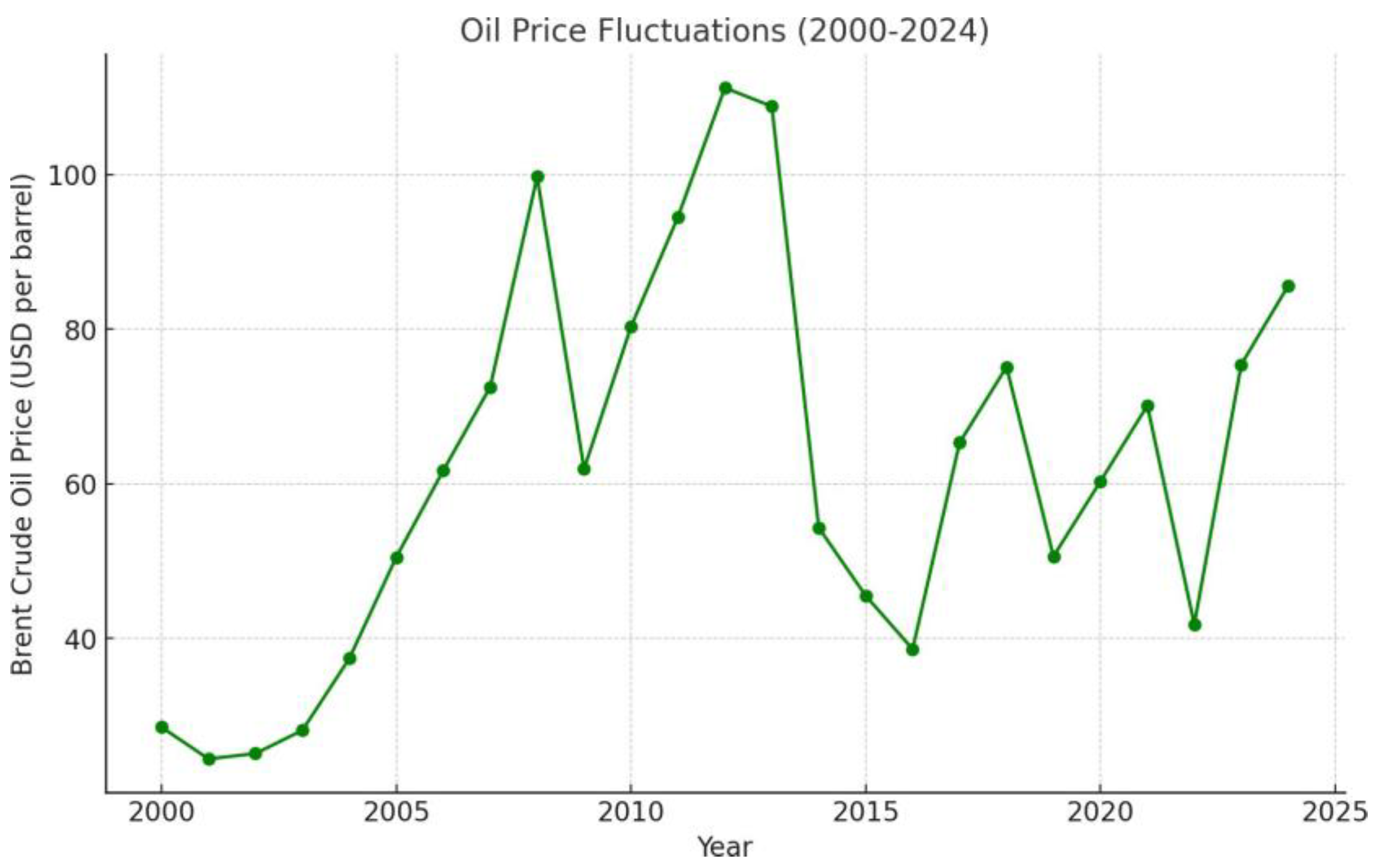
Figure 3.
Illustrates India's comparative economic downturns during crises. Source: IMF, World Economic Outlook, April 2021.
Figure 3.
Illustrates India's comparative economic downturns during crises. Source: IMF, World Economic Outlook, April 2021.
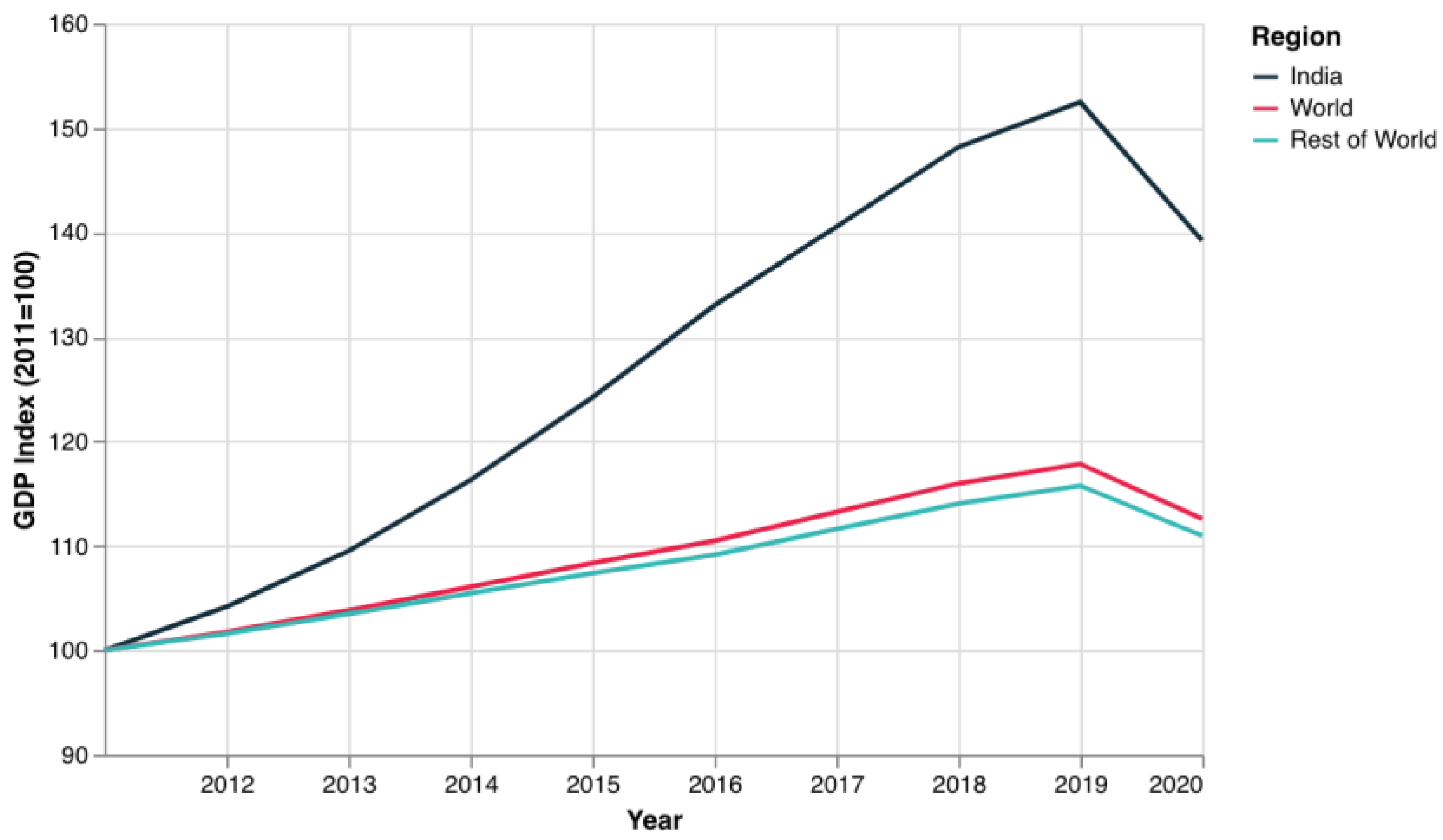
Figure 4.
Quantile regression estimates showing heterogeneous effects of oil and exchange-rate shocks across the conditional distributions.
Figure 4.
Quantile regression estimates showing heterogeneous effects of oil and exchange-rate shocks across the conditional distributions.
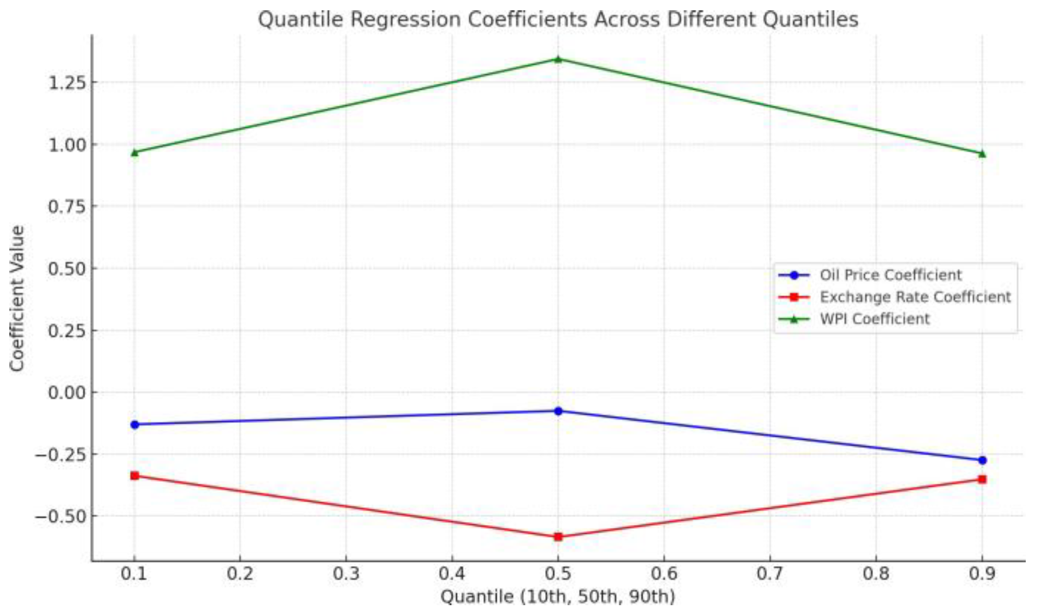
Figure 5.
Stability Test- IIP.

Figure 6.
stability test -Exchange Rate.
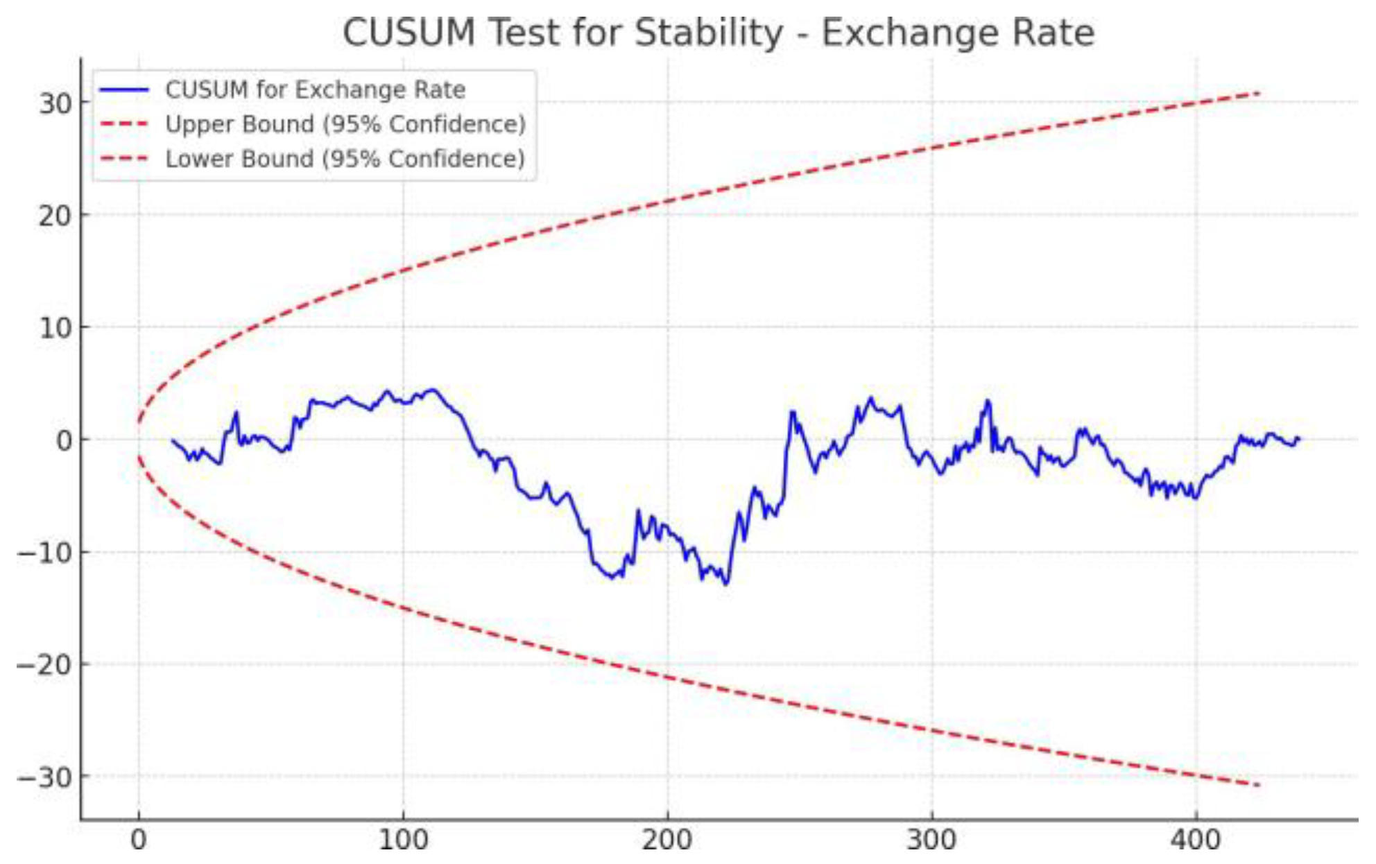
Figure 7.
Stability Test- WPI.
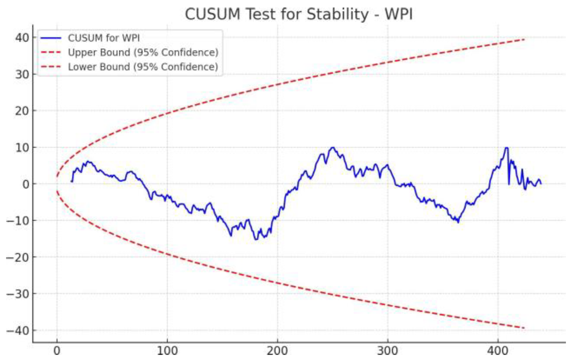
Figure 8.
Stability test for Oil Prices. Source: Author’s calculation.
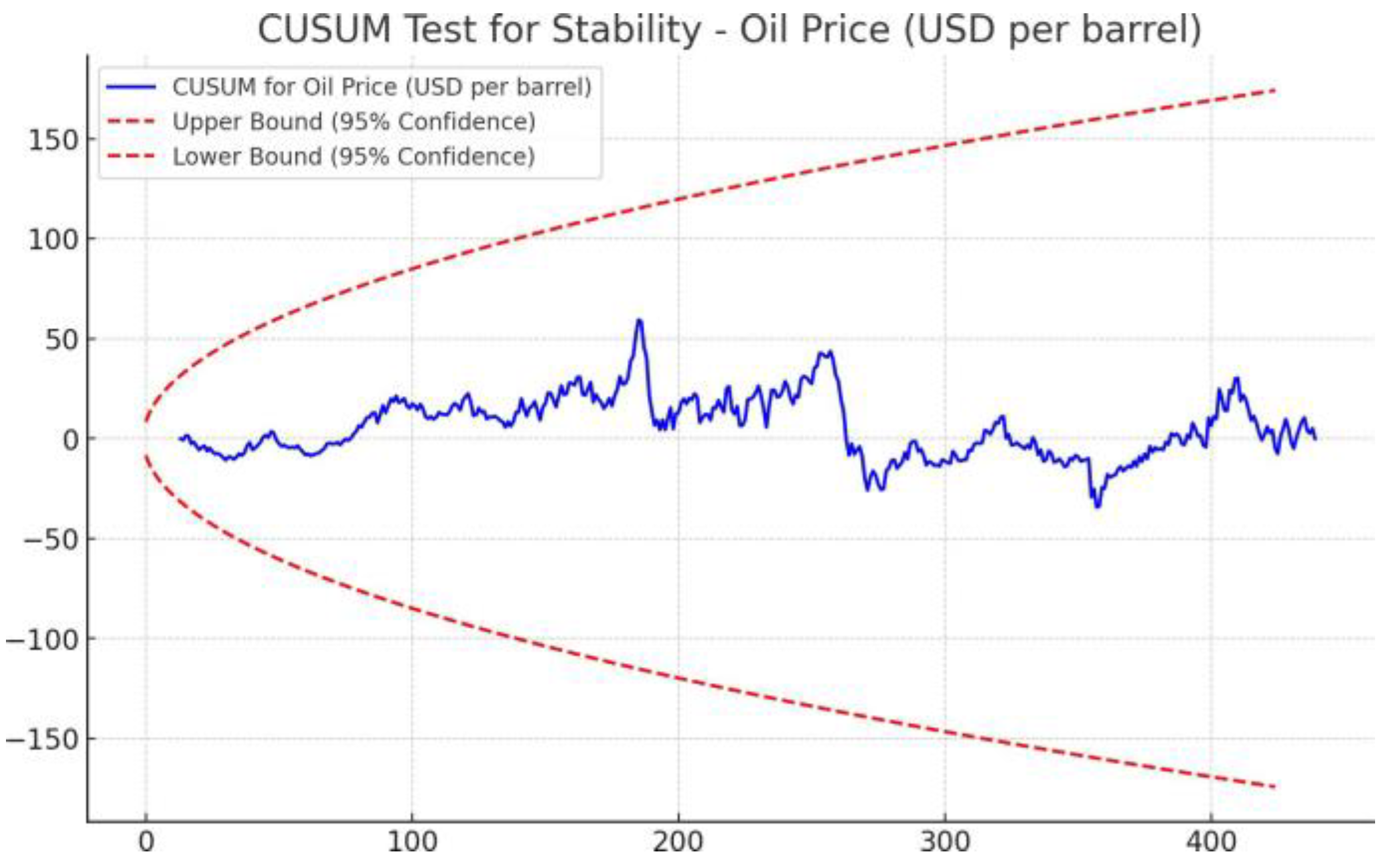
Table 1.
Key Macroeconomic Indicators During Global Crises.
| Macroeconomic Indicators | Description (%) |
|---|---|
| GDP Growth Rate (%) | 6.7% |
| IIP Growth Rate (%) | 2.6% |
| WPI Inflation (%) | 8.4% |
| Exchange Rate (INR/ USD) | 47.5% |
Source: Economic Survey (2008-2009), Ministry of Statistics and Programme Implementation (MOSPI), Office of the Economic Adviser, Ministry of Commerce and Industry, India.
Table 2.
Descriptive statistics.
| Variables | Mean | Standard Deviation s | Minimum | Maximum | Skewness | Kurtosis |
|---|---|---|---|---|---|---|
| IIP | 91.83 | 37.46 | 28.03 | 160.0 | -0.22 | -1.36 |
| Exchang e rate | 55.46 | 15.52 | 30.83 | 83.87 | 0.17 | -1.27 |
| WPI | 91.26 | 36.47 | 33.14 | 155.4 | 0.01 | -1.28 |
| Oil | 54.97 | 28.34 | 11.35 | 133.88 | 0.29 | -0.86 |
Source: author’s calculations.
Table 5.
Lag selection criteria.
| Lag | AIC | SIC | HQIC |
|---|---|---|---|
| 0 | -2.45 | -2.20 | -2.33 |
| 1 | -5.92 | -5.40 | -5.70 |
| 2* | -6.20* | -5.55* | -5.90* |
| 3 | -6.15 | -5.30 | -5.75 |
| 4 | -6.10 | -5.00 | -5.60 |
Source: Author’s Calculation.
Table 6.
Zivot–Andrews test and Bai-perron Result.
| Variable | Zivot–Andrews | Test Statistic | Critical Values | Break Type | Bai-perron Break Dates |
|---|---|---|---|---|---|
| IIP | 2009 )financial Crises) | -5.12 | -4.80 | Trend and level | 2009,2020 |
| Exchange rate | 2013 (Taper Tantrum) | -5.34 | -4.82 | Levle shift | 2008,2013,2020 |
| WPI | 2008 (financial crises) | -5.01 | -4.78 | Trend Shift | 2008,2014,2020 |
| Oil Prices | 2020 (covid) | -5.80 | -4.85 | Level and Trend | 2008,2014,2020 |
Source: author’s Calculation.
Table 7.
Johansen Co-integration Test.
| Hypothesised Number of co-Integrated Equations | Trace Stats | Max Eigen Stats | Critical Values (95%) |
|---|---|---|---|
| None* | 89.00 | 35.00 | 55.25 |
| At most 1* | 54.00 | 28.91 | 35.01 |
| At most 2 | 25.08 | 14.50 | 18.4 |
| At most 3 | 10.57 | 10.57 | 3.84 |
Source: author’s Calculation.
Table 8.
Gregory–Hansen Test for Co-integration with Structural Breaks.
| Variable | Test | Test Statistic | Critical Value | Break Date |
|---|---|---|---|---|
| IIP – WPI – ER – OP | ADF | -6.12 | -5.45 | Apr 2020 |
| IIP – WPI – ER – OP | Phillips Zt statistic, | -6.05 | -5.23 | Sept 2008 |
| IIP – WPI – ER – OP | Phillips Za statistic | -64.8 | -58.4 | March 2020 |
Source: author’s Calculation.
Table 10.
Impulse Response Functions (IRFs): Response of IIP to a shock in Oil Price (OP).
| Horizon | % Change in IIP |
|---|---|
| 1 | -0.18 |
| 3 | -0.35 |
| 6 | -0.28 |
| 12 | -0.10 |
Table 11.
Table IRF-B. Response of WPI to a shock in Oil Price (OP).
| Horizon | % Change in WPI |
|---|---|
| 1 | 0.10 |
| 3 | 0.25 |
| 6 | 0.19 |
| 12 | 0.07 |
Table 12.
Table IRF-C. Response of Exchange Rate (INR/USD) to a shock in Oil Price.
| Horizon | % Change In Exchange Rate |
|---|---|
| 1 | 0.40 |
| 3 | 0.80 |
| 6 | 0.55 |
| 12 | 0.20 |
Table 13.
IRF-D. Response of IIP to a shock in Exchange Rate (ER depreciation).
| Horizon | % Change in IIP |
|---|---|
| 1 | -0.06 |
| 3 | -0.14 |
| 6 | -0.11 |
| 12 | -0.04 |
Table 14.
FEVD-IIP. Variance shares for IIP.
| Horizon | IIP | Oil | Exchange Rate | WPI |
|---|---|---|---|---|
| 1 | 82 | 10 | 5 | 3 |
| 3 | 60 | 18 | 12 | 10 |
| 6 | 52 | 22 | 15 | 11 |
| 12 | 47 | 28 | 15 | 10 |
Table 15.
FEVD-WPI. Variance shares for WPI.
| Horizon | WPI | Oil | Exchange Rate | IIP |
|---|---|---|---|---|
| 1 | 70 | 18 | 7 | 5 |
| 3 | 52 | 30 | 10 | 8 |
| 6 | 46 | 34 | 11 | 9 |
| 12 | 43 | 35 | 12 | 10 |
Table 16.
FEVD-ER. Variance shares for Exchange Rate (INR/USD).
| Horizon | Exchange Rate | Oil | WPI | IIP |
|---|---|---|---|---|
| 1 | 78 | 12 | 6 | 4 |
| 3 | 64 | 18 | 10 | 8 |
| 6 | 60 | 20 | 11 | 9 |
| 12 | 58 | 20 | 12 | 10 |
Table 18.
ARCH LM Results.
| Variable | LM Statistic | P-Value | Conclusion |
|---|---|---|---|
| IIP | 23.38 | 0.00 | Presence of volatility |
| Exchange rate | 41.92 | 0.00 | Presence of volatility |
| WPI | 35.75 | 0.00 | Presence of volatility |
| Oil Price | 42.36 | 0.00 | Presence of volatility |
Source: Author Calculation.
Table 19.
GARCH(1,1) Estimates.
| Variable | Constant | ARCH Term | GARCH term | α+β |
|---|---|---|---|---|
| IIP | 0.00 | 0.21 | 0.72 | 0.93 |
| Exchange Rate | 0.00 | 0.18 | 0.76 | 0.94 |
| WPI | 0.00 | 0.25 | 0.58 | 0.93 |
| Oil Price | 0.00 | 0.30 | 0.62 | 0.92 |
Source: Author Calculation.
Table 20.
Robust Standard Errors: test for hetroscedasticity.
| Variable | Coefficient | Standard Error | T-Stats | P-Value |
|---|---|---|---|---|
| Constant | 31.73 | 6.69 | 4.74 | 0.00 |
| Exchange rate | —1.27 | 0.21 | -5.95 | 0.00 |
| WPI | 1.56 | 0.09 | 15.92 | 0.00 |
| Oil Price | -0.22 | 0.05 | -3.81 | 0.00 |
Source: author’s calculations.
Table 21.
Durbin-Watson Test.
| Variable | D-Stats | Lower Bound | Upper Bound | Results |
|---|---|---|---|---|
| IIP | 1.984 | 1.5 | 2.5 | No AC |
| Exchange rate | 1.988 | 1.5 | 2.5 | No AC |
| WPI | 2.060 | 1.5 | 2.5 | No AC |
| Oil Price | 1.973 | 1.5 | 2.5 | No AC |
Source: Author’s Calculations.
Disclaimer/Publisher’s Note: The statements, opinions and data contained in all publications are solely those of the individual author(s) and contributor(s) and not of MDPI and/or the editor(s). MDPI and/or the editor(s) disclaim responsibility for any injury to people or property resulting from any ideas, methods, instructions or products referred to in the content. |
© 2026 by the authors. Licensee MDPI, Basel, Switzerland. This article is an open access article distributed under the terms and conditions of the Creative Commons Attribution (CC BY) license (http://creativecommons.org/licenses/by/4.0/).
Copyright: This open access article is published under a Creative Commons CC BY 4.0 license, which permit the free download, distribution, and reuse, provided that the author and preprint are cited in any reuse.


