Submitted:
26 December 2025
Posted:
31 December 2025
You are already at the latest version
Abstract
Models of neutron and strange stars are considered in the approximation of a uniform density distribution. A universal algebraic equation, valid for any equation of state, is used to find the approximate mass of a star of a given density without resorting to the integration of differential equations. Equations of state for neutron stars had been taken for degenerate neutron gas and for more realistic ones, used by Bethe, Malone, Johnson (1975). Models of homogeneous strange stars for the equation of state in the "quark bag model" have a simple analytical solution. The solutions presented in the paper for various equations of state differ from the exact solutions obtained by the numerical integration of differential equations by at most ∼ 20%. The formation of strange stars is examined as a function of the deconfinement boundary (DB), at which quarks become deconfined. Existing experimental data indicate that matter reaches very high densities in the vicinity of the DB. This imposes strong constraints on the maximum mass of strange stars and prohibits their formation at the final stages of stellar evolution, because the limiting mass of neutron stars is substantially higher and corresponds to considerably lower matter densities.
Keywords:
strange stars
; uniform model
; general relativity
1. Introduction
The first conclusion about the existence of an upper mass limit for cold stars, the equilibrium of which is maintained by the pressure of degenerate electrons, was made by Stoner [1], who considered the model of a white dwarf of uniform density. He generalized the consideration of the pressure of degenerate electrons, made in [2,3], to the case of high density under conditions of ultra-relativistic degeneracy, and obtained the limit for . To refine the maximum mass of observed white dwarfs, Chandrasekhar [4], following Stoner [1], used = 2.5, but considered the structure of the star from Emden polytropic model at , and obtained . From the theory of stellar evolution, as well as from observations, it follows that almost all white dwarfs consist of a mixture of carbon 12 and oxygen 16 for which [5] and . This realistic value was first obtained by Landau [6], who worked independently of Stoner and Chandrasekhar.
In this paper, we construct approximate models of cold neutron and strange stars of arbitrary mass assuming a uniform density distribution by using algebraic equations derived from the general theory of relativity (GTR) . Within this model, all results, including the values of the limiting masses of neutron stars (NSs), are obtained analytically, from algebraic equations we derived in [7] (see also [8]), for any equations of state. A simple analytical solution is obtained for the equation of state in the popular quark bag model [9].
2. Uniform-Density Neutron Stars
To construct realistic models of NS and SS, it is necessary to use general relativity, since the gravitational potential reaches tenths of and the NS radius is only a few gravitational radii . The models of non-rotating NSs are constructed using a Schwarzschild-type metric [10,11]
where
In general relativity, a total density of matter is considered, which includes the total rest energy density and internal energy . The mass M is the total gravitating mass, which includes the gravitational energy; therefore, the total energy of an NS is and the total energy e inside a radius r is . From the general relativity equations it follows that the baryon density n is related to the number of baryons (quarks) inside the radius r, as [12]
where - is the baryonic rest mass in the NS.
For a uniform star and do not depend on the radius, the integral in expression (3) is calculated analytically [13]
To relate the NS radius R to the density , it is necessary to find the extremum of the function at a fixed value of the number of baryons in the star N, which are written as
Differentials and are a liner combination of differentials and . For a fixed number of baryons, with , we obtain a linear connection between and , and connection . The equilibrium condition
gives us the following algebraic equation for the equilibrium of the uniform barotropic NS or SS star in GR [7]
where
Figure 1 shows the dependence , determined by equation (7).When the denominator on the right-hand side of (7) decreases to zero, the ratio and the density tend to infinity. The abscissa of the vertical dashed line in Figure 1 corresponds to the zero root of the denominator of (7), . The horizontal dash-dotted line separates the physically permissible region from the upper region, where the principle of causality is violated, according to which the speed of sound in matter cannot exceed the speed of light.
3. Construction of the Equilibrium Curve for a Uniform Density Model
The dependences or and can be built using the following procedure.
1. Select an equation of state or given by formulas or tables.
2. Set the ratio of the gravitational radius of the star to the physical radius: .
3. Find the ratio of pressure to density for this value of x.
4. Find the value of the density from the equation of state.
5. Find the radius of the model from the definition of x in the form .
6. Finally, find the mass of the uniform-density model, .
The calculation results for several equations of state are presented in Figure 2, Figure 3 and Figure 4 from [7], which also include the dependence of for arbitrary density distribution, obtained by solving the Oppenheimer-Volkoff equations [14].
A comparison of results for uniform density models with exact solutions of differential equations of equilibrium for various equations of state, including some from Bethe et al.(1975) [15] shows that the approximate value of the critical mass of a star exceeds the exact value by at most . Critical densities in the uniform density models turn out to be significantly lower than the values of central densities in numerical models and are comparable with average densities of these models.
4. Uniform-Density Strange Stars
In [9], it was suggested that strange matter containing the strange s-quark could have zero pressure at a density close to that of nuclear matter. This hypothesis was formalized using the MIT bag model, within which the corresponding equation of state is written in the form [9]:
where parameter B defines density at which pressure equals to zero .
Solution of algebraic equilibrium equation at this EOS can be obtained by substituting EOS (10) in (7) and can be written in the form [16]
Here
where functions are determined by Equation (8). Using (10), we obtain dependencies for homogeneous strange stars, presented in Figure 5, Figure 6 from [16]
Equilibrium state follows from the equation
which is reduced to finding of the extremum of the function
and is defined by the equation
The result of the numerical solution of this equation is , which is valid for all values of the parameter B in EOS. This value determines the critical parameters as function of B. In all models the loss of stability happens at the ratio , for all values of the parameter B. The dependence of the function is shown at Figure 7.
Critical parameters as function of B can be written in the form:
Critical parameters of SS in the case of uniform density distribution are given in Table 1.
For the point of maximum mass, similar dependences were obtained in [9] by numerically solving the Oppenheimer-Volkov equation [14], see also [17]. To compare uniform and nonuniform density models of SS, models of cold SS were constructed for the case of a nonuniform density distribution, by integration of the Oppenheimer-Volkoff equation with the MIT bag equation of state. Figure 8, Figure 9 and Figure 10 show the mass-radius dependences for models with uniform density distribution and for the exact ones for different bag constants. The values at which nonuniform stars lose stability are given in Table 2.
5. Strange Stars and Confinement
The Standart model contains six flavors of quarks , named up , down , strange , charm , bottom , and top . Quark flavor properties are shown in Table 3. Baryons containing one or more strange quarks but not having charm , bottom or top quarks, are called hyperons. Hyperons may exist in a stable form within neutron stars’ cores. Some types of hyperons and their properties are shown in Table 4.
5.1. Experimental Estimations
Energy density in the SPS CERN head-on experiments for transition to quark-gluon plasma (QGP), was estimated as about 3 GeV/fm3 [18]. Experimental data from heavy ion collider, RHIC, gave estimation for lower limit for QGP formation as [19]. It was obtained from data on PHENIX (RHIC) that the energy density at the point of QGP formation is at least [20]. In the experiment on LHC [21], the central energy density during formation of QGP in Pb+Pb collisions was estimated as .
5.2. Theoretical Estimations
Numerous theoretical investigation with simplifying assumption had been performed during 30 years. Their results for QGP formation border are scattered between , what is more then an order of magnitude lower than the experimantal results. It seems that the theory needs farther improvements, probably in choosing a more complicated models.
6. Conclusions
From comparison of the parameters in the calculated models with experimental results we see that the results for values of B could be considered as realistic only for maximal values of B, and even larger. At large B the loss of stability of a strange star happens at mass , what is much lower than the maximum neutron star masses for all equation of states. We could conclude therefore, that strange stars are not forming in the process of stellar evolution. A matter density in strange stars is comparable with the density at very early stages of universe expansion, where we could expect formation of SS at different masses without connection with stellar evolution. We may call it as Primordial Strange Stars (PSS) in analogy with Primordial Black Hole (PBH), in the case if both of them are real.
References
- E.C. Stoner , London, Edinburgh Dublin Philos. Mag.J. Sci.: Ser. 7 9 (60), 944 (1930).
- R. H. Fowler, Mon. Not. R. Astron. Soc. 87, 114 (1926).
- J. Frenkel , Zeitschr. Phys. 50, 234 (1928).
- S. Chandrasekhar, Astrophysical Journal. 74, 81 (1931).
- E.L. Schatzman, White dwarfs. Amsterdam. North Holland (1958).
- L.D. Landau , Phys. Zs. Sowjet. 1, 285 (1932).
- Bisnovatyi-Kogan G.S., Patraman E.A. Astronomy Reports 67, 824 (2023).
- Naurenberg M., Chapline G., Jr. ApJ, 179, 277 (1973).
- E. Witten, Phys. Rev. D30, 272 (1984).
- L. D. Landau and E. M. Lifshitz, Course of Theoretical Physics, Vol. 2: The Classical Theory of Fields (Pergamon, Oxford, 1975; Fizmatgiz, Moscow, 2001).
- Ya. B. Zel’dovich and I. D. Novikov, The Theory of the Gravitation and Stars Evolution (Nauka, Moscow, 1971) [in Russian].
- G. S. Bisnovatyi-Kogan, Physical Problems in the Theory of Stellar Evolution (Nauka, Moscow, 1989) [in Russian].
- I. S. Gradshteyn, I. M. Ryzhik, Table of integrals, series and products. New York: Academic Press, edited by Geronimus, Yu.V., Tseytlin, M.Yu. (4th ed.). (1965).
- Oppenheimer J. R, and Volkoff G. M. Physical Review.- 1939. - Vol.55. - P.374-381.
- R. C. Malone, M. B. Johnson, and H. A. Bethe, Astrophys. J. 199, 741 (1975).
- Bisnovatyi-Kogan G.S., Patraman E.A. Astronomy Reports (in press).
- Naurenberg M., Chapline G., Jr. Nature, 264, 235 (1976).
- T. Alber, et al., Phys. Rev. Lett. 75 (1995) 3814.
- Arsene I, et al. Nucl. Phys. A 757:1 (2005).
- Adcox K, et al. Nucl. Phys. A 757:184 (2005).
- J. Adam, D. Adamová, M. M. Aggarwal, G. Aglieri Rinella, M. Agnello, N. Agrawal, Z. Ahammed, S. Ahmad, S. U. Ahn, Phys. Rev. C 94, (2016).
Figure 1.
(Solid line) Dependence of on the parameter x , according to (7). The abscissa of the vertical dashed line corresponds to the zero root of the denominator of (7), . The horizontal dash-dotted line separates the physically admissible region from the upper region where the principle of causality is violated.
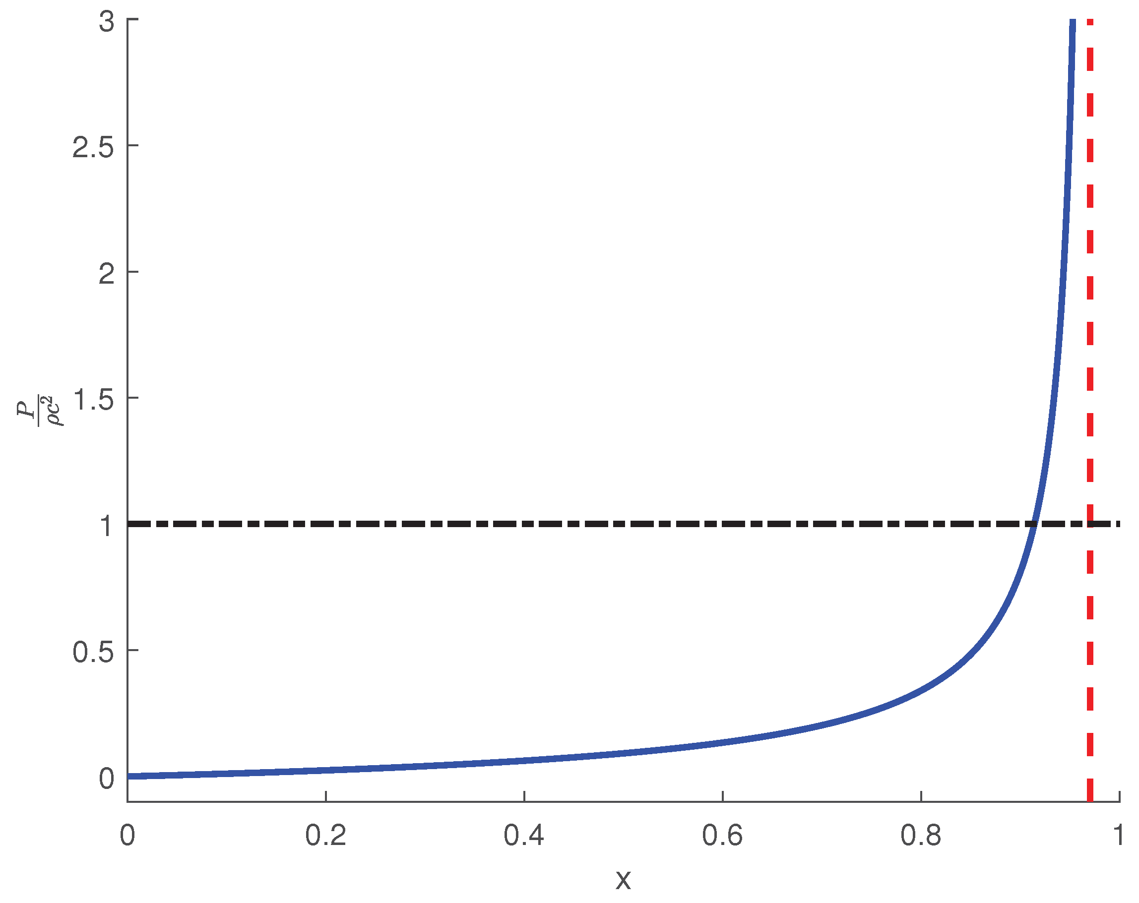
Figure 2.
Degenerate neutron gas: dependence in the case of a uniform density distribution (solid line), and the exact models (dash-dotted line); dependence (dashed line) in the case of uniform density and (dotted line) the exact model.
Figure 2.
Degenerate neutron gas: dependence in the case of a uniform density distribution (solid line), and the exact models (dash-dotted line); dependence (dashed line) in the case of uniform density and (dotted line) the exact model.
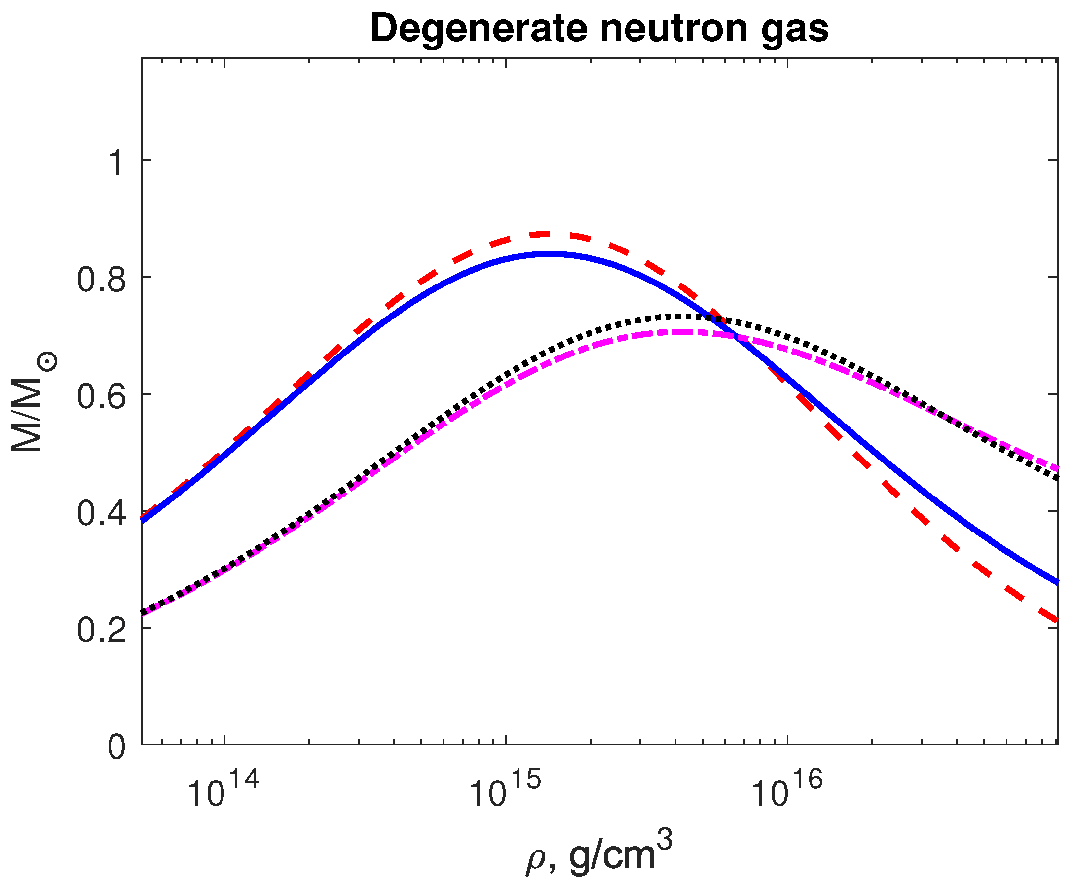
Figure 3.
Degenerate neutron gas with a correction for nuclear interaction: the dependence (solid line) in the case of a uniform density distribution and (dash-dotted line) the exact model; the dependence (dashed line) in the case of uniform density and (dotted line) in the exact model.
Figure 3.
Degenerate neutron gas with a correction for nuclear interaction: the dependence (solid line) in the case of a uniform density distribution and (dash-dotted line) the exact model; the dependence (dashed line) in the case of uniform density and (dotted line) in the exact model.
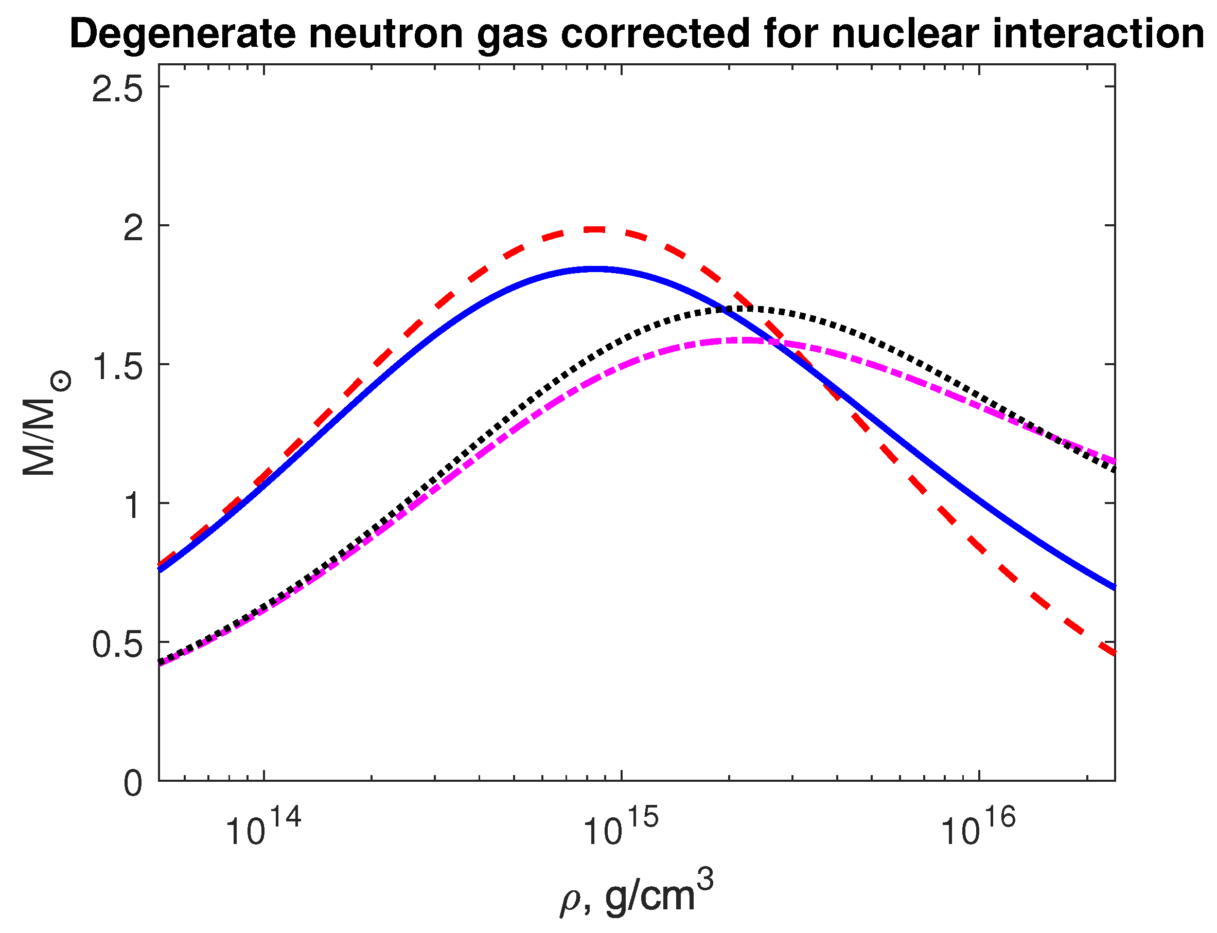
Figure 4.
Model I H. The dependence (solid line) in the case of a uniform density distribution and (dash-dotted line) in the exact model; the dependence (dashed line) in the case of a uniform density and (dotted line) in the exact model. The vertical solid line shows at what density and g/cm3.
Figure 4.
Model I H. The dependence (solid line) in the case of a uniform density distribution and (dash-dotted line) in the exact model; the dependence (dashed line) in the case of a uniform density and (dotted line) in the exact model. The vertical solid line shows at what density and g/cm3.
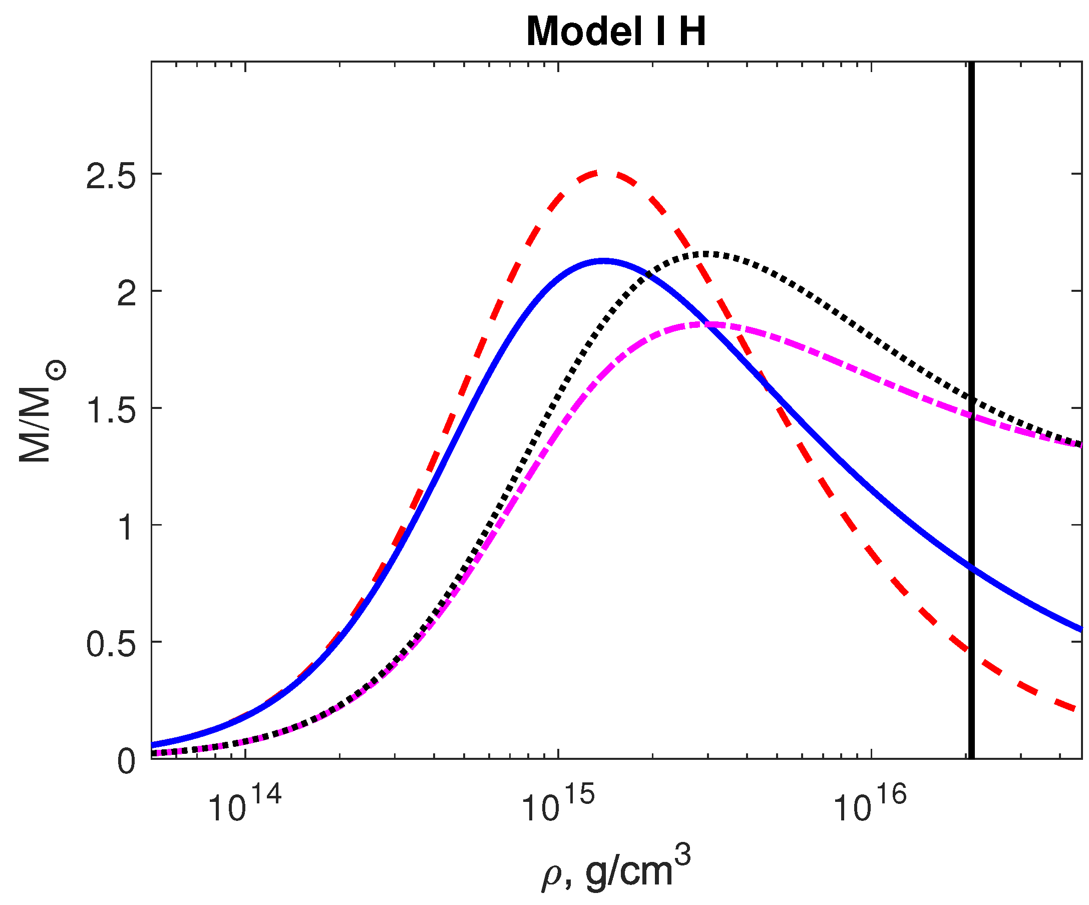
Figure 5.
Dependence of mass on density for different values of the bag constant B in the MIT bag model. Here B is given in units MeV/fm3. The curve maxima are indicated by crosses. The parameters of stars at maxima corresponding to critical states are presented in Table 1.
Figure 5.
Dependence of mass on density for different values of the bag constant B in the MIT bag model. Here B is given in units MeV/fm3. The curve maxima are indicated by crosses. The parameters of stars at maxima corresponding to critical states are presented in Table 1.
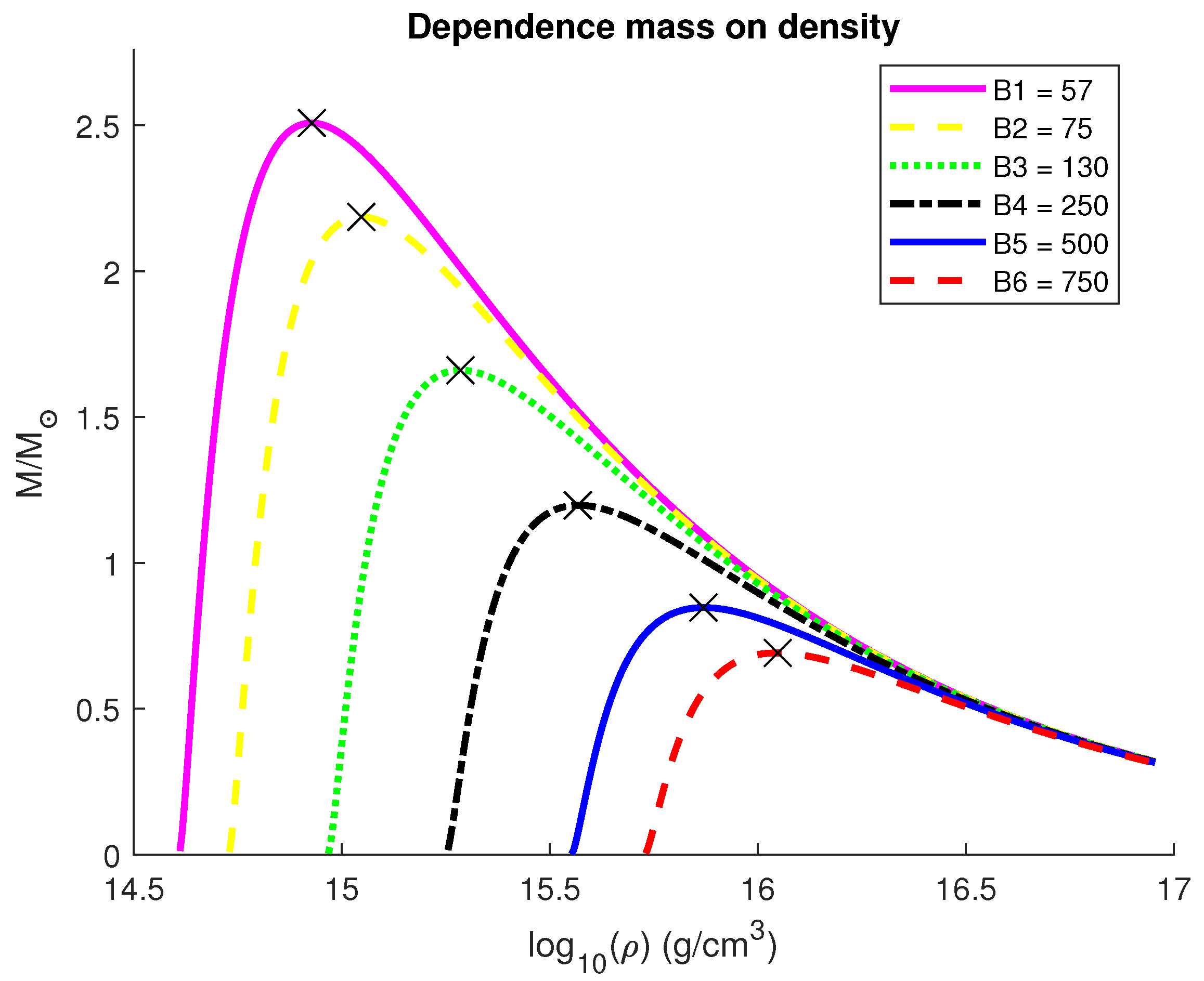
Figure 6.
Dependence of mass on radius for different values of the bag constant B in the MIT bag model. Here B is given in units MeV/fm3.
Figure 6.
Dependence of mass on radius for different values of the bag constant B in the MIT bag model. Here B is given in units MeV/fm3.
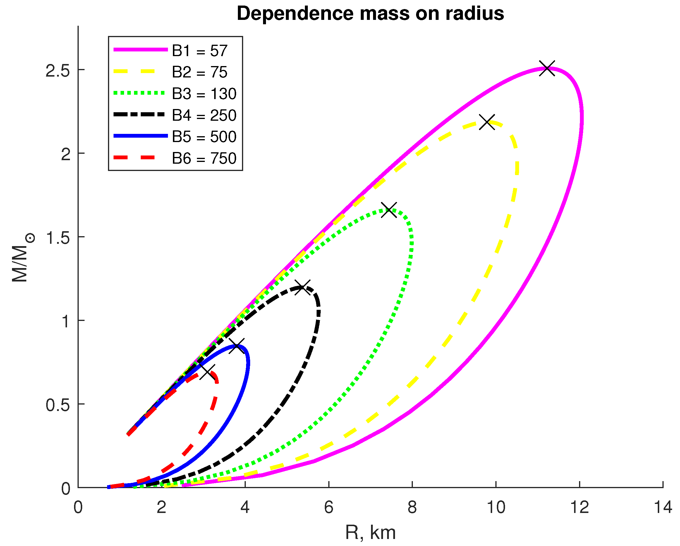
Figure 7.
Dependence . The maximum of the function is indicated by a cross, and its value is
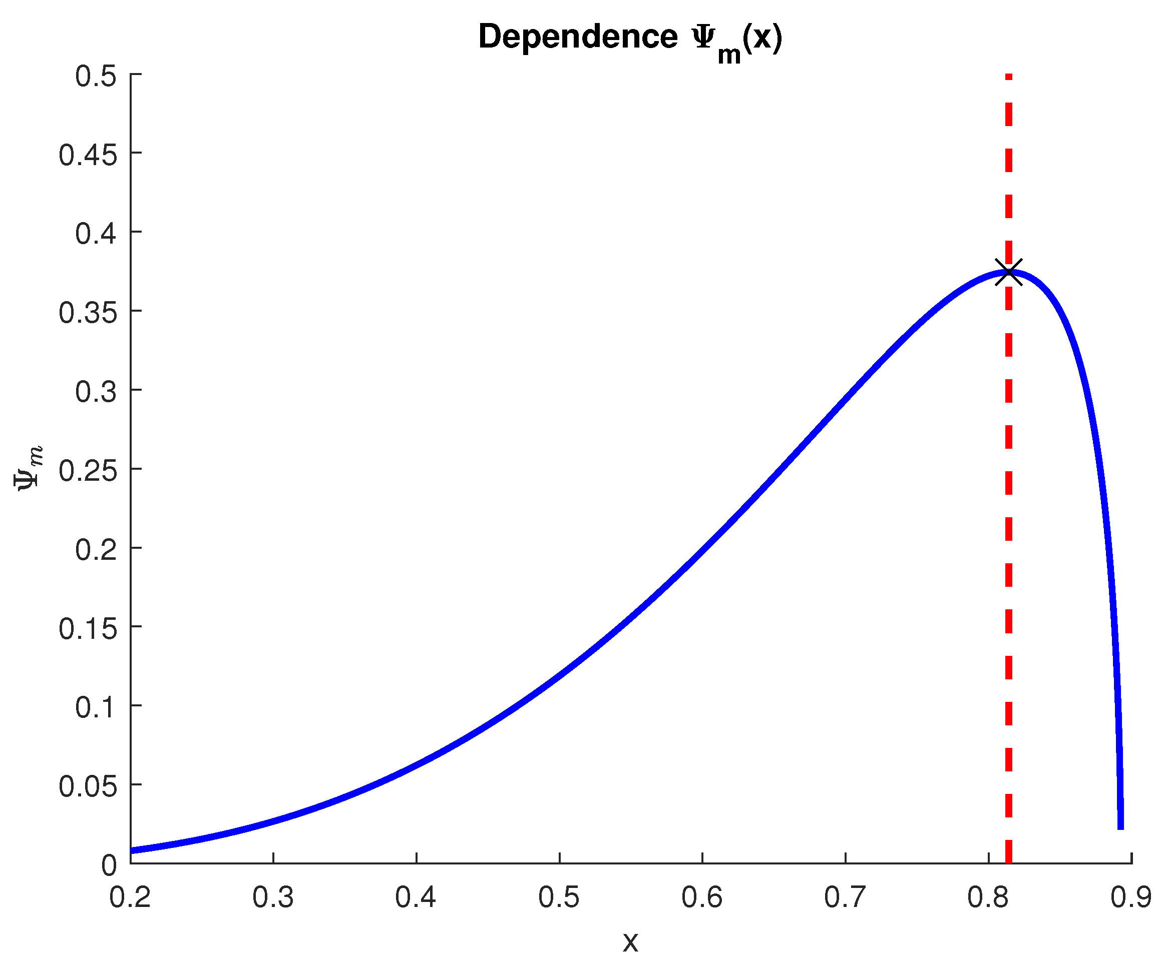
Figure 8.
Dependence for MeV/fm3. The solid red line shows the dependence for the uniform model, the dashed blue line shows the exact model. The curve maxima are indicated by crosses.
Figure 8.
Dependence for MeV/fm3. The solid red line shows the dependence for the uniform model, the dashed blue line shows the exact model. The curve maxima are indicated by crosses.
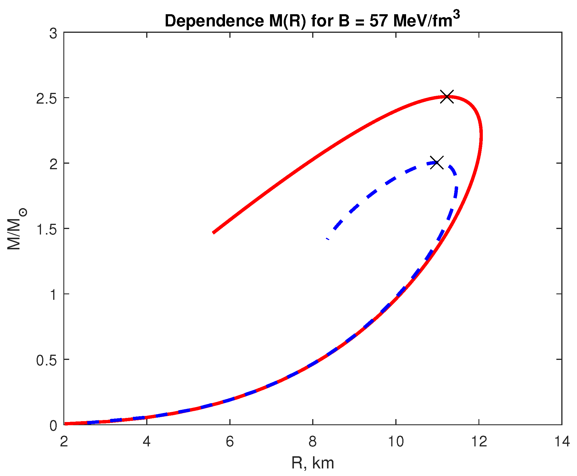
Figure 9.
Dependence for MeV/fm3. The solid red line shows the dependence for the uniform model, the dashed blue line shows the exact model. The curve maxima are indicated by crosses.
Figure 9.
Dependence for MeV/fm3. The solid red line shows the dependence for the uniform model, the dashed blue line shows the exact model. The curve maxima are indicated by crosses.
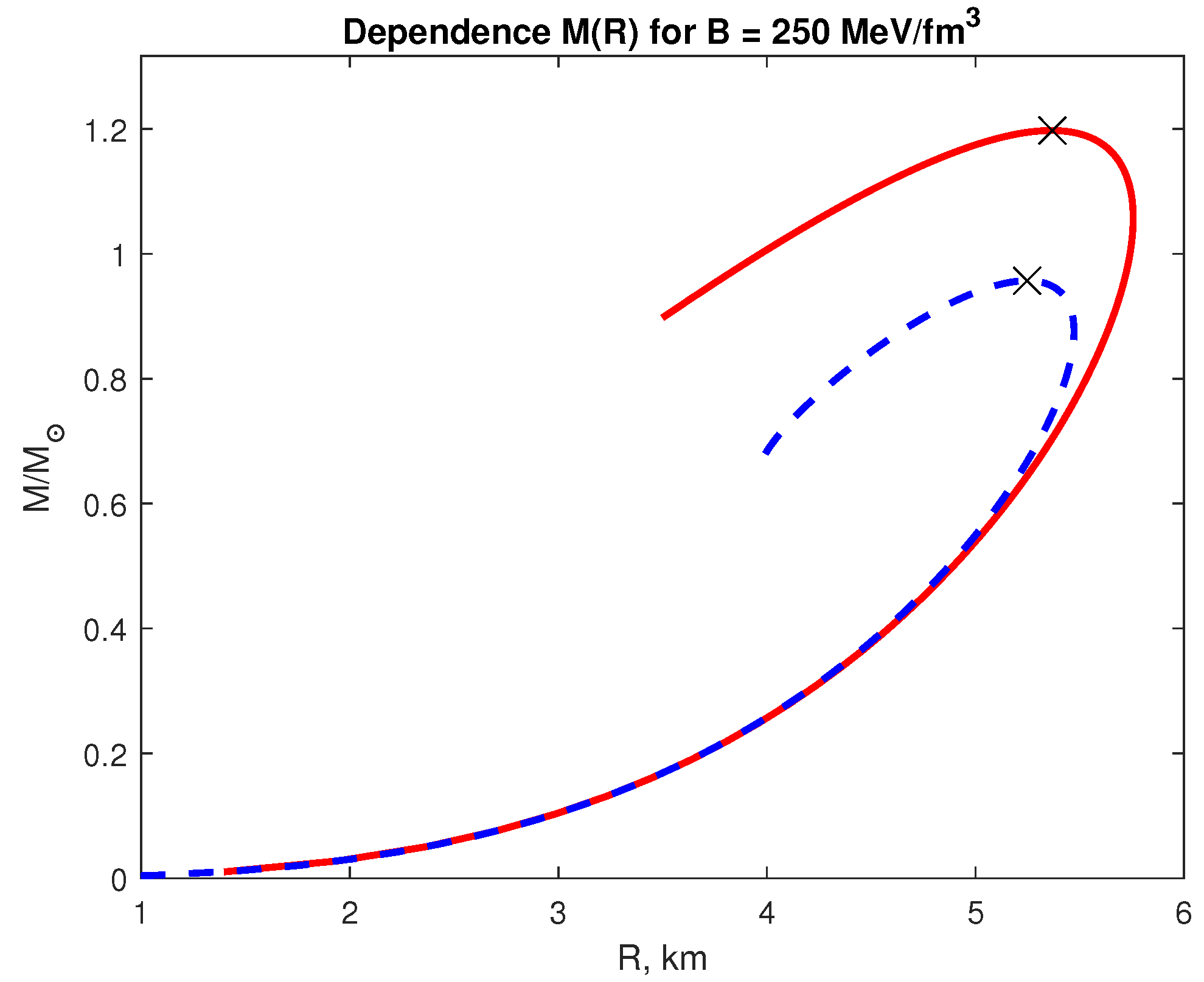
Figure 10.
Dependence for MeV/fm3. The solid red line shows the dependence for the uniform model, the dashed blue line shows the exact model. The curve maxima are indicated by crosses.
Figure 10.
Dependence for MeV/fm3. The solid red line shows the dependence for the uniform model, the dashed blue line shows the exact model. The curve maxima are indicated by crosses.
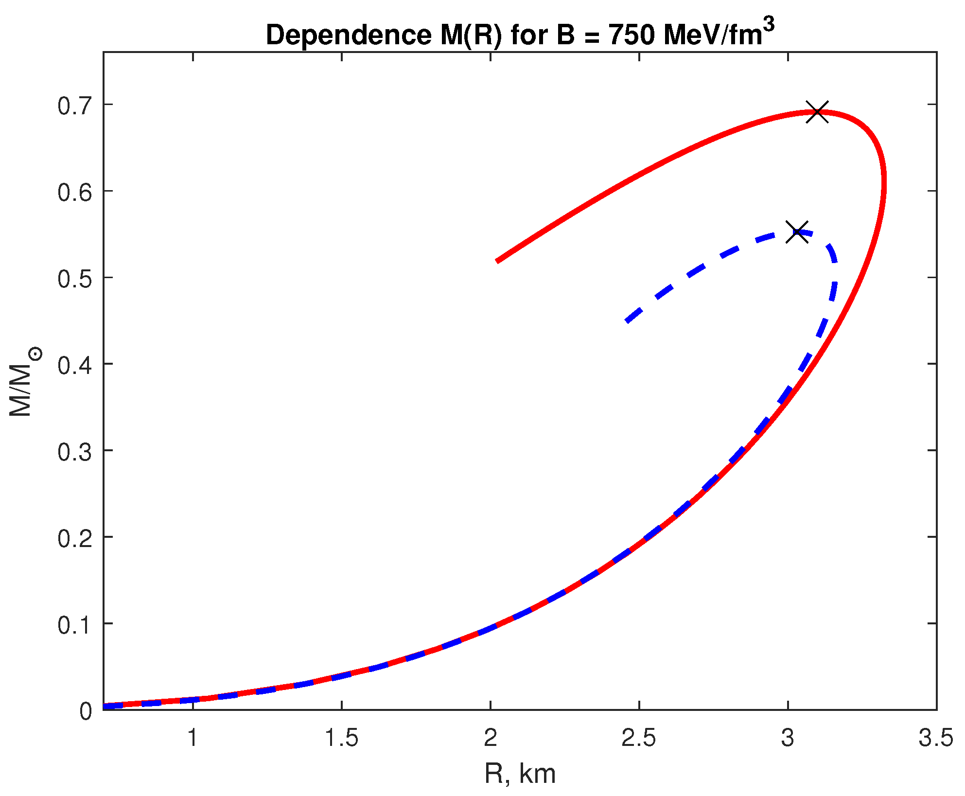

Table 1.
Critical parameters of homogeneous strange stars for different B. The density of the deconfinement point is defined by equation g/cm3. To convert units of measurement to CGS, it is required to use .
Table 1.
Critical parameters of homogeneous strange stars for different B. The density of the deconfinement point is defined by equation g/cm3. To convert units of measurement to CGS, it is required to use .
| B, MeV/fm3 | , g/cm3 | , g/cm3 | R, km | |
|---|---|---|---|---|
| 57 | 0.4 | 2.51 | 0.839 | 11.25 |
| 75 | 0.53 | 2.19 | 1.106 | 9.81 |
| 130 | 0.93 | 1.66 | 1.919 | 7.45 |
| 250 | 1.78 | 1.2 | 3.703 | 5.36 |
| 500 | 3.56 | 0.85 | 7.372 | 3.8 |
| 750 | 5.35 | 0.69 | 11.15 | 3.09 |
Table 2.
Critical parameters of exact model for different B. g/cm3 is a density of the deconfinement point. To convert units of measurement to CGS, it is required to use .
Table 2.
Critical parameters of exact model for different B. g/cm3 is a density of the deconfinement point. To convert units of measurement to CGS, it is required to use .
| B, MeV/fm3 | , g/cm3 | , g/cmm3 | R, km | |
|---|---|---|---|---|
| 57 | 0.4 | 2 | 1.96 | 11 |
| 75 | 0.53 | 1.75 | 2.58 | 9.58 |
| 130 | 0.93 | 1.33 | 4.44 | 7.28 |
| 250 | 1.78 | 0.96 | 8.62 | 5.25 |
| 500 | 3.56 | 0.68 | 17.17 | 3.71 |
| 750 | 5.35 | 0.55 | 25.8 | 3.03 |
Table 3.
Quark flavor properties (from Wikipedia)
| Particle | Mass* | J | B | Q | C | S | T | Antiparticle | ||||
|---|---|---|---|---|---|---|---|---|---|---|---|---|
| Name | Symbol | [MeV/] | [ℏ] | [e] | Name | Symbol | ||||||
| First generation | ||||||||||||
| up | u | 0 | 0 | 0 | 0 | antiup | ||||||
| down | d | 0 | 0 | 0 | 0 | antidown | ||||||
| Second generation | ||||||||||||
| charm | c | 0 | 0 | 0 | 0 | anticharm | ||||||
| strange | s | 0 | 0 | 0 | 0 | antistrange | ||||||
| Third generation | ||||||||||||
| top | t | 0 | 0 | 0 | 0 | antitop | ||||||
| bottom | b | 0 | 0 | 0 | 0 | antibottom | ||||||
J - total angular moment, B - baryon number, Q - electric charge, - isospin, C - charm, S - strangeness, T - topness, - bottomness.
Table 4.
Hyperons (from Wikipedia)
| Particle | Symbol | Makeup | Rest mass [MeV/] | Isospin, I | Spin parity, | |
|---|---|---|---|---|---|---|
| Lambda | uds | 1115.683(6) | 0 | 0 | ||
| Lambda resonance | uds | 0 | 0 | |||
| Lambda resonance | uds | 1519(1) | 0 | 0 | ||
| Sigma | uus | 1189.37(7) | 1 | +1 | ||
| Sigma | uds | 1192.642(24) | 1 | 0 | ||
| Sigma | dds | 1197.449(30) | 1 | |||
| Sigma resonance | uus | 1382.8(4) | 1 | +1 | ||
| Sigma resonance | uds | 1383.7(1.0) | 1 | 0 | ||
| Sigma resonance | dds | 1387.2(5) | 1 | |||
| Omega | sss | 1672.45(29) | 0 |
Disclaimer/Publisher’s Note: The statements, opinions and data contained in all publications are solely those of the individual author(s) and contributor(s) and not of MDPI and/or the editor(s). MDPI and/or the editor(s) disclaim responsibility for any injury to people or property resulting from any ideas, methods, instructions or products referred to in the content. |
© 2025 by the authors. Licensee MDPI, Basel, Switzerland. This article is an open access article distributed under the terms and conditions of the Creative Commons Attribution (CC BY) license.
Copyright: This open access article is published under a Creative Commons CC BY 4.0 license, which permit the free download, distribution, and reuse, provided that the author and preprint are cited in any reuse.


