Thermocapillary Effects in the Evaporation of Heated Sessile Droplets

1. Introduction

Inkjet printing is widely used to fabricate micro-electromechanical systems (MEMS), flexible electronics, and various miniaturized sensors, where picoliter- to microliter-scale droplets of functional inks are deposited as sessile droplets on a solid substrate [1,21]. Controlling the drying behavior of these droplets is critical because undesired internal flows can lead to highly non-uniform particle deposition, as illustrated qualitatively in Figure 1.

A well-known example is the coffee-ring effect: during evaporation of a sessile droplet with a pinned contact line, an outward capillary flow transports suspended particles toward the periphery, leaving a dense ring-like deposit and a depleted interior [1,5,21]. This non-uniform deposition reduces the electrical conductivity and reliability of printed conductive tracks and often requires additional post-processing steps to mitigate such as multiple printing passes or thermal annealing [19,21].

Substrate heating and the use of binary solvent mixtures provide a powerful strategy to counteract the coffee-ring effect [4,10,20]. In such systems, a more volatile component (e.g., water) evaporates faster, enriching the interface with a less volatile component (e.g., ethylene glycol or glycerol). The resulting surface tension gradients drive Marangoni flows that can oppose the outward capillary flow and redistribute particles toward the droplet center [7,20,21].

In recent years, several modeling approaches have been proposed to describe the evaporation of sessile single-component and multicomponent droplets [2,3,6]. These range from relatively simple diffusion-limited models with fixed geometry to fully coupled, time-dependent simulations that include hydrodynamics, heat transfer, and composition-dependent properties. Several recent studies have reported complementary insights into thermal transport and evaporation phenomena in micro- and nanoscale systems using both numerical and molecular approaches [13,14,15,16,17]. There is a clear need to relate these modeling levels to each other and to show when a simple model is sufficient and when an advanced model is required.

The present work contributes to this need by developing and validating an axisymmetric multiphysics model of reactive silver-ink droplet evaporation on a heated substrate. The study explicitly compares the predictions of simplified and advanced models, and it explains how key physical mechanisms—such as Marangoni circulation and contact-line pinning—modify the drying process and final deposit pattern [9,12,18].

2. Physical System and Modeling Framework

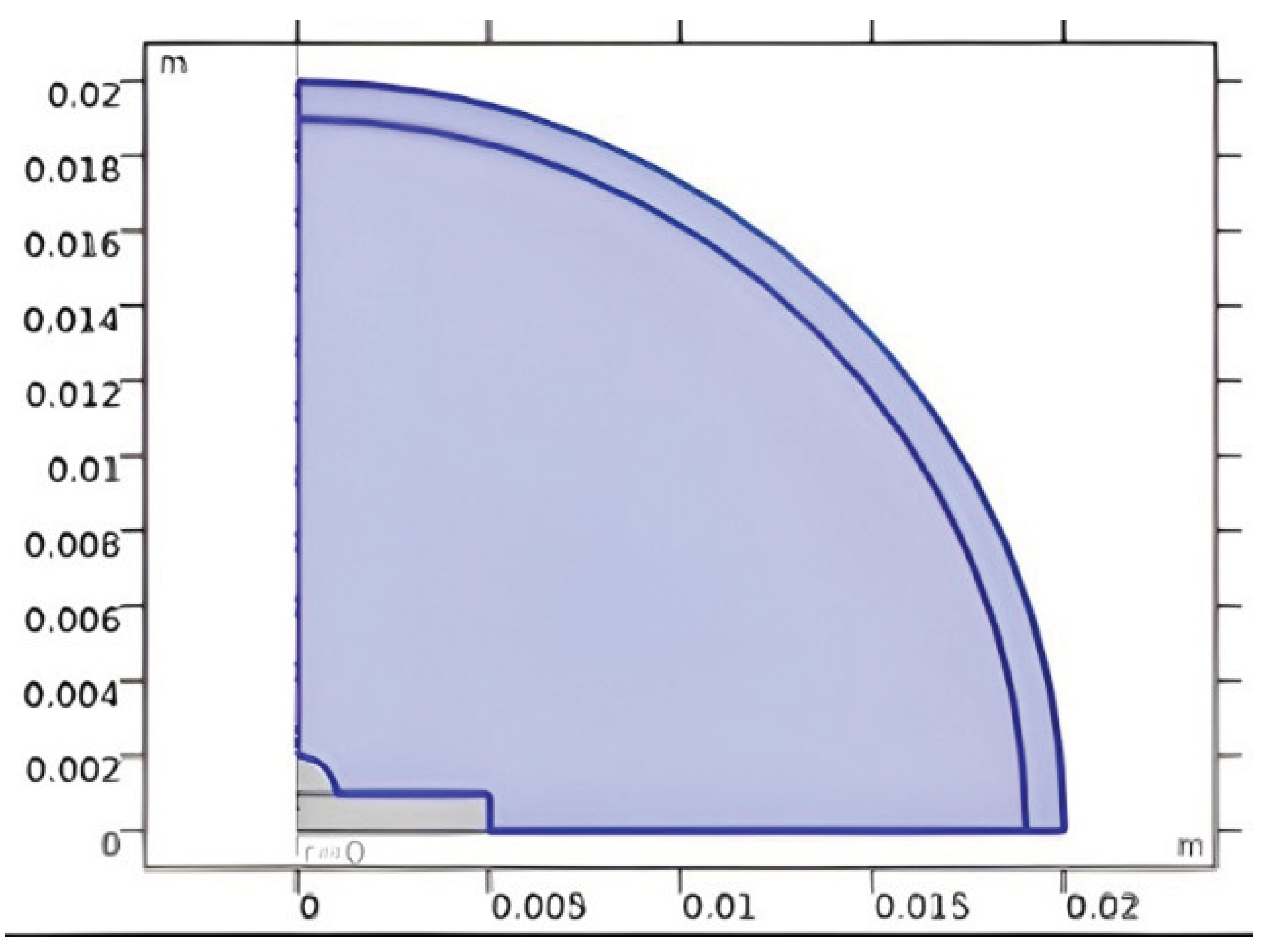
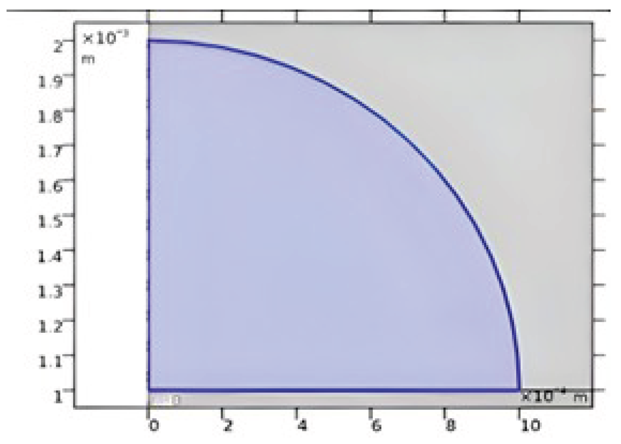
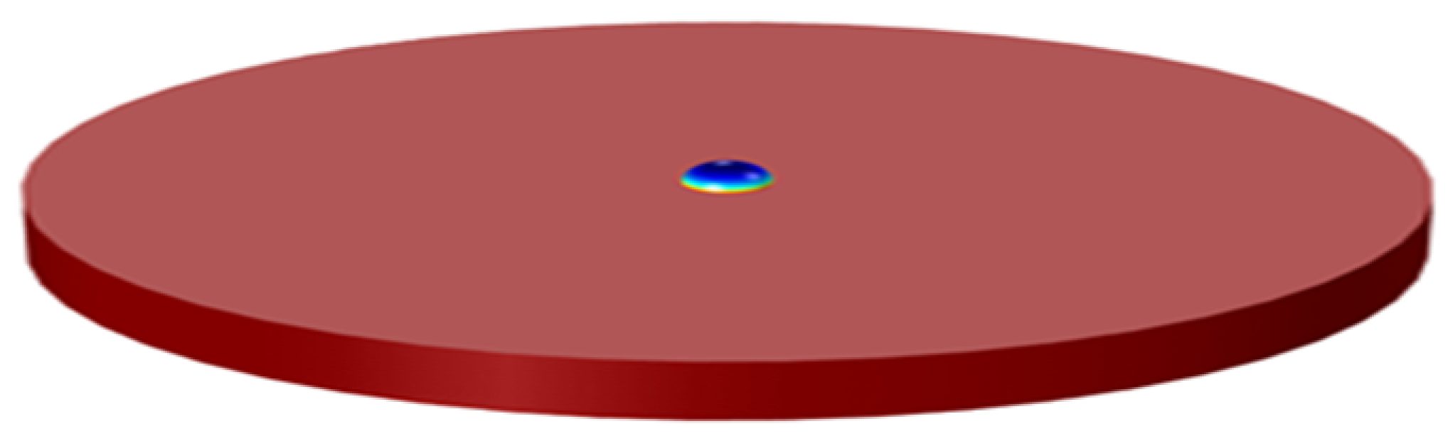
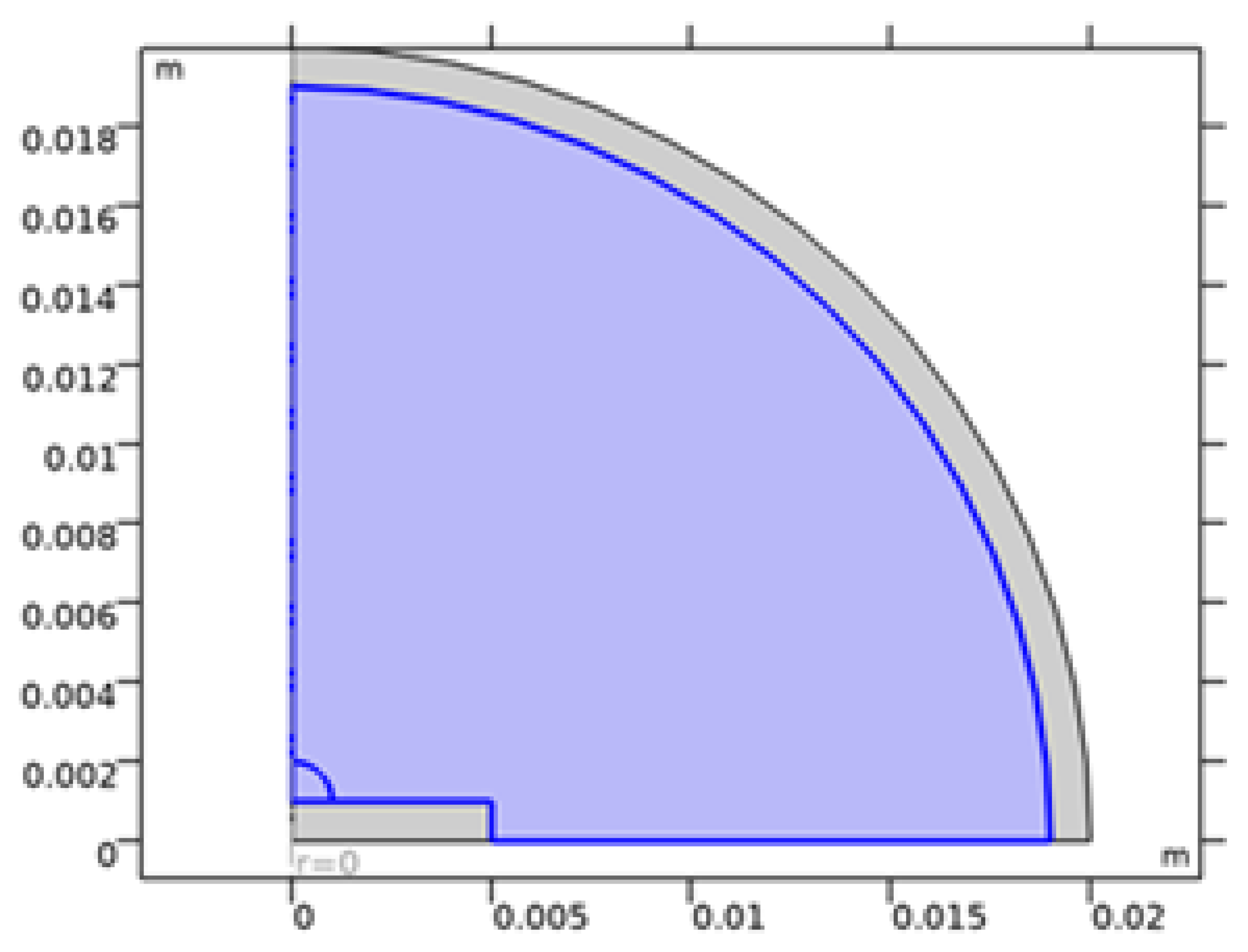
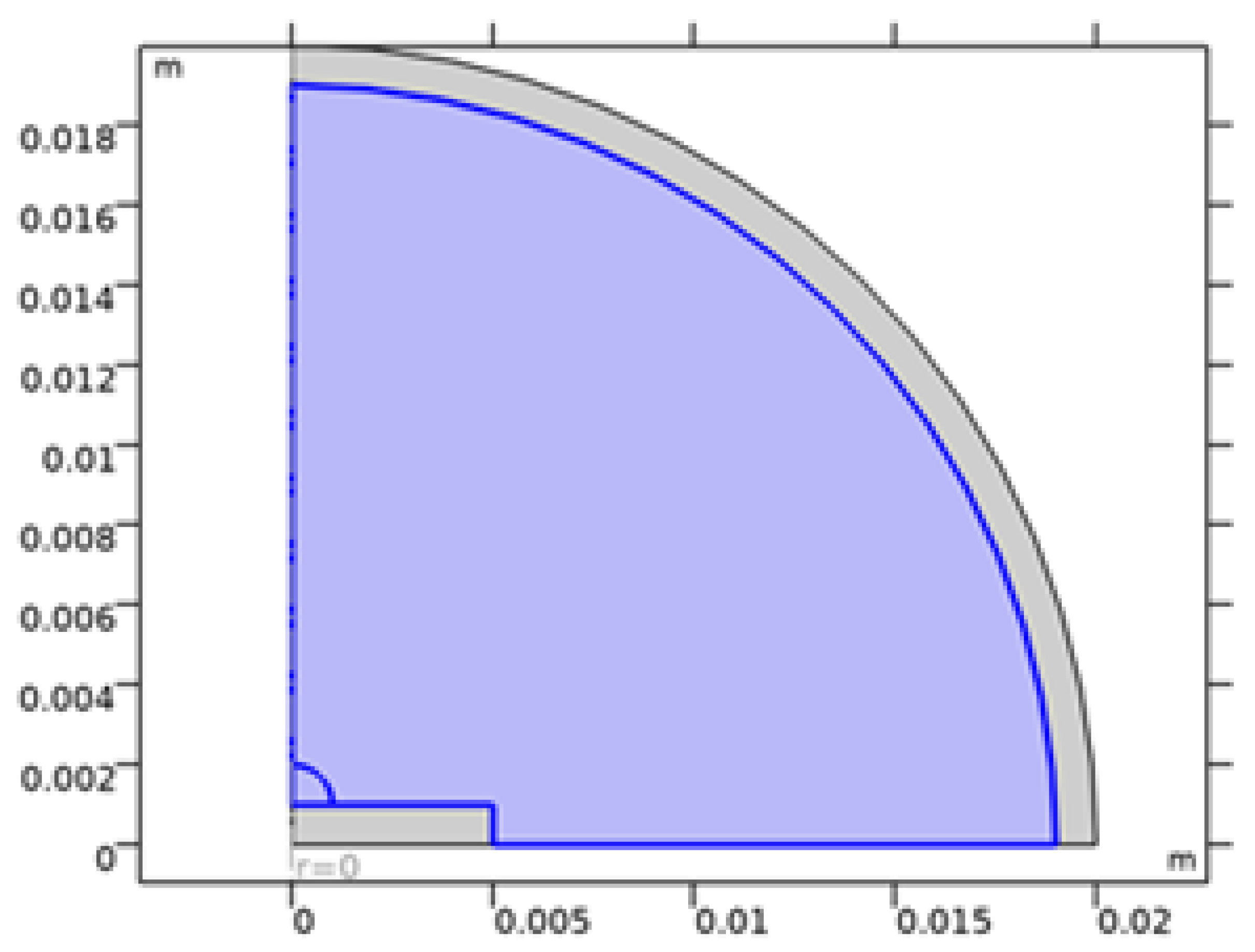
2.1. Geometry and Physical Setting

The computational domain consists of an initially spherical-cap sessile droplet of reactive silver ink placed on a structured silicon substrate with patterned wettability. The radial and axial coordinates are defined in an axisymmetric $(r,z)$ plane, as illustrated in Figure 2 and Figure 3 [2,6].

Figure 2 presents the overall axisymmetric domain. The droplet occupies a spherical-cap shaped region above the solid substrate, and the free surface is represented by a curved interface separating liquid and gas. The substrate thickness, radial extent, and domain boundaries are chosen large enough so that boundary conditions do not artificially influence the droplet-scale behavior [11,12].

Figure 3 zooms into the droplet region and highlights the contact-line area where the liquid, solid, and gas meet. This near-contact-line region is important because very steep temperature, concentration, and velocity gradients often occur there, and the evaporative flux can become strongly peaked close to the contact line [1,6].

Droplets with different initial volumes (approximately 5.2, 3.2, and $2.2$ $\mathsf{\mu }$$\mathrm{L}$) are deposited on heated substrates, which allows exploration of the role of droplet size on evaporation time and internal flow structures [9,12,19]. The time evolution of contact angle, footprint radius, and droplet height is measured using digital microscopy and is used both to guide model inputs and to compare overall evaporation trends [10,21].

Contact-line pinning and hysteresis strongly affect how the droplet footprint evolves during drying. Figure 4 schematically shows the advancing and receding contact angles, which define the range over which the contact line remains pinned even as the droplet shape changes [19,21]. When the actual contact angle remains between the advancing and receding limits, the footprint radius stays fixed and the contact angle decreases. Once the contact angle becomes smaller than the receding angle, the contact line can move inward and the footprint shrinks [2,12].

2.2. Governing Equations

The internal flow of the incompressible binary solvent (water/ethylene glycol) is described by the continuity and Navier–Stokes equations, coupled to energy and species transport [3,6].

Continuity (incompressible):

$$\nabla ·\mathbf{u}=0$$

(1)

Momentum (Navier–Stokes):

$$\rho \left({\displaystyle \frac{\partial \mathbf{u}}{\partial t}}+\mathbf{u}·\nabla \mathbf{u}\right)=-\nabla p+\mu {\nabla }^2\mathbf{u}+\rho \mathbf{g}$$

(2)

Energy (heat transfer in liquid):

$$\rho c_p\left({\displaystyle \frac{\partial T}{\partial t}}+\mathbf{u}·\nabla T\right)=k{\nabla }^{2}T$$

(3)

Species transport (binary solvent + solute):

$${\displaystyle \frac{\partial Y_i}{\partial t}}+\mathbf{u}·\nabla Y_i=\nabla ·\left(D_i\nabla Y_i\right)$$

(4)

Here, $\mathbf{u}=(u_r,u_z)$ is the fluid velocity vector, p is pressure, $\rho$ is density, $\mu$ is dynamic viscosity, $\mathbf{g}$ is gravity, T is temperature, $c_p$ is specific heat capacity, k is thermal conductivity, $Y_i$ is the mass fraction of species i, and $D_i$ is its diffusion coefficient [1,3,11]. These equations are solved in both the liquid and, where appropriate, in the solid substrate for heat conduction.

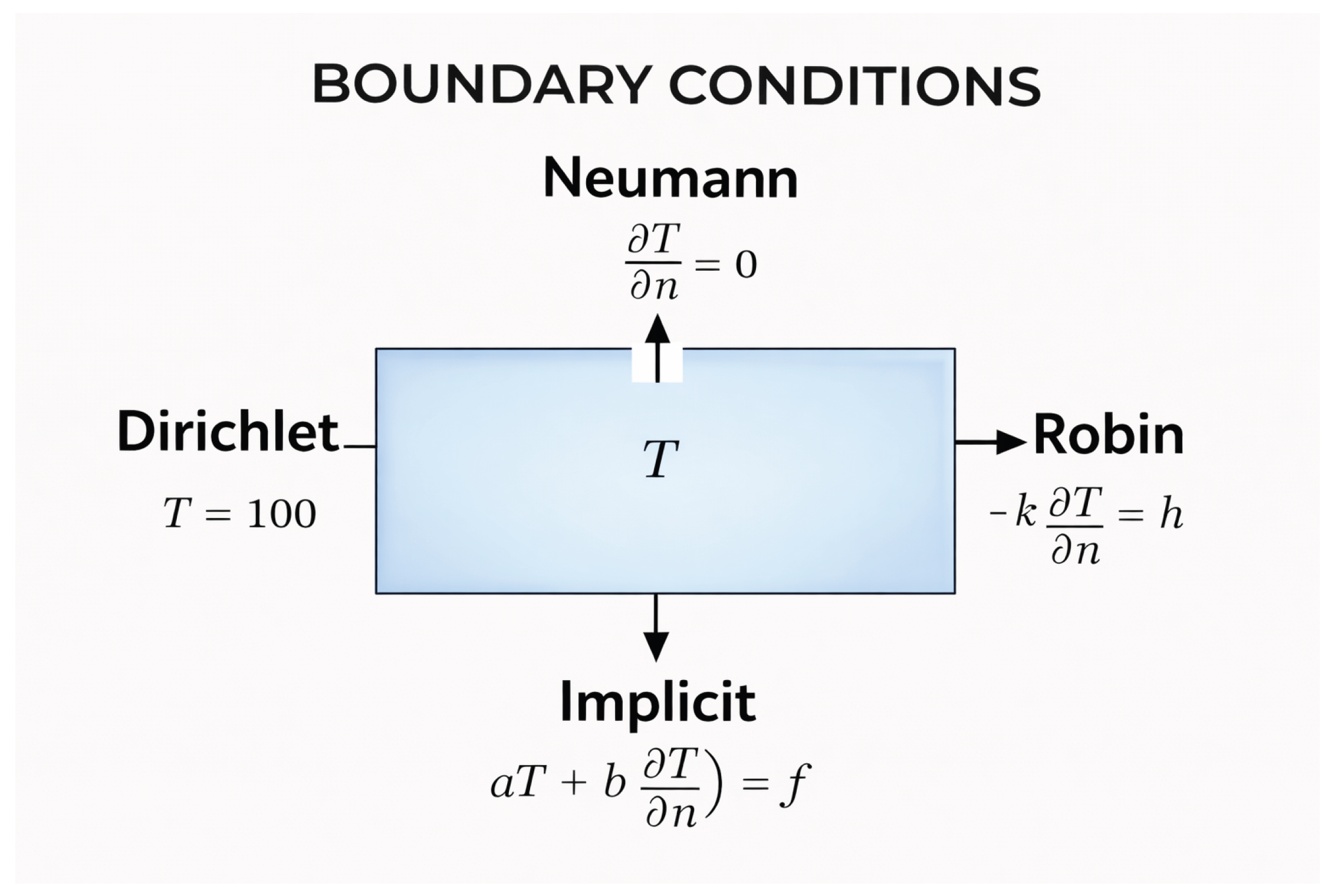
2.3. Marangoni Stresses at the Liquid–Gas Interface

Surface tension at the interface depends on both temperature and local composition of the more and less volatile components [4,7,21]. A linearized dependence is used:

$$\sigma ={\sigma }_0+\left({\displaystyle \frac{\partial \sigma }{\partial T}}\right)(T-T_0)+\left({\displaystyle \frac{\partial \sigma }{\partial Y}}\right)(Y_s-Y_0)$$

(5)

where ${\sigma }_0$ is the reference surface tension at $(T_0,Y_0)$, and $Y_s$ is the local interfacial mass fraction.

The tangential stress balance (Marangoni condition) along the free surface is

$$\mathbf{t}·\left(\tau ·\mathbf{n}\right)={\displaystyle \frac{\partial \sigma }{\partial s}}$$

(6)

with

$$\tau =\mu \left[\nabla \mathbf{u}+{(\nabla \mathbf{u})}^T\right],{\displaystyle \frac{\partial \sigma }{\partial s}}=\left({\displaystyle \frac{\partial \sigma }{\partial T}}\right){\displaystyle \frac{\partial T}{\partial s}}+\left({\displaystyle \frac{\partial \sigma }{\partial Y}}\right){\displaystyle \frac{\partial Y_s}{\partial s}}.$$

(7)

This formulation separates the contributions of thermal and compositional inhomogeneities to the Marangoni driving force, which is important in multicomponent droplets where both temperature and concentration vary along the surface [6,7,20].

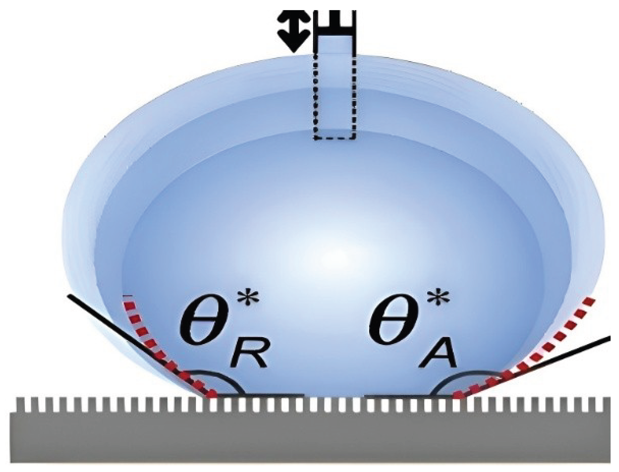
2.4. Boundary Conditions and Contact-Line Treatment

At the droplet–gas interface, standard Robin-type conditions are used for heat and mass transfer to represent exchange with the surrounding air [1,8,18]. The evaporative mass flux is related to the difference between the interfacial vapor concentration and the ambient value, and the associated latent heat is included as an energy sink in the liquid energy equation [3,18].

At the droplet–solid interface, continuity of temperature and heat flux is enforced between the droplet and the substrate, so that heat can conduct from the heated solid into the cooling liquid [11,12]. No-slip velocity conditions are applied at the solid surface, while appropriate symmetry conditions are used along the axis of rotation.

Figure 5 summarizes the main types of boundary conditions used in the model. Dirichlet conditions prescribe a variable (such as fixed temperature), Neumann conditions prescribe its normal gradient or flux, and Robin conditions combine both effects, often representing convective or radiative exchange with an environment [1,19].

Near the three-phase contact line, classical continuum models predict singular evaporative fluxes and very large velocity gradients. Several regularization strategies have been proposed in the literature, such as introducing a microscale cut-off, using slip models, or smoothing the contact-angle evolution [6,18,19]. In the present work, a smooth step function is used to transition between different evaporation or wetting regimes and to preserve numerical stability (see Section 4.4).

Table 1 summarizes representative parameters used in the simulations, including diffusion coefficients, latent heat, surface tension, and reference temperatures. These values are consistent with commonly reported data for water and water-based mixtures under ambient conditions [1,8,21].

3. Numerical Implementation

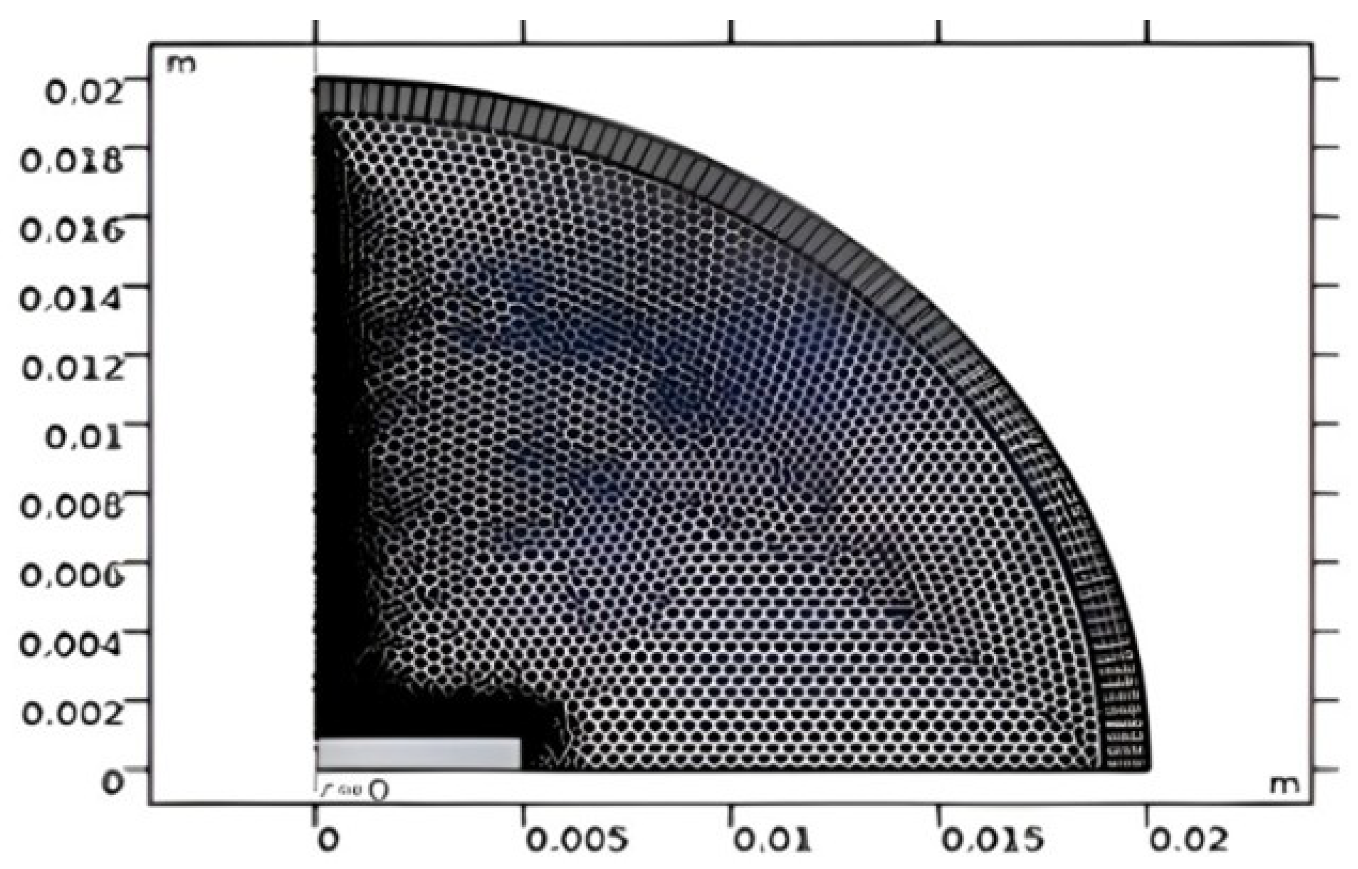
3.1. Meshing and Time Integration

The computational domain is discretized using finite elements with strong refinement near the contact line and free surface to resolve steep gradients. Figure 6 shows a representative mesh used for the axisymmetric droplet problem [3,6].

In Figure 6, small elements follow the curved liquid–gas interface and cluster near the contact line. This mesh design enables accurate resolution of near-singular evaporative fluxes while keeping the number of elements manageable. Coarser elements are used in regions farther from the droplet where gradients are weaker, especially deep in the solid substrate [11,12].

Time integration is carried out with an implicit solver that can adapt the time step based on estimated error and convergence behavior. Smaller time steps are usually required at early times, when the geometry and fields change rapidly, and at later times when the droplet becomes very thin and the free-surface motion accelerates [3,21]

3.2. Moving Mesh and Free-Surface Tracking

The evolution of the liquid–gas interface is captured using an ALE moving mesh formulation [3,6]. In this approach, the mesh nodes move with the interface, and the governing equations are solved in a deforming coordinate system while maintaining mesh quality.

Figure 7 shows a three-dimensional rendering of the droplet-on-substrate configuration used for visualization. Although the underlying computation is axisymmetric, this 3D view helps to visualize the droplet shape and to map scalar fields (such as temperature) onto the surface in a more intuitive way [6,7].

The ALE method avoids numerical diffusion of the interface that is sometimes seen in fixed-grid approaches such as volume-of-fluid or level-set, at the cost of some additional complexity in handling large deformations and possible mesh tangling. In the present simulations, moderate mesh smoothing and occasional remeshing are sufficient to maintain good element quality throughout the droplet lifetime [3,21].

4. Results and Discussion

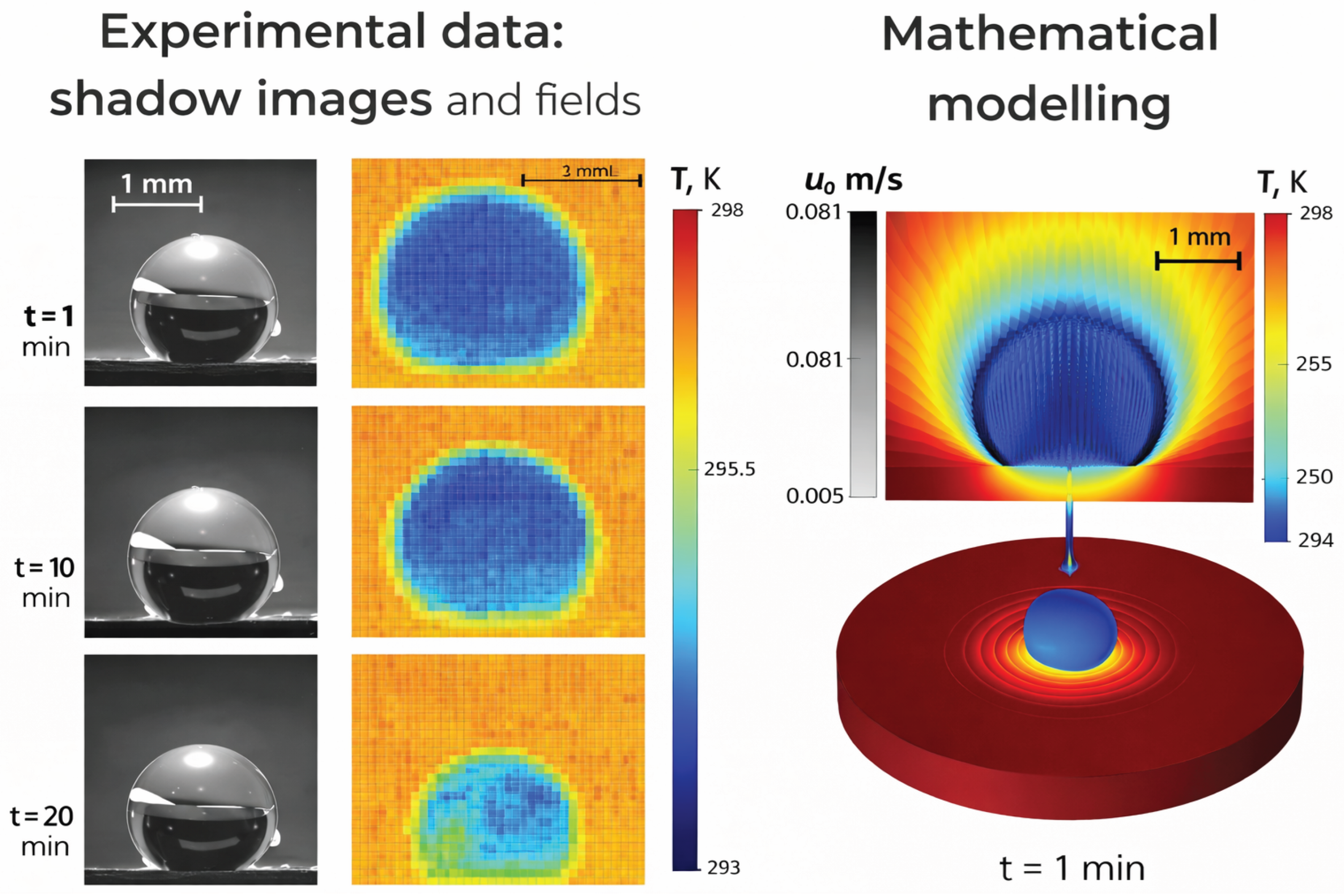
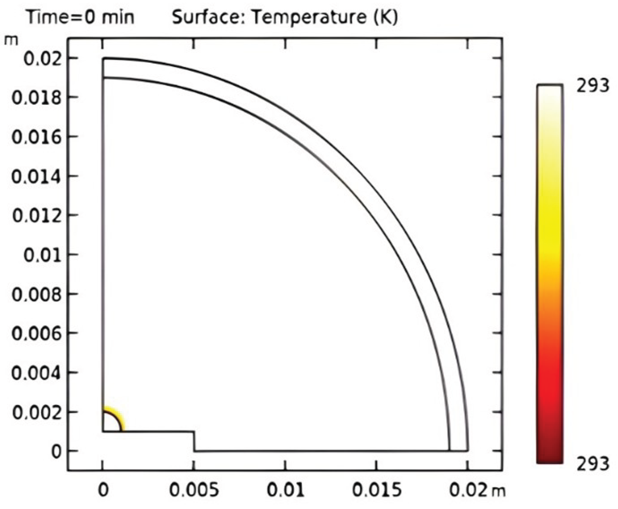
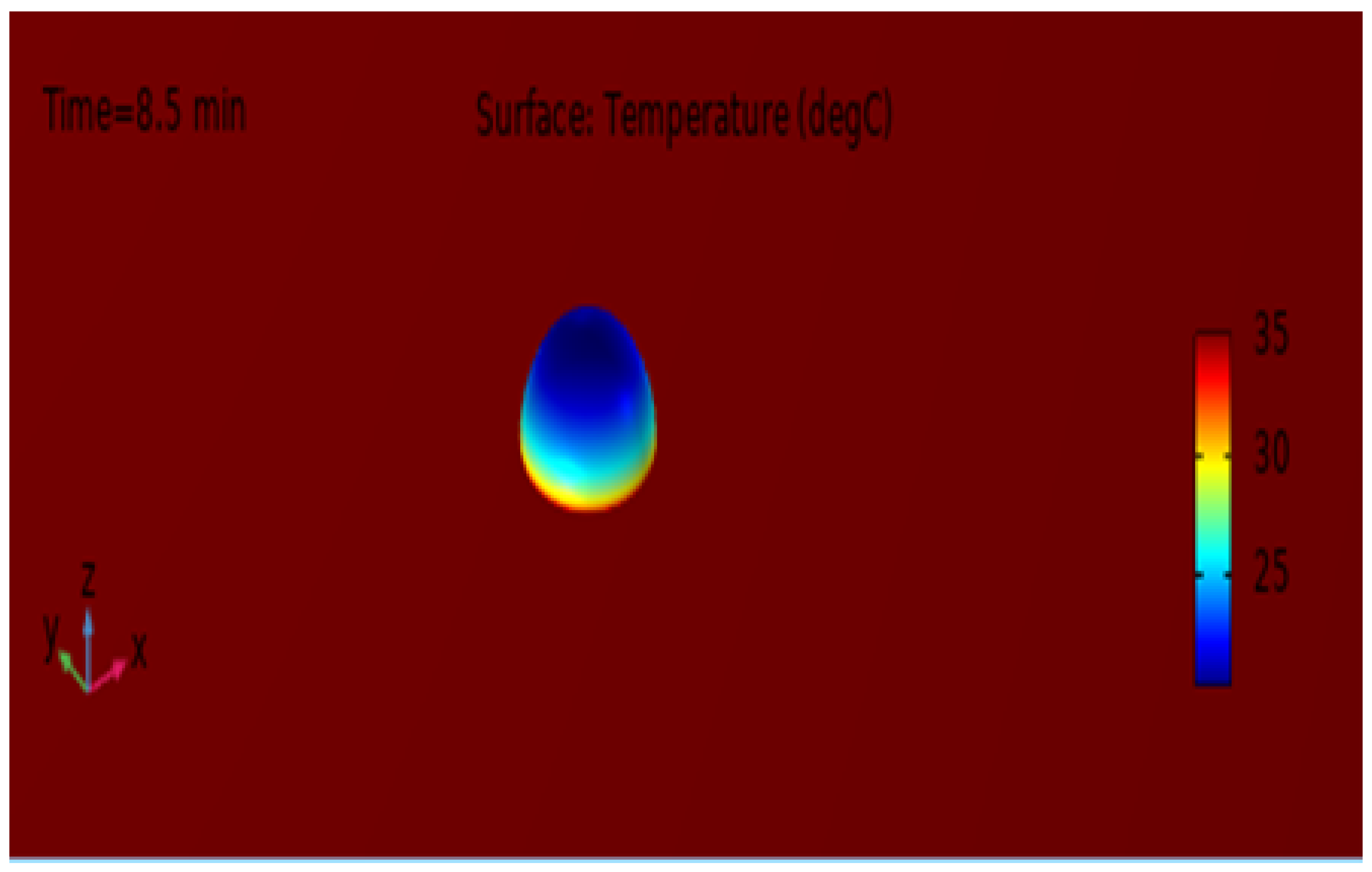
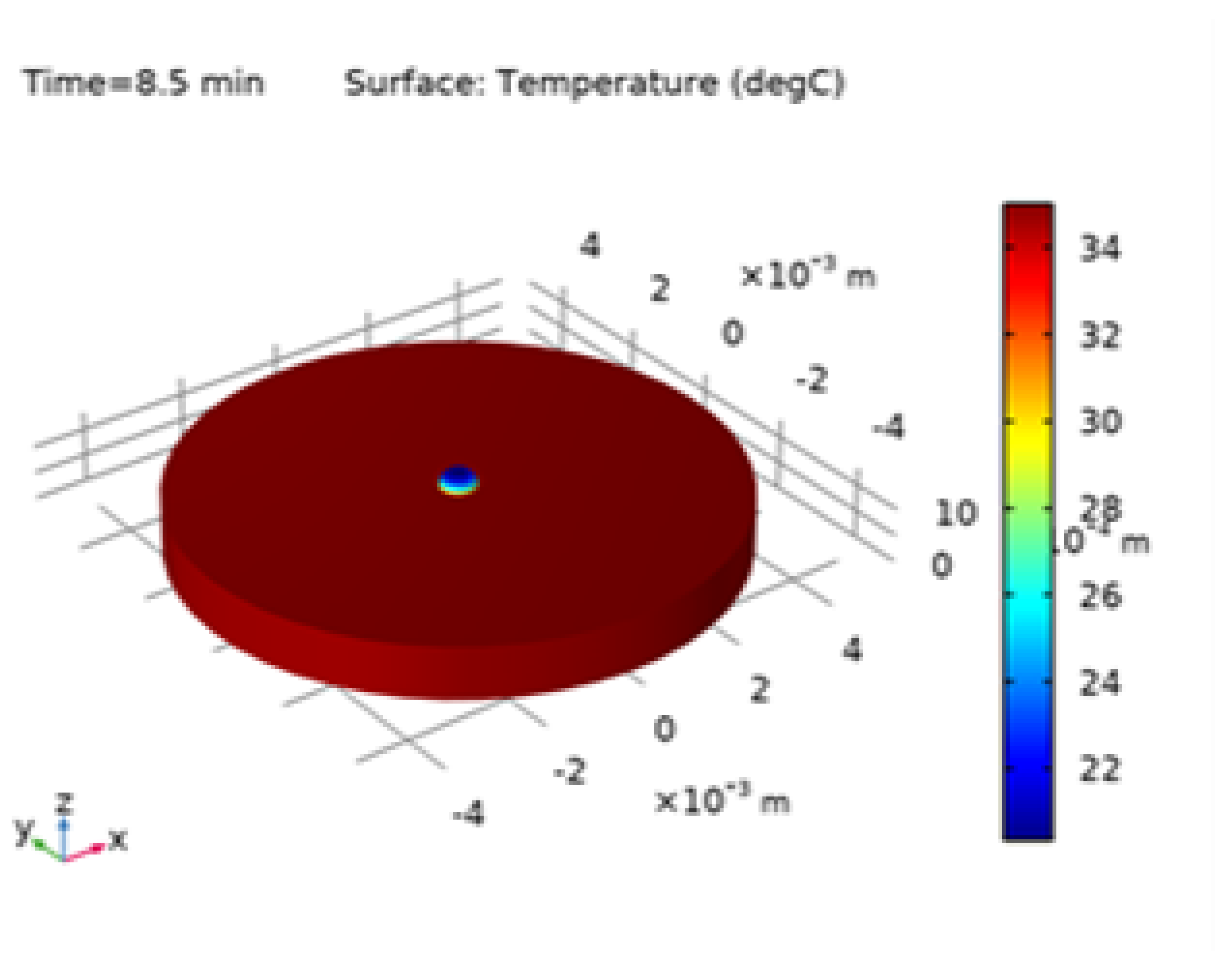
4.1. Initial and Surface Thermal Fields

The simulations are initialized close to an isothermal reference state. Figure 8 shows the initial surface temperature distribution at $t=0$ min for the isothermal case. As expected, the droplet surface and the exposed substrate have a nearly uniform temperature equal to the reference value, confirming that the initial and boundary conditions are applied consistently [1,11].

As evaporation progresses under heating, strong surface temperature gradients develop. Figure 9 presents the droplet surface temperature at $t=8.5$ min, where evaporative cooling produces lower temperatures near the upper free surface, while conductive heating from the substrate sustains higher temperatures near the base region [3,12].

Figure 10 and Figure 11 show independent three-dimensional renderings of the same temperature field at $t=8.5$ min using slightly different visualization settings. These figures demonstrate both the magnitude of the thermal gradients and the robustness of the post-processing routines, since the underlying numerical data produce consistent thermal patterns [6,10].

These temperature gradients along the free surface directly drive thermal Marangoni flows through the surface-tension dependence on temperature in Equation (5). The hotter region near the contact line typically has lower surface tension, while the cooler region near the droplet apex has higher surface tension, leading to surface flows that can significantly modify internal circulation [4,7,20].

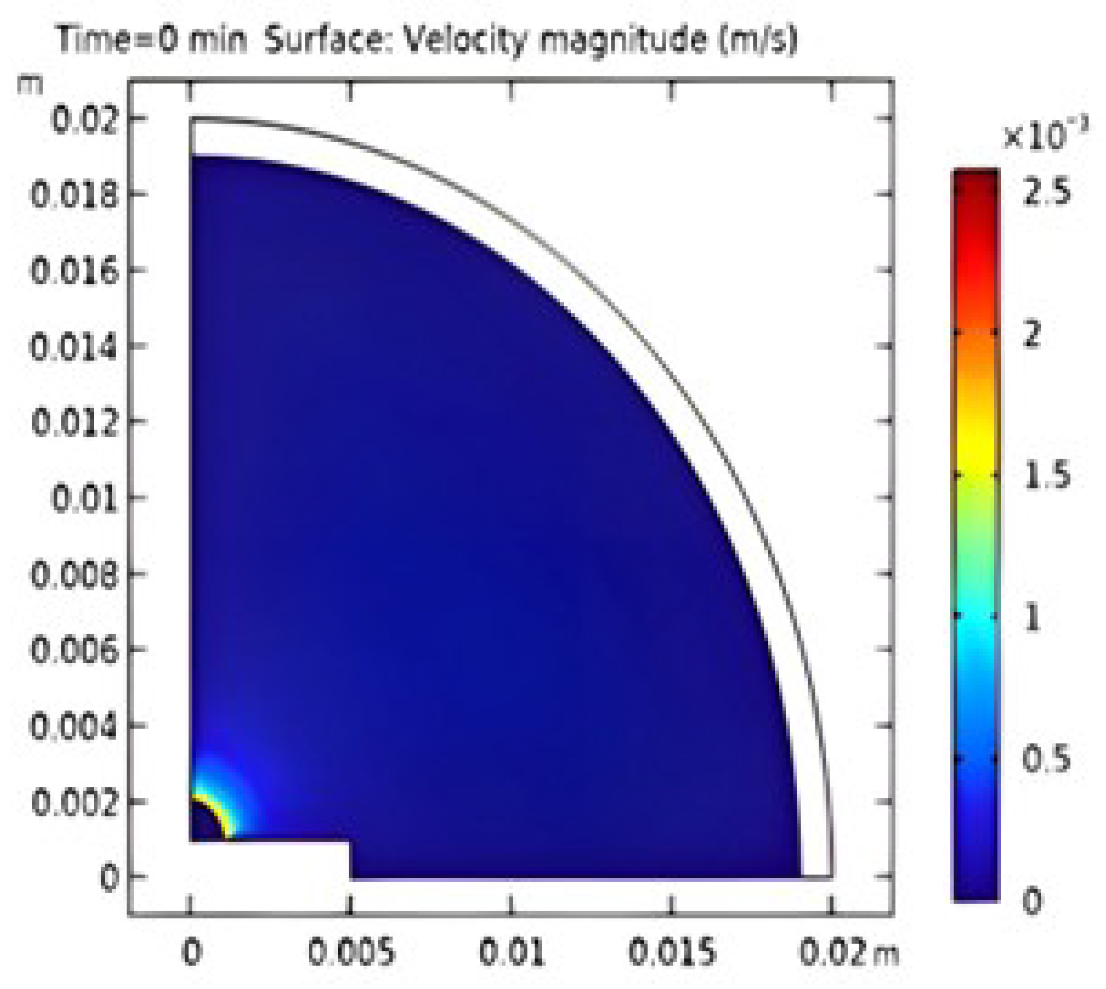
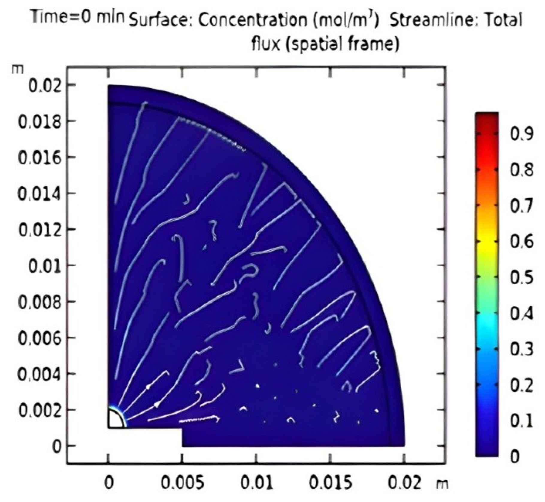
4.2. Flow and Transport Fields

The predicted early-time surface velocity magnitude and solute transport patterns are shown in Figure 12 and Figure 13, respectively [3,6].

Figure 12 displays the surface velocity magnitude at $t=0$ min in the axisymmetric domain. Even at this early stage, the largest velocities occur near the contact-line region, which is consistent with the strong shear and recirculation that often develop where the evaporative flux is highest [6,18]. The velocity field suggests that fluid is drawn along the surface from lower-flux regions toward the edge, where it then turns inward below the surface, creating a recirculation cell.

Figure 13 shows the surface concentration field at $t=0$ min together with total-flux streamlines in the spatial frame. These streamlines represent the combined effect of advection and diffusion on solute transport. They highlight the transport pathways that redistribute solute within the droplet during early evaporation and indicate how particles can be swept toward or away from the contact line depending on the direction and strength of the internal flow [3,7].

These flow and transport features are essential for understanding how silver particles move and eventually deposit on the substrate. Under suitable heating and solvent composition, thermocapillary flows can oppose the purely capillary-driven coffee-ring circulation and promote a more uniform final deposit [5,20,21].

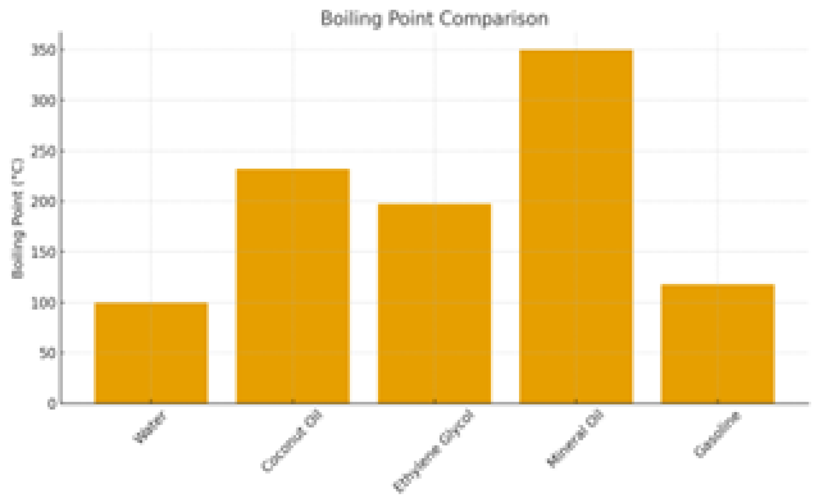
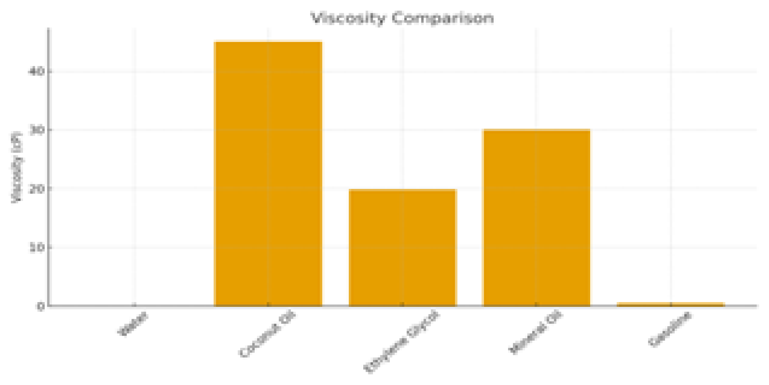
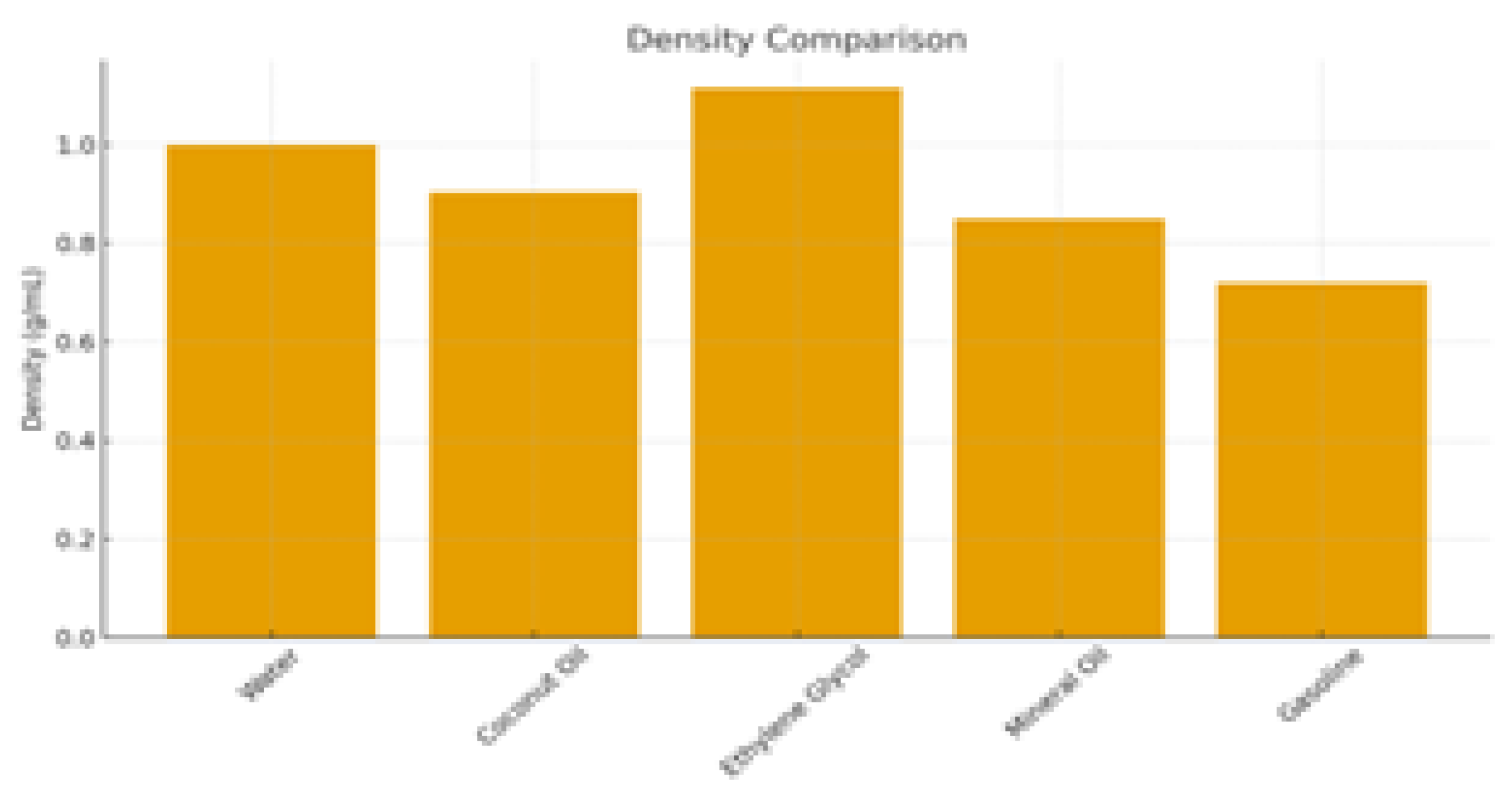
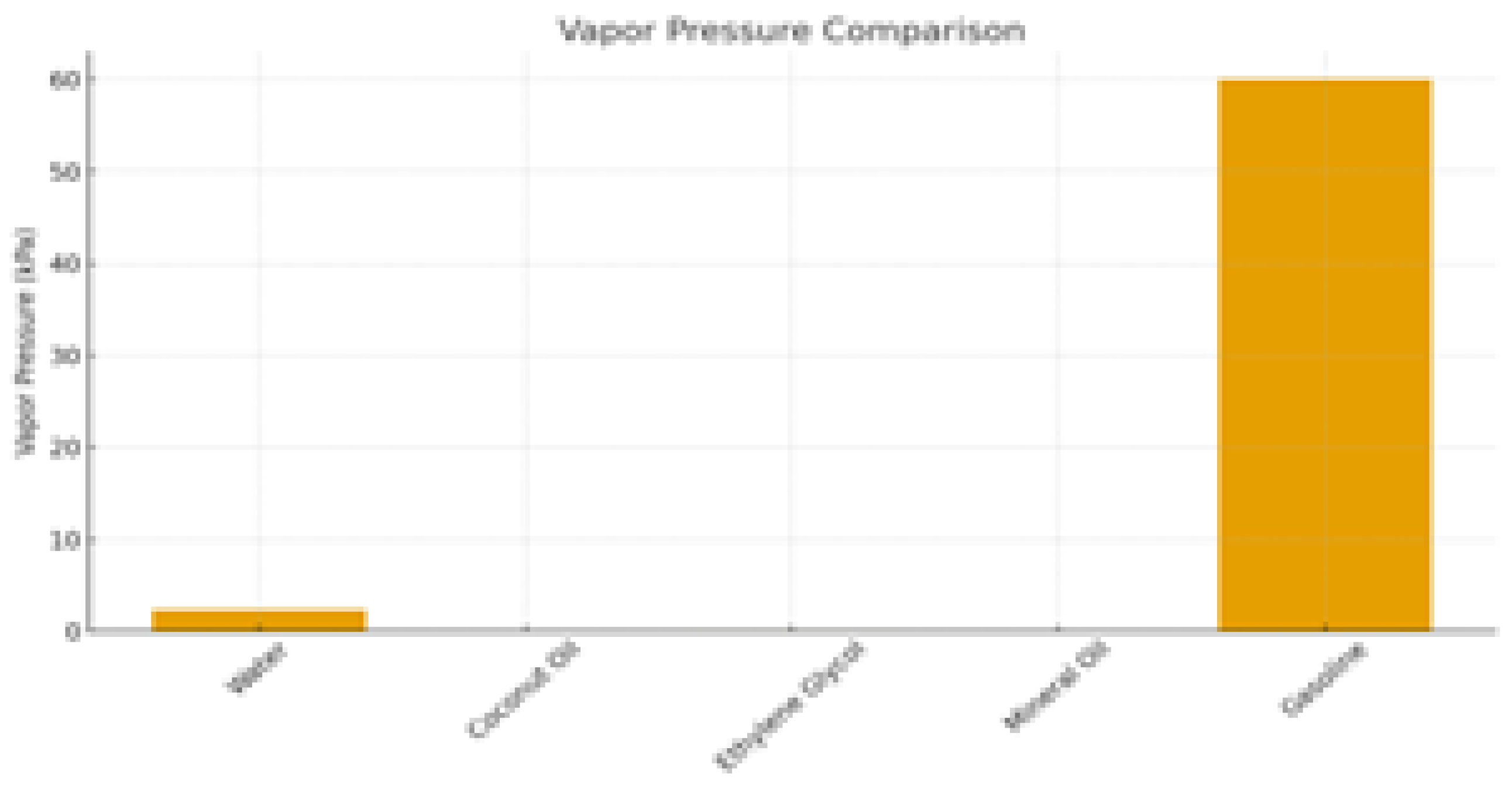
4.3. Comparison of Liquid Properties

To contextualize evaporation behavior for different fluids, representative property comparisons are provided in Figure 14, Figure 15, Figure 16 and Figure 17 and in Table 2. These data emphasize that volatility, viscosity, and surface tension can vary by orders of magnitude between liquids and therefore strongly affect droplet lifetimes and internal flows [1,21].

Figure 14 compares normal boiling points for several representative liquids commonly used in evaporation studies. Water, ethylene glycol, oils, and gasoline cover a broad range of boiling temperatures, and this correlates with their relative volatility under ambient conditions [1,21].

Figure 15 shows dynamic viscosities for the same set of liquids. Large viscosity contrasts strongly influence internal flow resistance and Marangoni circulation strength: for example, highly viscous ethylene glycol or oils produce slower, more damped flows than low-viscosity liquids such as water or gasoline [7,22].

Figure 16 compares densities of the same liquids. Although density variations are modest compared to differences in viscosity and vapor pressure, they still impact gravitational deformation of droplets and can slightly modify hydrostatic pressure distributions [2,11].

Finally, Figure 17 compares vapor pressures at ambient conditions. Gasoline exhibits relatively high vapor pressure, while water and ethylene glycol have moderate and very low vapor pressures, respectively. These contrasts highlight the dominant role of volatility in controlling evaporation rates [1,8].

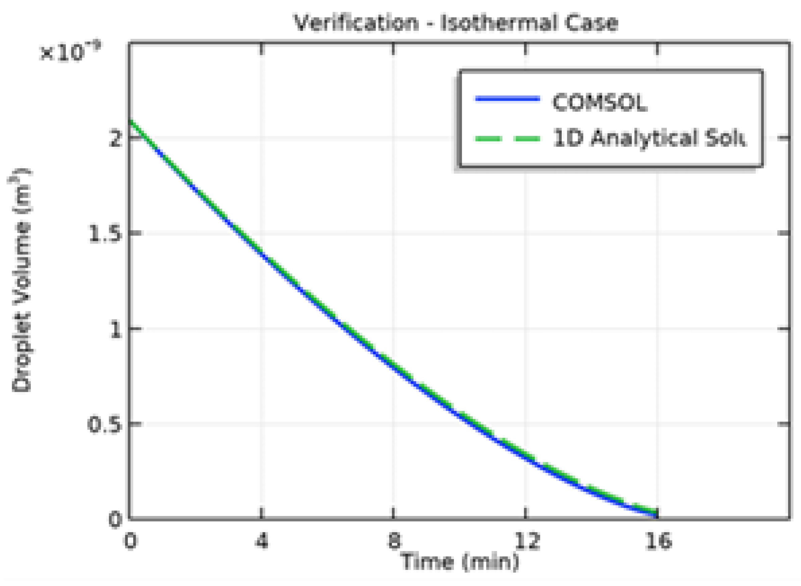
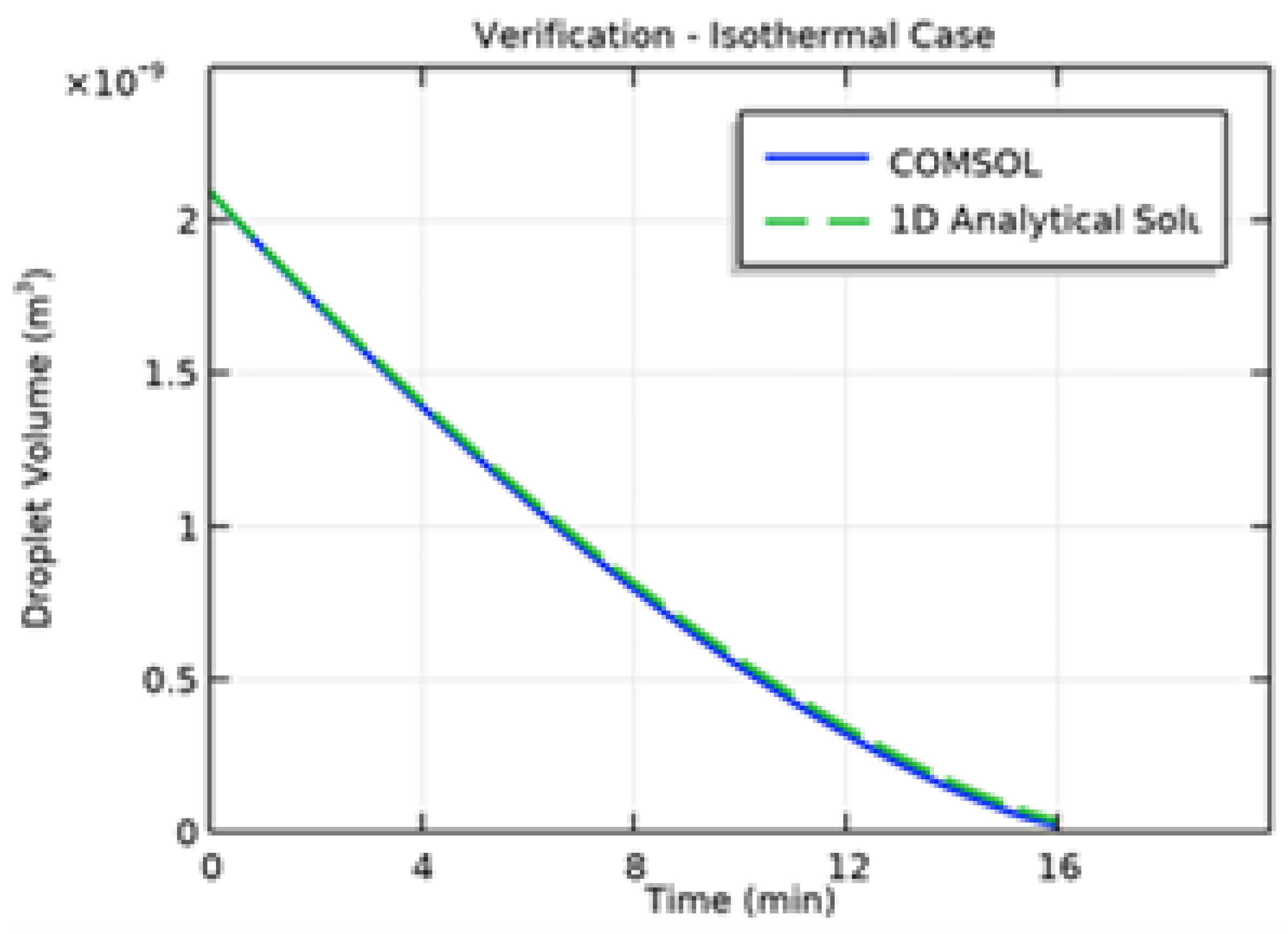
4.4. Model Verification and Numerical Regularization

An axisymmetric geometry used for model verification is shown in Figure 18. This simple spherical-cap shape allows direct comparison between the COMSOL simulations and analytical or semi-analytical solutions for diffusion-limited evaporation [2,6,8].

Figure 19 compares the evolution of droplet volume under isothermal conditions predicted by COMSOL with a 1D analytical solution. The agreement is excellent throughout the drying process, which confirms that the chosen mesh, time-stepping strategy, and boundary conditions accurately capture diffusion-limited evaporation in the absence of strong temperature gradients [2,8,18].

To maintain numerical stability when switching between different evaporation regimes or contact-line behaviors, a smooth step function is introduced. Figure 20 and Figure 21 illustrate this function, which provides a gradual transition rather than an abrupt change in model parameters or boundary conditions [6,19].

Figure 22 and Figure 23 show additional verification plots for the isothermal case using the same axisymmetric droplet geometry. Figure 22 emphasizes that the same geometric assumptions are used in both isothermal and non-isothermal simulations, ensuring that differences in results truly arise from thermal effects rather than geometry changes [11,12].

Figure 23 independently reproduces the comparison of droplet volume decay between COMSOL and the analytical solution. This reinforces the robustness of the numerical implementation and shows that the verification results are repeatable [2,8].

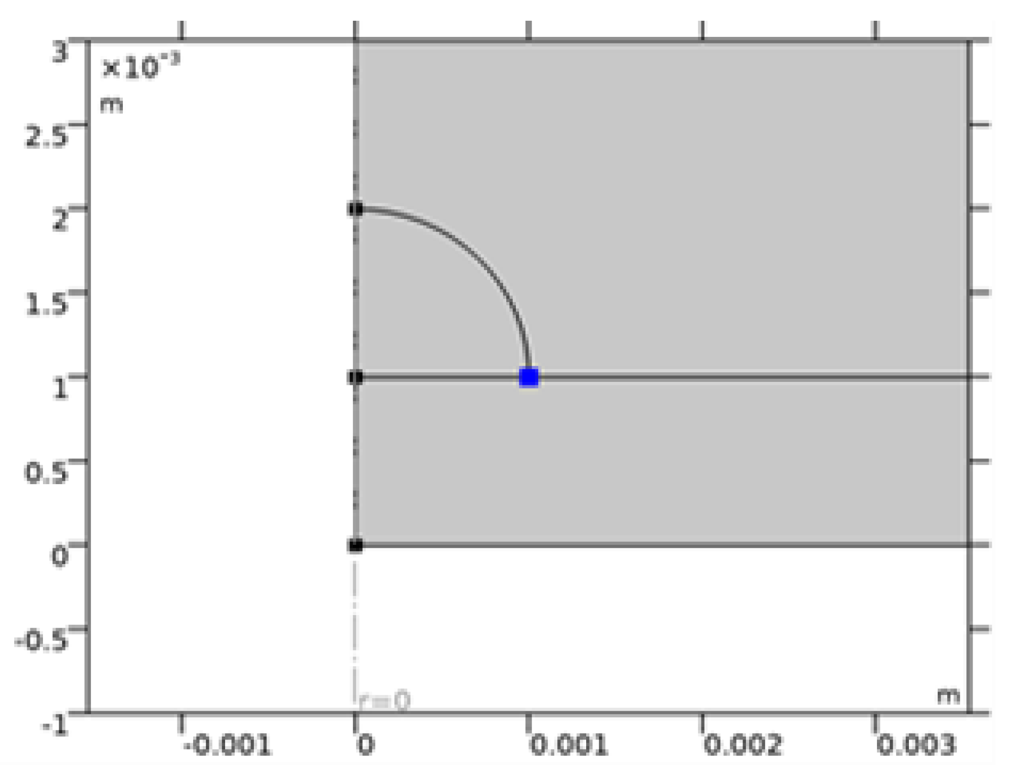
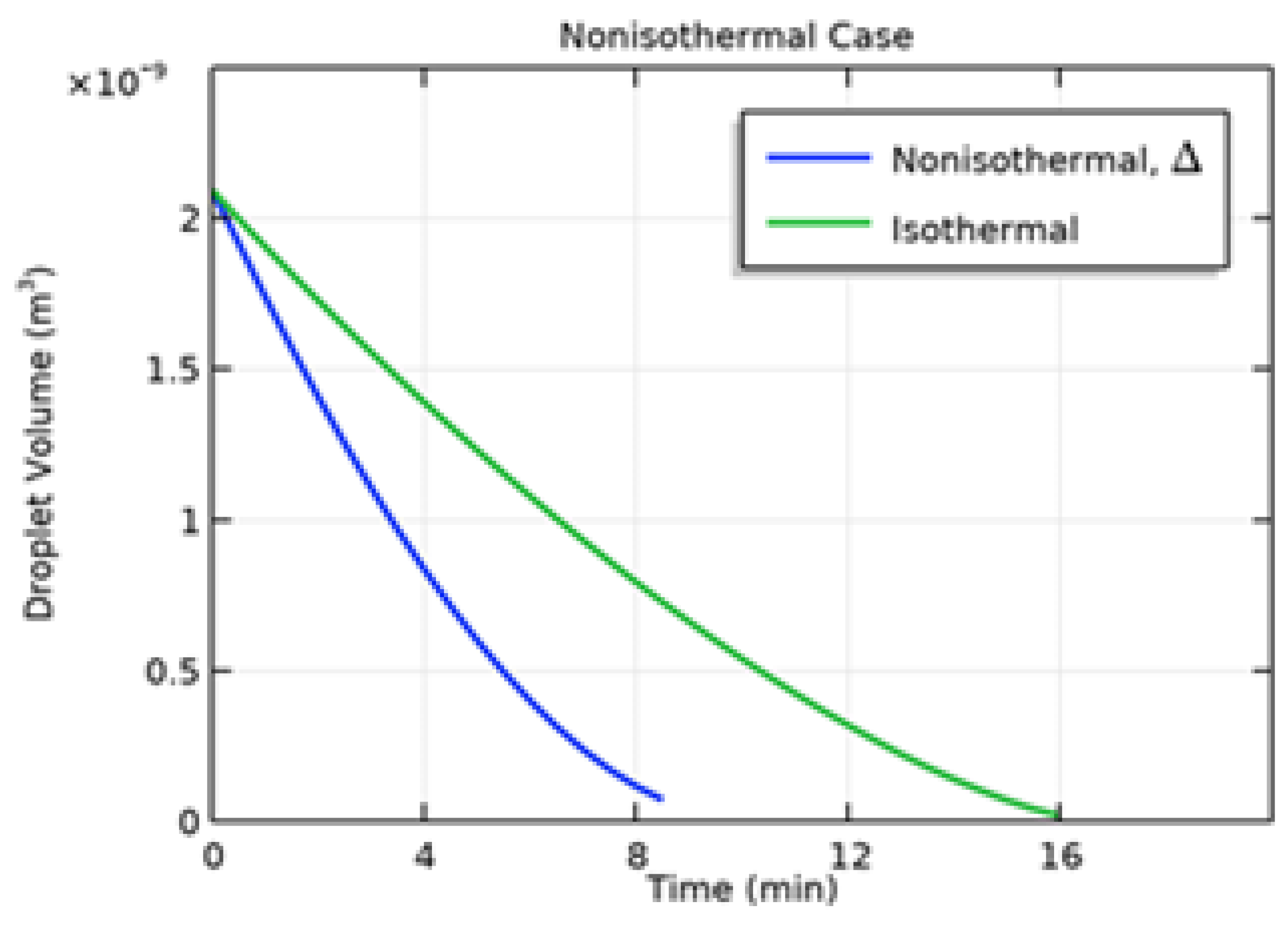
4.5. Additional Geometry and Isothermal vs Non-isothermal Comparison

Figure 24 and Figure 25 highlight the axisymmetric geometry and near-contact-line region used for coupled droplet–substrate simulations under non-isothermal conditions [11,12]. These figures make clear that the substrate thickness and lateral extent are sufficient to capture important heat-conduction effects and that the near-contact-line mesh is refined to resolve steep gradients.

Figure 26 and Figure 27 compare droplet volume decay for isothermal and non-isothermal evaporation. In Figure 26, non-isothermal conditions lead to faster evaporation than the purely isothermal case because the heated substrate supplies additional energy to the liquid and enhances temperature gradients that drive thermocapillary flows [1,12].

Figure 27 reproduces the same comparison but with an independently generated dataset or visualization. The two curves again show that thermal effects systematically shorten the drying time and can modify the relative importance of different evaporation modes (constant radius versus constant angle) [2,18].

5. Conclusions

A computational framework has been developed to study coupled heat, mass, and momentum transport in evaporating sessile droplets relevant to printed electronics. Experimental and model agreement for temperature fields is demonstrated in Figure 1, where the simulated temperature distribution closely matches infrared measurements for a heated droplet [4,21].

Strong surface temperature gradients (Figure 9, Figure 10 and Figure 11) and complex flow/transport features (Figure 12 and Figure 13) highlight the importance of resolving non-isothermal and composition-driven Marangoni effects to predict particle redistribution and final deposit morphology [3,7,20]. Verification against an analytical solution (Figure 19) supports the numerical implementation, while regularization strategies based on smooth step functions (Figure 20 and Figure 21) improve robustness and convergence [8,19].

Comparisons of isothermal versus non-isothermal evaporation (Figure 26 and Figure 27) illustrate the systematic influence of thermal effects on drying time scales and internal circulation, which can be used to design process conditions that suppress the coffee-ring effect and promote uniform deposits [5,21]. The present framework thus provides a useful link between simple diffusion-limited models and more complete multiphysics simulations, and it can guide the optimization of ink formulations and substrate heating strategies in practical printed-electronics applications [1,4,20].

References

1. Al Qubeissi, M.; et al. Heating and Evaporation of Droplets of Multicomponent and Blended Fuels: A Review of Recent Modeling Approaches. Energy Fuels 2021, 35(22), 18220–18256. [Google Scholar] [CrossRef]
2. D’Ambrosio, H.-M.; Wilson, S. K.; Wray, A. W.; Duffy, B. R. Effect of gravity-induced shape change on the diffusion-limited evaporation of thin sessile and pendant droplets. Phys. Rev. E 2025, 111(4), 045107. [Google Scholar] [CrossRef] [PubMed]
3. Diddens, C.; Kuerten, J. G. M.; van der Geld, C. W. M.; Wijshoff, H. M. A. Modeling the evaporation of sessile multi-component droplets. J. Colloid Interface Sci. 2017, 487, 426–436. [Google Scholar] [CrossRef] [PubMed]
4. He, M.; Liao, D.; Qiu, H. Multicomponent Droplet Evaporation on Chemical Micro-Patterned Surfaces. Sci. Rep. 2017, 7, 41897. [Google Scholar] [CrossRef]
5. Li, Y.; et al. Evaporation-Triggered Segregation of Sessile Binary Droplets. Phys. Rev. Lett. 2018, 120(22), 224501. [Google Scholar] [CrossRef]
6. Sáenz, P. J.; Sefiane, K.; Kim, J.; Matar, O. K.; Valluri, P. Evaporation of sessile drops: a three-dimensional approach. J. Fluid Mech. 2015, 772, 705–739. [Google Scholar] [CrossRef]
7. Thayyil Raju, L.; et al. Evaporation of a Sessile Colloidal Water–Glycerol Droplet: Marangoni Ring Formation. Langmuir 2022, 38(39), 12082–12094. [Google Scholar] [CrossRef]
8. Widmann, J. F.; Davis, E. J. Evaporation of Multicomponent Droplets. Aerosol Sci. Technol. 1997, 27(2), 243–254. [Google Scholar] [CrossRef]
9. Antonov, D. V.; Fedorenko, R. M.; Strizhak, P. A.; Sazhin, S. S. A simple model of heating and evaporation of droplets on a superhydrophobic surface. Int. J. Heat Mass Transf. 2023, 201, 123568. [Google Scholar] [CrossRef]
10. Ozturk, T.; Erbil, H. Y. Evaporation of water-ethanol binary sessile drop on fluoropolymer surfaces: Influence of relative humidity. Colloids Surf. A 2018, 553, 327–336. [Google Scholar] [CrossRef]
11. Tonini, S.; Cossali, G. E. Modeling the evaporation of sessile drops deformed by gravity on hydrophilic and hydrophobic substrates. Phys. Fluids 2023, 35(3), 032113. [Google Scholar] [CrossRef]
12. Volkov, R. S.; Strizhak, P. A.; Misyura, S. Y.; Lezhnin, S. I.; Morozov, V. S. The influence of key factors on the heat and mass transfer of a sessile droplet. Exp. Therm. Fluid Sci. 2018, 99, 59–70. [Google Scholar] [CrossRef]
13. Hussain, M. A.; Yesudasan, S.; Chacko, S. Nanofluids for solar thermal collection and energy conversion. Preprints preprint article 2020. [Google Scholar]
14. Yesudasan, S. The critical diameter for continuous evaporation is between 3 and 4 nm for hydrophilic nanopores. Langmuir 2022, vol. 38(no. 21), 6550–6560. [Google Scholar] [CrossRef]
15. S. Yesudasan, “Thermal dynamics of heat pipes with sub-critical nanopores,” arXiv:2406.xxxxx [physics.flu-dyn], 2024, arXiv preprint.
16. M. M. Mohammed and S. Yesudasan, “Molecular dynamics study on the properties of liquid water in confined nanopores: Structural, transport, and thermodynamic insights,” in Proc. ASEE Northeast Section Conf., 2025, pp. 1–7. 1.
17. Hotchandani, V.; Mathew, B.; Yesudasan, S.; Chacko, S. Thermo-hydraulic characteristics of novel MEMS heat sink. Microsyst. Technol. 2021, vol. 27(no. 1), 145–157. [Google Scholar] [CrossRef]
18. Vlasov, V. A. Rigorous model of sessile droplet evaporation considering the kinetic factor. Phys. Rev. E 2025, 111(5), 055104. [Google Scholar] [CrossRef]
19. Shaikeea, A. J. D.; et al. Universal representations of evaporation modes in sessile droplets. PLOS ONE 2017, 12(9), e0184997. [Google Scholar] [CrossRef]
20. Rocha, D.; et al. Evaporating sessile droplets: solutal Marangoni effects overwhelm thermal Marangoni flow. arXiv 2024, arXiv:2410.17071. [Google Scholar] [CrossRef]
21. Wang, Z.; Orejon, D.; Takata, Y.; Sefiane, K. Wetting and evaporation of multicomponent droplets. Phys. Rep. 2022, 960, 1–37. [Google Scholar] [CrossRef]
22. Wang, Z.; et al. Surface properties and internal flows of evaporating multicomponent droplets. Curr. Opin. Colloid Interface Sci. 2022, 59, 101577. [Google Scholar] [CrossRef]
23. Picknett, R. G.; Bexon, R. The evaporation of sessile or pendant drops in still air. J. Colloid Interface Sci. 1977, 61(2), 336–350. [Google Scholar] [CrossRef]
24. Deegan, R. D.; et al. Capillary flow as the cause of ring stains from dried liquid drops. Nature 1997, 389, 827–829. [Google Scholar] [CrossRef]
25. Hu, H.; Larson, R. G. Evaporation of a sessile droplet on a substrate. J. Phys. Chem. B 2002, 106(6), 1334–1344. [Google Scholar] [CrossRef]
26. Cazabat, A.-M.; Guéna, G. Evaporation of macroscopic sessile droplets. Soft Matter 2010, 6, 2591–2612. [Google Scholar] [CrossRef]
27. Davidovitch, B.; Yerushalmi-Rozen, E.; Safran, A. Coating a substrate with an evaporating solution: A simple model. Phys. Rev. E 2005, 72(4), 041605. [Google Scholar] [CrossRef]
28. Erbil, H. Y. Evaporation of pure liquid sessile and spherical suspended drops: A review. Adv. Colloid Interface Sci. 2012, 170(1–2), 67–86. [Google Scholar] [CrossRef] [PubMed]
29. Bennacer, R.; Sefiane, K. Vapor diffusion versus liquid convection in evaporating sessile drops. J. Fluid Mech. 2014, 749, 649–665. [Google Scholar] [CrossRef]
30. Kim, H.; Lequeux, F.; Talini, L.; Allain, C. Dried colloidal suspensions on hydrophobic substrates: deposit morphology and cracking behavior. Soft Matter 2016, 12, 1547–1559. [Google Scholar] [CrossRef]
31. Yarin, A. L. Drop impact dynamics: Splashing, spreading, receding, bouncing. Annu. Rev. Fluid Mech. 2006, 38, 159–192. [Google Scholar] [CrossRef]
32. Sefiane, K. Patterns from drying drops. Adv. Colloid Interface Sci. 2014, 206, 372–381. [Google Scholar] [CrossRef] [PubMed]
33. Kim, H.; et al. Controlled uniform coating from the interplay of Marangoni flows and surface-adsorbed macromolecules. Phys. Rev. Lett. 2017, 119(18), 184501. [Google Scholar] [CrossRef]
34. Yakhno, T.; et al. Drying drops: deposit formation and patterning. Colloids Surf. A 2003, 231(1–3), 1–10. [Google Scholar] [CrossRef]
35. Bird, J. C.; de Ruiter, R. R.; Courbin, L.; Stone, H. A. Daughter droplet production from a kink in a soap film. Phys. Rev. Lett. 2009, 103(16), 164502. [Google Scholar] [CrossRef]
36. Sbragaglia, M.; et al. Slip and wettability of nanostructured surfaces. Phys. Rev. Lett. 2007, 99(15), 156001. [Google Scholar] [CrossRef] [PubMed]
37. Kavehpour, H. P. Coalescence of drops. Annu. Rev. Fluid Mech. 2015, 47, 245–268. [Google Scholar] [CrossRef]
38. Biance, A.-L.; Clanet, C.; Quéré, D. Evaporation of a sessile droplet. Langmuir 2003, 19(16), 6889–6894. [Google Scholar] [CrossRef]
39. McHale, G.; Newton, M. I. Global geometry and the equilibrium shapes of liquid drops on fibers. Colloids Surf. A 2009, 333(1–3), 38–47. [Google Scholar] [CrossRef]
40. Dash, S.; Garimella, M. R. Droplet evaporation dynamics on micropillar arrays. Langmuir 2014, 30(48), 14308–14315. [Google Scholar] [CrossRef]
41. Brutin, D.; Starov, V. Recent advances in droplet wetting and evaporation. Chem. Soc. Rev. 2018, 47, 558–585. [Google Scholar] [CrossRef]
42. Sobac, B.; Brutin, D. Thermal effects of the substrate on water droplet evaporation. Phys. Rev. E 2014, 90(5), 053011. [Google Scholar] [CrossRef] [PubMed]
43. Ruscher, M.; Lohse, D.; Diddens, C. Mixed-mode evaporation of binary liquid droplets. Phys. Rev. Fluids 2020, 5(7), 073602. [Google Scholar] [CrossRef]
44. Kumar, A.; et al. Drying of colloidal droplets on superhydrophobic surfaces: Suppression of the coffee-ring effect. Langmuir 2019, 35(31), 10212–10220. [Google Scholar] [CrossRef]
Figure 1. Comparison of experiment and simulation for a heated sessile droplet. Left: experimental shadow images and infrared-measured surface temperature fields at representative times. Right: corresponding mathematical/COMSOL prediction of the temperature field and droplet-on-substrate configuration (example shown at t = 1 min).
Preprints 191864 g001
Figure 2. Axisymmetric computational domain (rz plane) for a sessile droplet on a heated substrate. The liquid phase is modeled as a spherical-cap profile on a solid substrate region, with the free surface represented by the curved interface boundary.
Preprints 191864 g002
Figure 3. Zoomed view of the axisymmetric droplet geometry (mm scale). This view highlights the initial spherical-cap shape and the near-contact-line region where sharp thermal and solutal gradients can develop.
Preprints 191864 g003
Figure 4. Illustration of contact-angle hysteresis and contact-line pinning. The advancing θ A * and receding θ R * angles define the range over which the contact line remains pinned despite changes in droplet shape during evaporation.
Preprints 191864 g004
Figure 5. Schematic summary of standard boundary-condition types used in heat and mass transfer modeling: Dirichlet (prescribed field), Neumann (prescribed normal gradient or flux), Robin (mixed convective-type condition), and implicit linear combinations.
Preprints 191864 g005
Figure 6. Representative finite-element mesh for the axisymmetric droplet domain. The mesh is refined near the free surface and the contact-line region to capture strong local gradients and near-singular evaporative flux behavior.
Preprints 191864 g006
Figure 7. Three-dimensional rendering of the droplet-on-substrate configuration used for visualization of surface fields and global geometry (COMSOL view).
Preprints 191864 g007
Figure 8. Initial surface temperature distribution at t = 0 min under isothermal conditions ( T = 293 K ). The uniform temperature field confirms consistent initial and boundary conditions prior to evaporation-driven cooling.
Preprints 191864 g008
Figure 9. Droplet surface temperature field (°C) at t = 8.5 min. Evaporative cooling produces lower temperatures near the upper free surface, while conductive heating from the substrate sustains higher temperatures near the base region.
Preprints 191864 g009
Figure 10. Three-dimensional rendering of the droplet surface temperature field at t = 8.5 min, showing strong thermal gradients caused by evaporative cooling and substrate heating.
Preprints 191864 g010
Figure 11. Independent three-dimensional rendering of the droplet surface temperature field at t = 8.5 min, demonstrating consistency and repeatability of the thermal visualization.
Preprints 191864 g011
Figure 12. Surface velocity magnitude (m/s) at t = 0 min in the axisymmetric domain. The largest velocities occur near the contact-line region, consistent with strong near-surface shear and recirculation initiation.
Preprints 191864 g012
Figure 13. Surface concentration field ( mol/m 3 ) at t = 0 min with total-flux streamlines (spatial frame). Streamlines indicate the combined advective and diffusive transport pathways that redistribute solute within the droplet during early evaporation.
Preprints 191864 g013
Figure 14. Comparison of normal boiling points for representative liquids relevant to sessile droplet evaporation studies, illustrating wide differences in volatility.
Preprints 191864 g014
Figure 15. Comparison of dynamic viscosity for representative liquids. Large viscosity contrasts strongly influence internal flow resistance and Marangoni circulation strength.
Preprints 191864 g015
Figure 16. Density comparison of representative liquids commonly used in evaporation studies. Density variations are modest compared to differences in viscosity and vapor pressure.
Preprints 191864 g016
Figure 17. Comparison of vapor pressures at ambient conditions for representative liquids, highlighting the dominant role of volatility in controlling evaporation rates.
Preprints 191864 g017
Figure 18. Axisymmetric spherical-cap droplet geometry used for isothermal model verification, showing the computational domain and interface shape.
Preprints 191864 g018
Figure 19. Verification of the numerical model under isothermal conditions. Comparison of droplet volume decay predicted by COMSOL simulations and a 1D analytical solution shows excellent agreement.
Preprints 191864 g019
Figure 20. Smooth step function employed in the numerical implementation to enable gradual transitions between regimes while maintaining solver stability.
Preprints 191864 g020
Figure 21. Smooth step function used to introduce gradual transitions between regimes or boundary-condition states, improving numerical stability and solver convergence.
Preprints 191864 g021
Figure 22. Axisymmetric droplet geometry shown for consistency across verification and non-isothermal simulations, emphasizing identical geometric assumptions.
Preprints 191864 g022
Figure 23. Independent reproduction of the isothermal droplet volume decay comparison between COMSOL simulations and the analytical solution, confirming numerical robustness.
Preprints 191864 g023
Figure 24. Axisymmetric geometry of the coupled droplet–substrate system, highlighting the droplet footprint, contact-line location, and substrate thickness.
Preprints 191864 g024
Figure 25. Axisymmetric droplet geometry emphasizing the near-contact-line region, where steep gradients in temperature, velocity, and evaporative flux develop.
Preprints 191864 g025
Figure 26. Comparison of droplet volume decay for isothermal and non-isothermal evaporation. Non-isothermal conditions result in faster evaporation due to enhanced heat transfer and thermocapillary effects.
Preprints 191864 g026
Figure 27. Reproduction of the droplet volume decay comparison for isothermal and non-isothermal cases, confirming numerical robustness and the systematic influence of thermal effects.
Preprints 191864 g027