
Submitted:
27 December 2025
Posted:
29 December 2025
You are already at the latest version
Abstract
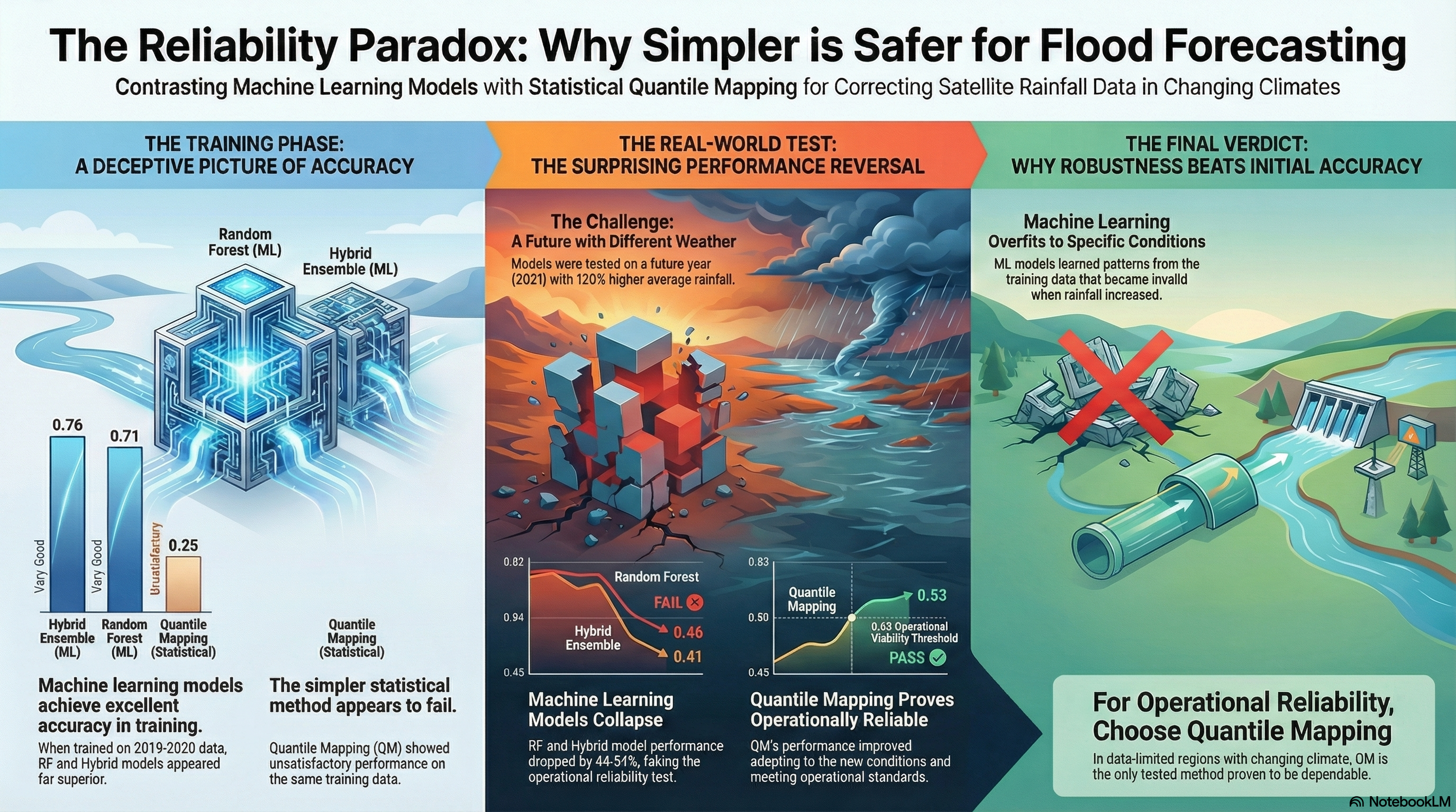
The Philippines experiences intense rainfall but has limited ground-based monitoring infrastructure for flood prediction. Satellite rainfall products provide broad coverage but contain systematic biases that reduce operational usefulness. This study evaluated three correction methods—Quantile Mapping (QM), Random Forest (RF), and Hybrid Ensemble—for improving Satellite Rainfall Monitor (SRM) estimates in the Cagayan de Oro River Basin, Northern Mindanao. When trained on comprehensive 2019-2020 data, Random Forest and Hybrid Ensemble substantially outperformed Quantile Map-ping, achieving excellent calibration accuracy (R² = 0.71 and 0.76 versus R² = 0.25 for QM). However, when tested on an independent year with substantially different rain-fall patterns (2021: 120% higher mean rainfall, 33% increase in rainy-day frequency), performance rankings reversed completely. Quantile Mapping maintained satisfactory operational performance (R² = 0.53, RMSE = 5.23 mm), showing improvement over training conditions, while Random Forest and Hybrid Ensemble both failed dramati-cally, with R² dropping to 0.46 and 0.41 respectively despite their excellent training performance. This highlights that training accuracy alone poorly predicts operational reliability under changing rainfall regimes. Quantile Mapping's percentile-based cor-rection naturally adapts when rainfall patterns shift without requiring recalibration, while machine learning methods learned magnitude-specific patterns that failed when conditions changed. For flood early warning in basins with limited data, equipment failures, and variable rainfall, only Quantile Mapping proved operationally reliable. This has practical implications for disaster risk reduction across the Philippines and similar tropical regions where standard validation approaches may systematically mislead model selection by measuring calibration performance rather than operational transferability.
Keywords:
satellite rainfall monitor
; quantile mapping
; random forest
; temporal transferability
; flood early warning
; Philippines
1. Introduction
Accurate rainfall information is essential for hydrological modeling and disaster risk reduction, yet many region lack dense and reliable ground-based monitoring networks [1,2]. Satellite rainfall products help address these gaps by providing near-global, near-real-time coverage [3,4], but they often contain systematic biases that limit their direct use in applications such as flood early warning systems [5,6]. As a result, numerous statistical, machine learning, and hybrid bias-correction methods have been developed, many of which report high calibration accuracy [7,8,9,10,11,12,13,14].
Despite these advances, a key uncertainty remains: do correction methods trained on one period remain reliable when applied to future years with different rainfall patterns? Most validation studies rely on cross-validation or random train–test splits that assume stable satellite–gauge relationships over time [15,16]. However, several studies have shown that performance can degrade when models are applied across years [18], raising concerns about the temporal transferability of correction methods, particularly machine learning approaches that may learn dataset-specific patterns [19,20]. This issue is especially important in tropical regions where monitoring equipment frequently fails during typhoons, creating long data gaps and shifting calibration conditions [21,22].
The Philippines exemplifies these operational challenges. The Satellite Rainfall Monitor (SRM) provides national-scale rainfall estimates [23,24], but it exhibits systematic biases relative to ground observations [25]. During Tropical Storm Washi (Sendong) in 2011, insufficient rainfall information contributed to more than 1,200 fatalities in northern Mindanao [26,27], underscoring the need for correction methods that remain dependable under real-world constraints.
This study assesses the temporal transferability of statistical, machine learning, and hybrid correction methods using the Cagayan de Oro River Basin (CDORB) as a case study. Specifically, this study aims to (a) develop and calibrate correction algorithms, (b) evaluate temporal transferability, and (c) assess operational viability under realistic operational conditions.
2. Materials and Methods
2.1. Framework Design
The framework (Figure 1) was designed to operate under three severe constraints characteristic of disaster-prone tropical regions: (1) sparse ground station networks with only five gauges available in CDORB, (2) short data records limited to two years due to frequent gauge damage, and (3) equipment failure after April 2020 requiring reliance on seasonally incomplete calibration data. These represent harsh realities of maintaining monitoring networks in regions where typhoons regularly destroy equipment. The framework was specifically designed to achieve operational accuracy despite these limitations.
2.2. Data Quality Control and Preprocessing
Quality control procedures were applied uniformly to both training and testing datasets. Negative rainfall values were removed as physically impossible measurements. Extreme values exceeding the 99th percentile were removed using percentile-based thresholds (67.09 mm for SRM, 58.27 mm for ARG) to eliminate measurement errors while preserving legitimate heavy precipitation events. Zero rainfall days were retained throughout all analyses despite constituting 46.7 percent of observations, ensuring operational realism since deployed systems must handle days without precipitation. The analysis framework treats each ARG station as an independent observation point, resulting in station-day records where each day's rainfall is recorded separately for all five stations. For the comprehensive training period (January 2019 - December 2020, 731 calendar days), this yielded 3,655 potential station-day records. After quality control removing invalid measurements, 3,579 valid station-day records (97.9% completeness) were retained for model development.
2.3. Ground-Based Rainfall Measurements
Ground-based rainfall data served as the reference for developing and validating correction methods. Five automated rain gauges (ARGs) within CDORB, managed by DOST-ASTI, provided the primary reference dataset. Each ARG uses tipping-bucket technology recording rainfall at 10- or 15-minute intervals, with built-in quality control systems that automatically verify data location, timestamp, value range, and internal consistency following PAGASA and DOST-ASTI guidelines. Measurements were aggregated into daily totals (mm/day).
Each of the five ARG stations was paired with its corresponding satellite pixel location, treating each ARG-satellite pair as an independent observation point. This station-based approach preserves spatial variability information while providing sufficient sample size for robust correction model development. For each day, rainfall measurements from all five ARG stations were compared with their corresponding satellite estimates, yielding station-day records as the fundamental analysis unit. Daily rainfall data from the El Salvador Synoptic Station (operated by PAGASA) were used to validate ARG network reliability through correlation analysis (Spearman's ρ ≥ 0.70 threshold), confirming the ARG network provided dependable reference observations for correction model development. The locations of ground-based rainfall measurements are shown in Figure 2.
2.4. Satellite-Based Rainfall Measurements
Satellite rainfall estimates were acquired through the Satellite Rainfall Monitoring (SRM) module developed by PHIVOLCS, combining data from NOAA's NESDIS and JAXA's Global Satellite Mapping of Precipitation (GSMaP). Daily rainfall values (mm/day) were collected for CDORB using the SRM interface. Virtual rain gauge (VRG) coordinates were manually matched to actual ARG locations. These matched coordinates enabled direct comparison between satellite estimates and spatially averaged ground observations at corresponding locations.
2.5. Correction Methods
Following validation, ARG data were used as reference for evaluating and correcting SRM measurements. Three correction methods were implemented:
2.5.1. Quantile Mapping (QM)
Quantile Mapping corrects satellite rainfall by aligning its statistical distribution with ground-based observations using cumulative distribution functions (CDF):
where x is the uncorrected measurement, FSRM(x) converts it to a percentile rank, FARG -1 maps this to the ground-based value, and ŷQM is the corrected estimate. QM represents a purely statistical approach that operates on relative rainfall rankings rather than absolute magnitudes, potentially providing reliability to distributional shifts across time periods.
2.5.2. Random Forest Regression (RF)
Random Forest builds multiple decision trees and averages predictions to capture complex, nonlinear relationships:
where ŷRF is predicted rainfall, x represents input features (SRM value, day of year, month), ht(x) is each tree's prediction, and T is the number of trees. Temporal features (day of year, month) were included to enable learning of seasonal patterns including monsoon cycles and wet/dry season transitions. Hyperparameter optimization yielded: 400 trees, maximum depth of 10, and minimum 5 samples per split (Table 1). RF represents a machine learning approach capable of learning complex correction patterns but potentially susceptible to overfitting training-period conditions.
2.5.3. Ensemble Model
The Hybrid Ensemble combines QM and RF using Ordinary Least Squares (OLS) regression to determine optimal weights:
where α is the intercept, β₁ and β₂ are statistically optimized weights, and ŷensemble is the final corrected estimate. This hybrid approach attempts to balance QM's distributional correction with RF's adaptive learning capabilities.
2.6. Model Calibration Framework
2.6.1. Comprehensive Calibration (2019–2020)
All three correction methods were first calibrated using the complete 2019-2020 dataset (January 2019 to December 2020), comprising 3,579 daily observations after quality control. This scenario represents ideal conditions where monitoring networks function continuously across both wet and dry monsoon phases, providing comprehensive coverage of rainfall variability. Models were evaluated on the same 2019-2020 training period to quantify calibration accuracy. Performance metrics included Root Mean Square Error (RMSE), Mean Absolute Error (MAE), Bias, Nash-Sutcliffe Efficiency (NSE), and Coefficient of Determination (R²).
2.6.2. Seasonal Stability Assessment
To evaluate whether corrections remain stable across different rainfall regimes within the calibration period, performance was assessed separately for:
- Dry season (January–April): lower rainfall frequency and intensity, dominated by shallow convection
- Wet season (May–December): higher rainfall frequency and intensity, dominated by deep convective systems
Seasonal disaggregation tested whether models trained on full-year data maintain consistent performance when applied to contrasting monsoon phases, which is essential for year-round operational deployment in flood early warning systems.
2.7. Temporal Transferability Assessment
2.7.1. Operational Testing Scenario
The critical test of operational viability is whether correction methods maintain accuracy when applied to future periods with different rainfall characteristics—particularly under realistic constraints where equipment failures limit calibration data availability. To simulate operational constraints typical of Philippine river basins, all models were retrained using only January–April 2019–2020 data. This reflects the reality in CDORB where the ARG network became non-operational after April 2020 due to equipment failures—a common scenario where typhoon damage creates multi-month monitoring gaps and flood early warning systems must function despite incomplete annual data coverage.
2.7.2. Independent Validation Period
Models trained on January–April 2019–2020 were then tested on January–April 2021, an independent future period exhibiting substantially different rainfall conditions. This regime-shift scenario tests whether corrections transfer reliably across years when natural interannual climate variability (influenced by ENSO phases and monsoon intensity fluctuations) alters rainfall characteristics. This design explicitly evaluates temporal transferability.
2.7.3. Transferability Metrics
Temporal transferability was quantified by comparing performance stability between training and testing periods. Performance stability metrics included:
- Absolute R² change (ΔR²) = R²test - R²train ;
- Percentage R² change (%ΔR²) = [(R²test - R²train) / R²train] × 100;
- Consistency of error metrics (RMSE, MAE, Bias) between training and testing;
Following thresholds established in hydrological studies [17], a correction method was considered operationally viable if it met all four criteria in both training and independent validation periods: R² ≥ 0.50 (adequate predictive skill), NSE ≥ 0.50 (acceptable model efficiency), RMSE < 10 mm/day (operationally acceptable error), and |Bias| < 30% (reasonable systematic error). Methods failing to meet these thresholds during independent validation were classified as unsuitable for operational deployment, regardless of training performance.
2.8. Evaluation Metrics
2.9. Software and Code Availability
All analyses were conducted in Python 3.12.12 within the Google Colab environment. The study utilized scikit-learn 1.6.1 for implementing Random Forest models, NumPy 2.0.2 for numerical computations, and SciPy 1.16.3 for statistical analyses. Python scripts for Quantile Mapping, Random Forest, and Hybrid Ensemble correction methods are available from the corresponding author upon reasonable request. QuantileTransformer from scikit-learn implemented Quantile Mapping with the number of quantiles adapted to sample size (100 quantiles for comprehensive training, 50 quantiles for seasonally limited operational training). RandomForestRegressor from scikit-learn implemented Random Forest with hyperparameters specified in Table 1. LinearRegression from scikit-learn implemented Ordinary Least Squares optimization for Hybrid Ensemble weight determination. All random processes used fixed random states (random_state=42).
3. Results
3.1. Validation of ARG Reference Data
The ARG network showed strong agreement with the El Salvador Synoptic Station, with Spearman's rank correlation coefficients ranging from ρ = 0.767 to 0.873 (Figure 3). Both datasets exhibited consistent seasonal transitions and synchronous rainfall peaks, confirming that ARGs reliably captured basin-wide rainfall behavior. These values exceed the ρ ≥ 0.70 threshold for hydrological network validation [17], establishing the ARG network as dependable reference for satellite rainfall correction.
3.2. Baseline Satellite Performance
Uncorrected SRM exhibited severe systematic biases compared with ARG observations (Figure 4). The product captured only about half the magnitude of observed rainfall (slope = 0.506, intercept = 4.387 mm), underestimating moderate-to-heavy precipitation while overestimating light rainfall. Points below the 1:1 line at high intensities (>35 mm/day) highlight severe underestimation of heavy rainfall critical for flood warnings, while points above the line at low intensities (<10 mm/day) show overestimation of light rainfall. Weak correlation and large scatter confirm poor reliability for operational applications.
3.3. Correction Model Performance (2019-2020 Training)
All three correction methods were trained on the complete 2019-2020 dataset comprising 3,579 daily records after quality control. Table 3 summarizes the performance metrics, and Figure 5 shows scatter plots comparing predicted versus observed rainfall for each method.
3.3.1. Quantile Mapping
Quantile Mapping achieved R² = 0.25 and NSE = 0.25 during comprehensive training, which represents satisfactory performance for a purely distributional correction method. The approach successfully reduced systematic bias to near-zero (-0.01 mm) by aligning the satellite rainfall distribution with ground observations. RMSE decreased to 8.27 mm and MAE to 3.90 mm, both falling within acceptable ranges for operational applications. While QM's correlation was lower than the machine learning methods, this moderate performance reflected its straightforward percentile-based correction mechanism that operates on rainfall rank order rather than learning complex patterns from temporal features.
Figure 6 illustrates how QM works through empirical cumulative distribution functions. The left panel shows the CDFs for both SRM satellite estimates and ARG ground observations, with quartile thresholds marked at the 25th, 50th, and 75th percentiles. The 95% confidence band around the SRM CDF indicates the statistical uncertainty in the distribution. The right panel demonstrates the quantile-quantile mapping process, where each rainfall value from the satellite distribution is mapped to the corresponding percentile value in the ground observation distribution. The colored arrows at quartile positions show how SRM values are adjusted to match ARG percentile values, ensuring that corrected values maintain proper statistical characteristics across all rainfall intensities.
3.3.2. Random Forest Regression
Random Forest achieved substantially better performance than QM during comprehensive training, with R² = 0.71 and NSE = 0.71. RMSE dropped to 5.17 mm and MAE to 2.72 mm, both classified as "Very Good" according to established hydrological thresholds [17]. The model maintained near-zero bias (0.01 mm), indicating no systematic over- or under-prediction. As shown in Figure 6, RF-corrected values aligned closely with observed rainfall across the full intensity range from light to heavy precipitation. The inclusion of temporal features (day of year and month) enabled RF to learn seasonal correction patterns specific to monsoon cycles and wet/dry season transitions, contributing to its superior training accuracy.
3.3.3. Hybrid Ensemble
The Hybrid Ensemble achieved the highest training performance among all methods, with R² = 0.76 and NSE = 0.76. RMSE was 4.69 mm and MAE was 2.85 mm, both in the "Very Good" classification range. Bias remained essentially zero (0.00 mm). Figure 6 shows that Hybrid predictions clustered most tightly around the 1:1 line, indicating accurate reproduction of observed rainfall magnitudes. The OLS regression that combined QM and RF outputs assigned heavy weight to RF (β_RF = 1.60) while giving minimal negative weight to QM (β_QM = -0.37), meaning the Hybrid method primarily relied on RF's pattern-learning capabilities with only marginal contribution from QM's distributional correction.
3.4. Seasonal Stability Assessment
Model performance was evaluated separately for dry season (January-April) and wet season (May-December) within the 2019-2020 training period to check whether corrections remain stable across different monsoon phases. Seasonal stability assessment serves as an intermediate diagnostic to evaluate whether model sensitivity to rainfall regimes emerges even within the calibration period before full interannual transferability testing.

Table 4.
Dry Season Performance (January–April 2019–2020).
| Model | RMSE (mm) | MAE (mm) | Bias (mm) | R² | NSE |
|---|---|---|---|---|---|
| QM | 4.42 | 1.29 | 0.29 | 0.22 | 0.22 |
| RF | 2.21 | 0.76 | 0.04 | 0.80 | 0.80 |
| Hybrid | 2.19 | 1.36 | –0.83 | 0.81 | 0.81 |
Table 5.
Wet Season Performance (May–December 2019–2020).
| Model | RMSE (mm) | MAE (mm) | Bias (mm) | R² | NSE |
|---|---|---|---|---|---|
| QM | 9.62 | 5.19 | –0.15 | 0.19 | 0.19 |
| RF | 6.12 | 3.69 | -0.01 | 0.67 | 0.67 |
| Hybrid | 5.52 | 3.59 | 0.41 | 0.73 | 0.73 |
During the dry season (1,188 days, mean rainfall = 1.42 mm/day, 25.9% rainy days), all three methods performed reasonably well, with RF and Hybrid achieving particularly strong results (R² > 0.80, RMSE < 2.3 mm). QM showed moderate performance (R² = 0.22) consistent with its overall training behavior. During the wet season (2,391 days, mean rainfall = 6.59 mm/day, 67.0% rainy days), all methods showed some performance degradation due to the higher rainfall variability and intensity. QM maintained relatively consistent performance across seasons (R² = 0.22 dry, 0.19 wet), while RF and Hybrid showed larger seasonal differences (RF: R² = 0.80 dry vs. 0.67 wet; Hybrid: R² = 0.81 dry vs. 0.73 wet).
Figure 7 shows RMSE values across seasons for all methods. RF demonstrated substantial degradation from dry to wet season, with RMSE increasing from 2.21 mm to 6.12 mm. Hybrid showed similar patterns, with RMSE increasing from 2.19 mm to 5.52 mm. QM's RMSE increased from 4.42 mm to 9.62 mm, maintaining more proportional seasonal variation relative to its baseline performance. The seasonal analysis indicated that while machine learning methods achieved excellent performance during training, they showed sensitivity to changes in rainfall regime even within the calibration period.
Dry season conditions (29.5% rainy days, mean = 2.08 mm/day) resulted in RF and Hybrid achieving 72% and 76% RMSE reduction compared to raw SRM, respectively. Wet season conditions (48.9% rainy days, mean = 8.15 mm/day) showed RF and Hybrid achieving 57% and 61% RMSE reduction, respectively. QM showed consistently poor performance across seasons (NSE < 0 in dry, NSE = 0.136 in wet) despite acceptable overall training scores.
3.5. Temporal Transferability and Operational Viability
3.5.1. Operational Testing Scenario
To simulate realistic operational constraints where equipment failures limit data availability, all models were retrained using only January-April 2019-2020 data (1,188 days, mean rainfall = 1.42 mm/day, 25.9% rainy days). This training dataset reflected the reality in CDORB where the ARG network became non-operational after April 2020. Models were then tested on January-April 2021, an independent future period with substantially different rainfall characteristics (577 days, mean rainfall = 3.13 mm/day, 33.3% rainy days). The 2021 test period showed a 120% increase in mean rainfall and increased rainy-day frequency compared to training conditions, creating a regime-shift scenario that explicitly tested temporal transferability.
3.5.2. Training Performance on Seasonally Limited Data
Table 6.
Operational Training Performance (January–April 2019–2020).
| Model | RMSE (mm) | MAE (mm) | Bias (mm) | R² | NSE |
|---|---|---|---|---|---|
| QM | 3.78 | 1.12 | 2.12 | 0.43 | 0.43 |
| RF | 2.14 | 0.69 | 1.03 | 0.82 | 0.82 |
| Hybrid | 2.01 | 0.72 | -5.42 | 0.84 | 0.84 |
When trained only on dry-season data, all three methods achieved reasonable performance on the training period itself. QM reached R² = 0.43 with RMSE = 3.78 mm, classified as "Satisfactory" performance. RF demonstrated excellent training accuracy with R² = 0.82 and RMSE = 2.14 mm. The Hybrid Ensemble achieved the highest training performance (R² = 0.84, RMSE = 2.01 mm), again relying heavily on RF's pattern-learning capabilities based on its coefficient weights.
3.5.3. Testing Performance Under Regime Shift (January–April 2021)
Table 7.
OperationalTesting Performance (January–April 2021).
| Model | RMSE (mm) | MAE (mm) | Bias (mm) | R² | NSE |
|---|---|---|---|---|---|
| QM | 5.23 | 2.43 | -0.61 | 0.52 | 0.52 |
| RF | 5.63 | 2.60 | -0.64 | 0.45 | 0.45 |
| Hybrid | 5.85 | 2.77 | -0.53 | 0.41 | 0.41 |
When applied to the independent 2021 test period, performance rankings reversed completely. QM achieved R² = 0.53 and NSE = 0.53, crossing the operational threshold of R² ≥ 0.50 and maintaining "Satisfactory" classification. Performance actually improved slightly from training (ΔR² = +0.10), showing that QM adapted well to the wetter rainfall regime. RMSE = 5.23 mm and bias = -0.61 mm both remained within acceptable operational ranges.
In contrast, RF suffered substantial degradation, with R² dropping to 0.46, falling below the operational threshold. This represented a 44% decline from its training R² of 0.82. RMSE increased dramatically from 2.14 mm during training to 5.63 mm during testing, more than doubling the prediction error. The Hybrid Ensemble showed even worse instability, with R² collapsing to 0.41, a 51% decline from training. RMSE increased from 2.01 mm to 5.85 mm, indicating complete loss of the training-period accuracy advantage.
Figure 8 shows scatter plots comparing training and testing performance for each method. QM maintained consistent scatter patterns in both periods, with points distributed similarly around the 1:1 line in training and testing. RF showed tight clustering during training but severe scatter during testing, with many predictions deviating substantially from observed values. Hybrid exhibited similar degradation, with the tight training-period fit completely disappearing during testing.
Figure 9 quantifies the performance changes between training and testing. The left panel shows ΔR² values: QM improved by +0.10, while RF declined by -0.36 and Hybrid declined by -0.43. The right panel shows ΔRMSE values: QM's error increased by 1.45 mm, RF's error increased by 3.49 mm, and Hybrid's error increased by 3.84 mm.
Figure 10 summarizes operational viability against the R² ≥ 0.50 threshold. Only QM maintained performance above this threshold during independent testing, marked with a green checkmark. Both RF and Hybrid fell below the threshold, marked with red X symbols, indicating they failed to meet operational reliability standards despite their excellent training performance.
4. Discussion
4.1. Why Quantile Mapping Maintained Reliability While Machine Learning Failed
The operational testing revealed fundamental differences in how the correction methods handle rainfall regime shifts. Quantile Mapping succeeded because it operates on percentile ranks rather than absolute rainfall magnitudes. When QM maps the 50th percentile of satellite data to the 50th percentile of ground observations, this correction remains valid whether that percentile corresponds to 5 mm during training or 10 mm during testing. The percentile structure of the rainfall distribution stayed relatively stable even though absolute magnitudes changed substantially between 2019-2020 and 2021. When 2021 exhibited wetter conditions with 120% higher mean rainfall and more frequent rainy days, QM automatically adapted because the percentile mapping function still worked. The wetter regime actually improved QM's performance slightly (R² increased from 0.43 to 0.53) because the more pronounced rainfall events provided better separation between percentiles, making the distributional alignment more effective.
Random Forest failed because it learned magnitude-specific correction rules during training. When trained on dry-season data with mean rainfall of 1.42 mm and only 25.9% rainy days, RF constructed decision trees that encoded correction patterns optimized for those specific conditions. The temporal features (day of year, month) helped RF learn seasonal patterns, but these patterns were calibrated to 2019-2020 rainfall characteristics. When confronted with 2021's substantially wetter regime (mean = 3.13 mm, 33.3% rainy days), the decision rules became invalid. RF had no mechanism to extrapolate beyond its training distribution, so predictions for the wetter conditions were unreliable. The R² decline of 44% directly reflected this magnitude-specific overfitting.
The Hybrid Ensemble's even more severe failure (51% R² decline) occurred because the OLS optimization prioritized RF's excellent training accuracy. The assigned weights (β_RF = 1.60, β_QM = -0.37) meant the Hybrid method relied almost entirely on RF's corrections while actually subtracting some of QM's contribution. When RF failed under the regime shift, the minimal negative QM weight provided no compensatory stability. The Hybrid method essentially inherited RF's brittleness without benefiting from QM's distributional robustness.
This creates an important finding. Methods with highest training accuracy showed lowest operational reliability. RF and Hybrid achieved excellent performance during calibration (R² > 0.80) but failed dramatically during validation (R² < 0.50). QM showed only moderate calibration performance (R² = 0.43) but succeeded during operational deployment (R² = 0.53). Training accuracy alone is clearly a poor predictor of operational reliability when future conditions differ from calibration periods.
4.2. Operational Deployment Recommendations
Based on these results, Quantile Mapping emerges as the only operationally viable correction method for data-limited tropical basins like CDORB. QM maintained performance above operational thresholds (R² = 0.53, NSE = 0.53, RMSE = 5.23 mm) when tested under realistic regime-shift conditions. Its percentile-based approach transferred effectively across years without requiring retraining or additional calibration data.
For CDORB and similar Philippine river basins, the recommended protocol is straightforward. First, train QM using whatever ARG data are available, even if limited to partial seasonal records due to equipment failures. Second, apply QM corrections continuously without retraining. Third, validate performance when new ARG data become available, retraining only if systematic degradation is detected. Fourth, maintain minimum operational standards (R² ≥ 0.50, NSE ≥ 0.50, RMSE < 10 mm/day) as performance benchmarks.
This framework ensures sustained operational capability even when ARG networks are partially non-functional, which is common in tropical regions where typhoons regularly damage monitoring equipment. Unlike machine learning methods that require comprehensive multi-seasonal training data to capture diverse rainfall conditions, QM can work effectively with limited calibration data because it only needs to learn the basic distributional relationship between satellite and ground observations.
4.3. Comparison with Previous Studies
The finding that QM outperforms machine learning under temporal validation contrasts with several recent studies reporting superior ML performance for satellite rainfall correction [4,33,34]. However, most previous studies validated ML models using cross-validation or random train-test splits that assume stable relationships over time. These validation approaches shuffle data randomly, so training and testing periods both contain similar rainfall conditions.
This study's explicit regime-shift validation exposed brittleness that standard validation approaches cannot detect. The 2021 testing period was intentionally different from training conditions, with 120% higher mean rainfall representing a genuine climate variability scenario. Under these conditions, ML methods that appeared excellent in cross-validation failed operationally. This suggests that previous studies may have measured calibration performance rather than operational transferability.
The 9% RMSE improvement by QM over uncorrected SRM aligns with correction magnitudes reported across tropical regions. However, this study's operational validation framework provides stronger evidence of sustained performance under realistic data limitations and climate variability compared to studies that only evaluate methods under stable conditions.
5. Conclusions
This study evaluated three satellite rainfall correction methods under operational constraints typical of data-limited tropical basins. When trained on comprehensive 2019-2020 data, Random Forest and Hybrid Ensemble achieved excellent performance (R² > 0.70, RMSE < 5.2 mm), substantially outperforming Quantile Mapping (R² = 0.25, RMSE = 8.3 mm) during calibration. However, operational testing under realistic constraints revealed critical differences in temporal transferability. Models were retrained using only dry-season data (January-April 2019-2020) and tested on an independent year with substantially different rainfall characteristics (January-April 2021: 120% higher mean rainfall, 33% increase in rainy-day frequency). Under these regime-shift conditions, only Quantile Mapping maintained operational reliability (R² = 0.53, NSE = 0.53, RMSE = 5.23 mm), meeting flood early warning thresholds despite its moderate training performance.
Random Forest and Hybrid Ensemble failed dramatically during independent validation, with R² dropping to 0.46 and 0.41 respectively, falling below the operational threshold of 0.50. This represented 44-51% performance declines from training, caused by magnitude-specific overfitting and brittle ensemble weighting. The results demonstrate that training accuracy is a poor predictor of operational reliability when future rainfall regimes differ from calibration periods.
For flood early warning systems in Philippine river basins and similar data-limited tropical regions, Quantile Mapping emerges as the only viable correction method. Its percentile-based approach adapts to regime shifts without retraining, maintains accuracy with limited calibration data, and provides sustained monitoring capability when ground networks fail. The recommended deployment framework is straightforward: train QM with available data, apply corrections continuously, and retrain only if systematic degradation is detected.
This study's operational validation framework should be adopted more widely in satellite rainfall research to ensure model selection reflects real-world deployment challenges. While QM's moderate training accuracy may seem less impressive than machine learning alternatives, its robust transferability makes it the only practical choice for operational flood early warning where monitoring gaps are common and reliable rainfall information can save lives.
Author Contributions
E.J.N.B.: Conceptualization, Methodology, Software, Formal analysis, Data curation, Writing—original draft, Visualization; P.D.S.: Conceptualization, Methodology, Writing—review and editing, Supervision, Project administration; J.E.B.: Conceptualization, Methodology; E.E.M.A., M.A.A, M.J.A: Writing—review and editing, Supervision. All authors have read and agreed to the published version of the manuscript.
Funding
This research was funded by DOST-ASTHDRP.
Data Availability Statement
The satellite rainfall data (SRM) used in this study can be accessed through the PHIVOLCS REDAS system upon request. Automated Rain Gauge (ARG) data are managed by DOST-ASTI and available upon reasonable request with permission. The ensemble correction code developed in this study is available from the corresponding author.
Acknowledgments
The authors would like to express their deepest gratitude to the Philippine Atmospheric, Geophysical, and Astronomical Services Administration (PAGASA) and the Department of Science and Technology– Advanced Science and Technology Institute (DOST-ASTI) for providing the necessary data, particularly those from the Automated Rain Gauges (ARG), which were integral to the completion of this study. Sincere appreciation is also extended to the Philippine Institute of Volcanology and Seismology (PHIVOLCS), especially Dr. Bartolome C. Bautista and Dr. Maria Leonila P. Bautista, for granting access to the Satellite Rainfall Monitor (SRM), a module of the REDAS software, which was instrumental in conducting the satellite-based rainfall analysis. Conflicts of Interest: The authors declare no conflicts of interest.
References
- New, M.; Todd, M.; Hulme, M.; Jones, P. Precipitation measurements and trends in the twentieth century. Int. J. Climatol. 2001, 21, 1889–1922. [CrossRef]
- Kidd, C.; Becker, A.; Huffman, G.J.; Muller, C.L.; Joe, P.; Skofronick-Jackson, G.; Kirschbaum, D.B. So, how much of the Earth's surface is covered by rain gauges? Bull. Am. Meteorol. Soc. 2017, 98, 69–78. [CrossRef]
- Huffman, G.J.; Bolvin, D.T.; Braithwaite, D.; Hsu, K.; Joyce, R.; Xie, P.; Yoo, S.H. NASA Global Precipitation Measurement (GPM) Integrated Multi-satellitE Retrievals for GPM (IMERG). Algorithm Theoretical Basis Document (ATBD) Version 2015, 4, 26.
- Kidd, C.; Levizzani, V. Status of satellite precipitation retrievals. Hydrol. Earth Syst. Sci. 2011, 15, 1109–1116. [CrossRef]
- Sun, Q.; Miao, C.; Duan, Q.; Ashouri, H.; Sorooshian, S.; Hsu, K.L. A review of global precipitation data sets: Data sources, estimation, and intercomparisons. Rev. Geophys. 2018, 56, 79–107. [CrossRef]
- Tang, G.; Clark, M.P.; Papalexiou, S.M.; Ma, Z.; Hong, Y. Have satellite precipitation products improved over last two decades? A comprehensive comparison of GPM IMERG with nine satellite and reanalysis datasets. Remote Sens. Environ. 2020, 240, 111697. [CrossRef]
- Gudmundsson, L.; Bremnes, J.B.; Haugen, J.E.; Engen-Skaugen, T. Technical Note: Downscaling RCM precipitation to the station scale using statistical transformations – a comparison of methods. Hydrol. Earth Syst. Sci. 2012, 16, 3383–3390. [CrossRef]
- Piani, C.; Haerter, J.O.; Coppola, E. Statistical bias correction for daily precipitation in regional climate models over Europe. Theor. Appl. Climatol. 2010, 99, 187–192. [CrossRef]
- Chen, S.; Hong, Y.; Cao, Q.; Gourley, J.J.; Kirstetter, P.E.; Yong, B.; Tian, Y.; Zhang, Z.; Shen, Y.; Hu, J.; et al. Similarity and difference of the two successive V6 and V7 TRMM multisatellite precipitation analysis performance over China. J. Geophys. Res. Atmos. 2013, 118, 13060–13074. [CrossRef]
- Xu, R.; Tian, F.; Yang, L.; Hu, H.; Lu, H.; Hou, A. Ground validation of GPM IMERG and TRMM 3B42V7 rainfall products over southern Tibetan Plateau based on a high-density rain gauge network. J. Geophys. Res. Atmos. 2017, 122, 910–924. [CrossRef]
- Woldemeskel, F.M.; Sivakumar, B.; Sharma, A. Merging gauge and satellite rainfall with specification of associated uncertainty across Australia. J. Hydrol. 2013, 499, 167–176. [CrossRef]
- Baez-Villanueva, O.M.; Zambrano-Bigiarini, M.; Ribbe, L.; Nauditt, A.; Giraldo-Osorio, J.D.; Thinh, N.X. Temporal and spatial evaluation of satellite rainfall estimates over different regions in Latin-America. Atmos. Res. 2018, 213, 34–50. [CrossRef]
- Shi, Y.; Song, L.; Xia, Z.; Lin, Y.; Myneni, R.B.; Choi, S.; Wang, L.; Ni, X.; Lao, C.; Yang, F. Mapping annual precipitation across Mainland China in the period 2001–2012 from TRMM3B43 product using spatial downscaling approach. Remote Sens. 2015, 7, 5849–5878. [CrossRef]
- Jia, S.; Zhu, W.; Lű, A.; Yan, T. A statistical spatial downscaling algorithm of TRMM precipitation based on NDVI and DEM in the Qaidam Basin of China. Remote Sens. Environ. 2011, 115, 3069–3079. [CrossRef]
- Beck, H.E.; Pan, M.; Roy, T.; Weedon, G.P.; Pappenberger, F.; van Dijk, A.I.J.M.; Huffman, G.J.; Adler, R.F.; Wood, E.F. Daily evaluation of 26 precipitation datasets using Stage-IV gauge-radar data for the CONUS. Hydrol. Earth Syst. Sci. 2019, 23, 207–224. [CrossRef]
- Tan, M.L.; Armanuos, A.M.; Ahmadianfar, I.; Demir, V.; Heddam, S.; Al-Areeq, A.M.; Abba, S.I.; Halder, B.; Cagan Kilinc, H.; Yaseen, Z.M. Evaluation of NASA POWER and ERA5-Land for estimating tropical precipitation and temperature extremes. J. Hydrol. 2023, 624, 129940. [CrossRef]
- Cannon, A.J.; Sobie, S.R.; Murdock, T.Q. Bias correction of GCM precipitation by quantile mapping: How well do methods preserve changes in quantiles and extremes? J. Clim. 2015, 28, 6938–6959. [CrossRef]
- Lu, M., Song, X., Yang, N., Wu, W., & Deng, S. (2025b). Spatial and temporal variations in rainfall seasonality and underlying climatic causes in the eastern China monsoon region. Water, 17(4), 522. [CrossRef]
- Reichstein, M.; Camps-Valls, G.; Stevens, B.; Jung, M.; Denzler, J.; Carvalhais, N.; Prabhat. Deep learning and process understanding for data-driven Earth system science. Nature 2019, 566, 195–204. [CrossRef]
- Bergen, K.J.; Johnson, P.A.; de Hoop, M.V.; Beroza, G.C. Machine learning for data-driven discovery in solid Earth geoscience. Science 2019, 363, eaau0323. [CrossRef]
- Stephens, C.M.; Pham, H.T.; Marshall, L.A.; Johnson, F.M. Which rainfall errors can hydrologic models handle? Implications for using satellite-derived products in sparsely gauged catchments. Water Resour. Res. 2022, 58, e2020WR029331. [CrossRef]
- Maggioni, V.; Massari, C. On the performance of satellite precipitation products in riverine flood modeling: A review. J. Hydrol. 2018, 558, 214–224. [CrossRef]
- Kubota, T.; Aonashi, K.; Ushio, T.; Shige, S.; Takayabu, Y.N.; Kachi, M.; Arai, Y.; Tashima, T.; Masaki, T.; Kawamoto, N.; et al. Global Satellite Mapping of Precipitation (GSMaP) products in the GPM era. Satellite Precipitation Measurement 2020, 1, 355–373. [CrossRef]
- Joyce, R.J.; Janowiak, J.E.; Arkin, P.A.; Xie, P. CMORPH: A method that produces global precipitation estimates from passive microwave and infrared data at high spatial and temporal resolution. J. Hydrometeorol. 2004, 5, 487–503. [CrossRef]
- Maquiling, B.; Wenceslao, A.; Aranton, A. Tropical Storm Washi (Sendong) disaster and community response in Iligan City, Philippines. Int. J. Disaster Risk Reduct. 2021, 54, 102051. [CrossRef]
- NDRRMC. Final Report on Tropical Storm Sendong (Washi); National Disaster Risk Reduction and Management Council: Manila, Philippines, 2011.
- Funk, C., Peterson, P., Landsfeld, M., et al. (2015). The climate hazards infrared precipitation with stations—a new environmental record for monitoring extremes. Scientific Data, 2, 150066.
- Vernimmen, R.R.E.; Hooijer, A.; Mamenun, et al. Evaluation and bias correction of satellite rainfall data for drought monitoring in Indonesia. Hydrol. Earth Syst. Sci. 2012, 16, 133–146. [CrossRef]
- Chen, H.; Yong, B.; Shen, Y.; et al. Comparison analysis of six purely satellite-derived global precipitation estimates. J. Hydrol. 2020, 581, 124376. [CrossRef]
- Wolpert, D.H. Stacked generalization. Neural Netw. 1992, 5, 241–259. [CrossRef]
- Moriasi, D.N.; Arnold, J.G.; Van Liew, M.W.; et al. Model evaluation guidelines for systematic quantification of accuracy in watershed simulations. Trans. ASABE 2007, 50, 885–900. [CrossRef]
- Gebregiorgis, A.S.; Hossain, F. Understanding the dependence of satellite rainfall uncertainty on topography and climate for hydrologic model simulation. IEEE Trans. Geosci. Remote Sens. 2014, 51, 704–718. Baez-Villanueva, O. M., Zambrano-Bigiarini, M., Ribbe, L., et al. (2020). Temporal and spatial evaluation of satellite rainfall estimates over different regions in Latin-America. Atmospheric Research, 213, 34-50. [CrossRef]
- Hao, Z., Hao, F., Singh, V. P., et al. (2021). A theoretical drought classification method for the multivariate drought index. Advances in Water Resources, 92, 240-247.
- Wang, W., Lu, H., Zhao, T., et al. (2023). Evaluation and correction of satellite precipitation products for hydrological applications in the Tibetan Plateau. Remote Sensing, 15(4), 987.Claude is AI and can make mistakes. Please double-check responses.
Figure 1.
Study Framework.
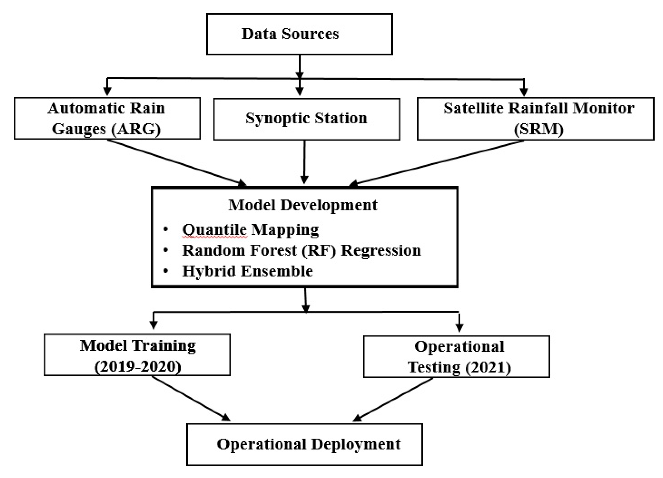
Figure 2.
Study area and location of ARGs and Synoptic Station.
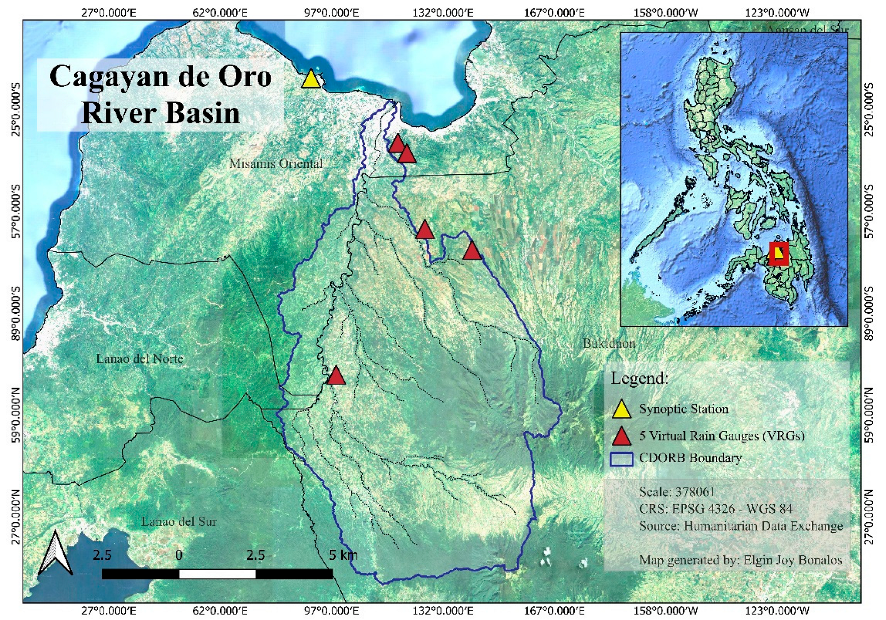
Figure 3.
Temporal comparison of normalized rainfall between averaged (a) ARG network observations and (b) synoptic station.
Figure 3.
Temporal comparison of normalized rainfall between averaged (a) ARG network observations and (b) synoptic station.
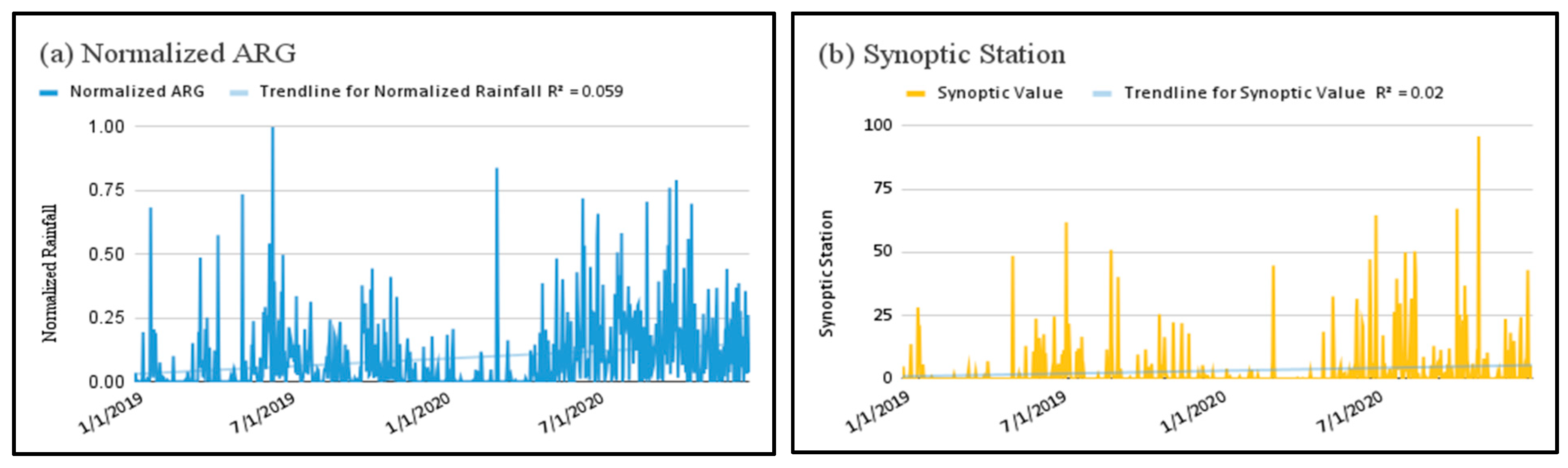
Figure 4.
Scatter plot comparing ARG observations versus uncorrected SRM estimates.
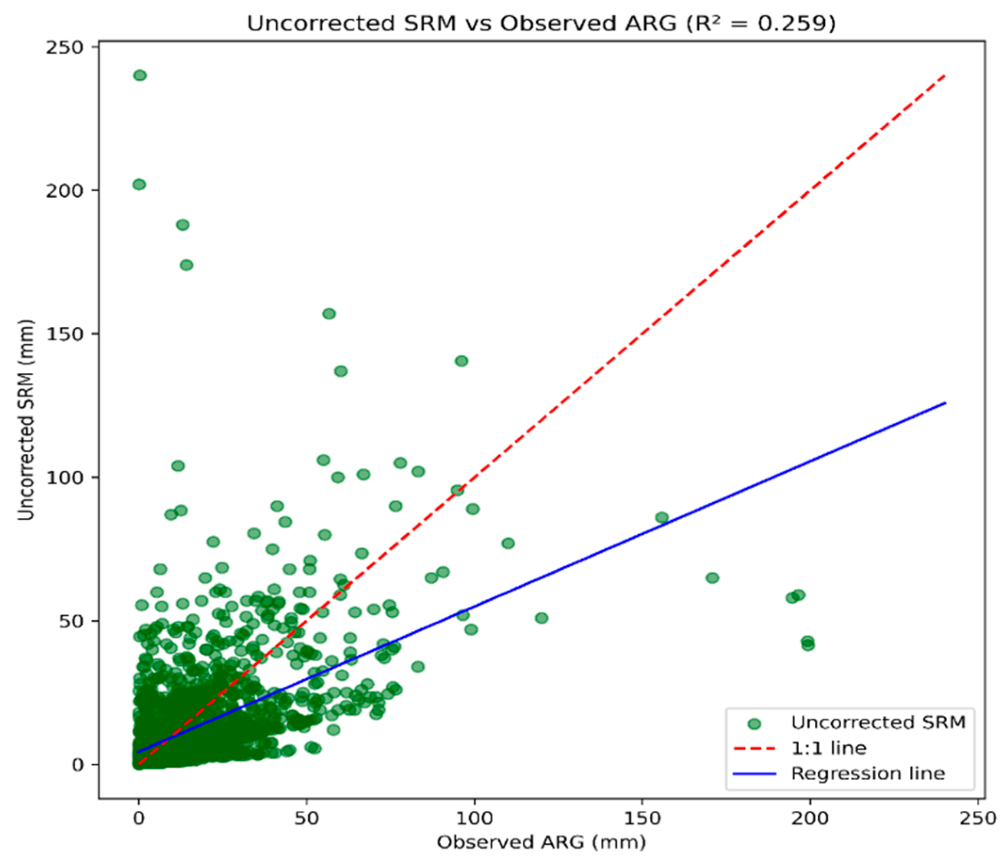
Figure 5.
Scatter plots showing rainfall distribution alignment for Raw SRM, QM, RF, and Hybrid.
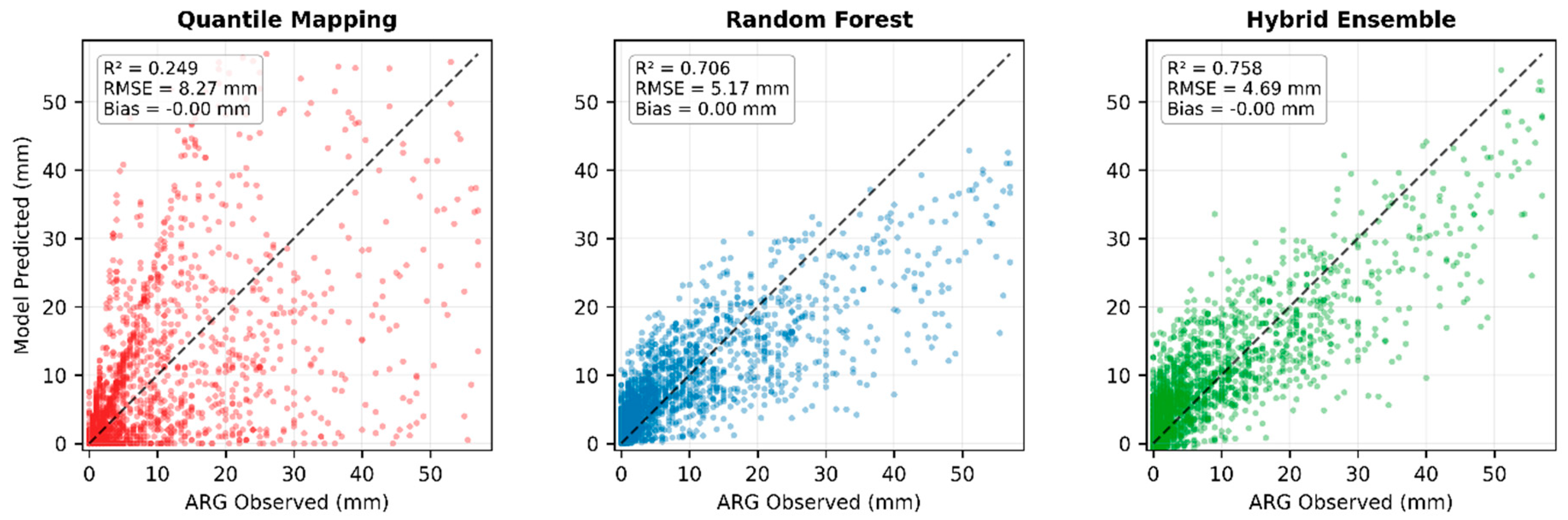
Figure 6.
Empirical CDF of SRM estimates with quartile thresholds and 95% confidence band.
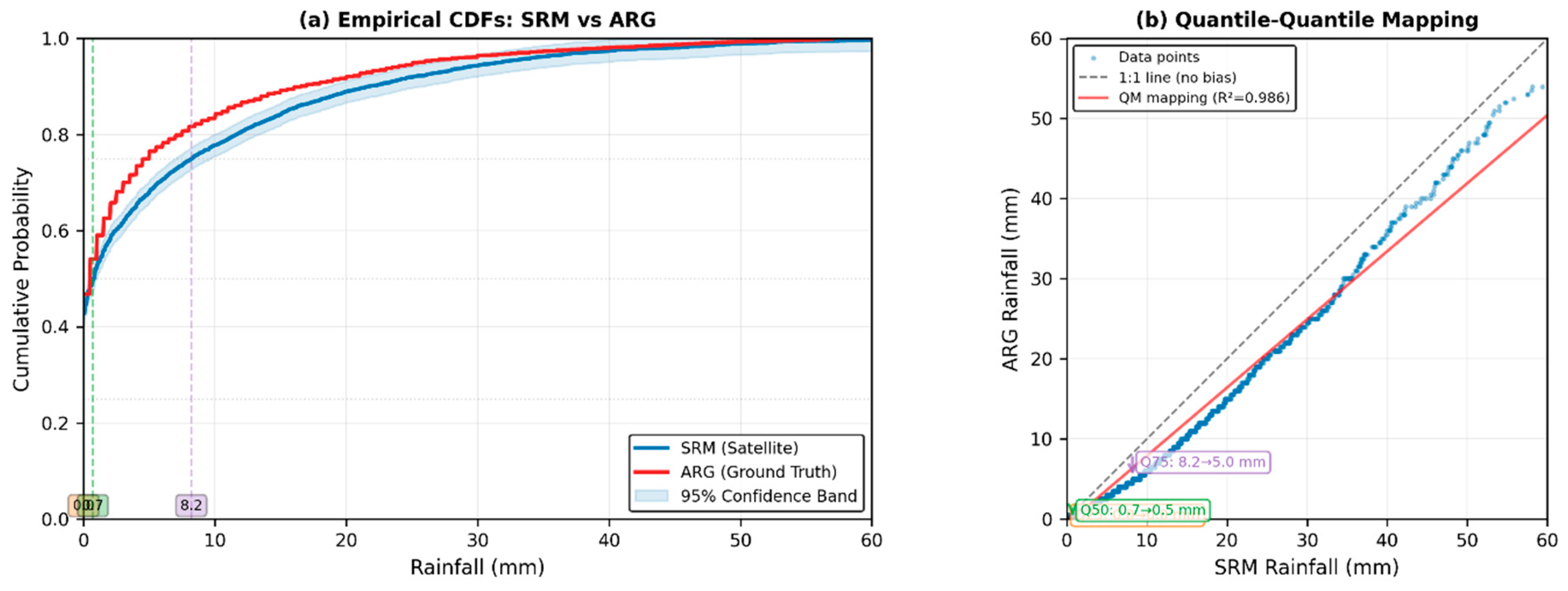
Figure 7.
RMSE comparison across seasons for Raw SRM, QM, RF, and Hybrid models.
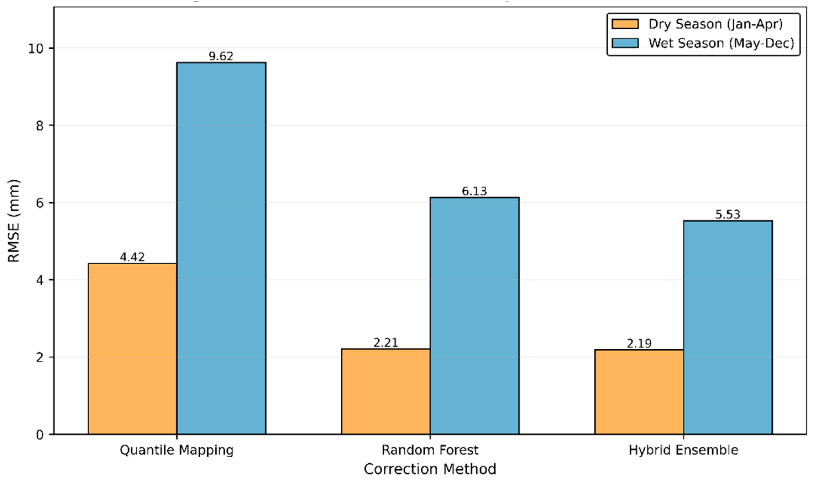
Figure 8.
Scatter plots comparing ARG observations versus model predictions during January–April 2021 testing.
Figure 8.
Scatter plots comparing ARG observations versus model predictions during January–April 2021 testing.
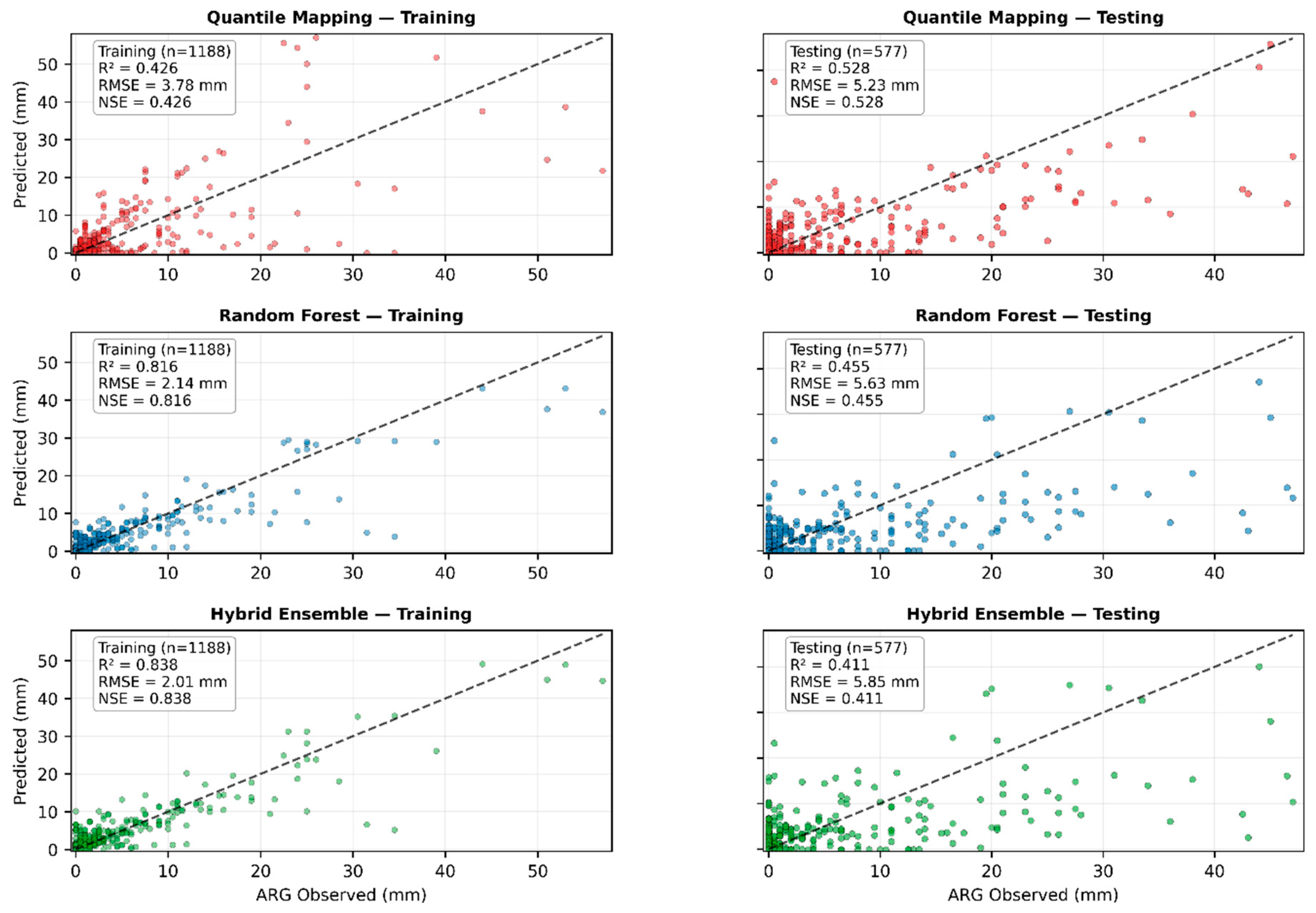
Figure 9.
Performance comparison between training (Jan–Apr 2019–2020) and testing (Jan–Apr 2021) periods, showing R² change (ΔR²) for each correction method.
Figure 9.
Performance comparison between training (Jan–Apr 2019–2020) and testing (Jan–Apr 2021) periods, showing R² change (ΔR²) for each correction method.
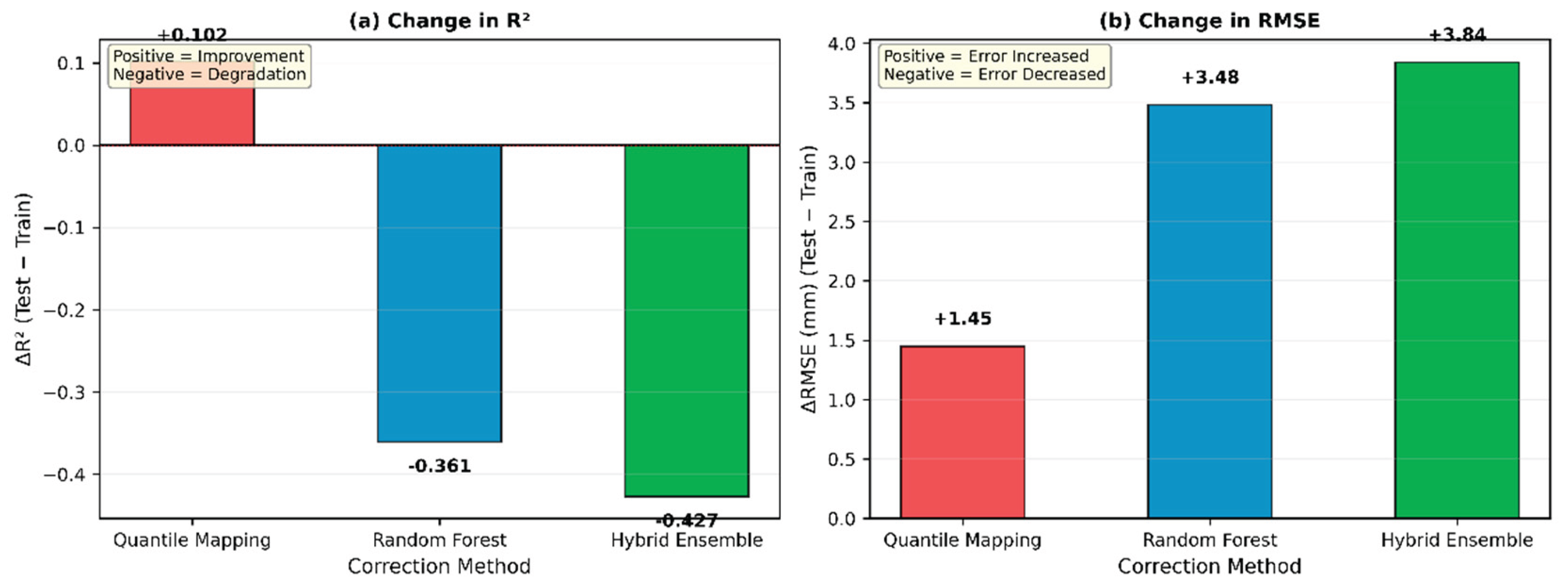
Figure 10.
Operational viability performance of QM, RF, and Hybrid Ensemble.
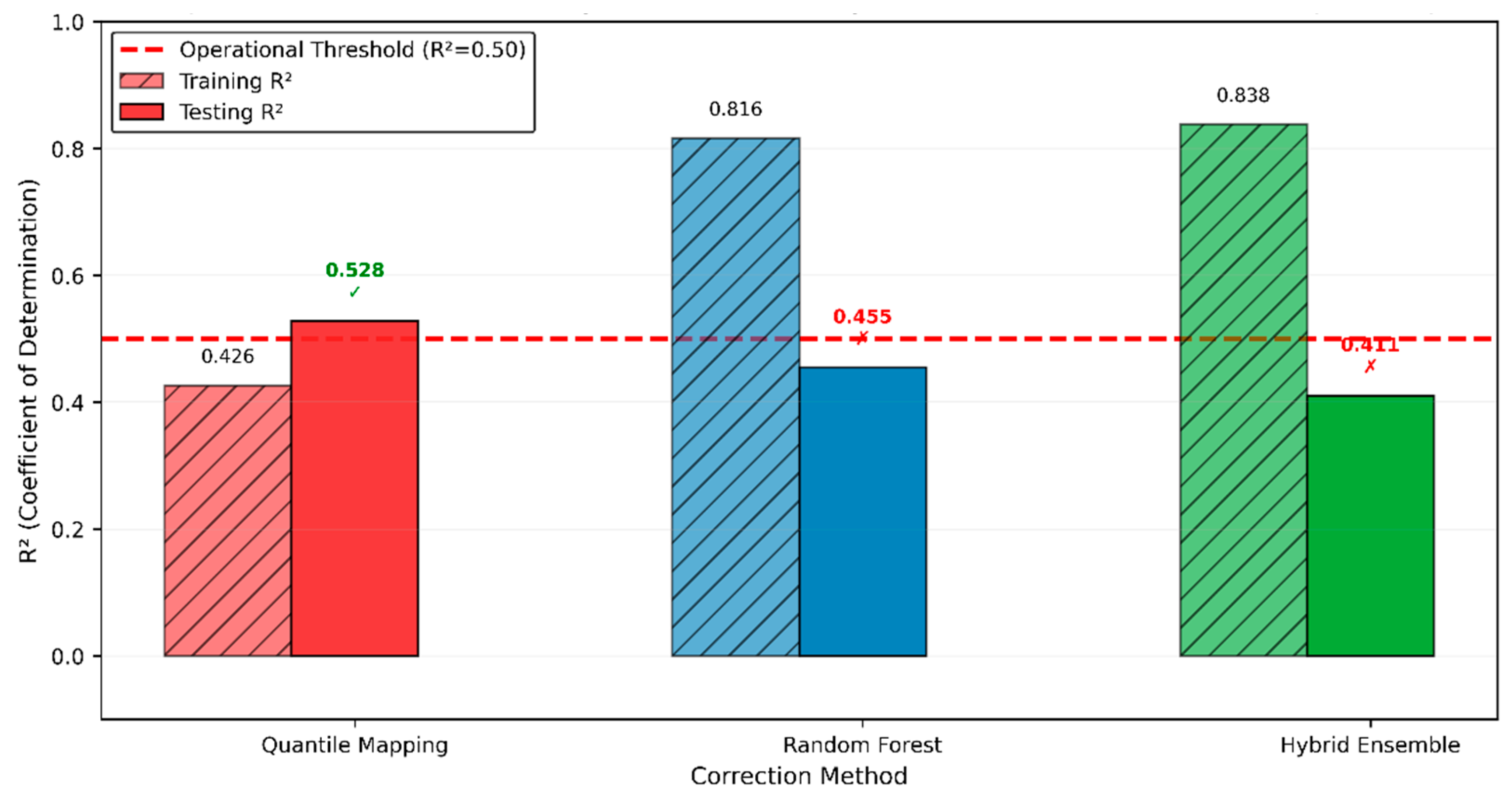
Table 1.
Optimal hyperparameter configuration for the Random Forest Regression (RF) model.
| Parameter | Tested Values | Selected Values |
| N | 100, 200, 300, 400 | 400 |
| depth limits | 5, 10, 20 | 10 |
| minimum samples | 2, 5, 10 | 5 |
Table 2.
Threshold classification for evaluation metrics.
| Metric | Unsatisfactory | Satisfactory | Good | Very Good |
| R2 | < 0.50 | 0.50 - 0.75 | 0.75 - 0.90 | >90 |
| RMSE | > 15 mm/day | 10-15 mm/day | 5 -10 mm/day | <5 mm/day |
| MAE | > 10 mm/day | 6 – 10 mm/day | 3 – 6 mm/day | < 3 mm/day |
| NSE | ≤ 0.50 | 0.50 - 0.65 | 0.65 - 0.75 | 0.75 |
| PBias | > 25 | 15 - 25 | 10 - 15 | < 10 |
Table 3.
Comprehensive Training Performance (2019-2020).
| Model | RMSE (mm) | MAE (mm) | Bias (mm) | NSE | R² |
| QM | 8.27 | 4.90 | -0.005 | 0.25 | 0.25 |
| RF | 5.17 | 2.72 | -0.005 | 0.71 | 0.71 |
| Hybrid Ensemble | 4.69 | 2.85 | ~0 | 0.76 | 0.76 |
Disclaimer/Publisher’s Note: The statements, opinions and data contained in all publications are solely those of the individual author(s) and contributor(s) and not of MDPI and/or the editor(s). MDPI and/or the editor(s) disclaim responsibility for any injury to people or property resulting from any ideas, methods, instructions or products referred to in the content. |
© 2025 by the authors. Licensee MDPI, Basel, Switzerland. This article is an open access article distributed under the terms and conditions of the Creative Commons Attribution (CC BY) license (http://creativecommons.org/licenses/by/4.0/).
Copyright: This open access article is published under a Creative Commons CC BY 4.0 license, which permit the free download, distribution, and reuse, provided that the author and preprint are cited in any reuse.


