
Submitted:
25 December 2025
Posted:
29 December 2025
You are already at the latest version
Abstract
The interrelation between economic growth and financial development have fuelled the debate in the area of economics. The financial development in countries is driven by concert action of the governments in terms of policy making creating favourable financial infrastructures and taking strategic initiatives to building a conducive financial sector. The paper attempts to empirically revisit the association between financial development and long run growth in context of Saudi Arabia. The research uses select variables measured by World bank to predict economic growth and financial development. The research study analyses the link between financial development and economic growth in Saudi Arabia from 1980 to 2020 spanning a 40-year period. It uses a five variable ADRL model using a supply led approach. The Grainger test of causality and the VECM model proposes a unidirectional relationship flowing from proxy of financial development to Economic growth. The paper reports findings that support that financial development leads to economic growth in Saudi Arabia.
Keywords:
Saudia Arabi
; economic growth
; financial development
; ARDL
1. Introduction
The interrelation between economic growth and financial development have fuel support that in the area of economics ever since the contribution of Goldsmith (1969) and McKinnon (1973). Studies have been undertaken by numerous researchers at empirical level and fundamentally researchers have attempted to establish financial development as a precursor to economic development. The financial development in countries is driven by concert action of the governments in terms of policy making creating favourable financial infrastructures and taking strategic initiatives to building a conducive financial sector. The bigger concern in this study has also been how these findings can be interpreted and how the phenomena can be measured as most of the times researchers have been using proxy measures to study the relation between EC and FD.
The paper attempts to empirically revisit the association between financial development and long run growth in context of Saudi Arabia. The research uses select variables measured by IMF and World bank to predict economic growth and financial development. After prolonged state-controlled Saudi Arabian economy which has been fuelled by oil led earnings. The government has been exploring alternative economic avenues to fuel growth. Saudi Arabia economy has seen significant turmoil between 1980-2020 in the early 80’s to mid-80s the economy that was fuelled with oil revenue witnessed a downturn due to recession followed by oil price crashes.
Saudi Arabia reduced its oil production to curb the price fall which affected its oil revenue. In 1990n Saudi Arabia saw stagnating oil prices, decline in real GDP and increase in unemployment. However, the period from 2000 to 2010 was of reforms and recovery economic growth stability was achieved to some extent by increasing the non-oil revenues. Again oil prises saw a collapse in 2015 in response to this the Saudi government launched the vision 2030 programme to boost economic growth it encouraged participation of private sector, building infrastructure projects and improve foreign direct investment in an attempt to reduce dependency on oil revenues. Multiple studies have studied the relationship between (EG) and (FD). Samargandi et. al. 2014 studied the relation between FD and EG with respect to Saudi Arabia. And reported that financial indicator affects non-oil GDP significantly. Ibrahim (2013) study looked at the interrelationship involving EC and EG in the context of SA from 1989 to 2008. The study used OLS (ordinary least square) and found that FD predictors significantly affect EC. Alshammary, (2014) studied the interrelationship between EG and capital market development indicators with respect to SA captured during the period from 1993 to 2009. The ARDL model used in the study reported capital market development indicator to be a significant indicator of EG. The studies on Saudi Arabia have largely been situated in early 2010. The present study covers the period from 1980-2020 a period which is important for SA which is trying to emerging from oil fuelled economy to a nonoil led one. The study also propounds that economic growth in SA had been supply led.
The aim of the research is
- To evaluate the short run and the long-term relationship between economic growth and financial development predictors
- To probe into the direction of causality between the predictor variables in the ARDL model
- To provide strategy policy implicationsfor Saudi government.
2. The Literature on Financial Development and Economic Growth
Economic growth captures production of goods and services in the country and is generally measured by GDP gross domestic production. The increase in production from one period to another is referred to as economic growth the nominal measure for it is generally GNP or GDP. The real measure for economic growth is GDP adjusted for inflation. Another popular measure of economic growth has been the annual GDP growth percentage. Economic growth happens when an economy makes more goods and services. Economic growth can happen when capital goods, labor, technology, and human capital all grow. The total Market Value of new Goods and Services generated is commonly used to measure Economic Growth.
using estimates such as GDP.
Numerous indication showing that economic growth is driven by financial development. (Kamal 2003 )studied the impact of mobilising saving, ensuring control, assigning funds and increasing innovation is a key to economic growth.The theoretical link between Financial development and Economic was further confirm by Schumpeter (1911) whose work explores the relationship between EG and FD and stress the need for financial services in countries.
However, researchers have been questioning the relationship between FD and EG as an economic system grows need for financial services also grows thus questioning the FD to EG nexus (Robinson 1960). The bi-directional nature of the relationship can be summarised into two well developed competing concepts. The first being demand- push which supports the thought process that financial development happens due to the push from economic growth. As against this the supply led approach proposes that FD to EG happens as countries develop robust financial institutions which promote financial services required for EG. It is to be understood the economic growth is an intricate process affected by multitude of factors, thus isolating the causal role of financial development in its creation is often difficult.
Financial Development
The financial development in most economies has been powered by strategic actions like the reforms in the banking system, liberalisation of the government policy and development in the capital markets.
Encouraging growth and expansion of banking system was considered a significant precursor to economic growth(Gurly & Shaw, 1960; Goldsmith, 1969). Demetriades & Luintel in 1996 proposed that the banking system controlled the interest rate which impacted the relationship between financial development and economic growth in Indian economy. Different from previous study which used aggregated macroeconomic data Neusser and Kugler (1998) sought to comprehend the correlation between industrial sector GDP, financial sector GST, and overall productivity.
The supply- push which support the fact that it is the economic development in a country can be energised by a financial development (Patrick 1966). He was the first economist who studied the causal relation and directional relation empirically. He suggested that measures like interest softening better access to financial services and better information flow stimulates the economy for a more productive environment.
The neo-liberal school promotes market led reforms and financial liberalisation, whose most important theorists are (McKinnon, 1973) and (Shaw, 1973). (Roobini & Martin 1995) explored the position of government policy and financial development their model states that government policies can both be restrictive or enabler in the financial markets. It has been observed that tendency of tax evasion often leads to restrictive policies by government in turn generating high inflation tax. Since restricted policies lower productivity of capital and hampers growth. With a different view De Gregorio (1993) studied saving rates and how they get affected by financial market developments. They concentrated on borrowing restrictions and economic growth. Their study showed that relaxing borrowing constraint often leads to increase in economic growth. Positive relationship between growth in real interest rate was observed by Dornbusch 1988 irrespective of the channel of transmission. However, he reported that savings are not related to the level of real interest rates. Fry (1989) in contrast to the above finding reported a strong positive effect of real interest rates on financial savings. The efficiency of capital accumulation can be well represented by positive real interest rates as suggested by Khan and Villanueva 1991.Calvo & Coricelli (1992) reported that real interest rate often reflect fragile financial structure and reduced regulatory setting the study was based in Eastern European economies.
(Romer, 1986: Lucas, 2009), presented the Dynamic endogenous growth model which provided support to the relationship between EG and FD (King & Levine 1993).The assumption of the endogenous model is that fiscal intermediaries offer the country with numerous classes of benefits like lowering investment, liquidity and productivity risks, facilitating information for better decision making. The service provided by intermediaries help in improving effectiveness and level of investment. This in turn leads to economic growth as per the endogenous model. Study based on capital allocation in investment and its impact on financial structure was developed by Greenwood & Jovanovic (1990) who suggested that based on capital accumulation there is a positive influence of financial structure on growth. Ben Habib & Spiegel in 2000 proposed the model where financial development provided positive relationship with total productivity. Beck et al. ( 2000) reported positive association linking FD and total factor output which overall impacts GDP growth which also found support in other studies (Kunt & Levine, 2008; King & Levine, 1993; Demetriades & Hussein, 1996; Khan & Senhadji, 2000).
The Nexus between FD and EG has addressed controversial issues of causality. The earlier studies explored the relationship based on various foundations proposed by economist. Empirical results show that the direction of causality is sensitive to the indicator used for FD while some indicators confirm the relation the others may show contradictory result. The causal association linking FD and EG has been studied both in long term and short-term using regression study. Although the present results are suggestive of a positive relationship which depends upon the predictor used as the alternate for FD. The context of the study in terms of countries economics, endogeneity and heterogeneity are issues also being looked at in the new studies.
Financial Development Measures
Another important concern along with the direction of relationship between EG and FD has been around the indicators of FD. Most researchers have known do you use macro economical, banking or fiscal indicators as proxy measures for FD. The literature use diverse indicators to represent the “level of financial development,” including interest rates, monetary aggregates, and the ratio of the banking system’s size to GDP (Al-Awad & Harb, 2005; Chuah & Thai, 2004; among others).
A critical point in understanding the relationship between FD and EG is finding a valid indicator for FD. Frequently used indicator of FD is derived by the measure of money narrow money and broad money as a share to nominal revenue (King & Levine, 1993; Wood, 1993; Murinde & Eng, 1994; Lyons & Murinde, 1994; Berthelemy & Varoudakis, 1995; Arestis & Demetriades, 1997; and Agung & Ford, 1998).M2 and M3 are suggested for use as a less liquid monetary aggregate (Gregorio & Guidotti ,1995). Another popular proxy for FD is BDY (Bank deposit liabilities to income) it known to be higher in developed economies as it reflects the rigorous use of money rather than increasing deposits. (Demetriades & Hussein, 1996; Luintel & Khan, 1999).
Domestic credit to income DCY positively linked to price signalling in terms of real interest rates can be used as a proxy forFD (Odedokun, 1989). Similarly private sector credit (CPY) proportion may be used, The loan given to the business community can encourage investments and output, which can then contribute to economic growth.
The IMF has developed several indexes that can be used to measure financial development in an economy (Svirydzenka, 2016).
3. Methodology
The study duration was from 1980 to 2020 which includes a period of liberalisation, reforms and development in Saudi Arabia. During this period SA also saw an increase in monetary growth and improvement in investments in the non-oil sector. The data spans 40 years and is enough for an ARDL model to study the interrelationship between EG and FD. The study also revisited the debate on causality between EG and FD.
Dependent Variable
GDP per capita growth rate was considered as an alternate to study economic growth.
Independent Variable
The study explores five independent variables to be used as surrogates for financial development. We drew these indicators from banking sector financial intermediaries and monetary & fiscal policy measures.
Domestic loans provided by banks as a percentage of GDP(DCBS) was the first important indicator. Higher DCBS indicates dependency of corporate sector on banks for funding. It is an indicator of financial development in the country. Banks are more likely to drive investment in a country.
Domestic credit to private sector can be considered as the second indicator for FD it is measured using credit to the private sector as a percentage of GDP it measures the level of its mention that flows to private sector higher level of DCPS means the economy is diversity from government to private sector.
The third proxy is broad money as a percentage of GDP it measures the liabilities of the banking sector India country empty is often referred to as the measure of financial debt of the sector. Invent M2 are not considered good indicators as they ability to channelize loans from saving to borrow is limited (Khan & Senhadji, 2000).
Gross domestic saving (GDS) as a percentage of growth rate what is the fourth financial development indicator. (Pagan 1999) reports that (GDS) affects EG ensuring that a significant percentage of the saving is devoted to investments. Subscript
The fifth measure of FD is FCE (final consumption expenditure). It measures the size of the financial sector and the significance of fiscal policy. It shows which sectors are being encouraged to grow by ensuring flow of investment by government. FCE is measured as percentage of government expenditure to GDP growth.
To study the order of integration of all the variables the ADF (Augmented Dickey Fuller test) was conducted. All variables were first tested for stationarity at first level and subsequently where also tested for first differences. The Table 1 shows that all the variables are integrated at different levels.
GDPPC, M3 , GDS and FCE are integrated at first difference. DCBS is not integrated at either first level or first difference and DCPS is integrated at first level.
Empirical Results
Given by the endogenous growth literature (Rosen1986; King & Levine 1993 )the role of financial development and economic growth is established it is expected that mobilization of the financial sector through financial services investment and allocation of resources facilitates economic growth Roubini & i-Martin. (1995)
Cointegration test
Interpretation of cointegration
Null hypothesis =No Cointegration between independent variables
Alternate Hypothesis = Cointegration exist between independent variables
To analyse the cointegration properties of the estimated equation the ARDL integration process was used. One of the advantages of testing method is that it can be applied whether regressors in the equation of stationary or nonstationary to analyse
Table 2 provides the computed value of the F-statistics for testing the existence of a long run change GDPCC equation under the null hypothesis i.e., No Cointegration between independent variables. The F statistics is compared with I(0) value if it is less than it we accept the null hypothesis. However, the value more that the critical value at I(1) we reject the null hypothesis. In the present case at one percent critical value I(0)is 5.018 and I(1) it is 6.61 since the test value is 8.13 which is more than 6.61, we will reject the null hypothesis and accept the alternate hypothesis and say that M3/GDP, FCE/GDP and GDS/GDP are cointegrated at one percent level.
Compare the test value with the critical value at 5 percent level of significance. If the test Statistics is greater than critical value, we reject the null hypothesis. We start with r=0 at this level we rejected the null hypothesis. We moved to r=1at this level we failed to reject the null hypothesis thus accepting the alternate hypothesis that two vectors are cointegrated.
Econometric Model
The Autoregressive Distributed Lags (ARDL) model is employed to examine the determinants influencing the economic growth measured by GDPPC. Shin and Pesaran (1999) and Pesaran et al. (2001) made this model, which is explained by the following equation:
It shows that the dependent variable yt is based on the vector of dynamic explanatory variables and their lagged values xt. Lastly, εt is an error term that is the same as a mean value of zero. This model is defined by its capacity to accommodate a mixture of integrated variables of varying degrees I (0) and I (1), suitable for our case.
The present study used five proxy for financial development of the five only three variables were having significant relationship with economic growth as shown in Table 4.
Econometric Model
The Autoregressive Distributed Lags (ARDL) model is employed to examine the determinants influencing the economic growth measured by GDPPC. Shin and Pesaran (1999) and Pesaran et al. (2001) made this model, which is explained by the following equation:
It shows that the dependent variable yt is based on the vector of dynamic explanatory variables and their lagged values xt. Lastly, εt is an error term that is the same as a mean value of zero. This model is defined by its capacity to accommodate a mixture of integrated variables of varying degrees I (0) and I (1), suitable for our case.
The present study used five proxy for financial development of the five only three variable were having significant relationship with economic growth as shown in table:
Where
=GDP per capita growth rates
- These can include a wide range of items such as cash, stocks, bonds, real estate, inventory, equipment, patents, and investments, and are held by individuals, households, and companies within that country
- is the ratio of gross domestic savings to GDP
- government final consumption expenditure to GDP

Table 3.
Johansen-Procedure: Test statistic.
| test | 10pct | 5pct | 1pct | |
| r ≤ 3 | 0.13 | 6.5 | 8.18 | 11.65 |
| r ≤ 2 | 12.81 | 15.66 | 17.95 | 23.52 |
| r ≤ 1 | 39.01 | 28.71 | 31.52 | 37.22 |
| r = 0 | 81.33 | 45.23 | 48.28 | 55.43 |
Table 4.
The long-term relation between economic growth and financial development.
| Estimate | Std. Error | t value | Pr(>|t|) | |
| (Intercept) | -15.91620 | 4.41209 | -3.607 | 0.00148 ** |
| GDS.t | 0.27083 | 0.10606 | 2.554 | 0.01775 * |
| GDS t-1 | 0.37680 | 0.17370 | 2.169 | 0.04065 * |
| GDSt-2 | 0.15947 | 0.12747 | 1.251 | 0.22350 |
| M3.t | 0.05109 | 0.17091 | 0.299 | 0.76766 |
| M3.t-1 | -0.12021 | 0.22052 | -0.545 | 0.59092 |
| M3.t-2 | 0.48906 | 0.17438 | 2.805 | 0.01006 * |
| FCEt | -0.25719 | 0.28804 | -0.893 | 0.38116 |
| FCEt-1 | 1.00728 | 0.34897 | 2.886 | 0.00833 ** |
| FCEt-2 | -0.94240 | 0.28096 | -3.354 | 0.00275 ** |
| GDPPC.1 | 0.05963 | 0.16432 | 0.363 | 0.72002 |
| GDPPC.2 | -0.05195 | 0.11838 | -0.439 | 0.66488 |
| GDPPC.3 | 0.05202 | 0.11075 | 0.470 | 0.64303 |
| GDPPC.4 | -0.05789 | 0.10519 | -0.550 | 0.58738 |
| Adjusted R-squared | 0.627 | |||
| F | 5.667 | 0.000158 |
The super script shows the significance level =*** at 0.001,** at 0.01 and * at 0.05.
The ARDL model shows that domestic credit to the private sector and domestic credit as a percentage of GDP are not significant predictors of GDPPC and henceforth dropped from the final Model. Table 4 shows the results of the econometric model and the long-term relationship between predictors of economic growth. Gross domestic saving had a positive impact on GDP growth both at the current level as well as at the first lagged value.M3 has a positive impact on GDPPC at lagged value t-2. Government Expenditure had mixed findings at lag value t1; it had a negative impact on GDPPC, while at lagged value t2, it had a positive impact on GDPPC. The model was robust, and the predictor variables explained 62.7 percent of the variation in GDPPC as seen by the R-squared value in Table 4.
Error Correction Model
To conduct a comprehensive investigation of the drivers of GDPPC in SA, it is essential to estimate an ARDL error-correction model to identify short-run correlations among variables. The results are shown in Table 5 as follows:
Table 5.
The ECM -the short-term relationship between economic growth and financial development.
| Estimate | Std. Error | t value | Significance | |
|---|---|---|---|---|
| (Intercept) | -11.98761 | 2.47219 | -4.849 | 6.79e-05*** |
| ec.1 | -0.68049 | 0.19035 | -3.5749 | 1.31e-05*** |
| GDSt | 0.24437 | 0.09503 | 2.572 | 0.017058* |
| GDSt-1 | -0.2593 | 0.11031 | -2.351 | 0.027691* |
| M3.t | -0.04214 | 0.1367 | -0.308 | 0.760667 |
| M3t-1 | -0.47084 | 0.15327 | -3.072 | 0.005394** |
| FCE.t | -0.44088 | 0.21424 | -2.058 | 0.051107 |
| FCEt-1 | 0.82566 | 0.20412 | 4.045 | 0.000503*** |
| FCEt-2 | -0.49837 | 0.22938 | -2.173 | 0.040354* |
| dGDPPC.1 | 0.18461 | 0.14832 | 1.245 | 0.225788 |
| dGDPPC.2 | -0.03738 | 0.13416 | -0.279 | 0.782999 |
| dGDPPC.3 | 0.10225 | 0.11055 | 0.925 | 0.364578 |
| dGDPPC.4 | 0.07071 | 0.09557 | 0.74 | 0.466864 |
| Adjusted R-squared | 0.756 | |||
| F | 9.968 | 0.00018 |
The super script shows the significance level =*** at 0.001,** at 0.01 and * at 0.05.
The error correction term reflects the impact of deviations from the long-run equilibrium. The error correction term in each equation indicates how each variable tends to restore equilibrium in the change in GDPPC. The results in Table 5 shown above indicate that the error correction term is negative and significant, and its value is (-0.68), which means that a return to equilibrium in the dynamic model is possible, and therefore the variation that occurs in the short term is corrected annually (given that the data are annual). The negative coefficient indicates that the deviation from the long-term equilibrium is corrected at a rate of almost 68 percent.
Granger’s Causality Test
The test for cointegrating indicates that at least two vectors are cointegrated as they share a common trend. Since the relevant variables have a common trend, Granger causality must exist at least in one direction (Granger, 1988).
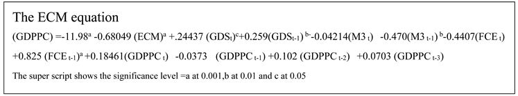
Table 6: Granger’s causality
Applying the Granger’s causality approach demonstrates that a unidirectional causality is running from M3 to GDPPC and from FEC to GDPPC. This further strengthens the supply-led growth model of economic development being used in this study.
Table 7.
Diagnostic tests to gauge the adequacy of the specifications of the model.
| p-value = | |||
|---|---|---|---|
| Ramsey’s RESET Test for model specification | 1.9307 | df1 = 2, df2 =22 | 0.1786 |
| Shapiro-Wilk test of normality of residuals | 0.97861 | 0.6982 |
|
| Breusch-Pagan Test for the homoskedasticity of residuals | 9.5626 | df = 13 | 0.8463 |
| Ljung-Box Test for the autocorrelation in residuals | 3.2749e-06 | df = 1 |
0.9986 |
| Breusch-Godfrey Test for the autocorrelation in residuals |
4.6068e-06 | df1 = 1, df2 =19 | 0.9983 |
Traditional tests are used to diagnose the model according to its assumptions. Independence of error equations 2 and 3 is required to test for serial correlation. The Breusch-Godfrey Test is used for autocorrelation in residuals. The Shapiro-Wilk test assesses the normality of residuals. The Breusch-Pagan Test evaluates homoskedasticity of residuals.
The CUSUM and CUSUM squared test proposed by Brown et al. (1975) can be applied to test the stability of the long-term relation between GDPPC and its predictor. The test is applied to the residuals of the model. If the plots remain within the boundary at 5% significance, then stability is confirmed. If we see Figure 1, we see that the line stays within the boundary indicated by the red line in both graphs, validating the stability of the GDPPC equation.
4. Discussion and Conclusion
The empirical finding studied co-integration, Granger’s causality, and the short and long-term underlying forces in the causal relation between EC and FD. We have applied the ARDL Bounds Testing approach to determine the cointegration, the Error Correction Model (ECM) for long and short-run dynamics, and the Granger Causality test in the VECM framework. The empirical finding reported that the following variables were predictors of GDPPC.
GDS is important for every country as it saves favour economic growth by encouraging investment and capital formation (Kazmi 1993). Mboweni (2008) proposes that GDS safeguards economies from bankruptcy, devaluation of currency, and inflation. GDS has a positive and significant impact on GDPPC growth. The GDS has a mixed impact on GDPPC; it all depends on where the savings are channelized. It has both a current as well as a lagged impact.
M3 is commonly referred to as broad money and has been used as a Financial development by Darat 1999 and Kar et al. 2011. It is a General measure of monetisation variable as used by
King &Levine1993 and measure the size of the financial market and its depth. An increase in M3 indicates the expansion in financial intermediaries. The findings of the present study reiterate the impact of M3; however, the impact is lagged t-2, indicating a delayed impact.
On one hand government can fuel economic growth by allocating resources to sectors that can drive economic growth. On the other hand, the government can’t spend a lot of money since it needs to borrow money and pay taxes to do so. But borrowing might make investments more expensive, push private investments out of the way, and raise taxes in the future. Therefore, one says that government expenditure has both positive and negative impacts on economic growth. The same is also demonstrated in the findings of the study, the lagged effect is positive while the current effect is negative.
Taking all this into consideration, the Saudi Arabian government should review its existing policy interventions to promote economic growth. The present study provides a road map to the government and a clear direction for financial interventions that may help it to grow the economy in a particular direction. The final consumption expenditure of the government should be channelised to investment that increases GDPPC enhancing sectors, and help the economy to grow. From a policy standpoint, any solitary or individual policy initiative on macroeconomic variables such as GDS, FCE, and M3 would not yield good outcomes. So, a policy that combines different macroeconomic variables will help a country like SA.
Funding Statement: This work was supported and funded by the Deanship of Scientific Research at Imam Mohammad Ibn Saud Islamic University (IMSIU) (grant number IMSIU-DDRSP2504).
References
- Agung, F.; Ford, J. Financial Development, Liberalization And Economic Development in Indonesia, 1966-1996: Cointegration and Causality. University Of Birmingham, Department Of Economics Discussion Paper 1998, No, 98–12. [Google Scholar]
- Al-Awad, M.; Harb, N. Financial development and economic growth in the Middle East. Applied Financial Economics 2005, 15(15), 1041–1051. [Google Scholar] [CrossRef]
- Alshammary, M. Financial development and economic growth in developing countries: Evidence from Saudi Arabia. Corporate Ownership and Control 2014, 11(2), 718–742. [Google Scholar] [CrossRef]
- Arestis, P.; Demetriades, P. “Financial Development and Economic Growth: Assessing the Evidence”. Economic Journal 1997, 107(442), 783–799. [Google Scholar]
- Beck, T; Levine, R; Loyaza, N. Finance and the sources of growth. Journal of Finance and economics 2000, 58, 261–300. [Google Scholar] [CrossRef]
- Benhabib, J; Spiegel, MM. The role of financial development in growth and investment. Journal of Economic. Growth 2000, 5, 341–360. [Google Scholar] [CrossRef]
- Berthelemy, J.C.; Varoudakis, A. “Thresholds In Financial Development And Economic Growth”. Manchester School Of Economic And Social Studies 1995, 63, 70–84. [Google Scholar] [CrossRef]
- Brown, R. L.; Durbin, J.; Evans, J. M. Techniques for testing the constancy of regression relationships over time. Journal of the Royal Statistical Society Series B: Statistical Methodology 1975, 37(2), 149–163. [Google Scholar] [CrossRef]
- Calvo, G. A.; Coricelli, F. Stabilizing a previously centrally planned economy: Poland 1990. Economic Policy 1992, 7(14), 175–226. [Google Scholar] [CrossRef]
- Chuah, H. L.; Thai, W.; Chuah, L. Financial development and economic growth: Evidence from causality tests for the GCC countries. In IMF Working Papper; 2004. [Google Scholar]
- Darrat, A. F. Are financial deepening and economic growth causally related? Another look at the evidence. International Economic Journal 1999, 13(3), 19–35. [Google Scholar] [CrossRef]
- De Gregorio, J. Inflation, taxation, and long-run growth. Journal of monetary economics 1993, 31(3), 271–298. [Google Scholar] [CrossRef]
- De Gregorio, J.; Guidotti, P. E. Financial development and economic growth. World development 1995, 23(3), 433–448. [Google Scholar] [CrossRef]
- Demetriades, P. O.; Hussein, K. H. Does financial development cause economic growth? Timeseries evidence from 16 countries. Journal of Development Economics 1996, 51, 387–411. [Google Scholar] [CrossRef]
- Demetriades, P. O.; Luintel, K. B. Financial development, economic growth and banking sector controls: evidence from India. The Economic Journal 1996, 106(435), 359–374. [Google Scholar] [CrossRef]
- Demirguc-Kunt, A.; Demirguc-Kunt, A.; Levine, R. Finance and economic opportunity; World Bank: Washington, DC, 2008. [Google Scholar]
- Dornbusch, R. Exchange Rates and Inflation; MIT Press, 1988. [Google Scholar]
- Fry, M. J. Savings, investment, growth and financial distortions in Pacific Asia and other developing areas. international economic journal 1998, 12(1), 1–24. [Google Scholar]
- Goldsmith, R. W. Financial structure and development; Yale: New Haven, CT, 1969. [Google Scholar]
- Granger, C. W. Some recent development in a concept of causality. Journal of econometrics 1988, 39(1-2), 199–211. [Google Scholar] [CrossRef]
- Greenwood, J.; Jovanovic, B. Financial development, growth, and the distribution of income. Journal of political Economy 1990, 98(5(Part 1), 1076–1107. [Google Scholar] [CrossRef]
- Gurley, J. G.; Shaw, E. S. Financial structure and economic development. Economic development and cultural change 1967, 15(3), 257–268. [Google Scholar] [CrossRef]
- Ibrahim, M. A. Financial development and economic growth in Saudi Arabian economy. Applied Econometrics and International Development 2013, 13(1), 133–144. [Google Scholar]
- Kamal, M. Financial development and economic growth in Egypt: A re-investigation. Available at SSRN 2297228; 2013.
- Kar, M.; Nazlıoğlu, Ş.; Ağır, H. Financial development and economic growth nexus in the MENA countries: Bootstrap panel granger causality analysis. Economic modelling 2011, 28(1-2), 685–693. [Google Scholar] [CrossRef]
- Kazmi, A. A. A Study on Saving Functions for Pakistan: The Use and Limitations of Econometric Methods. The Lahore Journal of Economics 2001, 6(2), 57–101. [Google Scholar] [CrossRef]
- Khan, M. S.; Villanueva, D. Macroeconomic policies and long-term growth: a conceptual and empirical review. African Economic Research Consortium special paper; 1991; 13. [Google Scholar]
- Khan, S.M.; Senhadji, A.S. Financial development and economic growth:an overview. IMF Working Paper 00/209, Washington, DC; 2000. [Google Scholar]
- Lucas, R. E., Jr. Ideas and growth. Economica 2009, 76(301), 1–19. [Google Scholar] [CrossRef]
- Luintel, K. B.; Khan, M. A quantitative reassessment of the finance–growth nexus: evidence from a multivariate VAR. Journal of development economics 1999, 60(2), 381–405. [Google Scholar] [CrossRef]
- Lyons, S.E.; Murinde, V. “Cointegration And Granger-Causality Testing Of Hypotheses On Supply-Leading And Demand-Following Finance”. Economic Notes 1994, 23(2), 308–316. [Google Scholar]
- McKinnon, R. I. The value-added tax and the liberalization of foreign trade in developing economies: a comment. Journal of Economic Literature 1973, 11(2), 520–524. [Google Scholar]
- Murinde, V.; Eng, F.S.H. “Financial Development and Economic Growth In Singapore: Demand-Following Or Supply-Leading?”. Applied Financial Economics 1994, 4(6), 391–404. [Google Scholar] [CrossRef]
- Neusser, K.; Kugler, M. Manufacturing growth and financial development: evidence from OECD countries. Review of economics and statistics 1998, 80(4), 638–646. [Google Scholar] [CrossRef]
- Odedokun, M.O. “Causalities Between Financial Aggregates and Economic Activities in Nigeria: The Results from Granger’s Test”. Savings and Development 1989, 23(1), 101–111. [Google Scholar]
- Pagano, M. Financial markets and growth: an overview. European Economic Review 1993, 37, 613–622. [Google Scholar] [CrossRef]
- Patrick, H. T. Financial development and economic growth in underdeveloped; 1966. [Google Scholar]
- Pesaran, M. H.; Shin, Y.; Smith, R. J. Bounds testing approaches to the analysis of level relationships. Journal of applied econometrics 2001, 16(3), 289–326. [Google Scholar] [CrossRef]
- Robinson, E. A. G. Economic Consequences of the Size of Nations; Palgrave Macmillan, 1960. [Google Scholar]
- Romer, P. M. The origins of endogenous growth. Journal of Economic perspectives 1994, 8(1), 3–22. [Google Scholar] [CrossRef]
- Rosen, S. The theory of equalizing differences. Handbook of labor economics 1986, 1, 641–692. [Google Scholar]
- Roubini, N.; Sala-i Martin, X. “Financial Repression and Economic Growth”. Journal of Development Economics 1992, 39, 5–30. [Google Scholar] [CrossRef]
- Roubini, N.; Sala-i-Martin, X. A growth model of inflation, tax evasion, and financial repression. Journal of Monetary Economics 1995, 35(2), 275–301. [Google Scholar] [CrossRef]
- Samargandi, N.; Fidrmuc, J.; Ghosh, S. Financial development and economic growth in an oil-rich economy: The case of Saudi Arabia. Economic modelling 2014, 43, 267–278. [Google Scholar] [CrossRef]
- Schumpeter, Joseph. The Theory of Economic Development; Harvard University Press: Cambridge, Mass., 1911] 1934. [Google Scholar]
- Shaw, E. S. Financial deepening in economic development; Oxford University Press: New York, 1973. [Google Scholar]
- Svirydzenka, K. Introducing a new broad-based index of financial development; International Monetary Fund, 2016. [Google Scholar]
- Wood, A. “Financial Development and Economic Growth In Barbados: Causal Evidence”. Savings And Development 1993, 17(4), 379–390. [Google Scholar]
Figure 1.
.
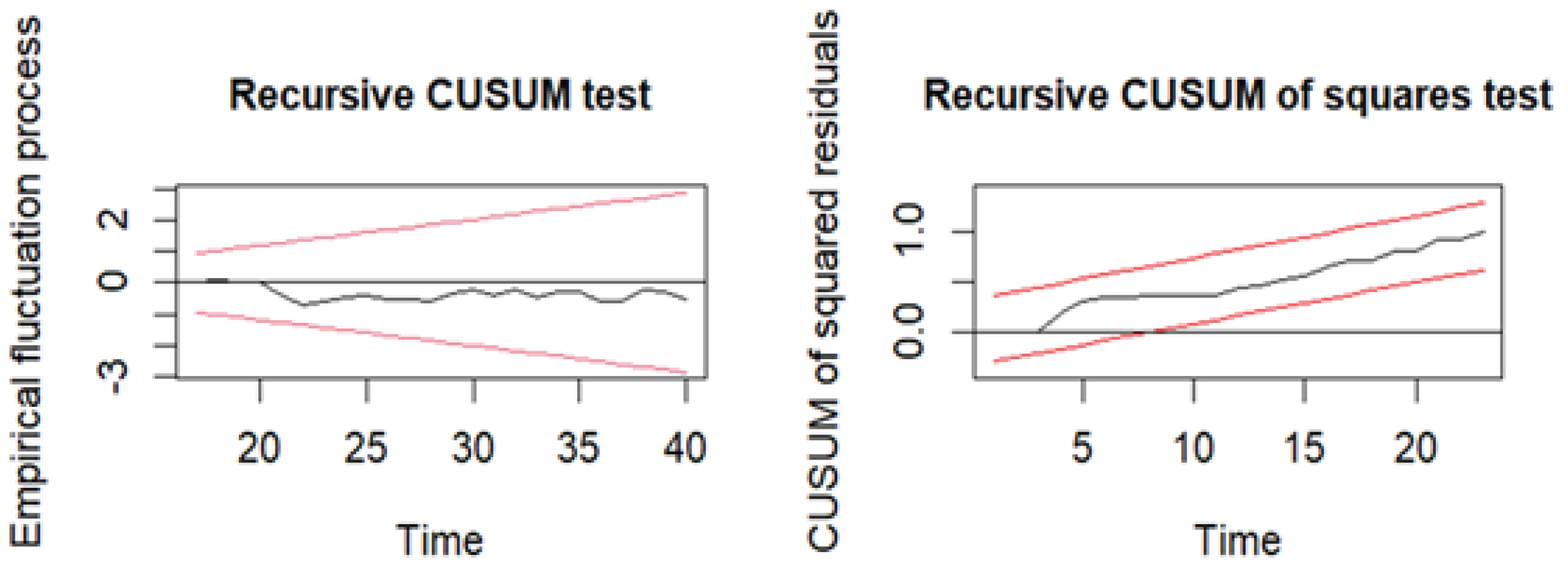
Table 1.
ADF Unit root tests.
| I(0) | I(I) | |||
|---|---|---|---|---|
| Dickey-Fuller | p-value | Dickey-Fuller | p-value | |
| GDPPC | -2.6806 | 0.3 | -3.928 | 0.02 |
| M3 | -3.0425 | 0.16 | -3.8376 | 0.02 |
| GDS | -1.6763 | 0.7 | -3.5241 | 0.05 |
| FCE | -1.4555 | 0.78 | -3.5375 | 0.05 |
| DCBS | -1.2340 | 0.56 | -2.6031 | 0.16 |
| DCPC | -1.2108 | 0.88 | -4.5703 | 0.01 |
Table 2.
Cointegration Test (Pesaran, Shin and Smith,2001).
| Significance Level | 1(0) | 1(1) | |
|---|---|---|---|
| 10% | 2.933 | 4.02 | |
| 5% | 3.548 | 4.803 | |
| 1% | 5.018 | 6.61 | |
| F-statistic | 8.14 |
Table 6.
Granger’s causality.
| Independent variable | ||||
|---|---|---|---|---|
| Dependent variable | GDPCC | M3 | GDS | FCE |
| GDPCC | 0.0033 | 0.068 | 1.4007 | |
| M3 | 11.057*** | 5.9418 ** | 0.5354 | |
| GDS | 2.54* | 0.4951 | 15.6*** | |
| FCE | 0.3966 | 9.1868*** | 0.352 | |
The super script shows the significance level =*** at 0.001,** at 0.01 and * at 0.05.
Disclaimer/Publisher’s Note: The statements, opinions and data contained in all publications are solely those of the individual author(s) and contributor(s) and not of MDPI and/or the editor(s). MDPI and/or the editor(s) disclaim responsibility for any injury to people or property resulting from any ideas, methods, instructions or products referred to in the content. |
© 2025 by the authors. Licensee MDPI, Basel, Switzerland. This article is an open access article distributed under the terms and conditions of the Creative Commons Attribution (CC BY) license (http://creativecommons.org/licenses/by/4.0/).
Copyright: This open access article is published under a Creative Commons CC BY 4.0 license, which permit the free download, distribution, and reuse, provided that the author and preprint are cited in any reuse.


