
Submitted:
26 December 2025
Posted:
29 December 2025
You are already at the latest version
Abstract
Weed management is a critical component of soybean production. Efficient weed con-trol can improve both yield and crop quality. However, conventional spraying tech-niques exhibit low pesticide utilization and contribute to environmental pollution. To address these issues, this study proposes a deep learning–based precision target spray-ing method. A lightweight YOLOv5-MobileNetv3-SE model was developed by modi-fying the backbone feature extraction network and incorporating an attention mecha-nism. Field images of weeds were collected to construct a dataset, and the detection performance of the model was subsequently evaluated. A grid-based matching spray-ing algorithm was developed to synchronize target detection with spray actuation. The system time delay, including image processing delay, communication and control de-lay, and spray deposition delay, was analyzed and measured, and a time-delay com-pensation strategy was implemented to ensure accurate spraying. Experimental results demonstrated that the improved model achieved an mAP@0.5 of 86.9%, a model size of 7.5 MB, and a frame rate of 38.17 frames per second. Experimental results showed that weed detection accuracy exceeded 92.94%, and spraying accuracy exceeded 85.88% at forward speeds of 1–4 km/h. Compared with conventional continuous spraying, pesticide reduction rates reduced 79.0%, 72.5%, 55.8%, and 48.6% at weed coverage rates of 5%, 10%, 15%, and 20%, respectively. The proposed method provides a practi-cal approach for precise herbicide application, effectively reducing chemical usage and minimizing environmental impact.
Keywords:
weed management
; weed detection
; target spraying device
; YOLOv5-MobileNetv3-SE
; grid-based matching spraying algorithm
1. Introduction
Soybean is rich in high-quality plant protein and a variety of essential nutrients, making it a major source of dietary protein. It is widely used in edible oil processing, feed production, and the food industry, and plays a crucial role in ensuring global food security and promoting sustainable agricultural development [1,2]. Consequently, soybean is widely cultivated worldwide. Weed management is a crucial component factor soybean production, as weeds directly compete with crops for essential resources such as nutrients, water, and light, thereby adversely affecting crop growth and yield [3,4]. Currently, weed control in soybean fields is predominantly achieved through the application of herbicides. Conventional herbicide application in farmland mainly relies on continuous full-coverage spraying. However, a large proportion of the applied chemicals either evaporates or infiltrates into the soil, and only a small fraction is effectively deposited on the target weeds. This practice leads to excessive herbicide use, chemical residues, and environmental pollution, thereby hindering sustainable agricultural development [5,6,7]. In China, the effective utilization rate of pesticides for major grain crops is only 41.8%. Target spraying technology enables real-time identification of weeds and other targets through object detection, allowing pesticides to be applied precisely according to their spatial distribution and size. Compared with conventional continuous spraying, this approach significantly reduces pesticide consumption, improves application efficiency, and mitigates environmental pollution [8].
Accurate target detection is a fundamental prerequisite for the effective implementation of target spraying. According to the type of sensors employed, existing systems can be broadly classified into ultrasonic-based, LiDAR-based, and vision-based approaches. LiDAR measures distances by emitting laser pulses and recording the time of flight of the reflected signals. When combined with the rotational angle of the scanning unit, LiDAR enables the acquisition of three-dimensional (3D) point cloud data of plant structures. Owing to its high spatial resolution, strong robustness to illumination variations, and large sensing range, LiDAR has been widely applied in orchard environments for 3D reconstruction and for estimating canopy characteristics such as volume, height, and density, thereby providing a basis for variable-rate spraying decisions [9,10,11,12]. According to measurement configuration, LiDAR systems can be classified into single-line and multi-line scanners. Single-line LiDAR utilizes a single laser channel to perform point-by-point scanning and is typically used for reconstructing local or partial structures [13], whereas multi-line LiDAR employs multiple laser beams to capture high-density point cloud data and is more suitable for reconstructing entire orchard scenes [14]. Ultrasonic sensors measure distances by emitting sound waves and measuring the time required for the echoes to return. However, their response speed is relatively slow due to the limited propagation velocity of sound in air and the constraints of analog signal processing. Ultrasonic sensors have been used in agricultural applications, including the estimation of canopy volume and density [15,16], leaf area density in Osmanthus trees [17], and the height of blueberries and weeds [18]. In recent years, machine vision technology has been extensively applied in crop and weed detection research [19]. Visual sensors are used to capture images, which are subsequently analyzed using traditional machine learning methods or deep learning algorithms to achieve accurate crop and weed recognition. Commonly used visual sensors include monocular cameras, stereo cameras, and RGB cameras [20]. Monocular RGB cameras operate based on the pinhole imaging principle, projecting three-dimensional spatial information onto a two-dimensional image plane. Owing to their simple structure, low cost, and the availability of well-established algorithms, these sensors have been widely used in agricultural applications such as canopy analysis, pest and disease detection [21], fruit detection [22,23], and weed identification [24,25]. In contrast, RGB-D cameras are capable of actively acquiring depth information, primarily through infrared structured light projection or time-of-flight (TOF) techniques. As a result, they are particularly suitable for tasks requiring three-dimensional perception and have been widely employed in fruit detection and localization applications [26,27].
Conventional weed detection algorithms predominantly rely on machine learning approaches to distinguish crops from weeds, such as k-nearest neighbors (k-NN) clustering [28], support vector machines (SVM) [29,30], random forests [31] , and artificial neural networks (ANN) [32] to classify crops and weeds. However, these traditional approaches typically rely on manually designed features, such as color, texture, and shape. Consequently, their robustness is limited under real field conditions, including variable illumination, high morphological similarity between crops and weeds, leaf occlusion, and complex backgrounds [33,34]. Moreover, due to constraints in sample size and variations in data distribution, these methods often demonstrate poor generalization across different weed species and operational scenarios, making it difficult to satisfy the accuracy and stability requirements of target spraying applications. Recent advances in deep learning have significantly improved weed detection in agricultural fields. Representative object detection algorithms include R-CNN, Faster R-CNN, SSD, Mask R-CNN, and the YOLO series [35,36,37]. Among them, YOLO is an end-to-end, single-stage object detector that performs target localization and classification within a single forward pass. Owing to its high detection speed, strong real-time capability, and relatively simple network architecture, YOLO has been widely applied in real-time recognition of weeds, crops, and pests in agricultural scenarios. Several improved YOLO-based models have been proposed to enhance detection accuracy and efficiency. Wang et al. [38] proposed a YOLOv5-SGS model for multi-species weed recognition in wheat fields, achieving a mean average precision (mAP) of 91.4% and an F1 score of 85.3%. Xu et al. [39] proposed W-YOLOv5 algorithm for crop seedling detection, reporting an overall mAP of 87.6%, demonstrating its capability in recognizing multiple weed species. Rahman et al. [40] evaluated thirteen one-stage and two-stage detectors, including YOLOv5n and Fast R-CNN, for weed detection in cotton fields. RetinaNet (R101-FPN) achieved the highest detection performance with an mAP@0.50 of 79.98%, although its inference time was relatively long. Rai et al. [41] proposed YOLO-Spot model based on YOLOv7-tiny, reducing parameters by over 75% and GFLOPs by 86%, while improving mAP@0.50 by 2.7% compared with YOLOv7-Base. Sunil [42] trained six YOLOv8 and eight YOLOv9 variants on datasets comprising eight crop species and five weed species, achieving an overall mAP@50 of 86.2%. To address computational efficiency, lightweight models have also been developed. Fan et al. [43] proposed YOLO-WDNet for weed detection in cotton fields, reducing parameters by 82.3%, and model size by 91.6%, compared with contemporary models. He et al. [44] developed EDS-YOLOv8 weed detection algorithm, employing EfficientViT as the backbone, optimizing key modules, and integrating the SimAM attention mechanism, resulting in significant performance improvement. Overall, YOLO-based models demonstrate strong capabilities in weed detection; nevertheless, their high computational requirements often limit real-time performance and operational efficiency. Therefore, achieving a balance between model lightweighting and recognition accuracy is essential to enhance practical applicability in field operations.
In precision target spraying systems and devices, Wang et al. [38] developed a lightweight and improved YOLOv5s model and designed a target spraying decision and hysteresis algorithm. The experiments indicated that, at operational speeds of 0.3–0.6 m/s, the system achieved a spraying accuracy of 95.7%, demonstrating its effectiveness in real-time field applications. Zhao et al. [30] developed a cabbage identification and pesticide spraying control system based on an artificial light source, in which weeds were detected using SVM. The results demonstrated that the fitted curve coefficient achieved a maximum identification accuracy of 95.7%. However, as the vehicle speed increased, target displacement also increased, with a maximum centroid deviation of 28.6 mm observed at 0.93 m/s. Xu et al. [39] proposed a hierarchical detection algorithm for multi-species weed identification and developed a variable-rate spraying system based on the severity of weed infestation, categorized into five levels. Field trials demonstrated that the system could achieve a spraying accuracy of 90.32% at an operational speed of 4 km/h. Jiang et al. [45] developed a weeding method in which herbicides were applied following mechanical injury to weed tissues. Field tests on Chinese cabbage demonstrated a weed removal rate of 94.5% while using only 15.3% of the herbicide required by conventional chemical methods. Sunil et al. [46] proposed a grid map creation algorithm using the YOLOv4 model to control the nozzles of a robotic platform. Based on the grid map algorithm, herbicide application was reduced by 79%. Although existing research on target spraying systems has made significant progress in weed detection algorithms, few studies have addressed the challenge of maintaining accurate herbicide application at varying operational speeds using advanced control strategies, which remains a critical issue for practical field applications.
Based on the above context, this paper proposes a deep learning–based targeted spraying method for weed control in soybean fields and develops a grid-based matching spraying algorithm to achieve precise weed elimination. First, images of field weeds are captured using a camera, and weeds are detected using an improved YOLOv5 model. The proposed algorithm then controls the opening and closing of solenoid valves in real time, ensuring accurate herbicide application onto target weeds. Finally, the performance of the system is evaluated through both laboratory and field experiments. This study provides a practical solution for integrating weed detection with precision target spraying, addressing the challenge of maintaining spraying accuracy under variable field conditions.
2. Materials and methods
2.1. Design of the target spraying device
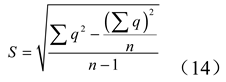
The target spraying device was integrated into a 3WPZ-200 self-propelled electric boom sprayer and comprised four main subsystems: an image acquisition unit, a pesticide supply unit, a spray execution unit, and a traveling system, as shown in Figure 1. The image acquisition unit was responsible for real-time field image collection, while the pesticide supply and spray execution units cooperatively enabled precise pesticide delivery. The traveling system provided stable forward motion during field operations.
The image acquisition unit consisted of two cameras (MV-CA016, Hangzhou Hikvision Digital Technology Co., Ltd., China) and an onboard computer (Intel NUC, Intel Corporation, USA) equipped with an Intel i7-1165G7 CPU, an NVIDIA GTX 2060 GPU with 6 GB memory, and 16 GB RAM. The cameras, each with a resolution of 1440 × 1080 pixels and equipped with a 4 mm focal-length lens, were used to acquire field images. To ensure full coverage of the spray boom, the two cameras were mounted symmetrically at one-quarter and three-quarters of the boom length on the left and right sides, respectively, with each camera responsible for monitoring half of the operating area. The cameras were installed at a height of 0.5 m above the spray boom. The onboard computer received the video streams captured by the cameras, executed deep learning–based target detection and precision target spraying strategy in real time, and transmitted control commands to the controller via serial communication.
The pesticide supply unit mainly consisted of a pesticide tank, a filter (Kaiping WOEN Sanitary Ware Co., Ltd., China), a pump (Dafengda 5G-210, China), a buffer tank (TY-11-0.5G-5, Taizhou Tianyang ElectricalCo., Ltd., China), a flow sensor (Shanghai Weill Instrument Co., Ltd., China), and a pressure sensor (MIK-P300, Hangzhou MEACON Automation Technology Co., Ltd., China). The filter was installed upstream of the pump to remove impurities from the pesticide solution. The pump was used to pressurize the spray liquid and deliver it to the nozzles for atomization. The buffer tank was used to attenuate pressure fluctuations in the liquid flow, thereby ensuring stable spray pressure. The flow sensor was used to measure the real-time flow rate in the pipeline. The pressure sensor was used to monitor the pressure of the spraying system in the range of 0–1.0 MPa, with a measurement accuracy of 0.005 MPa.
The spray execution unit comprised a controller, solenoid valves (2V025, AirTAC International Group,China), MOSFET-based valve driver circuits, an incremental encoder (E6B2-CWZ3E, VEHA Corporation, China), and nozzles (model 2501, Dongguan Wuyuan Spraying and Purification Technology Co., Ltd., China). The controller was based on an STM32F103ZET6 microcontroller (Guangzhou Xingyi Electronic Technology Co., Ltd., Guangzhou, China). The solenoid valve controlled the opening and closing of the nozzle at a voltage of DC 24 V and a pressure range of 0–1.0 MPa, with a maximum switching frequency of 10 Hz. In the de-energized state, the solenoid valve remained closed under the action of the spring. When the solenoid coil was energized, the valve core was rapidly attracted, switching the valve to the open state and enabling spray on-off operation. The MOSFET-based valve driver circuits converted the control signals from the controller into driving signals for the solenoid valves. The incremental encoder was used to measure the forward speed of the sprayer. Flat-fan stainless-steel nozzles with a spray angle of 25° were employed, with a nozzle spacing of 15 cm. When the solenoid valves were activated, the pesticide solution flowed through the nozzle, enabling precision target spraying.
The traveling unit consisted of a liftable spray boom, chassis, steering system, battery (60 V), and drive motors. A four-wheel steering mode was adopted to enhance maneuverability under field conditions. The spray boom had a working width of 3 m. Detailed technical parameters of the sprayer are summarized in Table 1.
During operation, the cameras capture field images and transmit them to the onboard computer. The computer preprocesses the images and performs target detection using a pre-trained deep learning model. Based on the detection results, decisions are made regarding the opening and closing of the solenoid valve assembly. These control signals are transmitted in real time to the spray execution unit via serial communication as data frames. The controller of the spray execution unit parses the data frames, sets the corresponding control pins to the low or high level, and, after processing by the valve driver circuit, actuates the solenoid valves. Consequently, the pesticide solution is sprayed from the nozzles, enabling precision target spraying. Meanwhile, the buffer tank of the pesticide supply unit mitigates pressure fluctuations in the pipeline caused by intermittent spraying, maintaining a constant supply pressure and ensuring stable nozzle atomization quality. The schematic diagram of the main components of the target spraying system is shown in Figure 2.
2.2. Weed detection Method
2.2.1. Image Acquisition
Field image data were collected at three locations in Henan Province in July 2022: Yuan Zhuang Village, Suixian County (34.136°N, 115.343°E); Zhou Zhuang Village, Linying County (33.774°N, 113.837°E); and the experimental field at the Changyuan Branch of the Henan Academy of Agricultural Sciences (35.428°N, 114.289°E). The images were captured using a smartphone (Redmi K30 Pro, Xiaomi Corporation, China) in JPEG format with a resolution of 1440 × 1080 pixels, as shown in Figure 3a. The weed species collected was Cirsium setosum (also known as Cirsium arvense var. integrifolium, Figure 3b). The dataset included images taken under various weather conditions, such as sunny, cloudy, and post-rain, as well as different land backgrounds, including bare soil and wheat stubble fields. These images exhibit diversity in environmental lighting and background conditions, which enhances the generalization ability of the trained model.
2.2.2. Data Augmentation
To improve the generalization ability of the model, data augmentation was applied to increase the diversity and size of the original dataset [47]. Mosaic online data augmentation was employed during model training. This technique involves randomly cropping and concatenating multiple images to create a new training sample, referred to as a mosaic sample, which contains multiple objects and backgrounds. During training, the model learns to detect and classify these different targets while distinguishing their relationships with the background. Mosaic augmentation also reduces dependence on the training data, mitigates the risk of overfitting, and improves model performance. Weed-labeled images after mosaic augmentation are shown in Figure 4.
In this study, a total of 3200 images were annotated using the CVAT image annotation tool. The annotated dataset was then randomly divided into training, validation, and test sets at a ratio of 7:1:2, resulting in 2,240 images for the training set, 320 images for the validation set, and 640 images for the test set. These subsets were subsequently used for model training and evaluation.
2.2.3. Weed Detection Model Based on YOLOv5-MobileNetv3-SE
This study is based on the YOLOv5 object detection algorithm. The extensive convolutional operations in the CSPDarknet backbone of YOLOv5 require substantial computational resources and time, which makes it unsuitable for deployment on resource-constrained edge devices [48]. To improve efficiency, the model was lightweighted by replacing the CSPDarknet backbone with the more lightweight MobileNetV3 model, reducing computational load and model size. Additionally, given the complexity of field images and the small size of some weed targets, which may lead to misdetections or missed detections, an SE (Squeeze-and-Excitation) attention module was added after each of the three output layers of the backbone network. The attention mechanism, similar to human visual selective attention, selects the most relevant information for the task, suppresses irrelevant data, and increases the weight of useful features. This enables the network to automatically learn and improve computational efficiency, enhance the weight of effective feature channels, and focus on important features, ultimately improving the accuracy of small-target weed detection. The network takes 640 × 640 RGB images as input, and its output consists of three tensors of different sizes: 80 × 80 × 255, 40 × 40 × 255, and 20 × 20 × 255. The Architecture of the improved model is shown in Figure 5.
2.2.4. Model Training and Parameter Settings
The hardware environment used for model training in this study consists of an NVIDIA GeForce RTX 3090 GPU with 24GB of VRAM, an Intel® Core™ i9-12900K processor, and 64GB of RAM. The software environment includes the Windows 10 operating system, Python 3.7, PyTorch 11.7.1, CUDA 11.5, and PyCharm 2020. The input image size was set to 640×640, with padding applied to maintain the original aspect ratio. The initial learning rate was set to 0.1, and a cosine annealing schedule was used during training. The Adam optimizer was employed for model optimization, and the model was trained for 300 epochs. Model convergence was assessed by monitoring the loss value during training and the variation of mAP curves on the validation set. Once convergence was achieved, the weights corresponding to the lowest loss in the final training epochs were selected as the trained model.
2.3. Precision Target Spraying Strategy
Based on the weed detection results obtained by the proposed YOLOv5-MobileNetv3-SE model, a precision target spraying strategy was developed to achieve accurate synchronization between target position and spray actuation. The overall strategy consisted of a grid-based matching spraying algorithm, system time delay analysis, and a time-delay compensation method.
2.3.1. Grid-Based Matching Spraying Algorithm
Line-crossing detection algorithms have been widely used in applications such as video surveillance and traffic safety, where targets are identified by determining whether they cross predefined virtual lines, enabling effective monitoring and management of designated regions [49,50]. Based on this concept, an improved grid- based matching spraying algorithm was proposed in this study. The algorithm established a correspondence between the targets detected by the image acquisition unit and the spray nozzles mounted on the boom, thereby determining which nozzles should be activated and when they should be triggered. Based on this matching relationship, control data frames for the solenoid valve array were generated and transmitted to implement an on–off control strategy, whereby each solenoid valve was switched on or off according to the algorithm decision results. This enabled precise regulation of solenoid valve opening and closing, ultimately achieving accurate target spraying.
The specific implementation of the proposed algorithm is illustrated in Figure 6. A series of grids is overlaid on the image plane, where each grid corresponds one-to-one with a solenoid valve on the spray boom. The width of each grid is set equal to the average spray width of a single nozzle, while the grid height is fixed at 60 pixels. During forward operation of the boom sprayer, images move downward in the image frame. The deep learning–based target detection algorithm continuously detects weed targets and generates regions of interest (ROIs), which are represented by red bounding boxes. When an ROI overlaps with a grid, it indicates that the target has entered the spraying area of the corresponding nozzle. The intersection area between each grid and the ROI is calculated. If the intersection area exceeds a predefined threshold, the corresponding grid is assigned a value of 1, indicating that the solenoid valve should be activated for spraying; otherwise, it is assigned a value of 0, indicating that the valve remains closed. In this study, the threshold is set to 20% of the grid area.
Several spatial relationships between ROIs and grids may occur during operation. When the ROI of a single weed intersects with only one grid, a single nozzle is activated. When the ROI intersects with two or more grids, multiple nozzles are activated simultaneously. In cases where multiple weeds overlap spatially, the resulting ROIs intersect multiple grids, and the corresponding solenoid valves are activated accordingly. In addition, due to the inherent opening and closing delays of the solenoid valves during practical operation, if the spacing between adjacent weeds in the forward travel direction is shorter than the valve response time (the yellow region shown in Figure 6),the grid signal is still maintained as 1 to ensure continuous spraying. In this study, each camera is responsible for controlling ten nozzles. Data exchange between the onboard computer and the controller is performed via serial communication.
2.3.2. System Time Delay Analysis
In the above analysis, it is assumed that the grid positions coincide with the locations of the spray boom within the camera field of view. Accordingly, when the intersection area between the ROI and a grid exceeds a predefined threshold, the onboard computer sends an opening signal to the corresponding solenoid valve. However, during actual operation, a certain amount of time is required from the moment the control command is issued by the computer to the moment when pesticide droplets are deposited on the weeds. This time delay causes a longitudinal offset between the actual spraying region and the target spraying region, resulting in missed spraying region in precision target spraying application, as illustrated in Figure 7.
Further analysis indicates that the total system time delay in the target spraying process mainly consists of three components: image processing delay, communication and control delay, and spray deposition delay. Therefore, it is necessary to quantitatively measure each delay component through dedicated experiments to determine the overall system latency. The resulting total delay can then be used to compensate for the spraying lag by adjusting the spatial offset distance, thereby reducing spray omission and improving target spraying accuracy.
- Image processing delay
The image processing delay mainly originated from the inference time required by the deep learning–based weed detection model. Although the target detection model was lightweighted in this study to reduce computational complexity, the delay introduced by image processing remained non-negligible. To quantify the image processing delay, the trained detection model was deployed on the onboard computer. A total of 200 field-acquired images were processed using weed detection model based on YOLOv5-MobileNetv3-SE. The total inference time was measured as 5.58 s, corresponding to an average processing time of 27.9 ms per image.
- 2.
- Communication and control delay
The communication and control delay referred to the time consumed from the moment when the onboard computer transmitted a control command to the moment when the microcontroller decoded the data frame, set the corresponding control pins, and output the driving voltage through the solenoid valve driver circuit to actuate the solenoid valve. To measure the communication and control delay, a single-channel solenoid valve control setup was constructed, consisting of a microcontroller, a solenoid valve driver board, and a solenoid valve, as shown in Figure 8. A valve-opening command was transmitted from the onboard computer using serial communication debugging software to trigger the opening of the solenoid valve. Meanwhile, a digital oscilloscope (TBS1102C, Tektronix, Inc., USA) was used to monitor the signals. One channel of the oscilloscope was connected to the serial input pin of the microcontroller, while the other channel was connected to the output terminal of the solenoid valve driver board. By capturing and comparing the waveforms from the two channels, the time difference between the input control signal and the output driving voltage was determined. The results showed that the time interval from the reception of the first pulse signal at the microcontroller serial port to the output of the 24 V driving voltage by the solenoid valve driver board was 6.37 ms.
- 3.
- Spray Deposition Delay
The spray deposition delay referred to the time interval from the moment when the solenoid valve received the driving signal from the driver board and initiated opening to the moment when the pressurized pesticide was atomized through the nozzle, traveled through the air, and finally deposited onto the weed. In this study, the spray process was captured using a high-speed camera, and the deposition delay was determined through frame-by-frame image analysis, as shown in Figure 9. The high-speed camera operated at a frame rate of 960 frames per second, corresponding to a temporal resolution of 1.04 ms per frame. To accurately determine the initial moment when the solenoid valve was energized, a green indicator light was installed above the solenoid valve. The indicator illuminated simultaneously with valve energization and turned off when the power was cut, thereby serving as a reference for the timing of valve coil energization and de-energization. A container filled with water dyed with carmine was placed beneath the nozzle. When spray droplets reached the water surface, visible surface disturbances were generated, which were used to identify the moment when the droplets arrived at the target surface.
During the experiment, the spray pressure was set to 0.3 MPa, and the nozzle height above the ground was 50 cm. The solenoid valve was briefly energized to generate a single intermittent spraying event. The spraying process was recorded using a high-speed camera, and the corresponding image frames are shown in Figure 10. The spraying sequence was divided into six key stages: signal onset, spray initiation, droplet arrival at the ground, continuous spraying, signal termination, and spray termination. The frame in which the indicator light switched from off to on was defined as frame 0. Spray droplets were first observed emerging from the nozzle at frame 6. At frame 35, visible ripples appeared on the water surface in the collection tray placed on the ground, indicating that the droplets had reached the ground surface. Continuous spraying was maintained until frame 43, when the indicator light began to turn off. Subsequently, the ripples on the water surface gradually weakened and nearly disappeared by frame 90, marking the end of the intermittent spraying event. Based on the frame intervals, the elapsed time from the indicator light turning on to the initial droplet ejection was approximately 6.24 ms, while the droplet travel time from the nozzle to the ground was approximately 36.40 ms. After the control signal was terminated at 44.72 ms, spraying continued until 93.60 ms, resulting in a solenoid valve closing delay of 48.88 ms from the open to the closed state. Therefore, the spray deposition delay was determined to be 36.40 ms.
Based on the above experimental measurements, the total system time delay of the precision target spraying system was determined to be 70.67 ms.
2.3.3. Time-delay compensation method
In the camera field of view, the grid position determines the triggering timing of the solenoid valves. As discussed above, when the grid position coincides with the actual spray boom position, an overlap between the grid and the ROI leads to mistimed spraying due to system time delay, resulting in spray misalignment or missed spraying. Therefore, advancing the grid position relative to the spray boom to trigger the solenoid valve earlier effectively compensates for the system time delay, thereby reducing spray omission and improving the precision of target spraying. A schematic illustration of the time-delay compensation method is shown in Figure 11. A planar coordinate system XOY is established, in which the center of the camera field of view is defined as the X-axis and the forward traveling direction of the sprayer is defined as the Y-axis. The distance between the nozzle and the camera along the forward direction is denoted as e. When the target spraying system is stationary, the grid centerline L₂ coincides with the spray centerline L₁, ensuring that the pesticide droplets accurately deposit onto the target. During forward operation, the grid is shifted upward in the image by a certain distance, allowing the predicted bounding box to intersect the grid earlier and thereby compensating for the system delay. Consequently, the relative distance g between the matching grid centerline L₂ and the Y-axis in the world coordinate system can be expressed as:
where d is the distance between the grid centerline and the spray centerline (m). The distance e represents the separation between the nozzle and the camera along the forward traveling direction (m), which was set to 0.1 m in this study.
The value of d is determined by the system delay time and the forward speed of the sprayer.
where v is the real-time forward speed of the sprayer (m·s−1), and t represents the totol delay time (s). Based on the above experimental measurements, t was determined to be 76 ms. The real-time forward speed of the sprayer was obtained using an incremental encoder. Accordingly, the grid position in the image is dynamically adjusted according to the sprayer speed to advance the opening timing of the solenoid valves, thereby achieving accurate alignment between the spray deposition area and the target region.
To implement the grid-based matching algorithm, the compensated grid position is first transformed from the world coordinate system to the pixel coordinate system. Subsequently, an intersection calculation is performed between the transformed grid and the pixel coordinates of the ROI obtained from target detection. The grid state (1 or 0) is then determined to control the opening and closing of the corresponding solenoid valves. Through this dynamic grid adjustment strategy, accurate alignment between the spray deposition area and the target spraying region is achieved. The world coordinate system is a three-dimensional Cartesian coordinate system used to describe the spatial relationship between the camera and observed objects, whereas the pixel coordinate system is defined on the image plane output by the camera and is used to represent pixel locations in the image. In this study, the world coordinate system is denoted as OXYZ, where the Z-axis points toward the camera viewing direction, the X-axis points to the right side of the image, and the Y-axis points downward, as shown in Figure 12. A spatial point P in the world coordinate system is represented as [X, Y, Z]T. The pixel coordinate system corresponding to the camera imaging process is denoted as ouv, with the origin o located at the upper-left corner of the image. The u-axis is parallel to the X-axis, and the v-axis is parallel to the Y-axis. Accordingly, the pixel coordinates of point P on the image plane can be expressed as p[u,v]T.
According to the pinhole camera model, the relationship between the world coordinate system and the pixel coordinate system can be expressed as follows:
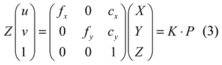
Here, the matrix composed of the intermediate parameters represents the intrinsic parameter matrix K of the camera. In this study, the camera was calibrated using Zhang’s calibration method. The camera is mounted above and slightly ahead of the spray nozzle. The width of the field of view on the ground is related to the lens viewing angle and the installation height, as described below.
Where h1 is the installation height of the spray nozzle (m) and h2 is the installation height of the camera relative to the nozzle (m). In this study, the nozzle installation height was set to 0.5 m, and the camera was mounted 0.5 m above the nozzle. Consequently, the pixel coordinates of point p in the image plane can be obtained.
The above analysis is mainly aims to ensure that the onset of the actual spraying region coincides with that of the target spraying region. High-speed camera observations of the spraying process indicate that, after the stop signal is issued, spray droplets continue to be discharged for a short duration before completely ceasing, resulting in overspray at the end of the spraying operation, as illustrated in Figure 13. Therefore, to ensure that the termination of spraying accurately coincides with the target area, the stop signal must be issued in advance during the fitting of the weed prediction bounding box, as shown in Figure 7a. Accordingly, the length L of the actual target spraying region can be expressed as:
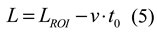
where LROI is the length of the ROI fitted by the deep learning–based detection algorithm after target recognition, and t0 is the time interval from the issuance of the stop signal to the complete cessation of spraying, measured as 48.88 ms (Figure 10). With this advance stopping strategy, the termination position of the actual spraying precisely coincides with the target spraying region.
The overall control flow chart of the target spraying system is illustrated in Figure 14.
2.4. Evaluation Experiments
An experimental evaluation of the target spraying system was conducted using both laboratory and field experiments. The laboratory experiments primarily assessed model recognition performance, target spraying accuracy, pesticide reduction rate, and spray distribution uniformity. The laboratory test platform, shown in Figure 15, consisted of a rail system, a power supply module, an electric rail vehicle, and the target spraying system. The platform had a maximum load capacity of 150 kg, a maximum forward speed of 8 km·h⁻1, and an adjustable spray boom height ranging from 0 to 120 cm.
2.4.1. Model Detection Performance
An experimental evaluation was conducted to assess the weed recognition performance of the trained YOLOv5-MobileNetv3-SE model. The evaluation metrics included precision (P), recall (R), and mean average precision at 0.5 intersection over union (mAP@0.5), model size, and frames per second (FPS).
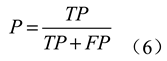
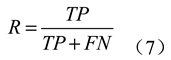
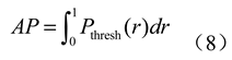
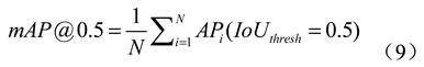
Where TP is true positive; FP is false positive; TN is true negative; FN is false negative.
To further evaluate the performance of the proposed model, comparative experiments were conducted with several classical deep learning–based detection models, including Faster R-CNN, YOLOv3, YOLOv5s, and YOLOv5x. All models were trained under identical conditions and evaluated on the same test platform using the same dataset.
2.4.2. Target Spraying Accuracy
The laboratory test for target spraying accuracy is illustrated in Figure 16. Considering the acceleration and deceleration phases of the electric rail vehicle, the first and last 2 m of the track were excluded, and only the central 8 m section with constant speed was used for testing. The width of the test area was 1.2 m. To facilitate the experiments, plastic weed models were used to replace real weeds. Each plastic weed model was approximated as a circular projection on the ground with a diameter of 0.12 m, corresponding to a single-weed coverage area of 0.0113 m2. With a weed coverage rate of 10%, a total of 85 plastic weed models were randomly distributed within the test area. Additionally, three rows of plastic soybean models (60 plants in total) were uniformly arranged as interference objects, with both row spacing and plant spacing set to 0.5 m. To determine whether spray droplets reached the weeds, a 2 cm × 2 cm water-sensitive paper was attached to the leaf of each plastic weed model. During the experiment, the forward speed of the electric rail vehicle was set to 1, 2, 3, and 4 km/h. The experimental metrics include weed detection accuracy rate (WDAR) and spraying accuracy rate (SAR).
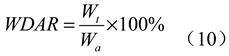
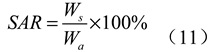
where Wa is the total number of weeds in the test area, Wt is the actual number of detected weeds, Ws the number of weeds effectively sprayed. Detection accuracy was determined by the appearance of a purple bounding box around the weed (Figure 16). For spraying accuracy, if the actual spray length covered at least 60% of the target spray length, the weed was considered successfully sprayed (Figure 13b).
2.4.3. Pesticide Reduction Rate
Precision target spraying can effectively reduce pesticide consumption compared to conventional full-coverage spraying. In this study, the pesticide reduction rate of target spraying under different weed coverage levels was evaluated by comparing it with conventional continuous spraying. Weed coverage is an important factor influencing the pesticide reduction rate. To simulate different weed coverage scenarios, plastic weed models were used instead of real weeds. Each plastic weed model had an approximately circular ground projection with a diameter of 0.12 m, corresponding to an area of approximately 0.0113 m2. Four simulated field environments with weed coverage rates of 5%, 10%, 15%, and 20% were established within a test area of 1.2 m × 5 m, corresponding to 13, 27, 53, and 106 weed models, respectively. The plastic weed models were randomly distributed within the experimental area. Water was used in the pesticide tank instead of actual pesticide, and target spraying experiments were conducted on the precision spraying test platform at a forward speed of 2 km/h. For each weed coverage level, 30 experimental runs were performed. Additionally, a control group was tested using conventional continuous spraying, in which all solenoid valves remained fully open, also repeated 30 times. After each test, the remaining liquid volume in the pesticide tank was recorded. The pesticide reduction rate S was calculated as the percentage reduction in liquid consumption achieved by precision target spraying compared with conventional continuous spraying:
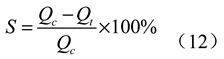
where Qc and Qt are the pesticide consumption under conventional continuous spraying and precision target spraying, respectively.
2.4.4. Spray Distribution Uniformity
The uniformity of pesticide droplet distribution directly affects the efficacy of pesticide application. The target spraying system is an upgraded version of traditional sprayers, retaining compatibility with conventional full-coverage spraying. In target spraying mode, ensuring even droplet distribution is crucial for optimal application effectiveness. Therefore, a droplet distribution scanner (SALVARANI, AAMS Co., Ltd., Belgium), as shown in Figure 17, was used to measure spray distribution uniformity. Each collecting channel of the scanner had a width of 10 cm, and a standard graduated cylinder equipped with a liquid level sensor was installed beneath each channel. The filling time of each cylinder was automatically recorded, enabling determination of the spray flow rate for each channel. The scanner was mounted on a motor-driven rail, allowing lateral movement beneath the spray boom to measure the overall transverse distribution of the spray volume.
The experiment was conducted in accordance with the requirements of the national standard GB/T 24677.1–2009, China. Water was used as the test medium, and the measurements were performed at a pressure of 0.3 MPa, a nozzle spacing of 15 cm, and a nozzle height of 50 cm above the ground. The coefficient of variation (CV) was employed to evaluate the spray distribution uniformity. A lower CV value indicates a more uniform distribution of spray volume along the boom.
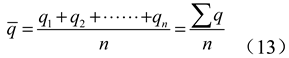
where qi is the spray flow rate of the ith nozzle (L/min); n is the number of nozzles;  is the average spray flow rate (L/min);
  is the total spray flow rate of the sprayer (L/min); S is the standard deviation(L/min). After three repeated tests, the CV of the nozzles was 5.9%. This value satisfies the requirement specified in GB/T 24677.1–2009, which stipulates that the CV of spray volume distribution should be less than 20%.
is the average spray flow rate (L/min); is the total spray flow rate of the sprayer (L/min); S is the standard deviation(L/min). After three repeated tests, the CV of the nozzles was 5.9%. This value satisfies the requirement specified in GB/T 24677.1–2009, which stipulates that the CV of spray volume distribution should be less than 20%.
2.4.5. Field Performance of Precision Target Spraying
To verify the field performance of the precision target spraying system, field experiments were conducted in Suixian City, Henan Province, China (34.136°N, 115.343°E). Three rectangular plots, each measuring 20 m × 3 m, were delineated within the experimental field as sampling areas. The number of weeds and the dimensions of their bounding rectangles within each plot were recorded. Precision target spraying trials were conducted at forward speeds of 2, 3, and 4 km/h. The field experimental setup and spraying process are shown in Figure 18.
A 2 cm × 2 cm water-sensitive paper was affixed to the leaves of each weed. The paper changed color to red upon contact with spray droplets, allowing verification of whether the pesticide effectively reached the target, as shown in Figure 19. The weed detection accuracy rate and spraying accuracy rate were then calculated using Equations (10) and (11), respectively.
3. Results and Discussion
3.1. Model Detection Performance
The detection results of different models are summarized in Table 2. The mAP@0.5 of YOLOv5-MobileNet-SE was 86.9%, which is slightly lower than YOLOv3, YOLOv5s, and YOLOv5x by 0.9% 0.7%, and 1.3%, respectively, while outperforming Faster R-CNN by 6.0%. The model size of YOLOv5-MobileNet-SE was 7.5 MB, which is 46.4%, 95.6%, 93.8%, and 93.2% smaller than YOLOv5s, YOLOv5x, YOLOv3, and Faster R-CNN, respectively. The FPS of YOLOv5-MobileNet-SE was 38.17, which is 1355.2%, 46.5%, 27.7%, and 68.6% higher than YOLOv5s, YOLOv5x, YOLOv3, and Faster R-CNN, respectively. These results indicate that the proposed YOLOv5-MobileNet-SE model significantly reduces model complexity and improves real-time performance while incurring only a marginal loss in detection accuracy. Overall, the model exhibits superior comprehensive performance and satisfies the real-time and lightweight requirements of precision target spraying applications.
There are several deployment strategies for deep learning models, including local deployment, cloud-based deployment, and hybrid deployment approaches [51]. In this study, the trained model was deployed on the local onboard computer of the sprayer using TensorRT. TensorRT is a high-performance inference engine developed by NVIDIA that exploits GPU parallel computing to automatically optimize deep learning models through techniques such as layer fusion, weight compression, and quantization, thereby significantly accelerating the inference process. The improved YOLOv5-MobileNetv3-SE model was first converted into the ONNX format using the conversion scripts provided by the YOLOv5 framework. Subsequently, the ONNX model was converted into a TensorRT engine file, enabling efficient inference on the onboard computer.
3.2. Target Spraying Accuracy
The target spraying accuracy results are shown in Table 3. The weed detection accuracy rates were 98.88%, 97.64%, 94.11%, and 92.94% at forward speeds of 1, 2, 3, and 4 km/h, respectively. At higher speeds, the time available for the model to detect and classify weeds was reduced, resulting in lower recognition accuracy because the model had less time to process each frame and make precise predictions. Additionally, higher speeds could introduce motion blur or reduced image resolution, further impairing the model’s ability to accurately identify weeds. The target spraying accuracy rates were 97.64%, 95.29%, 90.58%, and 85.88% at forward speeds of 1, 2, 3, and 4 km/h, respectively, showing a clear downward trend as speed increased. This reduction in spraying accuracy can be attributed to two main factors. First, the decrease in weed detection accuracy at higher speeds led to fewer weeds being correctly detected and sprayed. Second, the increased forward speed negatively affected the precision target spraying strategy, causing deviations in droplet deposition and occasional off-target spraying.
3.3. Pesticide Reduction Rate
The pesticide reduction rates for precision target spraying and conventional continuous spraying under different weed coverage levels are presented in Table 4. The results indicate that precision target spraying achieved pesticide savings of 79.0%, 72.5%, 55.8%, and 48.6% at weed coverage rates of 5%, 10%, 15%, and 20%, respectively. As the weed coverage rate decreased, the pesticide-saving effect of precision target spraying became more pronounced, which aligns with the intended design of the system. The corresponding relative pesticide application rates of target spraying compared with continuous spraying were reduced to21.0%, 27.5%, 44.2%, and 51.4% at weed coverage rates of 5%, 10%, 15%, and 20%, respectively. In all cases, the relative pesticide application rates exceeded the corresponding weed coverage rates. This is attributable to the system design, in which the spray coverage area was deliberately set larger than the ground-projected area of individual weeds to ensure complete droplet deposition on the targets (Figure 6). Overall, the experimental results demonstrate that precision target spraying can substantially reduce pesticide usage compared with conventional continuous spraying, particularly under conditions of low weed coverage.
3.4. Field Performance Of Precision Target Spraying
The field test results of the precision target spraying system are summarized in Table 5. The weed detection accuracy rates were 95.40%, 92.41%, and 86.40% at forward speeds of 2, 3, and 4 km/h, respectively, which decreases with increasing speed. As the forward speed increased from 2 km/h to 4 km/h, the weed detection accuracy rate decreased by 9%. The field test results showed a reduction in weed detection accuracy rate compared to the laboratory tests, with decreases of 2.29%, 1.81%, and 7.04%, respectively. The spraying accuracy rates were 90.80%, 86.20%, and 79.61% at forward speeds of 2, 3, and 4 km/h, respectively, corresponding to decreases of 4.95%, 5.08%, and 7.87% relative to the laboratory experiments. These reductions in both detection and spraying accuracy can be attributed to several factors. Uneven field terrain combined with increased forward speed resulted in enhanced vibrations of the sprayer, which degraded image capture quality and reduced effective detection rates. The vibrations also amplified nozzle movements on the spray boom, causing misalignment between the nozzle and the target, thereby lowering spraying accuracy. Additionally, environmental factors such as variations in lighting, background interference, and differences in weed appearance, along with motion blur and reduced image resolution at higher speeds, further affected the model's detection performance.
4. Conclusions
This paper proposes a deep learning-based precision target spraying method for weed control in soybean fields, and develops a grid-based matching spraying algorithm to synchronize target detection with spray actuation. Based on the detection model YOLOv5, a lightweight YOLOv5-MobileNetv3-SE model was designed by replacing the backbone feature extraction network and adding an attention mechanism. The improved model achieves an mAP@0.5 of 86.9%, a model size of 7.5 MB, and a frame rate of 38.17 frames per second. Compared to the original YOLOv5s model, the improved model reduced the size to 53.5% of the original while increasing the frame rate by 27.8%, with only minimal loss in detection accuracy. The laboratory test platform and prototype of the target spraying device were employed to evaluate the model detection performance, target spraying accuracy, pesticide reduction rate, and spray distribution uniformity. Laboratory results indicated that, within a forward speed range of 1–4 km/h, the weed detection accuracy exceeded 92.94%, and the spraying accuracy exceeded 85.88%, meeting the precision target requirements. Pesticide reduction tests demonstrated that target spraying achieved pesticide saving rates of 79.0%, 72.5%, 55.8%, and 48.6% at weed coverage rates of 5%, 10%, 15%, and 20%, respectively, with greater savings observed under lower weed coverage, consistent with the design expectations of the system. Spray distribution uniformity tests showed a coefficient of variation of 5.9%, satisfying the national standard GB/T 24677.1–2009. Field experiments further validated the system’s performance, with weed detection accuracy and spraying accuracy exceeding 86.4% and 79.61%, respectively, at forward speeds of 2, 3, and 4 km/h. Overall, these results demonstrate that the proposed method effectively balances model efficiency and detection accuracy, achieving precise spraying while significantly reducing pesticide usage.
Author Contributions
Conceptualization, C.Y., C.G., and Z.H.; methodology, C.Y., Z.Y. and H.L.; formal analysis, C.Y., Q.D. and Z.H.; data curation, C.Y., S.C., and Z.H.; writing—original draft preparation, C.Y. and Z.H.; writing—review and editing, W.W. and H.L. All authors have read and agreed to the published version of the manuscript.
Institutional Review Board Statement
Not applicable.
Data Availability Statement
The data presented in this study are available on request from the first author at yuchang@henau.edu.cn.
Acknowledgments
The authors would like to thank their schools and colleagues as well as those who funded the project. All support and assistance are sincerely appreciated.
Conflicts of Interest
The authors declare no conflicts of interest.
References
- Rotundo, J.L.; Marshall, R.; McCormick, R.; Truong, S.K.; Styles, D.; Gerde, J.A.; Gonzalez-Escobar, E.; Carmo-Silva, E.; Janes-Bassett, V.; Logue, J.; et al. European soybean to benefit people and the environment. Scientific Reports 2024, 14, 7612. [Google Scholar] [CrossRef]
- Messina, M. Perspective: Soybeans Can Help Address the Caloric and Protein Needs of a Growing Global Population. Frontiers in Nutrition 2022, 9, 909464. [Google Scholar] [CrossRef]
- Majidi, M.; Salehian, H.; Rezvani, M.; Dorbeiki, M. Weed flora and wheat yield comparison in conventional (small grain cereals) and organic (soybean-wheat rotation) systems. Journal of Agriculture and Food Research 2025, 24, 102324. [Google Scholar] [CrossRef]
- Schatke, M.; Bensch, J.; Ulber, L.; Gerowitt, B.; Redwitz, C.v. Trait-based weed control decisions compared to economic thresholds for site-specific weed management. European Journal of Agronomy 2026, 174, 127946. [Google Scholar] [CrossRef]
- Zhou, J.; Yang, Y.; Fang, Z.; Liang, J.; Tan, Y.; Liao, C.; Gong, D.; Liu, W.; Liu, G. Trends of pesticide residues in agricultural products in the Chinese market from 2011 to 2020. Journal of Food Composition and Analysis 2023, 122, 105482. [Google Scholar] [CrossRef]
- Faraj, T.K.; EL-Saeid, M.H.; Najim, M.M.M.; Chieb, M.; Faraj, T.K.; EL-Saeid, M.H.; Najim, M.M.M.; Chieb, M. The Impact of Pesticide Residues on Soil Health for Sustainable Vegetable Production in Arid Areas. Separations 2024, 11, 46. [Google Scholar] [CrossRef]
- He, X.; Bonds, J.; Herbst, A.; Langenakens, J. Recent development of unmanned aerial vehicle for plant protection in East Asia. International Journal of Agricultural and Biological Engineering 2017, 10, 18–30. [Google Scholar] [CrossRef]
- Ye, K.; Hu, G.; Tong, Z.; Xu, Y.; Zheng, J.; Ye, K.; Hu, G.; Tong, Z.; Xu, Y.; Zheng, J. Key Intelligent Pesticide Prescription Spraying Technologies for the Control of Pests, Diseases, and Weeds: A Review. Agriculture 2025, 15, 81. [Google Scholar] [CrossRef]
- Teng, H.; Wang, Y.; Chatziparaschis, D.; Karydis, K. Adaptive LiDAR odometry and mapping for autonomous agricultural mobile robots in unmanned farms. Computers and Electronics in Agriculture 2025, 232, 110023. [Google Scholar] [CrossRef]
- Wang, H.; Lin, Y.; Wang, Z.; Yao, Y.; Zhang, Y.; Wu, L. Validation of a low-cost 2D laser scanner in development of a more-affordable mobile terrestrial proximal sensing system for 3D plant structure phenotyping in indoor environment. Computers and Electronics in Agriculture 2017, 140, 180–189. [Google Scholar] [CrossRef]
- Berk, P.; Stajnko, D.; Belsak, A.; Hocevar, M. Digital evaluation of leaf area of an individual tree canopy in the apple orchard using the LIDAR measurement system. Computers and Electronics in Agriculture 2020, 169, 105158. [Google Scholar] [CrossRef]
- Mahmud, M.S.; Zahid, A.; He, L.; Choi, D.; Krawczyk, G.; Zhu, H.; Heinemann, P. Development of a LiDAR-guided section-based tree canopy density measurement system for precision spray applications. Computers and Electronics in Agriculture 2021, 182, 106053. [Google Scholar] [CrossRef]
- Cao, H.L.S.X.S. SGTBN: Generating Dense Depth Maps From Single-Line LiDAR. IEEE Sensors Journal 2021, 21, 19091–19100. [Google Scholar] [CrossRef]
- Zeng, L.; Feng, J.; He, L. Semantic segmentation of sparse 3D point cloud based on geometrical features for trellis-structured apple orchard. Biosystems Engineering 2020, 196, 46–55. [Google Scholar] [CrossRef]
- Palleja, T.; Landers, A.J. Real time canopy density validation using ultrasonic envelope signals and point quadrat analysis. Computers and Electronics in Agriculture 2017, 134, 43–50. [Google Scholar] [CrossRef]
- Zhou, H.; Jia, W.; Li, Y.; Ou, M.; Zhou, H.; Jia, W.; Li, Y.; Ou, M. Method for Estimating Canopy Thickness Using Ultrasonic Sensor Technology. Agriculture 2021, 11, 1011. [Google Scholar] [CrossRef]
- Nan, Y.; Zhang, H.; Zheng, J.; Bian, L.; Li, Y.; Yang, Y.; Zhang, M.; Ge, Y. Estimating leaf area density of Osmanthus trees using ultrasonic sensing. Biosystems Engineering 2019, 186, 60–70. [Google Scholar] [CrossRef]
- Zaman, Q.U.; Esau, T.J.; Schumann, A.W.; Percival, D.C.; Chang, Y.K.; Read, S.M.; Farooque, A.A. Development of prototype automated variable rate sprayer for real-time spot-application of agrochemicals in wild blueberry fields. Computers and Electronics in Agriculture 2011, 76, 175–182. [Google Scholar] [CrossRef]
- Wang, A.; Zhang, W.; Wei, X. A review on weed detection using ground-based machine vision and image processing techniques. Computers and Electronics in Agriculture 2019, 158, 226–240. [Google Scholar] [CrossRef]
- Wang, Y.; Zhang, Z.; Jia, W.; Ou, M.; Dong, X.; Dai, S.; Wang, Y.; Zhang, Z.; Jia, W.; Ou, M.; et al. A Review of Environmental Sensing Technologies for Targeted Spraying in Orchards. Horticulturae 2025, 11, 551. [Google Scholar] [CrossRef]
- Duan, Y.; Han, W.; Guo, P.; Wei, X.; Duan, Y.; Han, W.; Guo, P.; Wei, X. YOLOv8-GDCI: Research on the Phytophthora Blight Detection Method of Different Parts of Chili Based on Improved YOLOv8 Model. Agronomy 2024, 14, 2734. [Google Scholar] [CrossRef]
- Ji, W.; Pan, Y.; Xu, B.; Wang, J.; Ji, W.; Pan, Y.; Xu, B.; Wang, J. A Real-Time Apple Targets Detection Method for Picking Robot Based on ShufflenetV2-YOLOX. Agriculture 2022, 12, 856. [Google Scholar] [CrossRef]
- Zhang, F.; Chen, Z.; Ali, S.; Yang, N.; Fu, S.; Zhang, Y. Multi-class detection of cherry tomatoes using improved Yolov4-tiny model. International Journal of Agricultural and Biological Engineering 2023, 16, 225–231. [Google Scholar] [CrossRef]
- Pei, H.; Sun, Y.; Huang, H.; Zhang, W.; Sheng, J.; Zhang, Z.; Pei, H.; Sun, Y.; Huang, H.; Zhang, W.; et al. Weed Detection in Maize Fields by UAV Images Based on Crop Row Preprocessing and Improved YOLOv4. Agriculture 2022, 12, 975. [Google Scholar] [CrossRef]
- Deng, L.; Miao, Z.; Zhao, X.; Yang, S.; Gao, Y.; Zhai, C.; Zhao, C.; Deng, L.; Miao, Z.; Zhao, X.; et al. HAD-YOLO: An Accurate and Effective Weed Detection Model Based on Improved YOLOV5 Network. Agronomy 2024, 15, 57. [Google Scholar] [CrossRef]
- Zhang, J.; He, L.; Karkee, M.; Zhang, Q.; Zhang, X.; Gao, Z. Branch detection for apple trees trained in fruiting wall architecture using depth features and Regions-Convolutional Neural Network (R-CNN). Computers and Electronics in Agriculture 2018, 155, 386–393. [Google Scholar] [CrossRef]
- Yu, C.; Shi, X.; Luo, W.; Feng, J.; Zheng, Z.; Yorozu, A.; Hu, Y.; Guo, J. MLG-YOLO: A Model for Real-Time Accurate Detection and Localization of Winter Jujube in Complex Structured Orchard Environments. Plant Phenomics 2024, 6, 258. [Google Scholar] [CrossRef]
- Kazmi, W.; Garcia-Ruiz, F.; Nielsen, J.; Rasmussen, J.; Andersen, H.J. Exploiting affine invariant regions and leaf edge shapes for weed detection. Computers and Electronics in Agriculture 2015, 118, 290–299. [Google Scholar] [CrossRef]
- Ahmed, F.; Al-Mamun, H.A.; Bari, A.S.M.H.; Hossain, E.; Kwan, P. Classification of crops and weeds from digital images: A support vector machine approach. Crop Protection 2012, 40, 98–104. [Google Scholar] [CrossRef]
- Zhao, X.; Wang, X.; Li, C.; Fu, H.; Yang, S.; Zhai, C. Cabbage and Weed Identification Based on Machine Learning and Target Spraying System Design. Frontiers in Plant Science 2022, 13, 924973. [Google Scholar] [CrossRef]
- Stachniss, P.L.M.H.S.S.M.M.P.S.L.C. An effective classification system for separating sugar beets and weeds for precision farming applications. IEEE International Conference on Robotics and Automation (ICRA) 2016, 5157–5163. [Google Scholar] [CrossRef]
- Bakhshipour, A.; Jafari, A.; Nassiri, S.M.; Zare, D. Weed segmentation using texture features extracted from wavelet sub-images. Biosystems Engineering 2017, 157, 1–12. [Google Scholar] [CrossRef]
- Min, W.; Wang, Z.; Yang, J.; Liu, C.; Jiang, S. Vision-based fruit recognition via multi-scale attention CNN. Computers and Electronics in Agriculture 2023, 210, 107911. [Google Scholar] [CrossRef]
- Zhang, X.; Wang, Q.; Wang, C.; Wang, X.; Xu, Z.; Lu, C. Guidelines for mechanical weeding: Developing weed control lines through point extraction at maize root zones. Biosystems Engineering 2024, 248, 321–336. [Google Scholar] [CrossRef]
- Chen, J.; Zheng, Y.; Zhang, L.; Wang, M.; Gai, F.; Li, C. The design and implementation of the kernel level mobile storage medium data protection system. IEEE International Conference on Granular Computing (GrC) 2013, 53–57. [Google Scholar] [CrossRef]
- Sun, S.R.K.H.R.G.J. Faster R-CNN: Towards Real-Time Object Detection with Region Proposal Networks. IEEE Transactions on Pattern Analysis and Machine Intelligence 2017, 39, 1137–1149. [Google Scholar] [CrossRef]
- Ross Girshick, J.D., Trevor Darrell, Jitendra Malik. Rich Feature Hierarchies for Accurate Object Detection and Semantic Segmentation. IEEE Conference on Computer Vision and Pattern Recognition 2014, 580–587. [CrossRef]
- Wang, H.; Chen, Y.; Zhang, S.; Guo, P.; Chen, Y.; Hu, G.; Ma, Y. Deep learning-based target spraying control of weeds in wheat fields at tillering stage. Frontiers in Plant Science 2025, 16, 1540722. [Google Scholar] [CrossRef]
- Xu, Y.; Bai, Y.; Fu, D.; Cong, X.; Jing, H.; Liu, Z.; Zhou, Y. Multi-species weed detection and variable spraying system for farmland based on W-YOLOv5. Crop Protection 2024, 182, 106720. [Google Scholar] [CrossRef]
- Rahman, A.; Lu, Y.; Wang, H. Performance evaluation of deep learning object detectors for weed detection for cotton. Smart Agricultural Technology 2023, 3, 100126. [Google Scholar] [CrossRef]
- Rai, N.; Zhang, Y.; Villamil, M.; Howatt, K.; Ostlie, M.; Sun, X. Agricultural weed identification in images and videos by integrating optimized deep learning architecture on an edge computing technology. Computers and Electronics in Agriculture 2024, 216, 108442. [Google Scholar] [CrossRef]
- C, S.G.; Upadhyay, A.; Zhang, Y.; Howatt, K.; Peters, T.; Ostlie, M.; Aderholdt, W.; Sun, X. Field-based multispecies weed and crop detection using ground robots and advanced YOLO models: A data and model-centric approach. Smart Agricultural Technology 2024, 9, 100538. [Google Scholar] [CrossRef]
- Fan, X.; Sun, T.; Chai, X.; Zhou, J. YOLO-WDNet: A lightweight and accurate model for weeds detection in cotton field. Computers and Electronics in Agriculture 2024, 225, 109317. [Google Scholar] [CrossRef]
- He, C.; Wan, F.; Ma, G.; Mou, X.; Zhang, K.; Wu, X.; Huang, X.; He, C.; Wan, F.; Ma, G.; et al. Analysis of the Impact of Different Improvement Methods Based on YOLOV8 for Weed Detection. Agriculture 2024, 14, 674. [Google Scholar] [CrossRef]
- Jiang, W.; Quan, L.; Wei, G.; Chang, C.; Geng, T. A conceptual evaluation of a weed control method with post-damage application of herbicides: A composite intelligent intra-row weeding robot. Soil and Tillage Research 2023, 234, 105837. [Google Scholar] [CrossRef]
- Sunil, G.C.; Upadhyay, A.; Sun, X. Development of software interface for AI-driven weed control in robotic vehicles, with time-based evaluation in indoor and field settings. Smart Agricultural Technology 2024, 9, 100678. [Google Scholar] [CrossRef]
- Shorten, C.; Khoshgoftaar, T.M.; Shorten, C.; Khoshgoftaar, T.M. A survey on Image Data Augmentation for Deep Learning. Journal of Big Data 2019, 6, 1–48. [Google Scholar] [CrossRef]
- Wang, L.; Zhao, Y.; Xiong, Z.; Wang, S.; Li, Y.; Lan, Y. Fast and precise detection of litchi fruits for yield estimation based on the improved YOLOv5 model. Frontiers in Plant Science 2022, 13, 965425. [Google Scholar] [CrossRef]
- HAN, Y.; ZHANG, R.; LU, C.; WANG, G.; HAN, X.; XU, D. Design and Test of Control System for Intelligent Kitchen Waste Treatment Equipment. Transactions of the Chinese Society for Agricultural Machinery 2022, 53, 161–169. [Google Scholar] [CrossRef]
- Azimjonov, J.; Özmen, A.; Varan, M.; Azimjonov, J.; Özmen, A.; Varan, M. A vision-based real-time traffic flow monitoring system for road intersections. Multimedia Tools and Applications 2023, 82 82, 25155–25174. [Google Scholar] [CrossRef]
- Li, J.; Liu, C.; Lu, X.; Wu, B. Fish passage monitoring based on improved YOLO v5s and TensorRT deployment [J]. Transactions of the Chinese Society for Agricultural Machinery 2022, 53, 3–14. [Google Scholar] [CrossRef]
Figure 1.
Overall structure of the target spraying device.
Figure 2.
Schematic diagram of the main components of the target spraying system.
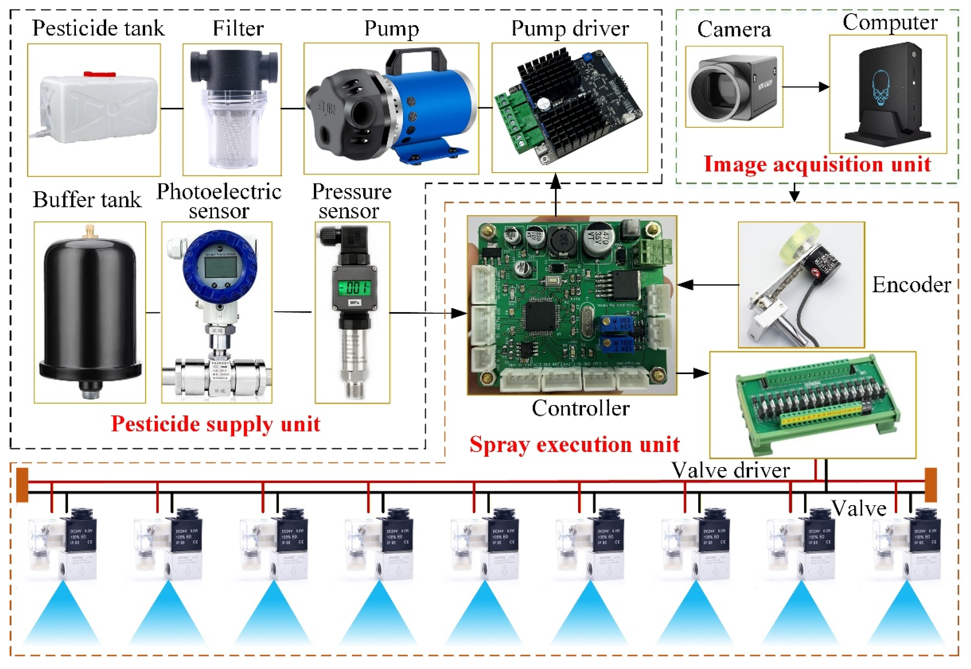
Figure 3.
Image acquisition in the field. (a) Image acquisition process. (b) Target object of image acquisition, Cirsium setosum (also known as Cirsium arvense var. integrifolium).
Figure 3.
Image acquisition in the field. (a) Image acquisition process. (b) Target object of image acquisition, Cirsium setosum (also known as Cirsium arvense var. integrifolium).
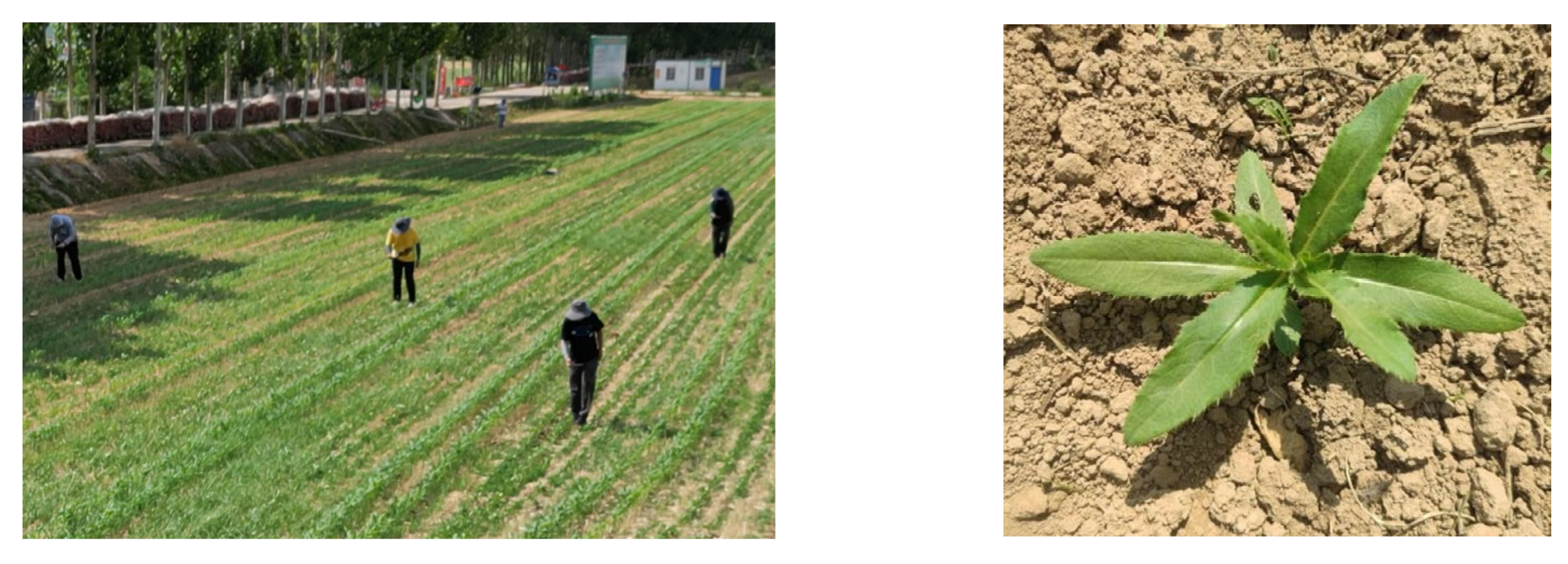
Figure 4.
Images after mosaic augmentation
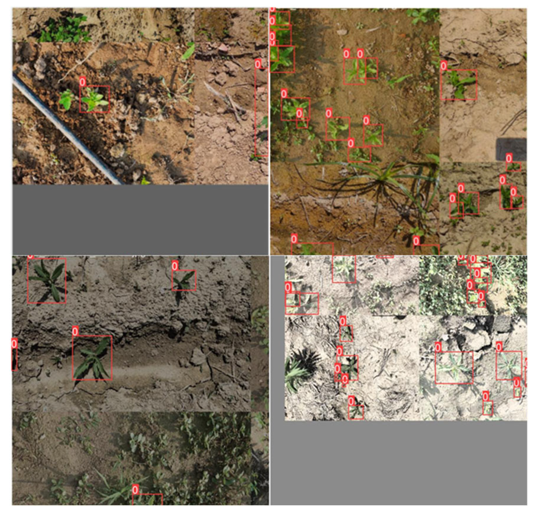
Figure 5.
Figure 5. Architecture of the weed detection model based on YOLOv5-MobileNetv3-SE
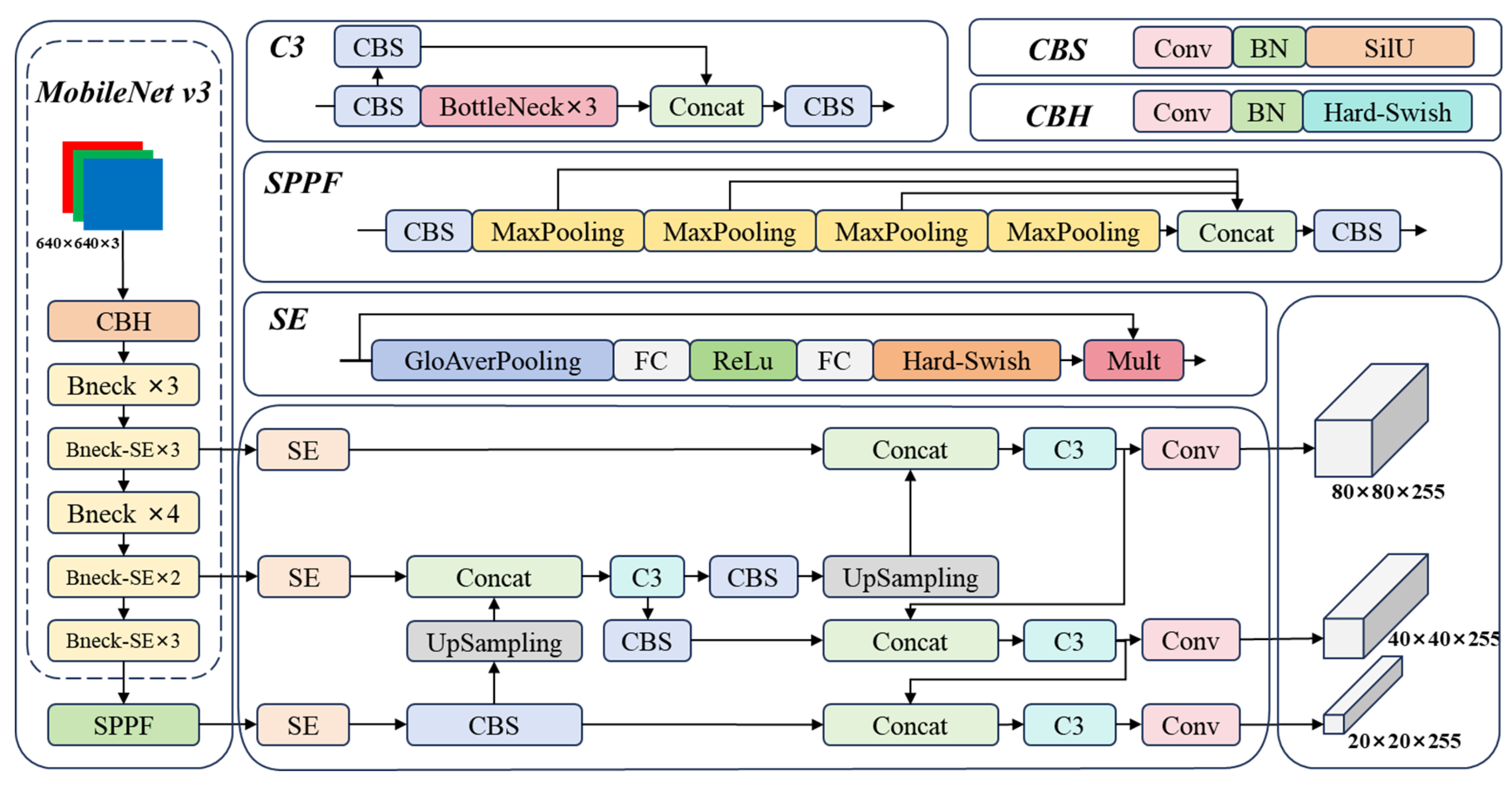
Figure 6.
Figure 6. Schematic diagram of the grid-based matching spraying algorithm
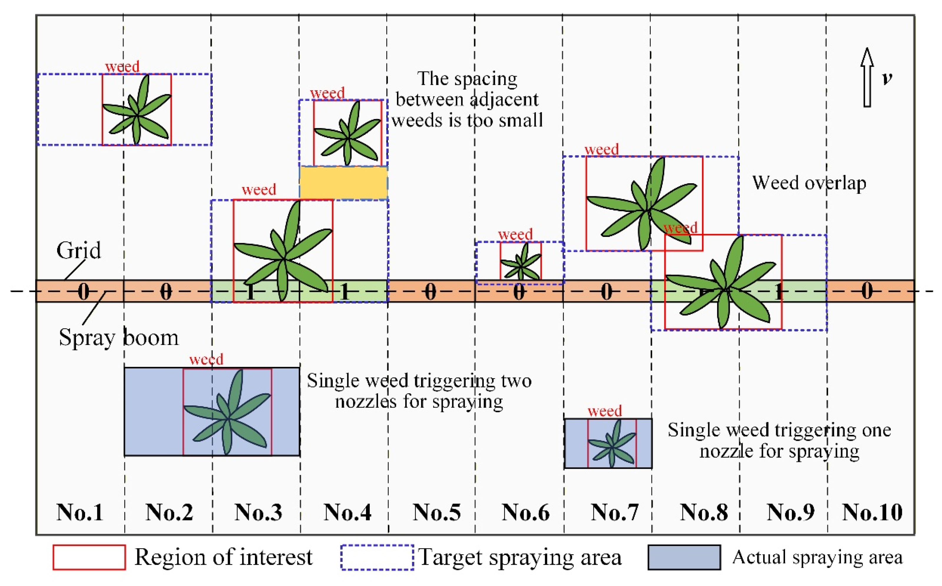
Figure 7.
Spray lag caused by system time delay. (a) Ideal spraying condition, where the actual spraying region coincides with the target spraying region. (b) Spray lag induced by system time delay, resulting in missed spraying region.
Figure 7.
Spray lag caused by system time delay. (a) Ideal spraying condition, where the actual spraying region coincides with the target spraying region. (b) Spray lag induced by system time delay, resulting in missed spraying region.
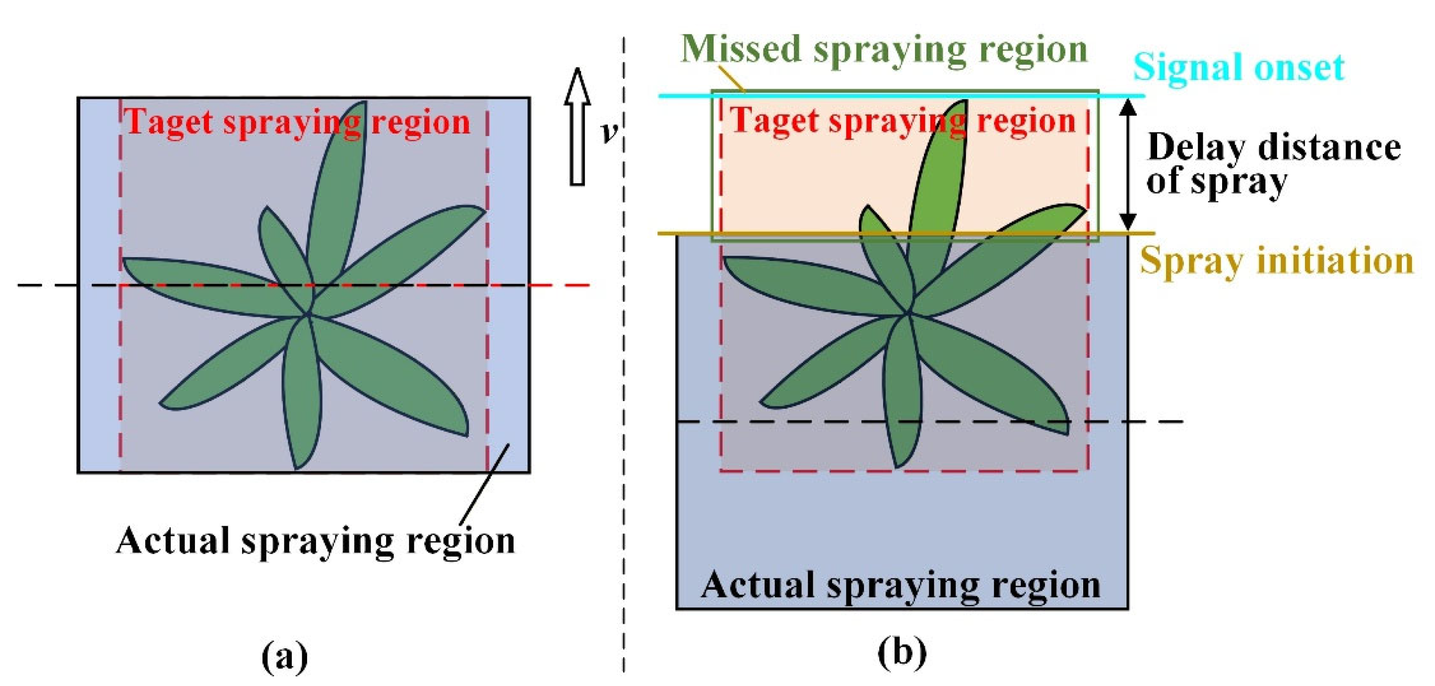
Figure 8.
Measurement of the communication and control delay.
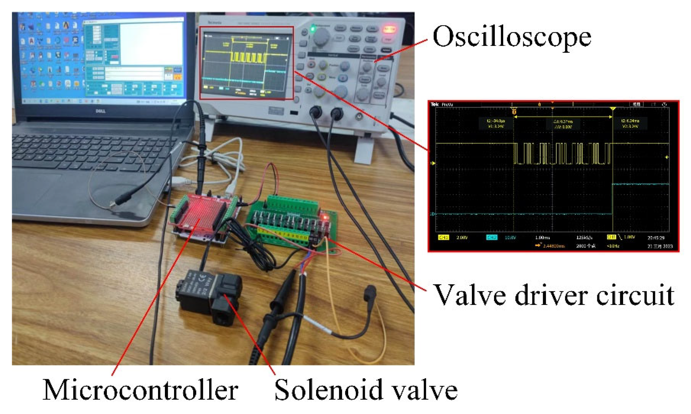
Figure 9.
Measurement of the spray deposition delay.
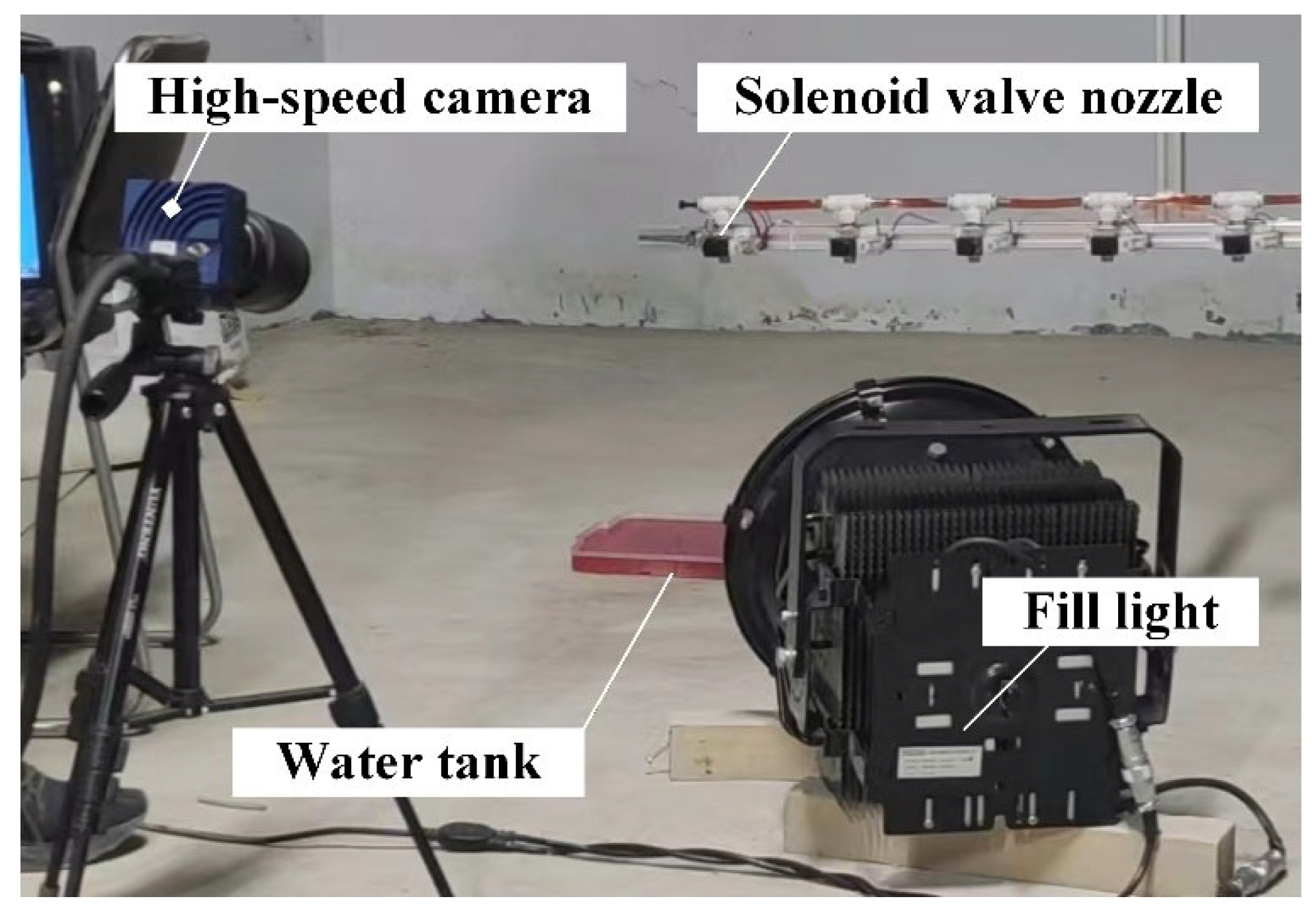
Figure 10.
High-speed camera image sequence of the spraying process.
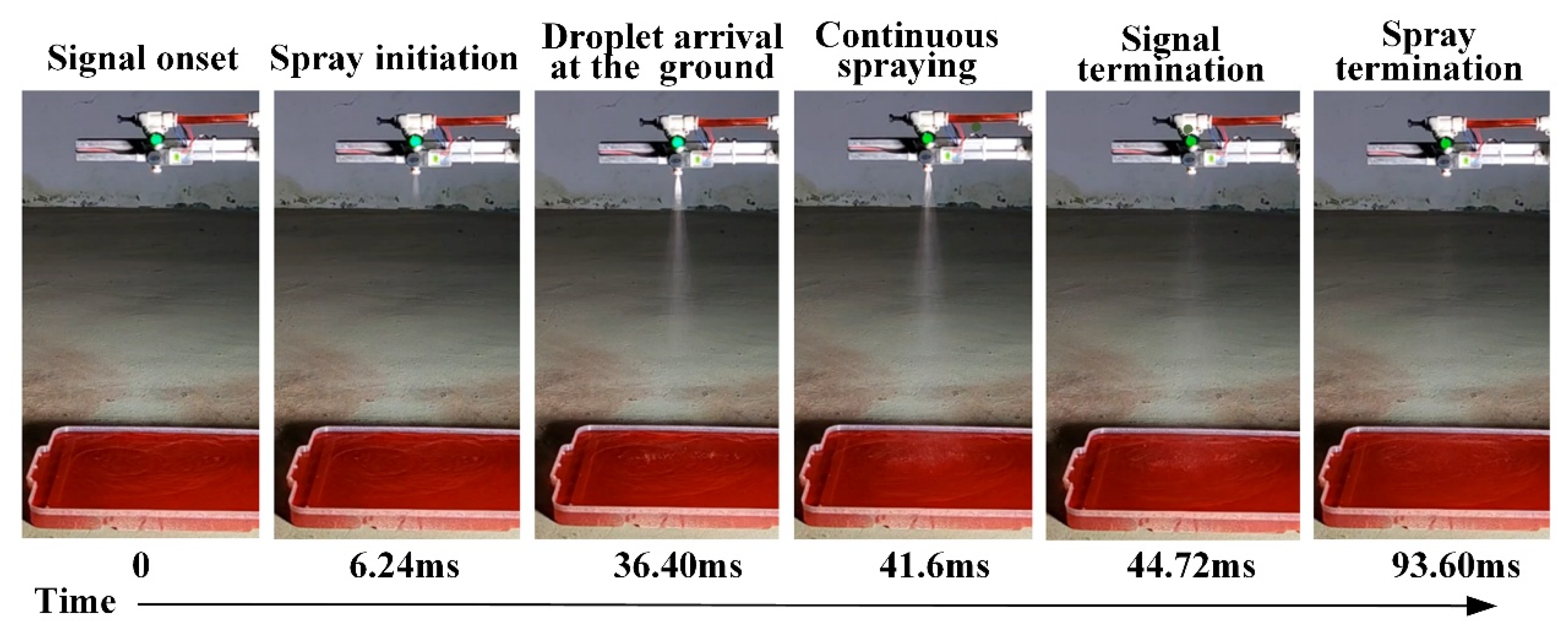
Figure 11.
Schematic illustration of the delay compensation method: (a) main view; (b) relative positions of the grid centerline and the spray centerline in the camera field of view.
Figure 11.
Schematic illustration of the delay compensation method: (a) main view; (b) relative positions of the grid centerline and the spray centerline in the camera field of view.
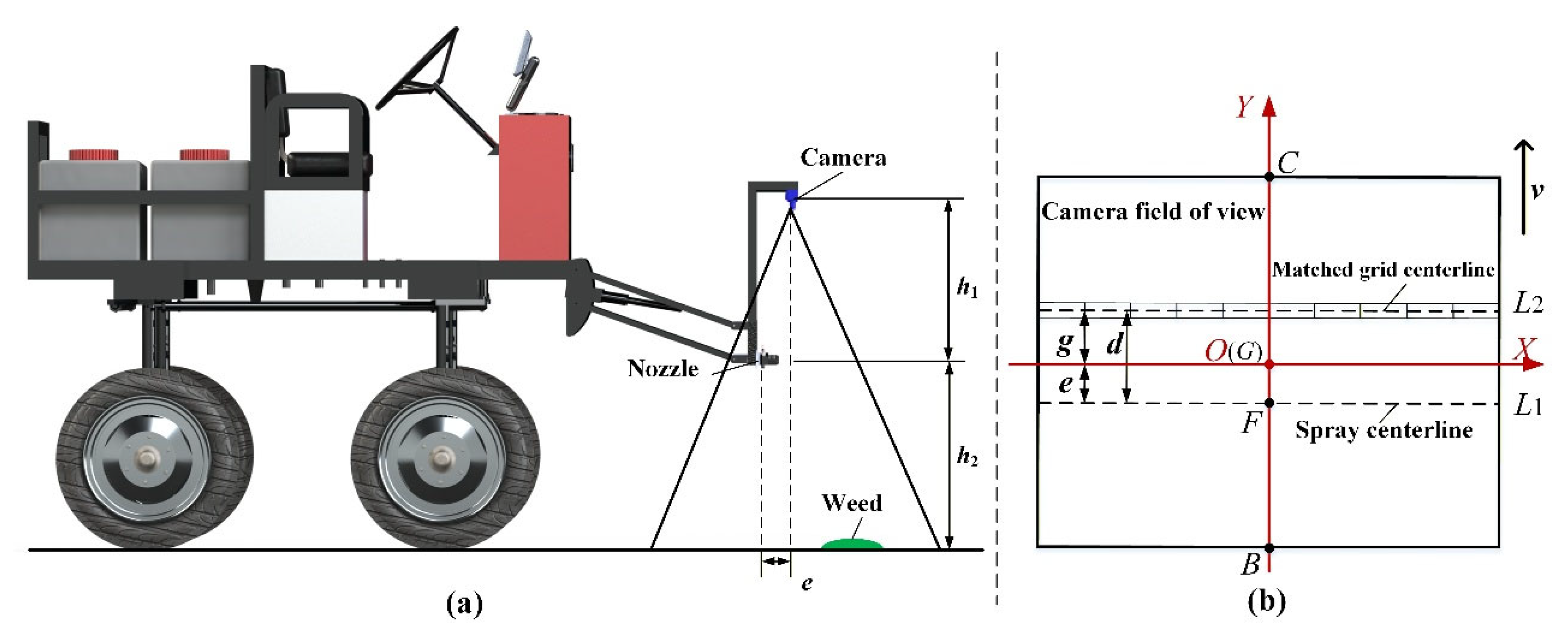
Figure 12.
Schematic diagram of the transformation between the world coordinate system and the pixel coordinate system.
Figure 12.
Schematic diagram of the transformation between the world coordinate system and the pixel coordinate system.
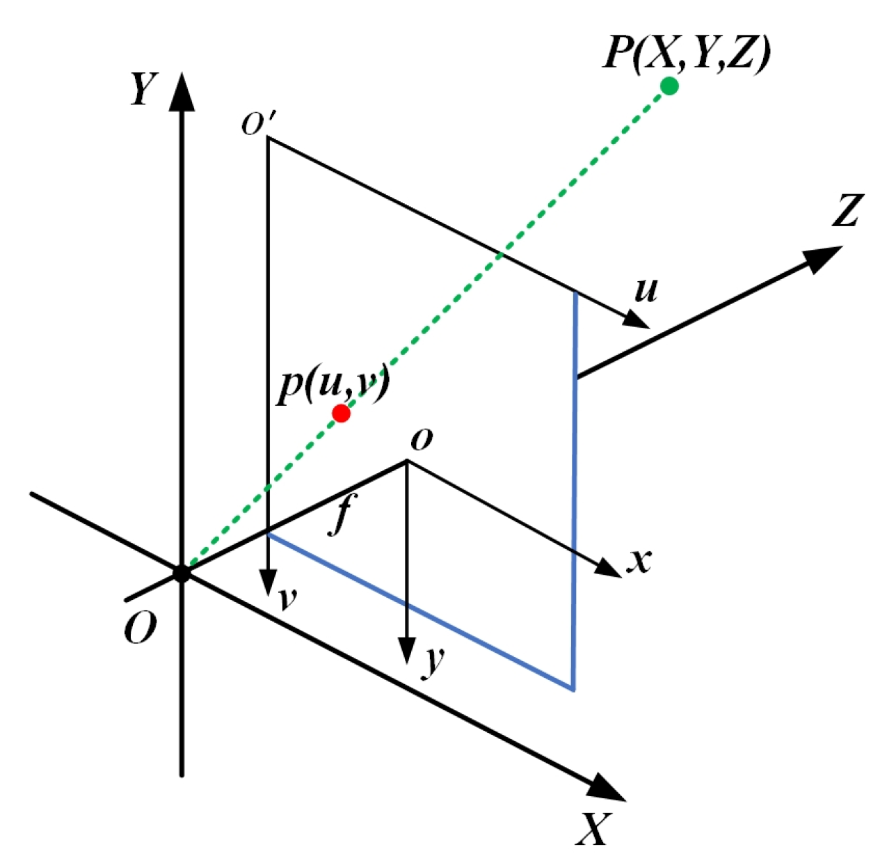
Figure 13.
Schematic diagram of overspray compensation: (a) Overspray occurring after the stop signal; (b) Compensation achieved by advancing the stop signal.
Figure 13.
Schematic diagram of overspray compensation: (a) Overspray occurring after the stop signal; (b) Compensation achieved by advancing the stop signal.
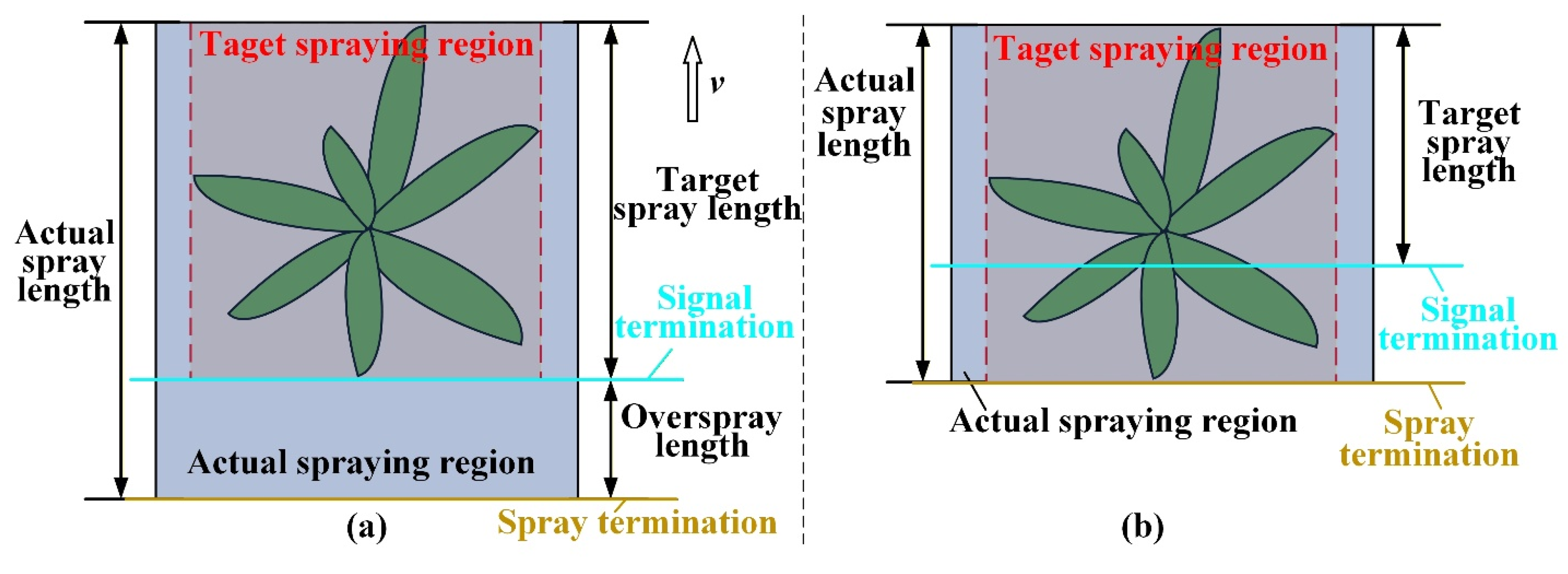
Figure 14.
Control flow chart the target spraying system
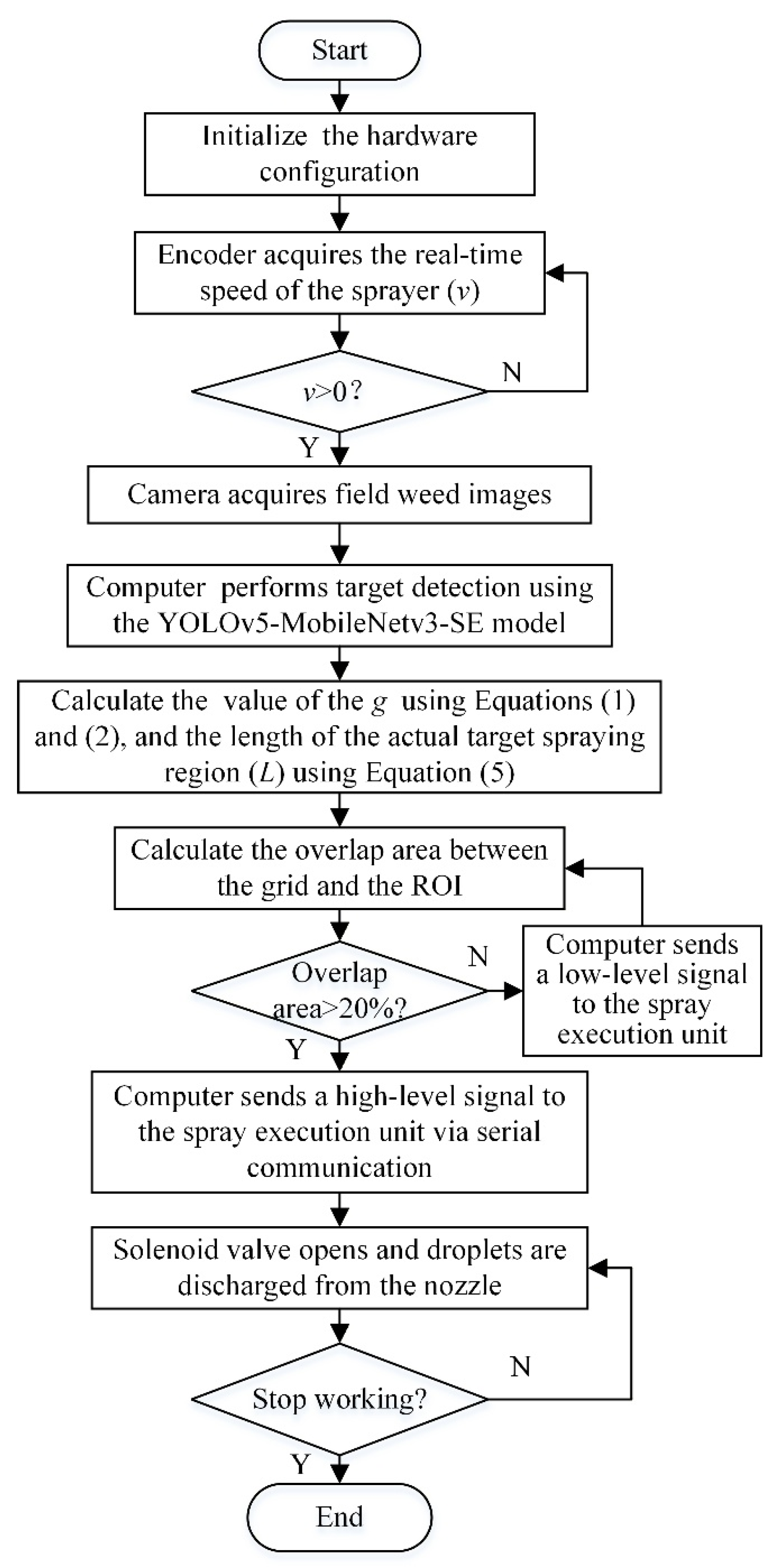
Figure 15.
Laboratory test platform for precision target spraying.
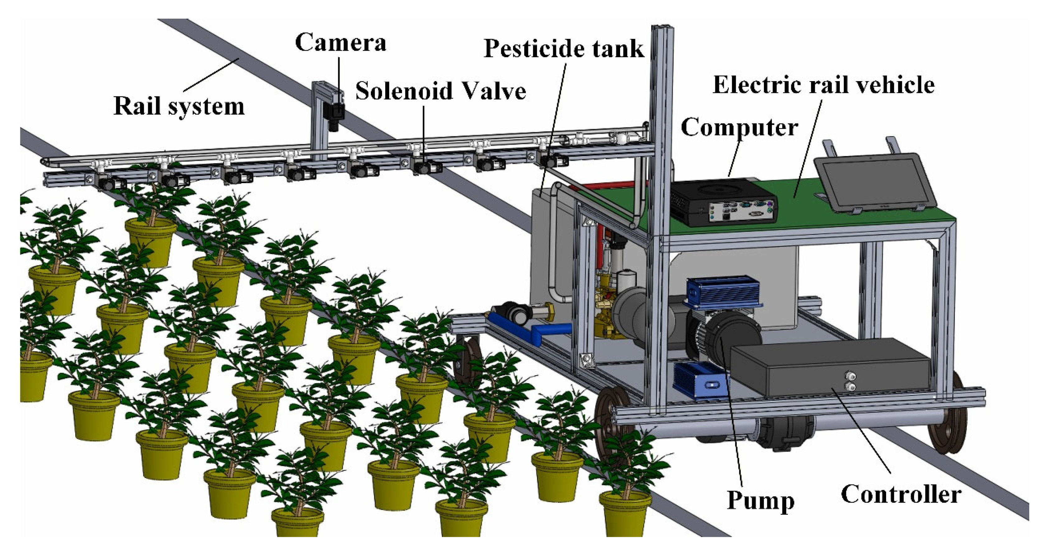
Figure 16.
Figure 16. Laboratory test setup for evaluating target spraying accuracy.
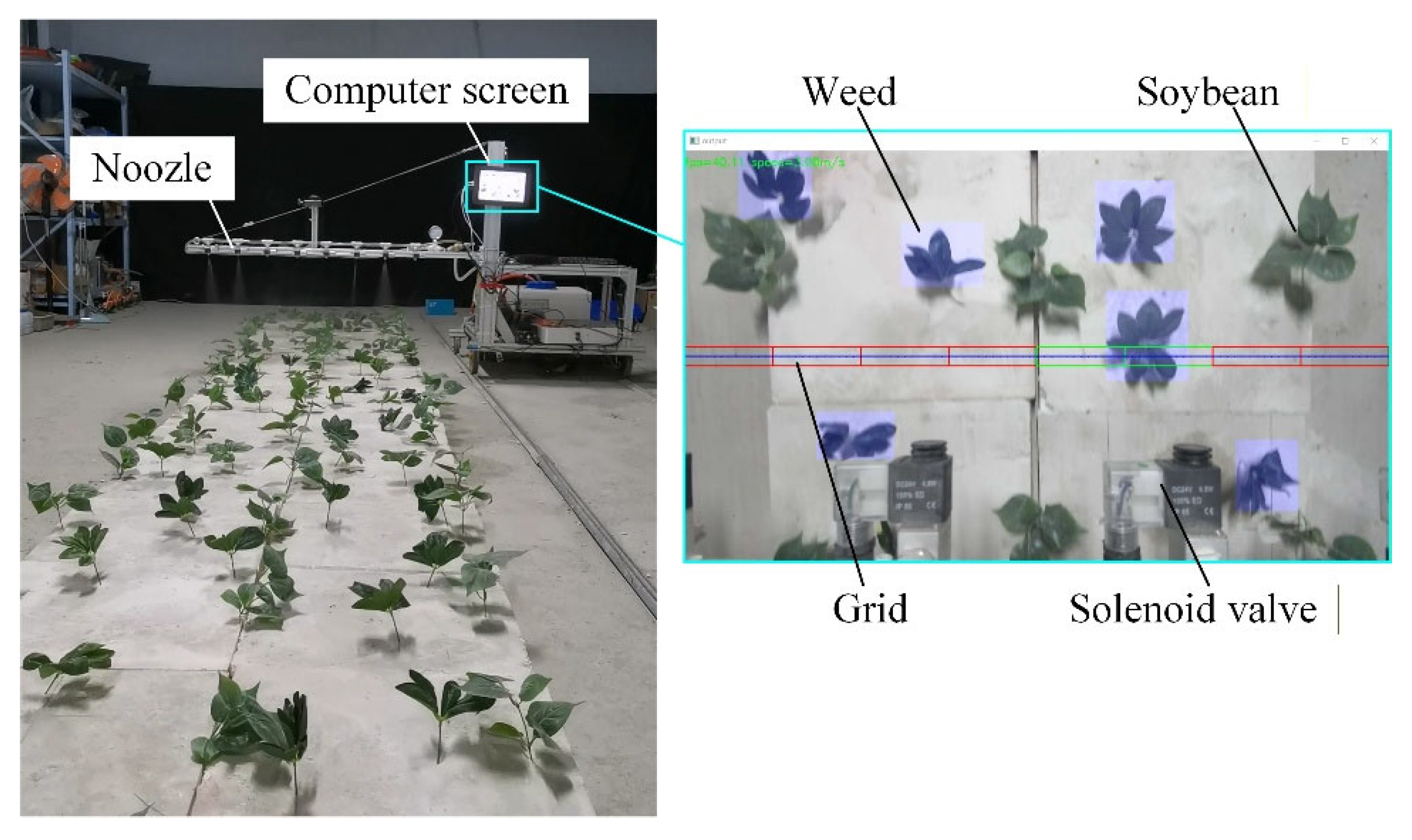
Figure 17.
Horizontal droplet distribution scanner used to measure spray distribution uniformity.
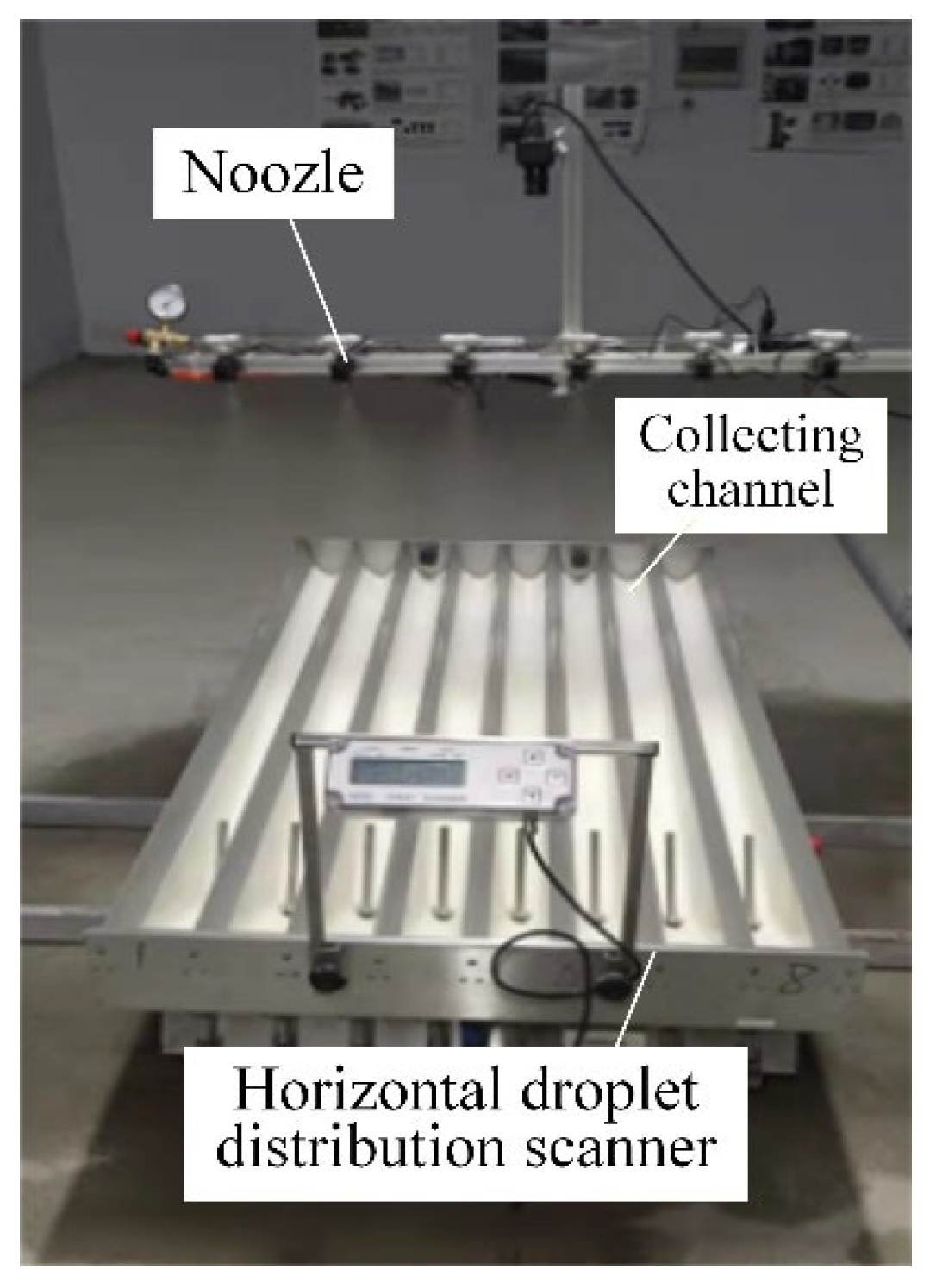
Figure 18.
Field experiment setup of the target spraying device prototype
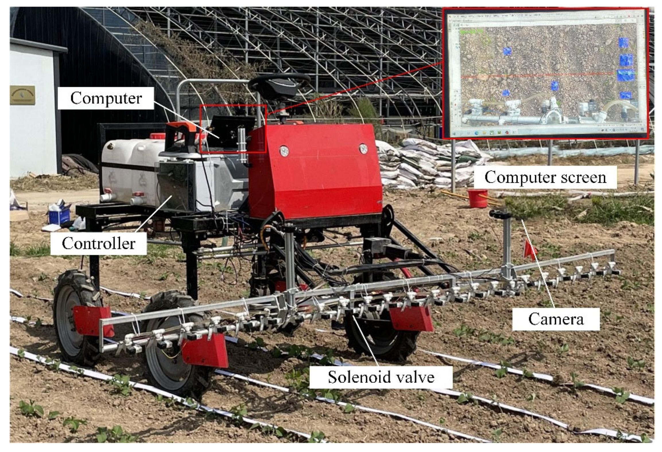
Figure 19.
Method for assessing spray coverage on weeds: (a) no droplet deposition; (b) droplet deposition indicating successful spraying.
Figure 19.
Method for assessing spray coverage on weeds: (a) no droplet deposition; (b) droplet deposition indicating successful spraying.
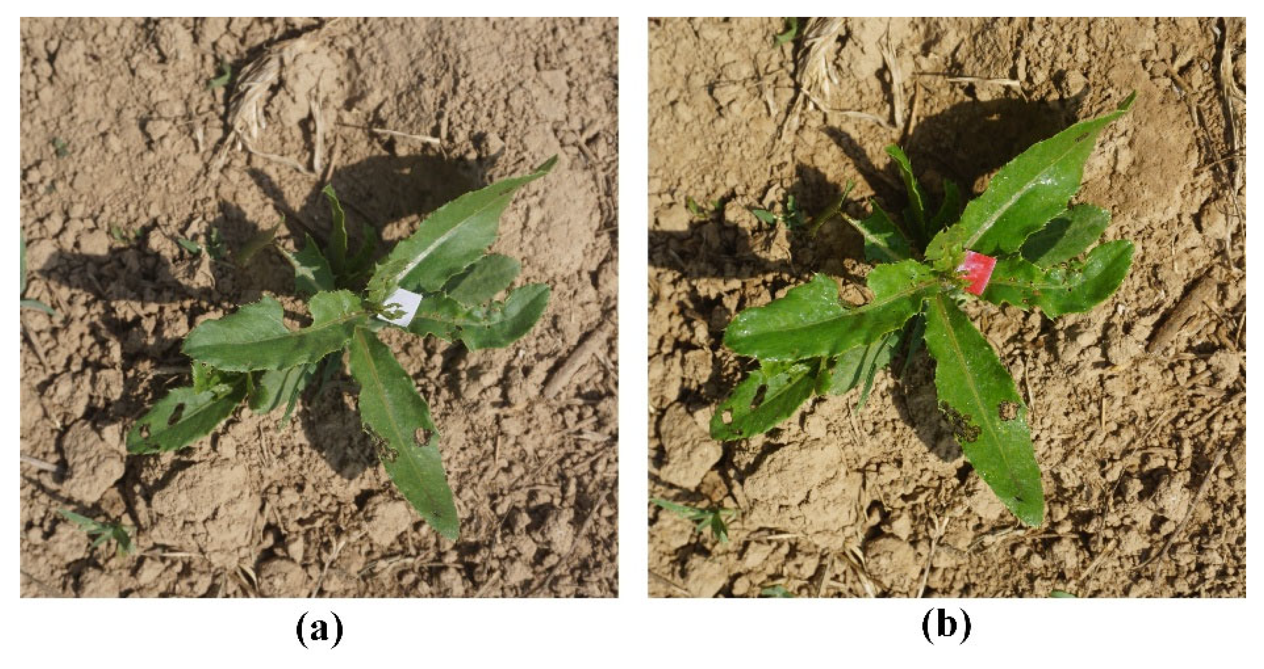

Table 1.
Technical parameters of the self-propelled boom sprayer.
| Parameter | Value |
| Overall dimensions (mm) | 2000×3000×1500 |
| Maximum operating speed (km·h⁻1) | 8 |
| Total weight (kg) | 450 |
| Pesticide tank capacity (L) | 200 |
| Spray boom width (mm) | 3000 |
| Ground clearance (mm) | 800 |
| Drive motor power (W) | 1600 |
| Battery pack voltage (V) | 60 |
Table 2.
Comparison of different models.
| Model | mAP0.5/% | Model size/MB | FPS |
|---|---|---|---|
| Faster R-CNN | 80.9 | 110.7 | 2.61 |
| YOLOv3 | 87.8 | 120.6 | 26.04 |
| YOLOv5s | 87.6 | 14.0 | 29.85 |
| YOLOv5x | 88.2 | 169.0 | 22.67 |
| YOLOv5_MobileNet-SE | 86.9 | 7.5 | 38.17 |
Table 3.
Target spraying accuracy test results at forward speeds of 1,2,3 and 4 km/h.
| Forward speed (km·h⁻1) |
Total number of weeds | Number of detected weeds | Number of weeds effectively sprayed | weed detection accuracy rate (%) | spraying accuracy rate (%) |
|---|---|---|---|---|---|
| 1 | 85 | 84 | 83 | 98.88 | 97.64 |
| 2 | 85 | 83 | 81 | 97.64 | 95.29 |
| 3 | 85 | 80 | 77 | 94.11 | 90.58 |
| 4 | 85 | 79 | 73 | 92.94 | 85.88 |
Table 4.
Pesticide reduction rates of precision target spraying under different weed coverage levels.
Table 4.
Pesticide reduction rates of precision target spraying under different weed coverage levels.
| Weed coverage rate (%) | Pesticide application rate of conventional continuous spraying (L) | Pesticide application rate of Precision target spraying (L) | Pesticide reduction rate (%) |
|---|---|---|---|
| 5 | 13.8 | 2.9 | 79.0 |
| 10 | 13.8 | 3.8 | 72.5 |
| 15 | 13.8 | 6.1 | 55.8 |
| 20 | 13.8 | 7.1 | 48.6 |
Table 5.
Field test results of the precision target spraying system at forward speeds of 2, 3, and 4 km·h⁻1.
Table 5.
Field test results of the precision target spraying system at forward speeds of 2, 3, and 4 km·h⁻1.
| Forward speed (km·h⁻1) |
Total number of weeds | Number of detected weeds | Number of weeds effectively sprayed | Weed detection accuracy rate (%) | Spraying accuracy rate (%) |
|---|---|---|---|---|---|
| 2 | 87 | 83 | 79 | 95.40 | 90.80 |
| 3 | 145 | 134 | 125 | 92.41 | 86.20 |
| 4 | 103 | 89 | 82 | 86.40 | 79.61 |
Disclaimer/Publisher’s Note: The statements, opinions and data contained in all publications are solely those of the individual author(s) and contributor(s) and not of MDPI and/or the editor(s). MDPI and/or the editor(s) disclaim responsibility for any injury to people or property resulting from any ideas, methods, instructions or products referred to in the content. |
© 2026 by the authors. Licensee MDPI, Basel, Switzerland. This article is an open access article distributed under the terms and conditions of the Creative Commons Attribution (CC BY) license (http://creativecommons.org/licenses/by/4.0/).
Copyright: This open access article is published under a Creative Commons CC BY 4.0 license, which permit the free download, distribution, and reuse, provided that the author and preprint are cited in any reuse.


