Submitted:
25 December 2025
Posted:
25 December 2025
You are already at the latest version
Abstract
To address the challenge of poor separation performance exhibited by conventional magnetic separation equipment when processing coarse-grained, low-grade magnetite ore, this paper proposes a novel ore recognition method that integrates empirical mode decomposition (EMD) with a convolutional neural network (CNN). First, the normalized magnetic induction intensity signals are decomposed using EMD to yield a series of intrinsic mode functions (IMFs). IMFs containing prominent characteristic information are then selected and fused based on their dominant frequency and kurtosis values, resulting in a reconstructed signal with significantly reduced noise. Subsequently, the reconstructed signals undergo inversion, re-normalization, and dimensional transformation into a two-dimensional matrix format to construct the training and testing sample datasets. A convolutional neural network is then designed and optimized to automatically extract discriminative features from these preprocessed samples, enabling accurate classification of magnetite ore grades. Experimental results demonstrate that the proposed EMD-CNN framework achieves effective and stable classification performance across different ore grades. In particular, the application of EMD for noise component removal substantially enhances the CNN’s recognition accuracy for waste rock and medium-grade ore, which are traditionally the most difficult categories to distinguish.
Keywords:
magnetite ore
; mineral separation
; sensor-based sorting
; convolutional neural network
; empirical mode decomposition
1. Introduction
Iron ore is one of the most essential raw materials in modern industrial systems, playing a crucial role in construction, manufacturing, energy, and numerous other sectors. With the sustained growth in global steel demand, high-grade iron ore resources have become increasingly depleted, making them insufficient to meet market requirements. Consequently, the exploitation and utilization of low-grade iron ore have escalated dramatically. However, low-grade iron ore must undergo beneficiation to increase its iron content to a level suitable for blast furnace or direct reduction processes. This typically involves multi-stage grinding and separation operations. Existing studies have shown that grinding accounts for the largest proportion of energy consumption and operational costs in the entire beneficiation process [1]. Therefore, implementing pre-concentration to discard waste rock at an early stage significantly reduces the volume of material entering subsequent grinding circuits, thereby lowering energy consumption and processing costs [2].
Since the early 21st century, ore pre-concentration technology has advanced from manual hand-sorting to sophisticated sensor-based sorting (SBS). Sensor-based sorting encompasses a range of automated techniques that detect individual particles using sensor-acquired data and subsequently separate them through mechanical, hydraulic, or pneumatic actuation. SBS has been widely adopted across various industries, including food and agricultural product processing, waste recycling, and mining. In agriculture, SBS is used to identify defects, shriveled or broken kernels, and pathogens in crops such as maize, rice, and wheat [3,4,5]. In recycling, it facilitates the classification of glass by color purity [6,7], the recovery of metals based on conductivity or magnetic permeability [8,9], and the sorting of construction and demolition waste through multi-sensor fusion [10,11,12,13,14,15]. In mining, SBS leverages differences in physical and chemical properties (e.g., color, reflectivity, conductivity, magnetic susceptibility, or atomic density) to separate valuable minerals from gangue. Representative techniques include X-ray transmission and dual-energy X-ray transmission sorting [16,17], magnetic resonance, and prompt gamma neutron activation analysis for copper ore grade detection [18], visible-range machine vision for gold-silver ore classification [19], and visible-near-infrared to short-wave infrared hyperspectral imaging for tin and copper ores [20]. Further applications of SBS in mining are comprehensively reviewed in [21,22,23].
Magnetite ore, a typical example of disseminated mineralization, contains intergrown valuable minerals and gangue. X-ray transmission imaging (Figure 1) shows that variations in iron grade do not produce distinct radiographic contrasts, while surface characteristics such as geometry and color are similarly indistinguishable between ore and gangue. Consequently, conventional SBS technologies have not been widely adopted for iron ore pre-concentration in industrial applications. However, magnetite exhibits strong magnetic susceptibility, which has led to the predominant use of magnetic separation in the iron ore industry. Magnetic separation exploits differences in magnetic susceptibility under controlled magnetic field intensity and gradient to achieve mineral separation. Coarse-grained magnetite ore typically undergoes dry or wet low-intensity magnetic separation before fine grinding. Numerous studies have focused on improving magnetic separator design and performance [24,25,26,27,28]. Despite these advances, conventional magnetic separators show limited effectiveness when processing coarse-grained, low-grade magnetite feeds, especially those with weakly magnetic or complex intergrowth characteristics. Furthermore, the production of high-performance permanent magnets requires substantial quantities of rare-earth elements (e.g., neodymium–iron–boron), and the separation process itself is both water- and energy-intensive, which conflicts with the principles of green and sustainable beneficiation. Against this background, conventional SBS technology has emerged as a pivotal research direction in intelligent mineral processing [2,22], providing valuable inspiration for the present study. This paper proposes a novel SBS method specifically tailored for magnetite ore (with potential applicability to other magnetic minerals). The underlying principle aligns with established SBS paradigms (e.g., X-ray transmission- or vision-based systems): a sensor acquires characteristic signals from individual particles, a deep learning model performs grade prediction and classification, and high-pressure air jets execute physical separation.
Convolutional neural networks (CNNs), first proposed by LeCun et al. in 1998, represent one of the most influential deep learning architectures and have achieved remarkable success in computer vision, speech recognition, and natural language processing [30]. Due to their exceptional capability for hierarchical feature extraction and high classification efficiency, CNNs have been increasingly adopted in SBS systems to enable rapid and accurate material recognition. In recent years, several studies have explored CNN-based approaches for mineral and rock classification, predominantly using two-dimensional inputs such as optical images, X-ray radiographs, or spectral data. Liu et al. [31] combined CNNs with transfer learning to classify 12 rock and mineral types, achieving an overall accuracy exceeding 70%, although the accuracy for magnetite remained below 60%. Pu et al. [32] applied a similar transfer-learning CNN framework to coal/gangue separation, attaining 82.5% accuracy. Zhou et al. [33] developed a CNN integrated with Squeeze-and-Excitation (SE) blocks to identify seven ore types, reaching 96% classification accuracy. More recently, Qiu et al. [34] employed CNN and Transformer models for photofluorescent uranium ore recognition, both surpassing 90% accuracy. Chen et al. [35] fused CNN with long short-term memory networks to extract spectral features of iron ore, achieving 91.67% recognition accuracy, while Yu et al. [36] utilized an improved YOLO architecture on UV-induced fluorescence images of spodumene, obtaining 90.2% accuracy. Despite these advances, existing CNN-based ore sorting methods have focused almost exclusively on two-dimensional visual or spectral data, whereas the classification of one-dimensional sensor signals–particularly magnetic induction signals–has received little attention.
To bridge this gap, this study proposes a CNN-based classification framework that directly processes one-dimensional magnetic induction signals acquired via Hall sensors mounted on a laboratory-scale magnetite separation device. To enhance signal quality and improve classification robustness, empirical mode decomposition (EMD) is employed for adaptive denoising before CNN input. The denoised signals are then reconstructed, transformed into two-dimensional representations, and fed into an optimized CNN for multi-class grade prediction. Finally, the reliability of the proposed classification method is validated through chemical assays of the sorted products. Although currently at the laboratory proof-of-concept stage and lacking evaluation of industrial-scale throughput or rejection rates, this work demonstrates the feasibility of intelligent magnetic-based sorting and offers a promising new paradigm for the pre-concentration of magnetite and other magnetic minerals. The subsequent sections are organized as follows: Section 2 establishes a magnetite ore sorting system bansed on Hall sensors, Section 3 introduces the acquisition and processing of the magnetic field signal, Section 4 disscusses the issue of magnetite ore identification, Section 5 conducts magnetite ore recognition experimentcarries, and finally Section 6 concludes this paper.
2. Magnetite Ore Sorting System Based on Hall Sensors
2.1. Magnetite Ore Sorting Principle
Any mineral exhibits a certain degree of magnetism when subjected to an external magnetic field, a phenomenon known as magnetization. Based on magnetic susceptibility, ores can be classified as either strongly magnetic or weakly magnetic, with magnetite belonging to the former category. Previous studies have shown that, under specific conditions, the magnetization of magnetite increases with increasing external magnetic field strength, and this relationship can be described by the following equation [37].
where is the total magnetic field intensity, is the external magnetic field intensity, is the magnetization intensity of ore, is the relative permeability, and is the specific magnetic coefficient.
When magnetite is placed in an external magnetic field, the total magnetic field intensity consists of the applied external field and the magnetic field induced within the ore. If the external magnetic field remains constant, variations in the total magnetic field intensity are solely determined by changes in the ore’s magnetic intensity. For a given ore particle entering the magnetic field, the induced magnetic intensity is fixed, resulting in a corresponding fixed variation in the total magnetic field intensity. Therefore, any change in this variation indicates the presence of additional ore particles within the magnetic field. Moreover, greater variations in the total magnetic field intensity correspond to stronger magnetism and, consequently, higher ore grades. Therefore, magnetic sensors can be used to detect these variations, providing a quantitative basis for evaluating ore grade and enabling effective sorting of ore and gangue.
A Hall sensor is a magnetic field sensor that operates based on the Hall effect and is capable of measuring variations in magnetic field intensity. As previously discussed, when a Hall sensor is exposed exclusively to an external magnetic field, the detected magnetic field intensity remains constant, provided the external field does not change. Minor fluctuations in the sensor output may occur due to factors such as signal transmission, thermal effects, and mechanical vibrations of electronic components; however, these fluctuations are considered negligible and are treated as a constant background. When magnetite passes through the sensing region, the magnetic field intensity detected by the Hall sensor changes relative to the background external magnetic field. Figure 2 illustrates the magnetic field variations produced by ores with different magnetic intensities under an external magnetic field. These variations correspond to the induced magnetic intensity of magnetite and serve as the fundamental feature for ore grade identification.
2.2. Magnetite Ore Sorting Device
Based on the principle of magnetite sorting, this study designs a Hall-sensor-based magnetite sorting device, as illustrated in Figure 3. The device comprises the following components: (1) a vibrating feeder, (2) a conveyor belt, (3) a permanent magnet assembly, (4) a Hall sensor detection unit, (5) a signal acquisition unit, (6) a signal processing and recognition unit, (7) a compressed air supply unit, (8) a separation unit, (9) a concentrate hopper, and (10) a tailings hopper.
The sorting process operates as follows. Ore particles are first dispersed and uniformly distributed onto the conveyor belt by the vibrating feeder. As the particles pass through the detection zone, the Hall sensor measures variations in the magnetic field and transmits the acquired signals to the signal processing and recognition unit via the signal acquisition unit. A pre-trained CNN model is then employed to predict and classify the magnetic field signals. The classification results are sent to a solenoid valve controller, which regulates the air nozzle based on the received commands to separate ores of different grades, directing them into either the concentrate hopper or the tailings hopper.
The main operating parameters of the sorting device are as follows: the Hall sensor sensitivity is 50 mV/Gs, the data acquisition card has a 16-bit resolution, the maximum sampling rate is 1000 Hz, the external magnetic field intensity in the sensor detection region is approximately 50 Gs, and the maximum conveyor belt speed is 3 m/s.
3. Signal Acquisition and Processing
As shown in Figure 2, the magnetic field signals detected by the Hall sensor fluctuate within a certain range due to external disturbances; these fluctuations are referred to as noise. It can be observed that the magnetic field intensity generated by low-grade ores is comparable in magnitude to the noise level, making it difficult to distinguish and thereby adversely affecting the accuracy of system judgment. Therefore, before CNN-based recognition of ore magnetic field signals, the acquired signals must be preprocessed to suppress noise and enhance discriminative features. The preprocessing procedure applied to the collected signals is illustrated in the Input Data Preprocessing module in Figure 4.
3.1. Signal Acquisition and Standardized Processing
The magnetic field signal of the ore is acquired using a Hall sensor to obtain the raw data, as shown in Figure 4(a). To highlight the dynamic variations in the magnetic induction signal, the raw data is standardized by removing its direct current (DC) component, as illustrated in Figure 4(b). The underlying calculation principle is described as follows:
where denotes the variation at the j-th sampling point of the i-th ore, represents the amplitude at the j-th sampling point of the i-th ore, and corresponds to the direct-current component of the signal associated with the i-th ore.
3.2. EMD Decomposition and Reconstruction
EMD is well-suited for processing non-stationary and nonlinear signals because it can adaptively decompose a signal into several intrinsic mode functions (IMFs) components and a residual component[38]. Each IMF must satisfy two specific conditions:
- Given the original signal , all local extrema are first identified. The upper envelope and lower envelope are then constructed using cubic spline interpolation of the local maxima and minima, respectively.
- The mean envelope is calculated from and , and the first component is obtained by subtracting from the original signal.
Based on the above conditions, the EMD procedure for the original signal can be summarized as follows:
: For the original signal , all local extrema are first identified, and the upper envelope and lower envelope are then constructed using cubic spline interpolation.
: Calculate the mean value M1 of the upper and lower envelopes, and determine the first component H1 by using the following equation
: Determine whether satisfies the two conditions required for an IMF component. If it does, is the first IMF component of ; otherwise, treat it as the new original signal and repeat Step 1 and step 2. Suppose the IMF component conditions are satisfied for the k-th time; then the first IMF component can be obtained according to the following equation
: Separate from to obtain the residual component .
: Treat as the new original signal and repeat step 1 through step 4 for n times to obtain the n-th IMF component .
The decomposition process terminates when becomes a monotonic function and can no longer be decomposed further.
Finally, the standard signal can be represented as
The standardized signal was decomposed using EMD to extract multiple IMFs at different frequency levels, as illustrated in Figure 4(c). These IMFs contain both the ore’s magnetic field signal and various noise components. Notably, the ore’s magnetic signal is weaker in the higher-frequency IMFs but becomes more distinct in the lower-frequency IMFs. The boundary between the high- and low-frequency bands was determined using detrended fluctuation analysis (DFA)[39].
If all high-frequency IMFs were discarded, the magnetic signal from the ore would be significantly attenuated. To address this, only the two IMFs within the high-frequency band with the lowest kurtosis values–a statistic that reflects the peakedness and tail weight of the signal distribution–were removed. The remaining IMFs were then combined to reconstruct the denoised signal, as shown in Figure 4(d).
The kurtosis K is calculated according to the following equation
where denotes the i-th sample point of an IMF component and is the mean value of an IMF component.
3.3. Establishment of Sample Set
To fully leverage the CNN’s ability to extract discriminative features from the ore’s magnetic field characteristics, the reconstructed signal undergoes inversion, normalization, and dimensionality transformation. The processed signal is then used as input to the CNN.
3.3.1. Inversion Processing
Magnetite ores can generate both positive and negative magnetic field signals when exposed to an external magnetic field. In this study, the CNN employs the rectified linear unit (ReLU) activation function, which inherently maps all negative input values to zero. As a result, during CNN training, negative signal components are suppressed, potentially causing information loss.
To prevent the elimination of negatively valued features and to enhance model robustness, an inversion operation is applied to the negative portion of the signal, as illustrated in Figure 4(e). The calculation principle of the inversion process is described as follows:
3.3.2. Normalization Processing
The amplitude range of the magnetic field signal varies among ore samples. To facilitate computation, standardize the signal range, and accelerate model convergence, the inverted magnetic induction signal is normalized, as shown in Figure 4(f). The normalization is performed according to the following equation
where denotes the normalized value at the j-th sampling point of the i-th ore sample. Here, and represent the maximum and minimum values of all sampling points across the entire dataset, respectively.
3.3.3. Dimensionality Transformation
The Hall sensor samples each ore to produce a one-dimensional signal of size . Since CNNs are particularly effective at processing two-dimensional image data, the signal is reshaped into a two-dimensional representation and subsequently converted into an image, as illustrated in Figure 4(g).
4. Magnetite Ore Identification
After completing the input data preprocessing, a CNN is employed to extract discriminative features and classify the ore signals, as illustrated in the Feature Extraction and Classification modules shown in Figure 4.
4.1. CNN Principle
The CNN is a deep learning model derived from artificial neural networks and can be considered a specialized form of a multilayer perceptron. Its core principle involves constructing multiple learnable filters to automatically extract representative features from input data. A typical CNN architecture consists of convolutional layers, pooling layers, and fully connected layers. By alternately applying convolution and pooling operations, discriminative features are extracted from magnetic induction signals, which are then classified and output by the fully connected layers.
4.1.1. Convolution Layer
The convolutional layer comprises multiple convolutional kernels, whose primary function is to extract features from the input matrix through local connectivity and weight-sharing mechanisms. The computational principle underlying the convolution operation is described as follows
where i and j denote the spatial indices of the output matrix, m and n represent the spatial indices of the input matrix, represents the output of the convolution operation, denotes the input matrix, and denotes the convolution kernel parameter matrix..
To enhance the nonlinearity of the network, an activation function is typically applied after the convolution operation. Consequently, the final output of the convolutional layer can be expressed as
where denotes the activation function, is the output of the convolution operation, represents the bias matrix, and is the final output of the convolutional layer.
4.1.2. Pooling Layer
A pooling layer is connected after each convolutional layer. The primary function of pooling is downsampling, which compresses the output features of the preceding layer while retaining the most salient information. In practice, max-pooling is commonly used to extract the maximum value within a local neighborhood of the input feature map. The pooling operation can be expressed as follows
where denotes the output of the pooling layer, is the pooling window size, and is the output matrix of the convolutional layer.
4.1.3. Full Connection Layer
Before the features extracted from the final convolutional or pooling layer are fed into the fully connected layer, they are first flattened to match the input format expected by the fully connected layer. Each neuron in the fully connected layer is connected to every element of the flattened feature vector, enabling the integration of local features to perform identification and classification of the input samples. This operation can be expressed as follows
where denotes the output of the fully connected layer, and represent the weight matrix and bias vector, respectively, and is the flattened feature vector.
The final fully connected layer functions as the classification layer and contains the same number of neurons as there are ore classes. For multi-class classification tasks, the Softmax function is commonly used to convert the output values into a probability distribution ranging from 0 to 1, with the sum of all probabilities equal to 1. This operation can be expressed as follows,
where is the output of the i-th node, and C is the total number of output nodes, corresponding to the number of categories.
4.1.4. Activation Function
Activation functions are applied after convolutional and fully connected layers to reduce structural risk and enhance the network’s nonlinear representation capabilities. Common activation functions include Sigmoid, Tanh, and ReLU. ReLU is widely used in CNNs due to its advantages in mitigating the vanishing gradient problem and accelerating network convergence. The ReLU function is defined as follows:
where indicates that if , then ; otherwise, .
4.2. CNN Structure Design and Training
Based on the LeNet-5 architecture [40], the CNN framework proposed in this study is illustrated in Figure 4(h). The input layer receives image signals of size 32 × 32 × 32. The feature extraction and classification components consist of three convolutional-pooling layers and two fully connected layers, respectively. Guided by empirical knowledge and the input size, the number of convolutional kernels is set to 32, 64, and 128 for the three convolutional layers, each with a kernel size of 3 × 3 and a stride of 1. Both max pooling and average pooling can be employed; however, since the magnetic field intensity of the ore is the primary recognition feature, max pooling is adopted. The pooling window is set to 2 × 2 with a stride of 1.
The fully connected layers perform recognition and classification of the extracted features. Before entering these layers, the feature maps obtained from the convolutional and pooling operations are flattened and processed using the Dropout technique [41] with a dropout rate of 0.5 to prevent overfitting. Based on the number of parameters after flattening, the first fully connected layer is configured with 64 neurons. The second fully connected layer is responsible for feature classification and outputs the ore categories. In this study, ores are classified into four categories: waste ore, low-grade ore, medium-grade ore, and high-grade ore. Therefore, the second fully connected layer contains four neurons and employs the SoftMax activation function. Representative sensor signals collected from ores of different grades are shown in Figure 4(i), (j), (k), and (l). Detailed parameters for each layer are summarized in Table 1.
5. Experiment and Analysis
All experiments were conducted on a computer running the Windows 11 platform, equipped with a 12th Gen Intel(R) Core(TM) i5-12500 processor (2.50 GHz) and 16.0 GB of RAM. The proposed model was trained and tested using Python 3.11 and Keras 3.5.0.
5.1. Input Data Preprocessing
The magnetite ore sorting system, constructed as shown in Figure 3, is depi cted in Figure 5. The data acquisition card was configured with a sampling rate of 1000 Hz, and the conveyor belt operated at a speed of 0.1 m/s. A total of 1000 ore samples, with particle sizes ranging from 10 to 50 mm and representing four randomly selected grades, were collected from a concentrator plant in Northwest China, as illustrated in Figure 6. The magnetic field signals of these ore samples were acquired using the sorting system to create the dataset. The dataset was then randomly divided into a training set and a test set in an 8 : 2 ratio. The sample distribution is summarized in Table 2.
Data preprocessing was conducted on the sample set, and the processed data were used as input for the CNN. In this study, one ore sample was randomly selected from each ore category—waste ore, low-grade ore, medium-grade ore, and high-grade ore—designated as WR, LR, MR, and HR, respectively. These four samples were processed according to the procedure outlined in Figure 4 (Input Data Preprocessing). The raw signals acquired by the Hall sensor from the processed samples are shown in Figure 7. Subsequently, the raw signals were standardized and decomposed using EMD to obtain the IMF component of various orders.
DFA is a method used to analyze long-range correlations in time series data. Its scaling exponent, , characterizes the autocorrelation properties of the series: when < 0.5, the series exhibits long-range anti-correlation; when = 0.5, the series is uncorrelated (i.e., it shows no long-range correlation), and when > 0.5, the series exhibits long-range positive correlation[42]. In this study, the physical interpretation of is not the primary focus; rather, it is employed to distinguish high-frequency IMFs from low-frequency IMFs. Specifically, IMF components with ⩽ 0.5 are classified as high-frequency, whereas those with > 0.5 are considered low-frequency. For the IMF components of WR, LR, MR, and HR, the DFA subinterval lengths u were set to [4, 8, 16, 32, 64, 128, 512]. The resulting scaling exponents for each IMF component are listed in Table 3.
As shown in Table 3, for the WR, LR, MR, and HR samples, IMF0 through IMF2 are classified as high-frequency components, while the remaining IMFs correspond to low-frequency components. Consequently, the kurtosis values of IMF0 through IMF2 are calculated, and the two IMFs with the lowest kurtosis values are removed. The kurtosis values for each IMF order are listed in Table 4. Under these conditions, IMF1 and IMF2 are discarded. The reconstructed signal is then obtained by combining IMF0 with the low-frequency components, as illustrated in Figure 8.
To optimize the sample structure and reduce the computational complexity of the CNN, the reconstructed signals undergo inversion, normalization, and image processing. The resulting representations are shown in Figure 9. The same preprocessing procedure is applied to the entire sample set using the method described above.
5.2. Feature Extraction
Based on empirical experience, satisfactory training performance can be achieved when the number of training epochs exceeds 100 and the learning rate is set below 0.2. Accordingly, the model is trained for 100 epochs using the error backpropagation algorithm based on gradient descent. To accelerate convergence, the Adam optimizer is employed, with the learning rate set to 0.001 for the first 75 epochs and reduced to 0.0001 for the remaining 25 epochs. The cross-entropy loss function is used as the training objective. The resulting loss and accuracy curves are presented in Figure 10. As the number of training epochs increases, both curves gradually converge, indicating that the model reaches a stable training state.
5.3. Result Analysis
To present the classification performance for each category in the test set, a confusion matrix is used to provide a detailed analysis of the recognition results. As shown in Figure 11, the CNN achieves recognition accuracies exceeding 85% for all four ore categories. Specifically, the recognition accuracies for waste ore, low-grade ore, medium-grade ore, and high-grade ore are 88%, 90%, 100%, and 94%, respectively. The relatively high recognition rates for medium-grade and high-grade magnetite can be attributed to their stronger magnetism and more pronounced magnetic field characteristics.
To illustrate the feature-learning capabilities of each convolution–pooling layer in the CNN model, the t-distributed stochastic neighbor embedding (t-SNE) nonlinear dimensionality reduction algorithm is employed to project the high-dimensional feature vectors output by each layer into a two-dimensional space for visualization [43], as shown in Figure 12. The input-layer visualization represents the distribution of the original samples. Due to the inherent redundancy of the magnetic induction signals, samples from adjacent categories are difficult to distinguish at this stage, as shown in Figure 12a.
Figure 12b–d show the feature distributions after the first through third convolution-pooling layers, respectively. As the network depth increases, most samples become progressively more dispersed and cluster according to their respective categories; however, a small number of samples remain intermixed between adjacent classes. After processing by the fully connected layers, samples from different categories are clearly separated, as illustrated in Figure 12e, demonstrating the effectiveness of the proposed CNN in extracting discriminative features.
5.4. Comparative Analysis
The CNN without the EMD method for noise reduction was constructed and the other operations were the same as the one in this paper. The same sample set was used for training and testing. The EMD-CNN is used to represent the model in this paper. The prediction results of the CNN and the EMD-CNN are shown in Table 5. It can be seen that the EMD-CNN has a good identification effect, especially in the identification of waste ore and medium-strength ore, and its accuracy rate is and higher than that of the CNN, respectively. Experimental results show that EMD can effectively improve the recognition accuracy of the CNN for low-grade ore.
5.5. Ore Grade Assay
The sorted ore samples were sent to Slon Magnetic Separator Co., Ltd. for grade determination. The testing procedure consists of two stages–sample preparation and assay–as illustrated in Figure 13. During sample preparation, the bulk ore is crushed and ground into a fine powder. The assay stage involves oxidation and reduction reactions of the ore powder using reagents such as a sulfuric–phosphoric mixed acid, hydrochloric acid (HCl), stannous chloride (SnO2), sodium tungstate (Na2WO4), and sodium diphenylamine sulfonate (C12H10NNaO3S). The treated solution is then titrated with potassium dichromate (K2Cr2O7). Finally, the ore grade is calculated based on the mass of the sample and the volume of K2Cr2O7 consumed during titration.
The grade calculation is expressed as follows
where denotes the ore grade, C is the titer, B is the volume of K2Cr2O7 consumed, and A is the mass of the sample.
Based on the completed assays, the measured grades of the four classified ore types—WR, LR, MR, and HR—are 23.66%, 28.24%, 38.25%, and 46.23%, respectively. A comparison with the target grade ranges listed in Table Figure 2 shows that only the WR ore slightly exceeds its predefined acceptable range, while the grades of the other three ore types fall within their respective target ranges.
6. Summary and Conclusions
The proposed magnetite ore sorting device, which is based on Hall sensor detection, is currently at the laboratory stage and has not yet been tested or deployed in industrial mineral processing environments. However, experimental findings demonstrate the feasibility of magnetite sorting using SBS technology. The present study corroborates the hypothesis that the magnetic characteristics of magnetite can be effectively detected by Hall sensors. Furthermore, it is demonstrated that magnetite ores of different grades exhibit distinguishable magnetic signatures. The exploitation of this property resulted in the installation of Hall sensors beneath a conveyor belt, with the purpose of capturing the magnetic field variations induced by passing magnetite particles. The acquired signals were subsequently processed by a trained CNN model for identification and classification. Ore-gangue separation was ultimately achieved using a pneumatic sorting mechanism. The findings suggest that higher-grade magnetite generates more pronounced magnetic responses, which in turn results in higher recognition accuracy by the CNN model.
The efficacy of the proposed method is contingent upon the sensitivity and spatial configuration of the sensors. Sensors with enhanced sensitivity are capable of detecting weaker magnetic signals associated with lower-grade ores, thereby expanding the range of ore grades that can be sorted. Furthermore, the configuration of the sensors has been demonstrated to exert a substantial influence on the accuracy of grade measurement. In this study, a single-column matrix array was employed, which limits the ability to capture multi-directional magnetic information. Subsequent research endeavours will involve the exploration of multi-column matrix array configurations, with the objective of facilitating multi-point and multi-angle detection. Furthermore, it has been demonstrated that the recognition algorithm itself is a key factor affecting sorting performance. A comparative analysis between CNN and EMD-CNN demonstrates that incorporating appropriate noise-reduction preprocessing prior to CNN-based recognition can significantly enhance classification accuracy. This research is applicable to magnetic ores in general, and it provides a novel approach for magnetic mineral sorting. Furthermore, it emphasises the potential for collaboration between sensor manufacturers and mining enterprises, thereby promoting the development of intelligent sorting technologies for magnetic ores.
Author Contributions
Conceptualization, Y.R. and Y.Y.; methodology, J.W. and C.P.; data collection, Y.R., Y.Y., F.Y., W.C. and J.W.; data analysis, J.W., C.P., F.Y., W.C. and J.W.; writing–original draft preparation, Y.R. and Y.Y.; writing–review and editing, J.W., C.P., F.Y., W.C. and J.W.; project administration, J.W. and C.P. All authors have read and agreed to the published version of the manuscript.
Funding
This work was supported in part by the National Natural Science Foundation of China under Grant Nos. 62473041 and 72161019, in part by the Science, Technology & Innovation Project of Xiongan New Area under Grant No. 2023XAGG0062, in part by the University Teacher Innovation Foundation of Gansu Province under Grant No. 2025B-462, in part by the Science and Technology Research Project of Jiangxi Provincial Department of Education under Grant No. GJJ2501005, in part by the Doctoral Scientific Research Foundation of Nanchang Hangkong University under Grant No. EA202404164, and in part by the Doctoral Scientific Research Foundation of Hubei University of Technology under Grant No. BSQD2022002.
Data Availability Statement
Data will be made available on request from the corresponding author.
Conflicts of Interest
The authors declare no conflicts of interest.
References
- Baawuah, E.; Kelsey, C.; Addai-Mensah, J.; Skinner, W. Economic and socio-environmental benefits of dry beneficiation of magnetite ores. Minerals 2020, 10, 955. [Google Scholar] [CrossRef]
- Klein, B.; Bamber, A. Mineral sorting. In Mineral Processing and Extractive Metallurgy Handbook; Dunne, R. C., Kawatra, S. K., Eds.; Society for Mining,Metallurgy & Exploration: Englewood, CO, USA, 2019; pp. 763–786. [Google Scholar]
- Delwiche, S. R.; Pearson, T. C.; Brabec, D. L. High-speed optical sorting of soft wheat for reduction of deoxynivalenol. Plant Disease 2005, 89, 1214–1219. [Google Scholar] [CrossRef]
- Carmack, W. J.; Clark, A. J.; Dong, Y.; Van Sanford, D. A. Mass selection for reduced deoxynivalenol concentration using an optical sorter in SRW wheat. Agronomy 2019, 9, 816. [Google Scholar] [CrossRef]
- Shiferaw, B.; Smale, M.; Braun, H. J.; Duveiller, E.; Reynolds, M.; Muricho, G. Crops that feed the world 10. Past successes and future challenges to the role played by wheat in global food security. Food Security 2013, 5, 291–317. [Google Scholar] [CrossRef]
- Dias, N.; Garrinhas, I.; Maximo, A.; Belo, N.; Roque, P.; Carvalho, M. T. Recovery of glass from the inert fraction refused by MBT plants in a pilot plant. Waste Management 2015, 46, 201–211. [Google Scholar] [CrossRef]
- Bonifazi, G.; Serranti, S. Imaging spectroscopy based strategies for ceramic glass contaminants removal in glass recycling. Waste Management 2006, 26, 627–639. [Google Scholar] [CrossRef]
- Mesina, M. B.; De Jong, T. P. R.; Dalmijn, W. L. Automatic sorting of scrap metals with a combined electromagnetic and dual energy X-ray transmission sensor. Int. J. Miner. Process. 2007, 82, 222–232. [Google Scholar] [CrossRef]
- Picón, A.; Ghita, O.; Bereciartua, A.; Echazarra, J.; Whelan, P. F.; Iriondo, P. M. Real-time hyperspectral processing for automatic nonferrous material sorting. J. Electron. Imaging 2012, 21, 013018–013018. [Google Scholar] [CrossRef]
- Bäcker, P.; Maier, G.; Gruna, R.; Längle, T.; Beyerer, J. Detecting tar contaminated samples in road-rubble using hyperspectral imaging and texture analysis. In Proc. Opt. Characterization Mater. Conf. 2023, 11–21. [Google Scholar]
- Paranhos, R. S.; Cazacliu, B. G.; Sampaio, C. H.; Petter, C. O.; Neto, R. O.; Huchet, F. A sorting method to value recycled concrete. J. Cleaner Prod. 2016, 112, 2249–2258. [Google Scholar] [CrossRef]
- Dittrich, S.; Thome, V.; Nühlen, J.; Gruna, R.; Dörmann, J. Baucycle-verwertungsstrategie für feinkörnigen bauschutt. Bauphysik 2018, 40, 379–388. [Google Scholar] [CrossRef]
- Hollstein, F.; Cacho, Í.; Arnaiz, S.; Wohllebe, M. Challenges in automatic sorting of construction and demolition waste by hyperspectral imaging. In Advanced Environmental, Chemical, and Biological Sensing Technologies XIII 2016, 9862, 73–82. [Google Scholar]
- Seifert, S.; Dittrich, S.; Bach, J. Recovery of raw materials from ceramic waste materials for the refractory industry. Processes 2021, 9, 228. [Google Scholar] [CrossRef]
- Vegas, I.; Broos, K.; Nielsen, P.; Lambertz, O.; Lisbona, A. Upgrading the quality of mixed recycled aggregates from construction and demolition waste by using near-infrared sorting technology. Constr. Build. Mater. 2015, 75, 121–128. [Google Scholar] [CrossRef]
- Amar, H.; Benzaazoua, M.; Elghali, A.; Taha, Y.; El Ghorfi, M.; Krause, A.; Hakkou, R. Mine waste rock reprocessing using sensor-based sorting (SBS): Novel approach toward circular economy in phosphate mining. Miner. Eng. 2023, 204, 108415. [Google Scholar] [CrossRef]
- Robben, C.; Condori, P.; Pinto, A.; Machaca, R.; Takala, A. X-ray-transmission based ore sorting at the San Rafael tin mine. Miner. Eng. 2019, 145, 105870. [Google Scholar] [CrossRef]
- Cetin, M. C.; Klein, B.; Futcher, W. A conceptual strategy for effective bulk ore sorting of copper porphyries: exploiting the synergy between two sensor technologies. Miner. Eng. 2023, 201, 108182. [Google Scholar] [CrossRef]
- Shatwell, D. G.; Murray, V.; Barton, A. Real-time ore sorting using color and texture analysis. Int. J. Min. Sci. Technol. 2023, 33, 659–674. [Google Scholar] [CrossRef]
- Tuşa, L.; Kern, M.; Khodadadzadeh, M.; Blannin, R.; Gloaguen, R.; Gutzmer, J. Evaluating the performance of hyperspectral short-wave infrared sensors for the pre-sorting of complex ores using machine learning methods. Miner. Eng. 2020, 146, 106150. [Google Scholar] [CrossRef]
- Santos, E. G. D.; Brum, I. A. S. D.; Ambrós, W. M. Techniques of pre-concentration by sensor-based sorting and froth flotation concentration applied to sulfide ores–a review. Minerals 2025, 15, 350. [Google Scholar] [CrossRef]
- Maier, G.; Gruna, R.; Längle, T.; Beyerer, J. A survey of the state of the art in sensor-based sorting technology and research. IEEE Access 2024, 12, 6473–6493. [Google Scholar] [CrossRef]
- Robben, C.; Wotruba, H. Sensor-based ore sorting technology in mining–past, present and future. Minerals 2019, 9, 523. [Google Scholar] [CrossRef]
- Chokin, K. S.; Yedilbayev, A. I.; Yedilbayev, B. A.; Yugay, V. D. Dry magnetic separation of magnetite ores. Periódico Tchê Química 2020, 17. [Google Scholar] [CrossRef]
- Zhang, H.; Chen, L.; Zeng, J.; Ding, L.; Liu, J. Processing of lean iron ores by dry high intensity magnetic separation. Sep. Sci. Technol. 2015, 50, 1689–1694. [Google Scholar] [CrossRef]
- Chokin, K.; Yedilbayev, A.; Yugai, V.; Medvedev, A. Beneficiation of magnetically separated iron-containing ore waste. Processes 2022, 10, 2212. [Google Scholar] [CrossRef]
- Luo, X.; He, K.; Zhang, Y.; He, P.; Zhang, Y. A review of intelligent ore sorting technology and equipment development. Int. J. Miner. Metall. Mater. 2022, 29, 1647–1655. [Google Scholar] [CrossRef]
- Chen, L.; Xiong, D. Mineral sorting. In Progress in Filtration and Separation; Tarleton, S., Ed.; Academic Press: Pittsburgh, PA, USA, 2015; pp. 287–324. [Google Scholar]
- Maier, G.; Gruna, R.; Längle, T.; Beyerer, J. A survey of the state of the art in sensor-based sorting technology and research. IEEE Access 2024, 12, 6473–6493. [Google Scholar] [CrossRef]
- Gu, J.; Wang, Z.; Kuen, J.; Ma, L.; Shahroudy, A.; Shuai, B.; Liu, T.; Wang, X.; Wang, G.; Cai, J.; Chen, T. Recent advances in convolutional neural networks. Pattern Recognit. 2018, 77, 354–377. [Google Scholar] [CrossRef]
- Liu, C.; Li, M.; Zhang, Y.; Han, S.; Zhu, Y. An enhanced rock mineral recognition method integrating a deep learning model and clustering algorithm. Minerals 2019, 9, 516. [Google Scholar] [CrossRef]
- Pu, Y.; Apel, D. B.; Szmigiel, A.; Chen, J. Image recognition of coal and coal gangue using a convolutional neural network and transfer learning. Energies 2019, 12, 1735. [Google Scholar] [CrossRef]
- Zhou, W.; Wang, H.; Wan, Z. Ore image classification based on improved CNN. Comput. Electr. Eng. 2022, 99, 107819. [Google Scholar] [CrossRef]
- Qiu, J.; Zhang, Y.; Fu, C.; Yang, Y.; Ye, Y.; Wang, R.; Tang, B. Study on photofluorescent uranium ore sorting based on deep learning. Miner. Eng. 2024, 206, 108523. [Google Scholar] [CrossRef]
- Chen, H.; Xia, M.; Zhang, Y.; Zhao, R.; Song, B.; Bai, Y. Iron ore information extraction based on CNN-LSTM composite deep learning model. IEEE Access 2025. [Google Scholar] [CrossRef]
- Yu, T.; Zhu, Y.; Liu, J.; Han, Y.; Li, Y. Enhanced pre-selection of spodumene via ultraviolet-induced fluorescence and improved YOLOv8 deep learning algorithm. Miner. Eng. 2025, 230, 109432. [Google Scholar] [CrossRef]
- William, H. H.; Buck, J. A. Engineering electromagnetics, 9rd ed.; Tsinghua University Press: Beijing, China, 2019; pp. 184–187. [Google Scholar]
- Huang, N. E.; Shen, Z.; Long, S. R.; Wu, M. C.; Shih, H. H.; Zheng, Q.; Liu, H. H. The empirical mode decomposition and the Hilbert spectrum for nonlinear and non-stationary time series analysis. Proceedings of the Royal Society of London. Series A: mathematical, physical and engineering sciences 1998, 454, 903–995. [Google Scholar] [CrossRef]
- Peng, C. K.; Buldyrev, S. V.; Havlin, S.; Simons, M.; Stanley, H. E.; Goldberger, A. L. Mosaic organization of DNA nucleotides. Phys. Rev. E 1994, 49, 1685. [Google Scholar] [CrossRef]
- LeCun, Y.; Bottou, L.; Bengio, Y.; Haffner, P. Gradient-based learning applied to document recognition. Proc. IEEE 2002, 86, 2278–2324. [Google Scholar] [CrossRef]
- Hinton, G. E.; Srivastava, N.; Krizhevsky, A.; Sutskever, I.; Salakhutdinov, R. R. Improving neural networks by preventing co-adaptation of feature detectors. arXiv 2012, arXiv:1207.0580. [Google Scholar] [CrossRef]
- Rodriguez, E.; Echeverria, J. C.; Alvarez-Ramirez, J. Detrended fluctuation analysis of heart intrabeat dynamics. Physica A 2007, 384, 429–438. [Google Scholar] [CrossRef]
- Maaten, L. V. D.; Hinton, G. Visualizing data using t-SNE. J. Mach. Learn. Res. 2008, 9, 2579–2605. [Google Scholar]
Figure 1.
Ore X-ray imaging. (a) Waste grade. (b) Low grade. (c) Medum grade. (d) High grade.
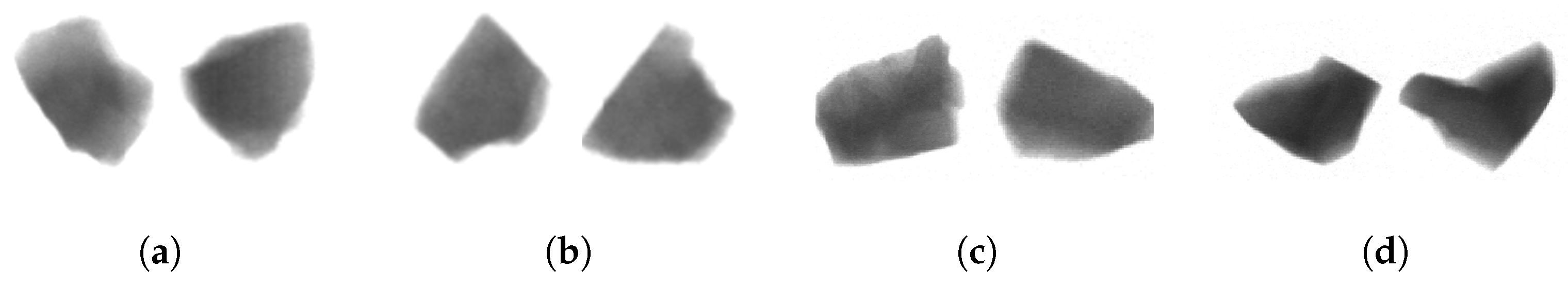
Figure 2.
Changes of magnetic field intensity.
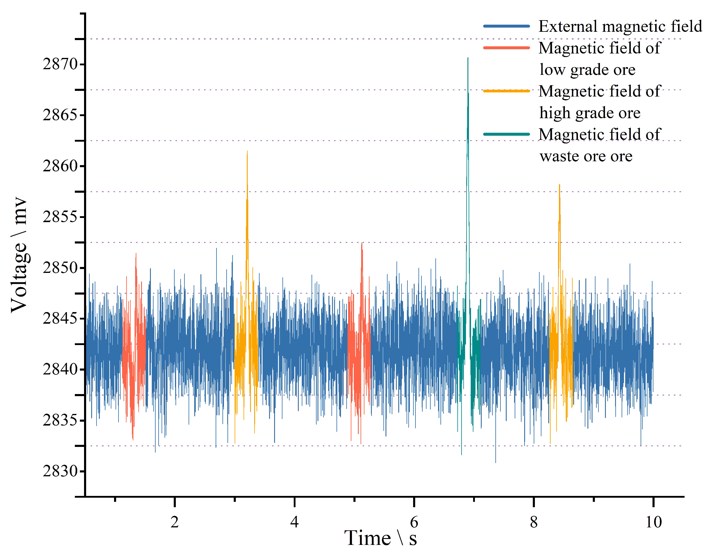
Figure 3.
Magnetite sorting device.
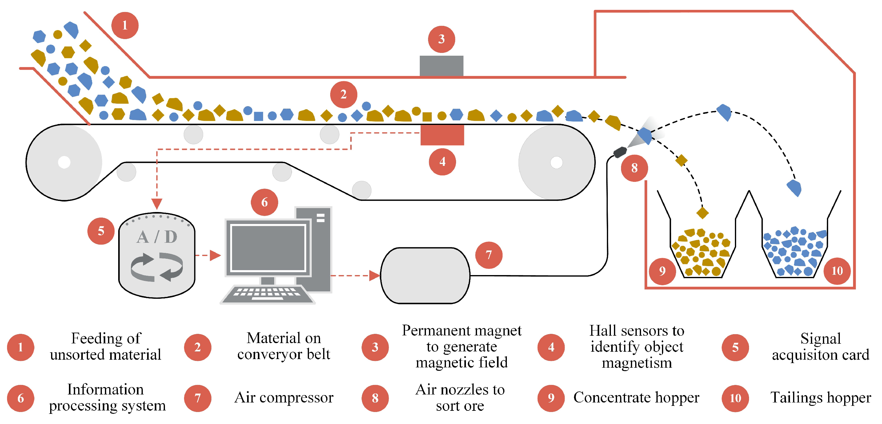
Figure 4.
Ore signals processing and recognition process.
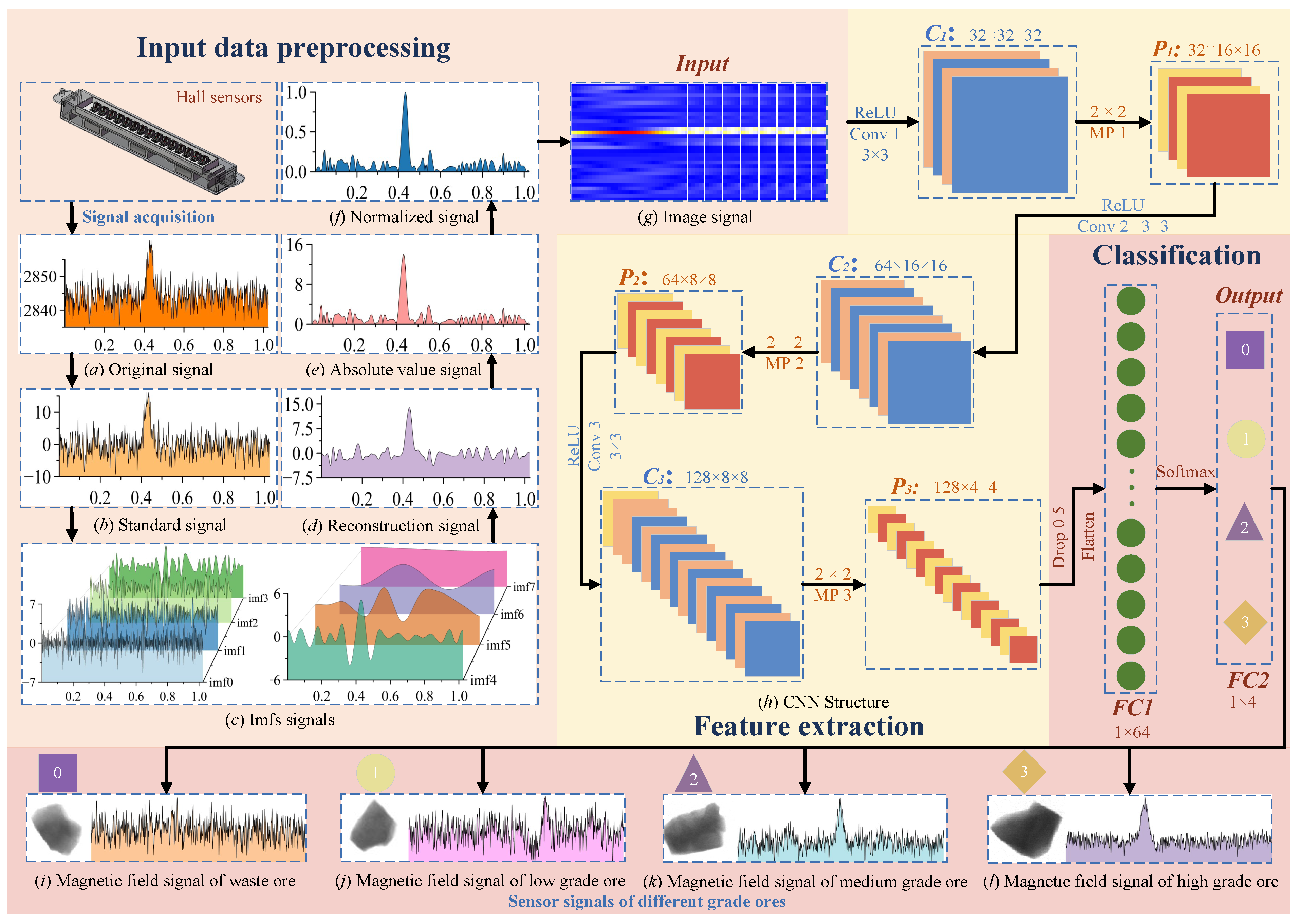
Figure 5.
Magnetite sorting system.
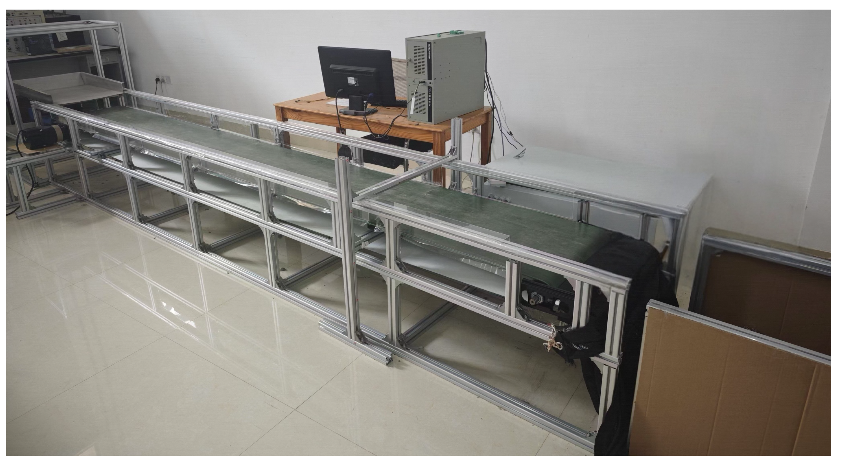
Figure 6.
Four grades of ore. (a) Waste grade. (b) Low grade. (c) Medum grade. (d) High grade.
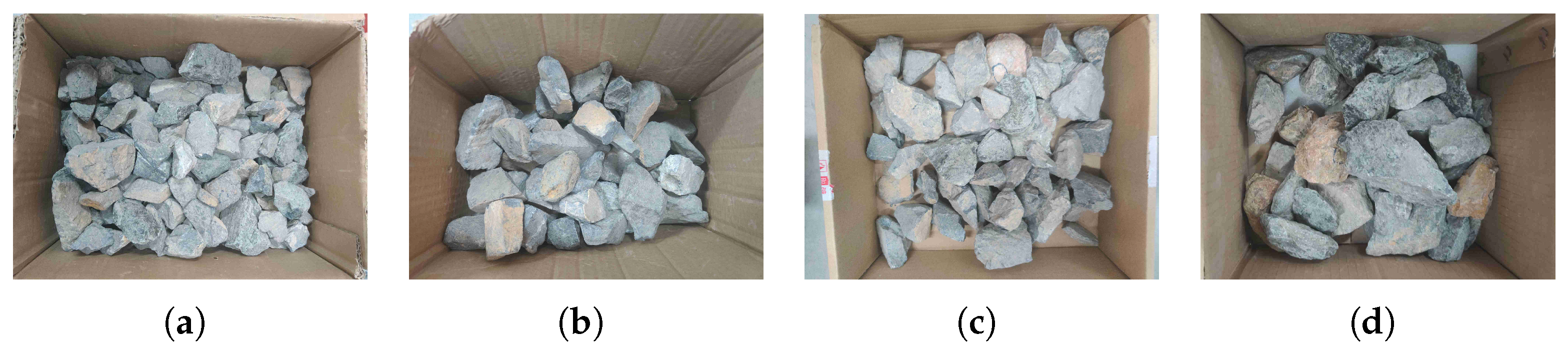
Figure 7.
Original signal of 4 ores.
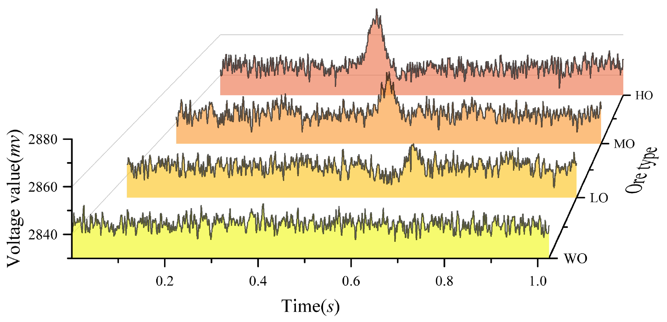
Figure 8.
Construction signal of 4 ores. (a) WR signals. (b) LR signals. (c) MR signals. (d) HR signals.
Figure 8.
Construction signal of 4 ores. (a) WR signals. (b) LR signals. (c) MR signals. (d) HR signals.
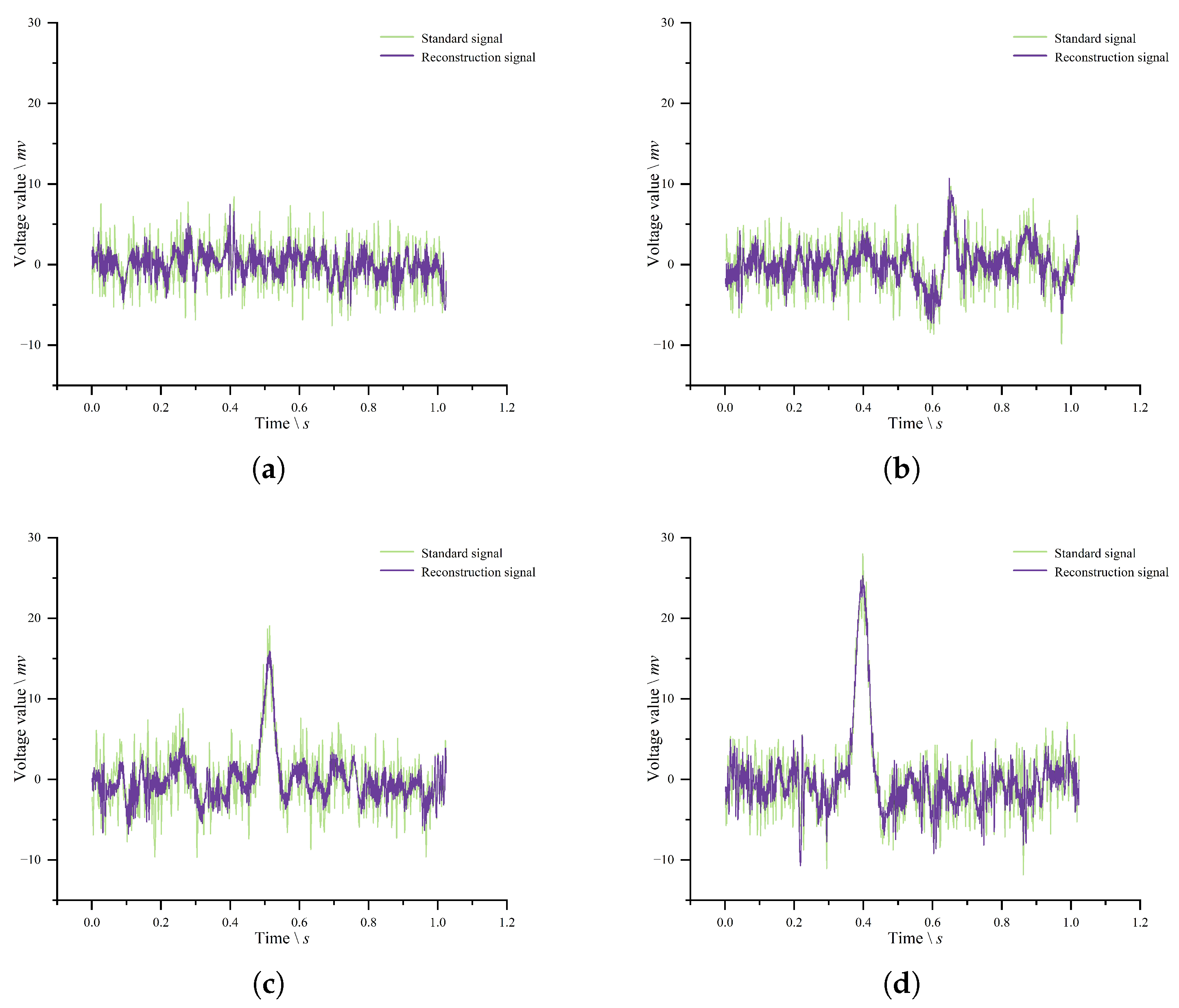
Figure 9.
Image signal of four ores. (a) Image signal of WR. (b) Image signal of LR. (c) Image signal of MR. (d) Image signal of HR.
Figure 9.
Image signal of four ores. (a) Image signal of WR. (b) Image signal of LR. (c) Image signal of MR. (d) Image signal of HR.
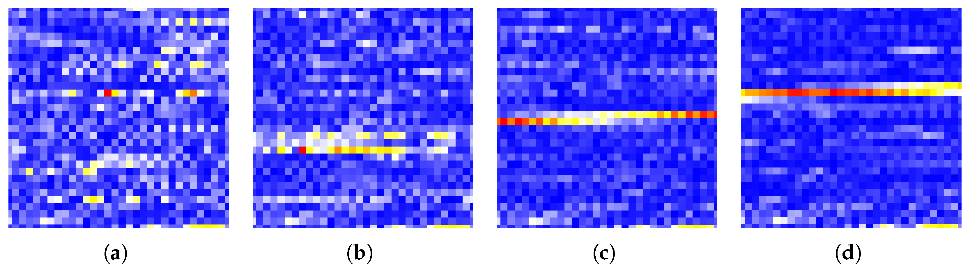
Figure 10.
Loss and accuracy curve.
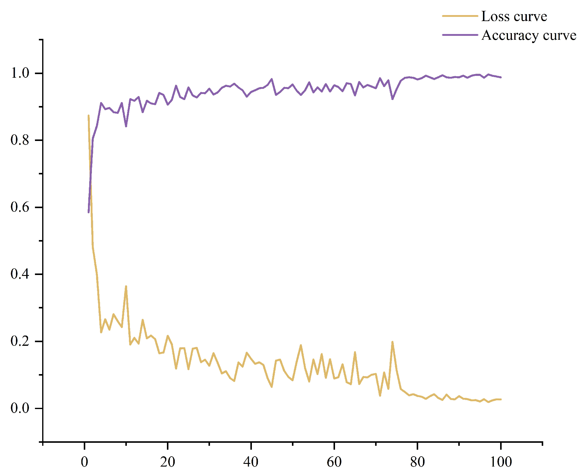
Figure 11.
Confusion matrix.
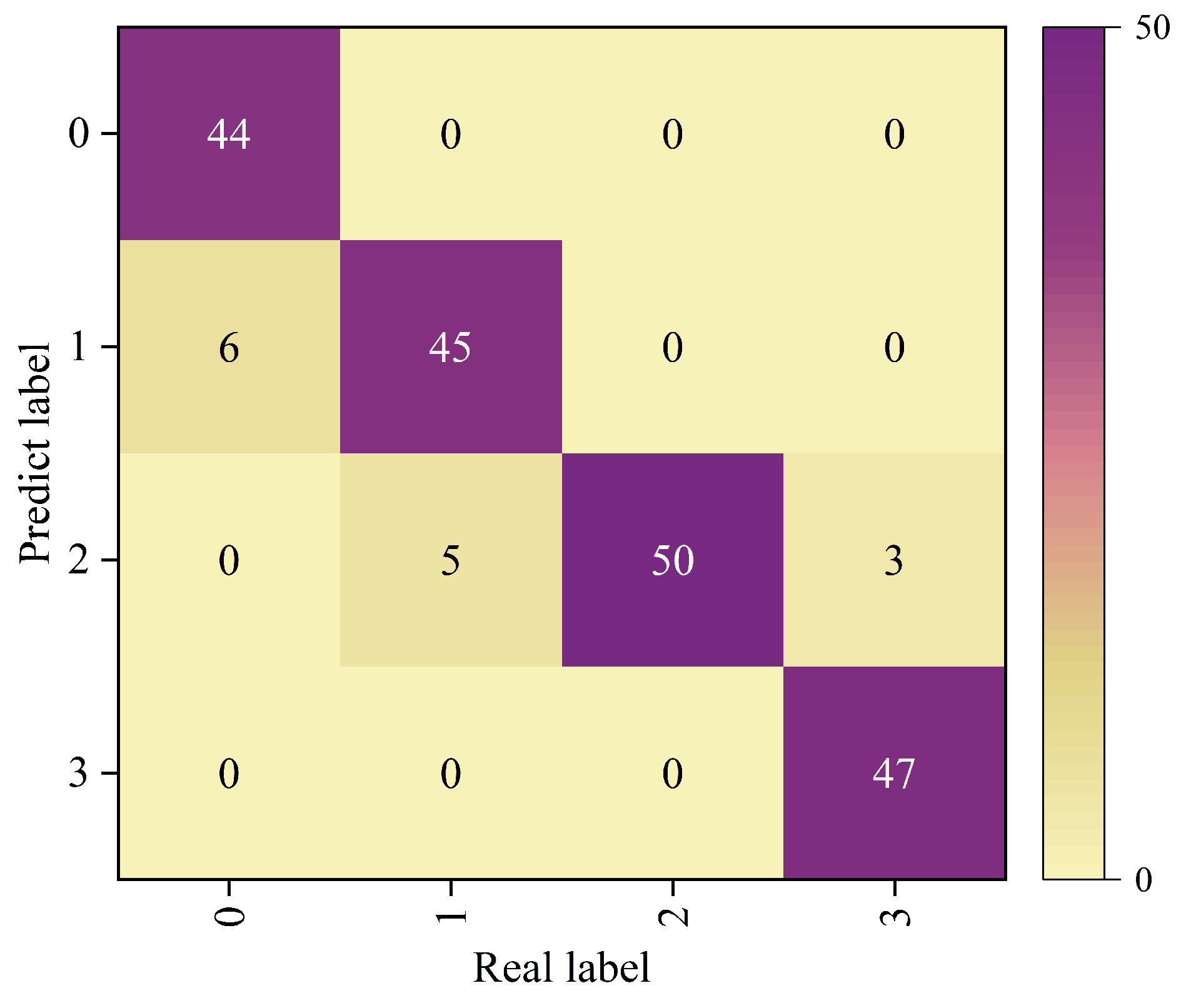
Figure 12.
Visual output. (a) Input. (b) First layer. (c) Second layer. (d) Third layer. (e) Output.
Figure 12.
Visual output. (a) Input. (b) First layer. (c) Second layer. (d) Third layer. (e) Output.
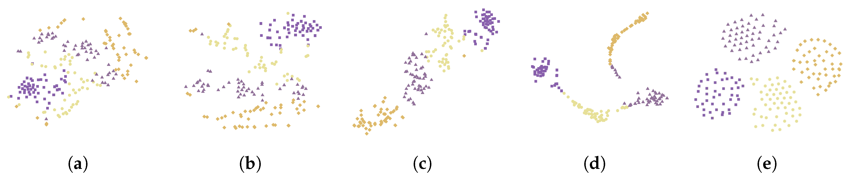
Figure 13.
Sample preparation and assay process.
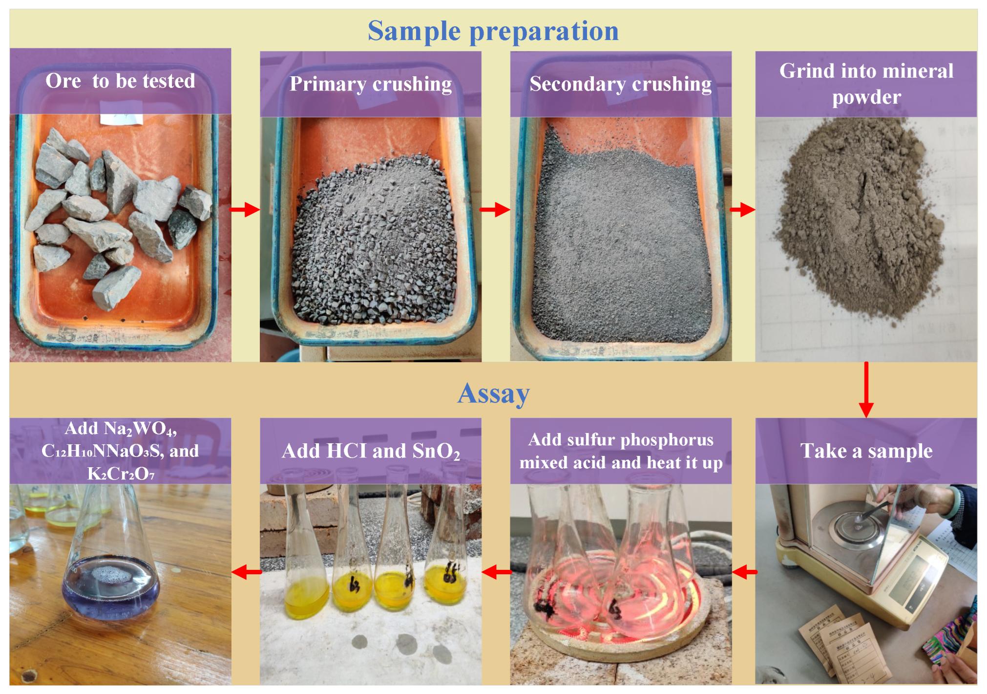

Table 1.
Parameters of each layer of CNN.
| Structure | Size | Number | Strides | Padding | Activity function |
|---|---|---|---|---|---|
| C 1 | 3×3 | 32 | 1 | Same | ReLU |
| P 1 | 2×2 | 32 | 1 | - | - |
| C 2 | 3×3 | 64 | 1 | Same | ReLU |
| P 2 | 2×2 | 64 | 1 | - | - |
| C 3 | 3×3 | 128 | 1 | Same | ReLU |
| P 3 | 2×2 | 128 | 1 | - | - |
| Flatten | - | - | - | - | - |
| Dropout | - | - | - | - | - |
| FC 1 | - | 64 | - | - | ReLU |
| FC 2 | - | 4 | - | - | SoftMax |
Table 2.
Sample distribution.
| Sample set | Grade | Label | Training set | Test set | Sum |
|---|---|---|---|---|---|
| Waste ore | 0 | 200 | 50 | 250 | |
| Low-grade ore | 1 | 200 | 50 | 250 | |
| Medium-grade ore | 2 | 200 | 50 | 250 | |
| High-grade ore | 3 | 200 | 50 | 250 | |
| Sum | - | - | 800 | 2000 | 1000 |
Table 3.
Scaling exponents of IMFs.
| Ore types | IMF0 | IMF1 | IMF2 | IMF3 | IMF4 | IMF5 | IMF6 | IMF7 |
|---|---|---|---|---|---|---|---|---|
| WR | 0.069 | 0.156 | 0.372 | 0.755 | 1.180 | 1.622 | 1.931 | - |
| LR | 0.053 | 0.183 | 0.424 | 0.742 | 1.249 | 1.629 | 1.858 | 2.036 |
| MR | 0.061 | 0.195 | 0.428 | 0.982 | 1.296 | 1.738 | 1.841 | - |
| HR | 0.098 | 0.214 | 0.479 | 0.905 | 1.458 | 1.669 | 1.892 | 2.013 |
Table 4.
Kurtosis of IMFs.
| Ore types | IMF0 | IMF1 | IMF2 | IMF3 | IMF4 | IMF5 | IMF6 | IMF7 |
|---|---|---|---|---|---|---|---|---|
| WR | 3.85 | 3.03 | 2.89 | 2.88 | 2.32 | 2.58 | 1.75 | - |
| LR | 3.29 | 3.17 | 3.15 | 4.81 | 5.47 | 3.08 | 1.70 | 1.38 |
| MR | 3.45 | 3.19 | 2.81 | 6.46 | 2.23 | 3.40 | 1.96 | - |
| HR | 5.61 | 3.18 | 3.17 | 7.49 | 7.62 | 3.53 | 1.71 | 1.72 |
Table 5.
Prediction result.
| Ore types | CNN prediction | EMD-CNN prediction |
|---|---|---|
| WR | 76.1% | 88% |
| LR | 90% | 90% |
| MR | 82.2% | 100% |
| HR | 94% | 94% |
Disclaimer/Publisher’s Note: The statements, opinions and data contained in all publications are solely those of the individual author(s) and contributor(s) and not of MDPI and/or the editor(s). MDPI and/or the editor(s) disclaim responsibility for any injury to people or property resulting from any ideas, methods, instructions or products referred to in the content. |
© 2025 by the authors. Licensee MDPI, Basel, Switzerland. This article is an open access article distributed under the terms and conditions of the Creative Commons Attribution (CC BY) license (http://creativecommons.org/licenses/by/4.0/).
Copyright: This open access article is published under a Creative Commons CC BY 4.0 license, which permit the free download, distribution, and reuse, provided that the author and preprint are cited in any reuse.


