
Submitted:
24 December 2025
Posted:
25 December 2025
You are already at the latest version
Abstract
The Clausius–Mossotti (CM) factor underpins the theoretical description of dielectrophoresis (DEP) and is widely used in micro- and nano-scale systems for frequency-dependent particle and cell manipulation. It has further been proposed as an “electrophysiology Rosetta Stone”, capable of linking DEP spectra to intrinsic cellular electrical properties. In this paper, the mathematical foundations and interpretive limits of this proposal are critically examined. By analysing contrast factors derived from Laplace’s equation across multiple physical domains, it is shown that the CM functional form is a universal consequence of geometry, material contrast, and boundary conditions in linear Laplacian fields, rather than a feature unique to biological systems. Key modelling assumptions relevant to DEP are reassessed. Deviations from spherical symmetry lead naturally to tensorial contrast factors through geometry-dependent depolarisation coefficients. Complex, frequency-dependent CM factors and associated relaxation times are shown to arise inevitably from the coexistence of dissipative and storage mechanisms under time-varying forcing, independent of particle composition. Membrane surface charge influences DEP response through modified interfacial boundary conditions and effective transport parameters, rather than by introducing an independent driving mechanism. These results indicate that DEP spectra primarily reflect boundary-controlled field–particle coupling. From an inverse-problem perspective, this places fundamental constraints on parameter identifiability in DEP-based characterisation. The CM factor remains a powerful and general modelling tool for micromachines and microfluidic systems, but its interpretive scope must be understood within the limits imposed by Laplacian field theory.
Keywords:
Clausius-Mossotti Factor
; Dielectrophoresis
; Laplace’s Equation
; Polarization and Local Field Theory
1. Introduction
This article appraises the proposal by Hughes [1] that the Clausius-Mossotti (CM) Factor can serve as an Electrophysiology Rosetta Stone. The physical object is a stele discovered in Egypt at el-Rashid (Rosetta). Carved on it is a triplication of a decree of loyalty to King Ptolemy written in hieroglyphs, demotic and ancient Greek, and was the key to deciphering ancient Egyptian scripts. Hughes proposes that the CM Factor can serve to unify, within one cellular electrome, the three biophysical methods of dielectrophoresis (DEP), patch clamp determination of membrane potential, and zeta potential measurements.
In DEP studies the complex CM Factor, K*(ω), is given for a spherical particle as
It is derived by solving Laplace’s equation, with specific boundary conditions, for the electric potential around a polarized dielectric sphere of complex permittivity, ε_p^*, located within an external medium of complex permittivity ε_m^*. The DEP force equation employs the real component (1.0 > Re K(ω) >-0.5) because it uses the scalar (dot) product, (p∙∇)E, to describe the interaction between the induced dipole moment, p, and the gradient of the non-uniform field E. The imaginary components cancel out. Hughes argues, on the basis of experimental support [e.g., 2, 3], that by analysing the DEP behaviour of a cell suspension for different settings of the field frequency, ω, and conductivity of the suspending medium, a determination of K(ω) can provide not only the passive electrical properties (membrane capacitance, membrane conductance, cytoplasm conductivity) but also the membrane potential (Vm) and zeta potential (ζ). This has implications for the redesign of DEP cell separators - especially for operation at high medium conductivities and separation protocols based on a strong negative DEP response of either the target or unwanted cells [1].
The electrome, broadly referring to the bioelectrical and electromagnetic signalling system of an organism, has gained traction for plant electrophysiology [4]. If applied to mammalian cells this could lead to deeper insights of how they regulate not just their internal ionic state but also their surface electrostatic environment. These are important aspects of cell adhesion and signalling, immunology and metastasis, for example. The capability to monitor, with high throughput, Vm or ζ with DEP would be powerful in some clinical and biotechnological applications. However, as yet Hughes’ potentially powerful “Rosetta Stone” metaphor has not been derived from first principles and relies on several assumptions and empirical fits. Broader validation and mechanistic groundings are required. For example, does the framework for the model apply solely to a static or quasi-static membrane potential? To what extent could dynamic changes in Vm occurring in depolarization and repolarization, as measured by patch-clamp or potentiometric dyes [5], be mapped onto changes of K(ω) measured in real time? The proposal to use K(ω) of Equation (1) as a unifying "Rosetta Stone" is centred on whether it can meaningfully bridge fundamentally different biophysical and physiological measurements. In this respect, the author is mindful of Faraday’ remark [6]:
‘Who can forget that Mossotti has shown that gravitation, aggregation, electric force and electrochemical action may all have one common connexion or origin, and so, in their actions at a distance, may have in common that infinite scope which some of their actions are known to possess?’
It has been said that ‘Maths relies on physics to give it useful things to do’. [7, p.203]. Faraday reminds us that the math can work even when the physics is erroneous. The situation can also arise where ‘Either we don’t have the right math to merge the two theories, or the way we are merging them is wrong.’ [7, p.297]. An appraisal of the "Rosetta Stone" metaphor faces the risk of being misleading if limitations of the metaphor are not clearly understood by bioengineers and biophysicists, and not clearly explained to electrophysiologists and cell biologists. The author is no Jean-François Champollion, but Figure 1 is offered as an initial starting point for this exercise.
A key point to unravel and appreciate is that, as indicated in Figure 1, two different factors associated with two very different physical contexts carry the Clausius-Mossotti label. K(ω) of Equation (1) is a mathematical contrast factor that describes the extent to which the induced dipole moment in a sphere strengthens or weakens the external electric field. The physics involved deals solely with bulk material properties (complex permittivity) with no consideration given to molecular structure. K(ω) was repurposed for DEP, even though as discussed here, the maths and physics associated with it differ significantly from those applied by Mossotti [8,9] and Clausius [10] to connect the dielectric constant) of a material to the number density of constituent molecules and their molecular polarizability. The physics for this involves statistical mechanics, electromagnetism, and that of a microscopic dipole interacting with a self-consistent local electric field – with bulk material being treated as an assembly of polarizable dipoles. Historically (from the author’s perspective) the tension between these two CM’s appears to have arisen after Arnold et al [11] introduced the use of K(ω) in electrorotation theory, where they refer to it as ‘effectively a macroscopic application of the Clausius–Mossotti factor’. The imaginary part of K(ω) is relevant to electrorotation because the torque acting on a particle is the vector cross product of the induced moment and rotating field. Jones [12] then adopted this CM label to replace the term ‘relative dielectrophoresis force factor’ used by Pohl in his seminal text [13, p. 36].
For clarity, in this article a distinction will be made between the Molecular Clausius-Mossotti Relation and the DEP Clausius-Mossotti Factor. Notation that employs an asterisk, as in ε*, signifies a complex physical quantity having both real and imaginary components. Absence of the asterisk, as in ε, σ, for example, indicates a real quantity with no imaginary, component.
2. The Molecular Clausius Mossotti Relation
As described in a selection of relevant text books the following expression
is variously referred to as the Clausius-Mossotti Law [14,15], Clausius-Mossotti Equation [16,17,18,19,20,21], Clausius-Mossotti Relation [12,22,23] or the Clausius-Mossotti Formula [24,25,26,27]. As explained in these texts, Equation (2) provides an acceptable description of the dependence of the dielectric constant (relative permittivity) ε on density ρ for non-polar gases, liquids and some solid dielectrics. The constant C is given by
where M is the molecular weight of the material, NA is Avogadro’s number, and α is the molecular polarizability, defined by the equation
where p is the dipole moment induced in a single molecule, εo is the permittivity of free space, and Eeff is the effective, local, electric field force acting on a single molecule inside the bulk material. The maths and physics have evolved to become ‘effective medium’ theories [28] having widespread applications for composite materials and condensed matter in general [29,30,31,32,33,34,35]. Choy [36] has shown that the hydrodynamic equivalent to the Clausius-Mossotti formula provides new theories for the rheology of sol-gels, polymeric solutions and magnetic fluids, whilst Almog [37] provides a rigorous proof of the formula and application of the effective medium theory for steady heat flow.
2.1. The Contribution of Ottaviano Fabrizio Mossotti
Mossotti’s 1836 paper [8] was strongly influenced by the ideas of Franklin [38] and Cavendish [39] and this is summarized in a letter written to Friedrich Zöllner [40] on 22 April, 1880, by Wilhelm Weber (who had shown the velocity of light to be equal to the ratio of the electromagnetic and electrostatic units of charge [41]). The translation of this letter reads:
‘Dear Friend. I thank you very much for the kind communication of Mossotti’s paper, which I was very eager to become acquainted with, although I did not find in it what I expected—namely, the idea first communicated to me by you, that ponderable molecules can be regarded as compounds of positive and negative electrical particles, with the additional assumption that the attractive force between unlike particles is somewhat greater than the repulsive force between like particles, so that the law of gravitation follows from the fundamental electrical law. This idea is not contained in Mossotti's paper, and Mossotti could not arrive at this idea, because he is completely devoted to the Franklin–Aepinus view, according to which not two but only one kind of electricity exists, which he regards as an aether filling space continuously, whose atoms mutually repel one another. Instead of ponderable bodies he assumes only isolated material molecules, surrounded on all sides by aether, and he attributes to these molecules mutual repulsion, and to their interaction with the aether atoms attraction. From the combined action of these forces he derives for the material molecules, at large distances, the law of gravitation, and at a certain very small distance, on the other hand, a stable equilibrium position, the demonstration of which he regards as the foundation of his theory of the molecular constitution of bodies, to which he attaches the greatest importance.’
In this letter Weber refers to Franz Aepinus, a mathematician whose ideas were based on Benjamin Franklin’s one fluid theory, but with a Newtonian action-at-a-distance replacing Franklin’s electrical atmospheres [42].
For his 1850 paper [9], Mossotti retained his ideas of action at a distance of aethereal electricity, and employed the earlier mathematical formalism developed by Poisson [43] for magnetism, to the extent that Maxwell states [44]:
‘Thus, when Mossotti observed that certain quantities relating to electrostatic induction in dielectrics had been shewn by Faraday to be analogous to certain quantities relating to magnetic induction in iron and other bodies, he was enabled to make use of the mathematical investigation by Poisson relative to magnetic induction, merely translating it from magnetic language into the electric, and from French into Italian’.
This remark 1871 is ungracious, but perhaps understandably so? By 1865 Maxwell had developed his revolutionary theory of electromagnetism [45]. The "action-at-a-distance" models of Poisson and Mossotti, with their fluids and aethers were outdated. Dismissing the work as just a translation from French into Italian may factually be correct, but overlooks that Mossotti openly states [9, p.51] that for his theory “we can use that which the famous Poisson provided - when treating the theory of magnetism". He explicitly draws an analogy between Poisson's theory of magnetism and the new theory of dielectrics. He models each ‘corpuscle’ of the dielectric as having a polarizable "atmosphere" of aether (or electric fluid). If ρ is the distance from a volume element in the dielectric to the electricity source, then is the force exerted on the electricity by . The polarity of the induced corpuscular dipole moment is determined by the factor μ, which is positive if the density of is greater than the equilibrium value, and negative if less. Following Poisson, he then employs a sophisticated averaging process to calculate the net effect of all these induced dipoles throughout the entire dielectric volume. From this, Mossotti reaches his most important conclusions [9, pp.67-74, eqns. (14-18)], namely: (i) the macroscopic effect of the entire polarized dielectric is exactly equivalent to a fictitious distribution of charges on the surfaces of the conductors immersed within it; (ii) the sum of all these fictional charges is zero; (iii) these surface charge layers act on the conductors as if they were isolated and acting at a distance, without the dielectric; (iv) the total, free, charge (on the conductors plus those induced on the walls of the dielectric) is conserved.
Thus, Mossotti did not just copy Poisson’s physics of a two-fluid magnetic model, but adopted it for his own model of a single-fluid atmosphere - making the conceptual leap in realizing that the same mathematical structure could be applied to the completely different physical phenomenon of electric dipoles in dielectrics. He was the first one to realize this. His innovation was not in solving the same differential equations as Poisson, but in recognizing that they were the right ones to solve. He derives, for example, a differential equation for a new potential function ϕ [9, p.66, eqn. (10)]:
For a homogeneous dielectric Equation (5) is Laplace’s equation (). He also introduced the concept of a cavity field inside the dielectric. For this, he conceives of a small sphere inside the dielectric. The total electric field inside this cavity is the sum of the field from all charges outside the cavity plus the field from the dipoles inside the cavity. He calculates the contribution from the dipoles on the cavity's surface and finds it to be 4π/3)k(α, β, γ) [9, p.61, eqn. (4)], where the continuous polarization vector field within the dielectric is given by (kα, kβ, kγ), and k is the ratio of electrical fluid (aether) volume to the total volume of the dielectric. Von Hippel refers to this as the ‘Mossotti field’ [18, pp. 98 & 176]), and is the framework that Clausius later refined [10].
2.2. The Contributions of Rudolf Clausius
Mossotti provided the mathematical bridge between Poisson’s theory of magnetism and the polarization of dielectrics. Clausius, in volume 2 (The Mechanical Treatment of Electricity) of his book ‘The Mechanical Theory of Heat’ [10] reformed this using more modern assumptions concerning the equilibrium configuration of molecular structures, and placing it on the firmer thermodynamic and electromagnetic footing now described in standard textbooks [e.g., 15-26]. He abandoned the explicit language of an all-pervading electrical aether and instead treated matter as an assembly of discrete, polarizable molecules embedded in an otherwise electrically uniform medium. A description of this, based on a German-English translation, is given elsewhere [46], and what follows is an embellished summary.
Clausius employs Green’s theorem connecting surface and volume integrals that incorporate the continuity of electric potential gradients across infinitesimally thin ‘mathematical surfaces’ [47], together with Faraday’s concept of specific inductive capacity [48] and Maxwell’s treatment of electricity in terms of elastically bound charges [49]. He assumes that each molecule, when subjected to an external electric field, acquires an induced dipole moment proportional to the local electric field at its position. The key difficulty, which Clausius confronted more rigorously than Mossotti, was in defining this effective, local, field that acts on any given molecule. This is not merely the applied field, but the vector sum of the applied field and the fields due to all neighbouring polarized molecules. To solve this difficulty, Clausius adopted a conceptual construction similar to (but more refined than) Mossotti’s cavity argument. He considered a small spherical region carved out of a uniformly polarized dielectric. Within this cavity, the field acting on a test molecule is equal to the macroscopic field plus a contribution arising from the surface polarization charges on the cavity boundary. For a spherical cavity, this additional field is (in modern notation):
where P is the polarization of the medium and ε₀ the permittivity of free space. This result, later known as the Lorentz local field [50, pp. 137-138], provides the crucial link between the microscopic polarization of individual molecules and the macroscopic electric displacement of the bulk material.
Clausius finally derives the following relationship:
where K is Faraday’s specific inductive capacity parameter [48]. Parameter g is the ratio vc/Vd of the total volume of all the spherical particles to that of the total dielectric, and is thus a function of the mass density ρ of the dielectric. It serves as a simplifying factor in relating the corpuscle’s induced polarization and the electric field in the surrounding dielectric medium [10, p.94]. Clausius applies his formulae to measurements of the charge stored in Leyden jars and on the plates of Franklin’s tables, concluding that the surface area of a plate is more important than its radius of curvature. He determines the ratio of potential differences between plates, with and without inserted polarized glass to be equivalent to K (i.e., K = ε). Simple manipulation of Equation (6) thus gives Equation (2). The dielectric constant of a material is thus shown as no longer simply a phenomenological parameter but a quantity directly tied to molecular structure and mass density of the dielectric. Clausius therefore completed an important conceptual transition. Mossotti had shown that a polarized dielectric could be treated, mathematically, as a continuous distribution of induced dipoles giving rise to surface charge densities and internal fields. Clausius, by contrast, demonstrated how these macroscopic quantities emerge from a discrete ensemble of polarizable entities. In doing so, he linked electrostatics with early molecular theory and provided a route by which dielectric measurements could, in principle, inform on molecular size, bonding and structure.
2.3. Membrane Electrostriction
The electrostatic stress (force), f, acting on an element of a dielectric is [Stratton, Panoffsky]:
where Q is the net charge density carried by that element. The term QE produces an electrophoretic force. The aqueous medium used to suspend cells in DEP studies can be assumed to be incompressible. In response to physical stress the volume of the medium therefore remains fixed, so that in Equation (2) the density ρ of the media is constant. However, this is not true for cell lipid membranes – they exhibit elasticity (e.g., under osmotic stress or during exocytosis) [51,52,53,54]. The term in Equation (8) is obtained by differentiating Equation (2), to give
The contribution to the field energy, W, stored in a cell membrane from just the membrane potential, Vm, is
where Cmem is the membrane capacitance, given for a spherical cell of radius, R, membrane thickness dmem, and relative permittivity, εmem, is given by
The resting membrane potential, Vm, is not an equilibrium potential. It relies on a constant expenditure of energy, manifested as a flux of ions across the membrane. A membrane is ~7 nm thick, so that a membrane potential, Vm, of -70 mV corresponds to an electric field strength (Vm/dmem) of around 107 V/m directed outwards from the cytoplasm towards the extracellular medium.
In addition to Vm, a potential difference Vmem is also created across the cell membrane by the applied AC electric field as given by Equation (12):
where θ is the polar angle with respect to the direction of the field, E, and τ is the relaxation time of the induced interfacial polarization of the cell [55,56]. For an intact cell membrane exhibiting a membrane potential, its passive electrical conductivity is so small that to a good approximation
where σi and σe are the electrical conductivities of the cell interior (cytoplasm) and extracellular medium, respectively [57]. As indicated by Equation (11) Vmem is a complex quantity composed of a real and imaginary component, the latter having either a positive or negative value (depending on whether the polarization leads or lags the applied field, respectively). The field Emem created across the membrane is given by ?Vmem?/dmem. From Equation (12)
The function given by Equation (13) is plotted in Figure (2) and superimposed on the frequency variation of K(ω) given by Equation (1) as typically obtained for lymphocytes [56]. At low frequencies (ωτ < 1) the field Emem imposed across the membrane can exceed the applied field by a factor of 103 or greater, depending on the ratio of the cell radius and membrane thickness. As the frequency is increased and approaches the DEP cross-over frequency, the magnitude of Emem starts to decrease. With increasing field frequency, the total voltage drop across the cell is increasingly shared by the cell interior and not just across the membrane. It is this frequency range (indicated in Figure 2) just above the DEP cross-over frequency, fco, that it is common in DEP experiments to observe cells spinning at electrode edges under the influence of an induced rotational torque. Such behaviour can result in significant shear forces on the cell membrane, resulting in cell damage or bursting. Above a certain frequency, however, where the membrane field falls below107 V/m, the DEP force acting alone is not sufficient to initiate cell destruction [57,58]. If is defined as the frequency where the absolute value of the induced membrane field falls off by a factor of 1/√2 from its maximum value given by Equation (14), the following relationship between fco and fmf can be derived [57]:
This indicates that the close relationships between the DEP cross-over frequency and the fall in membrane field shown in Figure 2 can be expected to hold for the range (1–200 mS/m) of medium conductivities commonly employed in cell DEP experiments. This fact has been incorporated into the design and experimental protocols of commercial instruments where the target cells (circulating tumour cells in peripheral blood) are attracted by positive DEP to a sample collection port integrated with an electrode array [e.g., 59].
If sufficiently strong the electrostriction force could possibly: (i) alter the conformation, and hence pumping action, of the transmembrane voltage-gated ion channels and change Vm; (ii) alter the value of K(ω) through changes of the cytoplasm conductivity and permittivity resulting from induced leakage of ions from the cytoplasm into the extracellular medium. Such events would confound interpretation of measurements designed to validate the proposed electrome model. If the high fields and field gradients used to measure K(ω) can themselves alter Vm or the membrane integrity, this challenges the model's validity for real-time, non-invasive translation.
A summary of this discussion so far is given in Table 1:
3. The DEP Clausius-Mossotti Factor (K(ω))
3.1. Spherical Surface Harmonic Functions
The factor K(ω), defined in Equation (1), is obtained by solving Equation (5) (i.e., Laplace’s Equation ), with appropriate boundary conditions, to determine the potential ϕ at every point inside and outside the sphere. The general theory for solving Laplace’s equation is known as potential theory [60,61] and as implied by Equation (5) solutions for it are twice (as well as continuously) differentiable. They are called surface spherical harmonics [49]. Equation (5) employs rectangular coordinates (x, y, z). For problems involving a sphere it is appropriate instead to use spherical coordinates (r, θ, φ), with their origin at the centre of the sphere. In this case the solutions are called spherical harmonics and have azimuthal symmetry (i.e., no φ-dependence) with general solutions of the form [15,19,20,23,56,62]:
where are the Legendre polynomials.
At this point, a reminder of some of the fundamentals involved may be of value. Of basic importance is the Fourier analysis of periodic functions, where a function f(t) of time that is periodic over an interval of time T can be synthesised from an infinite sum of weighted sinusoids:
Equation (17) is the well-known Fourier series, where am and bm are weighting coefficients determined directly from f(t) [62,63]. Sines and cosine functions are orthogonal – a property demonstrated by the following integrals:
If Equation (17) is multiplied by either or and integrated over the time period T, all but one of the terms of the infinite summation are zero. Obtaining the best values for am and bm is thus simplified because the infinite series now become:
This demonstrates that because sinusoids are orthogonal over the period of f(t) their use (instead of log functions or exponentials, for example) delivers calculations of am and bm directly from function f(t). As shown in Figure 3(a), formfitting f(t) around the circumference of a circle, with t representing the angle from a fixed radius, gives the fundamental period as T = 2π. Equation (17) can now be written as:
By defining f(t) in terms of its position around a circle, it can also be represented by a sum of sinusoids around that circle. Spherical harmonic analysis extends this concept to represent a function, defined by position on the surface of a sphere, in terms of latitude (θ fixed) and longitude (φ fixed). Consider a circle of longitude around the sphere’s surface, with θ fixed as shown in Figure 3(b), then f(θ, φ) is a function only of longitude (φ) and has a fundamental period of 2π. It can be represented by Equation (25):
The same form can be given for any co-latidude (θo, θ1, .., θn) on the sphere, with each one having its own set of coefficients am and bm. These coefficients themselves are also functions of co-latitude. The best way to formulate these coefficients is to use Legendre polynomials, represented as Pl in Equation (16). is termed the Legendre polynomial of nth degree, where for n = 0, 1 and 3 [15,19,20,23,56,62]:
Function is shown along the circumference of a circle in Figure 3(b).
3.2. Unification Across Laplacian Fields
Figure 1 suggests that the ‘Rosetta Stone’ metaphor may possibly represent unification across Laplacian fields. As defined for engineering and physics applications, fields are physical quantities expressed as a number or tensor, for example, and are functions of both position and time in a region of space. They describe a force or influence that extends through spacetime. A scalar field assigns a single numerical value at a point to describe a quantity with magnitude only – such as temperature, pressure, density, viscosity – while a vector field assigns magnitude and direction to every point to represent a force or flux. Examples include wind speed and direction; a magnetic field created by magnets or moving charges and interacting with other magnets or electric currents; a gravitational field that exerts an attractive force on a mass and is directed towards the centre of the source; an electric field created by static charges and exerting a force on other charges. The electromagnetic field is an example of a tensor field - it unifies magnetic and electric fields into a single mathematical entity. It may be that the electrome, with multiple components having different physical quantities, is best described as a tensor field. Laplacian fields possess special features. Laplace’s equation describes a field where, inside the region of spacetime of interest, there are no sources or sinks for that field. Physically, this corresponds to situations of steady-state and equilibrium. Furthermore, following the discussion in Section 3.1, the solutions (i.e., harmonic functions) are seen to have the property that their value at a particular point is the average of values over a surrounding spherical surface. Laplacian fields are thus smooth, minimizing the integral of a potential gradient squared and thus the local field energy. This gives them mathematical and physical stability because perturbations propagate smoothly and globally. Laplace’s equation, above all, governs many apparently different physical systems and so has the potential to represent (or mis-identify) a unifying platform for the ‘Rosetta Stone’ metaphor. The case of Darcy fluid flux - with its velocity field and velocity potential – exemplifies this universal property.
3.3. Investigation of a Sphere placed in a Darcy Flow Field
The mathematical core of the DEP Clausius Mossotti factor can be isolated from its specific dielectric context by examining an analogous problem in hydrogeology. Figure 4 depicts a system for investigating the influence of a spherical inclusion on Darcy flux in a circular tube packed with porous material such as sand. Darcy's Law, formulated by French engineer Henry Darcy in 1856, states that the rate of flow of fluid through a fully saturated porous material is proportional to the pressure difference across it, and inversely proportional to the fluidic resistance of the material [64]. It is a hydraulic version of Ohm’s Law. The proposed experiment in Figure 4 involves hollowing out a small cavity of radius R, with R << D, from the material packed inside the tube. The cavity formed is then refilled with sand or gravel of a different fluidic resistance to the original material. The profile of the fluid flow in the region of the inclusion, when fully saturated, is determined by an array of micro flow sensors. This procedure is repeated for each type of inclusion material. The author is not aware of attempts to carry out such an experiment, but although it may be of no likely value to hydrogeology it serves well for our purpose here.
With reference to Figure 4, Darcy’s Law is expressed as
where Q is the measured volumetric flux, σh is the hydraulic conductivity, A the cross-sectional area, and the hydraulic gradient. Hydraulic conductivity is thus defined as the rate at which fluid flows through a unit area of a porous material under a unit hydraulic gradient. It depends on the intrinsic coefficient of permeability k (units of Darcy), density and viscosity of the material. Materials with higher porosity have more interconnected voids (pores) for the fluid to flow through and so tend to have higher permeability values, although other factors such as the shape and geometrical connections of the void spaces also participate. The Darcy flux, q, is the fluid transported per unit area – so that
Although the Darcy flux (also known as the Darcy velocity) has units of velocity, it does not represent the actual fluid velocity. In a porous material the fluid must navigate through the pores that surround the solid particles of the material at a velocity greater than the Darcy velocity. This is the average linear fluid velocity v and is related to the Darcy flux and the porosity, p, of the material by:
Porosity is thus a dimensionless number, with values for sand, gravel and clay-like material across the range from 0.15 to 0.7. This velocity field is the gradient of a scalar function , namely, the velocity potential ϕ. Because differentiation of a scalar function results in a value of zero, the velocity potential is not a uniquely defined parameter. For example, an arbitrary function of time, f(t), can be added to it without changing its physical nature. Thus, the pumping source of the potential flow can be modulated (e.g., sinusoidally) in the scheme shown in Figure 4. Potential flow is also characterized by an irrotational velocity field, meaning that the velocity v has zero divergence, expressed by:
Recognising that , this equation shows that ϕ satisfies the Laplacian equation
where is the Laplacian operator. Because solutions of Laplace’s equation are harmonic functions, each harmonic function is a solution for potential flow.
3.4. Solving Laplace’s Equation for the Darcy Flow Field.
The potential functions outside and inside the spherical inclusion, ϕm and ϕin, respectively, are given by solutions of the two Laplace equations;
The solutions of these equations is given by Equation (16). Referring to Figure 4, the potential functions are assumed to be continuous everywhere between P1 and P2, including at the boundary between the porous medium and the spherical inclusion. Consider first the potential ϕm in the medium outside the sphere. At a location far from the influence of the spherical inclusion (i.e., r >> R), the velocity field will be unchanged from the uniform field vm in the porous medium before the spherical cavity was carved out. Thus, ϕm = -vm r cos, corresponding to the l = 1 term in Equation (16), to give:
The first term on the right-hand-side of Equation (33) is thus the original, unperturbed, velocity field, while the second term involving the infinite summation represents the perturbation due to the spherical inclusion. For our purposes, it is sufficient to consider the Legendre polynomials up to 1st degree. From Equation (26) this restricts us to , and . Equation (33) thus simplifies to
which from Equation (33) leads to:
B1 is a constant that can be determined from the boundary conditions. The ‘physics’ of the perturbation caused by the spherical inclusion can be appreciated by noting that the potential ϕμ of a point dipole of moment, μ, located in a dielectric medium of permittivity εoεm is given by [15,17,20,23]:
The 1/r2 factor in Equation (35) shows that the perturbation arises from the presence of a dipole field located at the sphere’s centre. A pictorial representation of Equation (35) is given in Figure 5.
To avoid a singularity at r = 0 (i.e., 1/r2 going to infinity) we give the potential function inside the spherical inclusion in the form:
The boundary conditions must now be determined in order to find B1 in Equations (35) and (37). At the surface of the sphere (r = R) the following two boundary conditions are applied:
Boundary Condition 1:
There must be continuity of the tangential component of the velocity field, v, across the surface boundary. Since then there must also be continuity of the potential across the boundary:
Boundary Condition 2:
There must be continuity of the normal component of the Darcy flux across the surface boundary. Since , the second boundary condition is:
These two boundary conditions are depicted in Figure 6.
Solving for B1 and C in Equations (35) and (37), using Equations (38) and (39), the result for φm is:
The component ϕ1 of the potential outside the spherical inclusion is specifically associated with the dipole quality of the constant B1 defined by the imposed boundary conditions (ignoring Legendre polynomials beyond the 1st degree removes the quadrupole, octupole, etc., terms). Comparing this to the potential ϕμ of a point dipole given by Equation (36), the following equality is derived:
Compare this to the standard expression for the dipole moment induced in a dielectric sphere when polarized by an external uniform electric field Eo [12,14]:
This equivalence confirms, from the perspective of the surrounding porous medium, that the disturbance caused by the spherical cavity filled with a contrasting material takes a simple dipolar form. It is not a physical dipole – but a mathematical analogue. If a velocity field gradient was created in the tube shown in Figure 4, would the spherical inclusion experience an additional force equivalent to the DEP force? Of course not. Should we name our newly discovered contrast factor the Clausius-Mossotti factor? Of course not. It has nothing to do with them. Let us simply call it the K-Factor for Darcy flow. The point of this exercise was to show that for a topic widely removed from dielectrics we can obtain a direct mathematical analogy to the classic dielectric sphere problem, with solutions that are formally identical.
Apart from being source free, harmonic, smooth and boundary controlled - a Laplacian field is also special because it is universal across physics. To emphasise this, Table 2 contains a compilation of K-Factors that can be derived, for the case of spherical particles, by solving Laplace’s equation applicable to other subjects in physics.
Depending on the porosity values, our derived contrast factor for Darcy flow through sand and clay has values typically in the range 5. Plots of the Darcy flow lines around and through a porous, spherical, inclusion are shown in Figure 7 for two values of the K-factor. For positive K values, the fluid in the surrounding material favours passing through the spherical inclusion at an increased velocity field strength – shown by closer spacing of the flow lines. For negative K values, the external fluid is deflected around the spherical inclusion and flows through it at a ‘lower velocity field strength’ – shown by wider spacing apart of the flow lines. The plots shown in Figure 7 were obtained using GNU Octave software – a free alternative to MATLAB [65]. Similar plots to these can be found for the cases of dielectric flux flow lines for spheres uniformly polarized by an electric field [e.g., 15, 20] or, as shown in Figure 8, the external and internal magnetic field lines for a uniformly magnetized sphere.
3.5. Questions Arising
3.5.1. The Moon.
Q1: The Moon experiences a non-uniform gravitational field and so the far (dark) side experiences a weaker gravitational attraction than the bright (Earth-facing) side. Does a DEP-like force contribute to the net balance of the centripetal and inertial centrifugal force acting on it?
A1: The short answer is ‘NO’. Mass is always positive, and so unlike electricity and magnetism (with positive and negative charges, north and south poles) creation of an induced dipole moment is not possible. The differential (near-vs-far side) gravity field produces tidal bulges and internal stresses that cancel pairwise when summed. According to Newtonian physics the total gravitational force acting on the distributed mass of the Moon equals the product of its total mass and the gravitational field at its centre of mass. Thus, no additional translational force results solely due the gravitational field’s non-uniformity. Energy dissipation associated with the tidal bulges and stresses does change the Moon’s orbit slowly over time (lunar recession).
3.5.2. The Significance of the Factor 2
Q2: The expressions for the molecular CM and DEP CM both contain fractions of the form
The number ‘2’ for the DEP factor arises from the problem of a spherical inclusion in a Laplacian field, solved using spherical harmonics, and specifically the form of the Legendre polynomial, in Equation (33). But why does this number appear in the molecular CM relation?
A2: The appearance of the factor 2 in both cases does not reflect a shared molecular mechanism, but arises from the same mathematical origin: the solution of Laplace’s equation for a spherical region embedded in a uniform field, retaining only the dipolar term. In the DEP problem, this spherical region is the physical particle itself, and the factor 2 arises from enforcing boundary conditions on the electric potential and dielectric displacement flux at the particle surface.
In the molecular theory developed by Clausius, the sphere is instead a conceptual cavity introduced to define the local electric field acting on a molecule. The additional field contribution from polarization charges on the cavity surface is , a purely geometric result. When this cavity field is combined with the constitutive relation for molecular polarizability, the same algebraic structure — including the factor 2 — emerges.
3.5.3. Non-Unique Inverse Problem
Q3: If K(ω) can be inferred from DEP measurements on a cell, does this make it a physical observable in the same sense as membrane potential or zeta potential?
A3: No. The Clausius–Mossotti factor is not directly observable; it is a (multi-shell) model-dependent contrast parameter inferred by fitting experimental data to a solution of Laplace’s equation under specific assumptions (geometry, linearity, homogeneity, and steady-state conditions). While changes in K(ω) can correlate with changes in physical properties, its value does not uniquely specify those properties.
Several combinations of parameters (e.g., membrane thickness, capacitance, conductivity; surface conductance; cytoplasm conductivity, permittivity; nucleus/cytoplasm volume ratio) can yield a similar K(ω). This is a classic non-unique inverse problem. Correlation cannot be equated to identifiability. This does not invalidate DEP, but it does limit what can be inferred without independent constraints.
3.5.4. Implication of Universality of K across Laplacian Fields
Q4: Given, as shown by Table 2, that identical K-factors arise across electrostatics, hydrodynamics, magnetostatics, and Darcy flow, does this imply a deeper physical unification?
A4: The unification is mathematical rather than physical. The shared structure arises because all these systems are governed by Laplace’s equation and involve spherical symmetry with dipolar responses. The resulting contrast factors encode how boundary conditions redistribute a field — not the microscopic mechanisms responsible for that field. In brief: The Clausius–Mossotti factor unifies how fields respond to contrast, not what those fields physically are.
The exercise in this section 3 demonstrates that the so-called Clausius-Mossotti factor in DEP is not unique to dielectrics but is a generic result of spherical geometry in a Laplacian field. Hughes [1] approximates the cell to a sphere and assumes it does not change shape during a DEP experiment. There are pragmatic reasons for doing so – it is easier to determine the diameter of a sphere than the major and minor axes of an ellipsoid, for example. However, the K-factors of Table 2 would change immediately on shape change during an experiment. Unless the membrane biophysics that controls Vm and ζ can ‘track’ the cell global geometry in real time, this could be a fundamental limitation for the Rosseta Stone metaphor. The consequences of having a non-spherical particle should therefore be considered.
4. Non-Spherical Particles
The purpose here is to draw attention to why a change of cell shape from spherical to an ellipsoid may be off limits for K(ω) to act as a direct translator between DEP response and intrinsic electrophysiological state. It may not ‘kill’ the Rosetta Stone metaphor, but could indicate the boundaries for the languages it can translate, and what it cannot. Hughes [1] does draw attention to this potential issue, and so a summary only of the main points, rather than a comprehensive analysis, is merited here.
When spherical symmetry is abandoned, Laplace’s equation remains the governing equation but the solution is no longer isotropic. There are now direction-dependent polarization factors Lx, Ly, Lz, [15] with
The DEP Clausius-Mossotti Factor becomes tensorial – instead of one scalar contrast factor there are now three:
where i identifies the principal axes (x, y, z). If two of the three axes (a, b, c) of the ellipsoid are equal, it is a spheroid. If a = b > c, the spheroid is oblate; for a > b = c the spheroid is prolate. For the case of a sphere (a = b = c), then Lx = Ly = Lz = 1/3, and Equation (45) reduces to
In the DEP force equation, the number 3 is cancelled in the product with the sphere volume ( The directional dependence of polarization is demonstrated in Figure 9 for a prolate spheroid.
Importantly, the orientation-dependent DEP response of a non-spherical particle would arise even in the absence of any change in membrane composition, surface charge, or transmembrane potential.
In summary, for non-spherical particles, the DEP Clausius–Mossotti Factor is no longer a scalar but becomes axis-dependent through geometry-specific polarization factors. This dependence arises purely from the solution of Laplace’s equation requiring the use of ellipsoidal (rather than spherical) surface harmonics and is independent of molecular or physiological processes. For the present, neither the membrane potential nor the zeta potential is known to depend and encode global cell shape. Both quantities are locally defined: Vm reflects transmembrane ionic gradients and active transport, while ζ is determined by surface chemistry and the structure of the electrical double layer. Although cell shape could influence these quantities indirectly through curvature-dependent mechanochemical coupling, for example, this would have to mirror the immediate and tensorial shape-dependence exhibited by . This highlights a fundamental limitation to be considered for the Rosetta Stone metaphor.
5. Complex Values for the Universal Contrast Factor K in Table 2
Apart for the case of direct current (DC), the DEP CM-factor is complex and frequency dependent. Complex-valued contrast factors arise in linear systems whenever energy dissipation and storage coexist under time-varying forcing. The parallels (conceptual not mathematical) between Darcy flow and DEP are summarized in Table 3.
For the case of Darcy fluid flow shown in Figure 4, the velocity field is the negative gradient of the velocity potential ϕ. As discussed in section 3.3, the velocity potential is not a uniquely defined parameter, because an arbitrary function of time, f(t), can be added to it without changing its physical nature. Thus, the pumping source of the potential flow can be modulated – or even applied as an instant step-function. If a constant hydraulic pressure is suddenly applied, the Darcy flux will not reach its steady state (static) value immediately but will approach this gradually, with a relaxation time that depends on physical quantities such as the viscosity and density of the fluid, and the shape and geometrical connections of the void spaces in the porous material. The Darcy flux q is proportional to the velocity field v, given by Equation (29) but, because of the phase shift between them, their ratio will depend on frequency. For a periodically modulated driving hydraulic pressure the resulting velocity field may be written as . The Darcy flux will also be periodic in time, but given by:
where φ is the phase shift, and qpk is the peak value of the sinusoidal waveform. This introduces two different porosity constants, p’ and p’’, given by and . The second porosity constant, p’’, is proportional to irreversible viscous dissipation in the porous network. These relationships can be condensed into two forms, by introducing a complex porosity constant and replacing to give the relationships:
where , and only the real part of is considered. The choice of sign convention for the exponential is arbitrary and does not affect the physical interpretation. This exercise mirrors that adopted for alternating current dielectric polarization [24] and as well as for Darcy flow can be applied to the other contrast factors listed in Table 2. The complex form of the Clausius-Mossotti factor given by Equation (1), and thus the presence of an imaginary component, therefore reflects a generic phase lag between driving potential and system response in a dissipative, linear medium, rather than any uniquely electrical or possible biological mechanism. Also, as in other linear inverse problems, the presence of dissipation and storage implies that multiple physical mechanisms may give rise to similar complex response functions.
6. Time Constants
The purpose of this section is to clarify the physical origin of time constants that arise as a general result of linear response theory when contrast factors governed by Laplace’s equation are subjected to time-varying forcing. A distinction will be suggested between field-imposed relaxation times and intrinsic biological timescales, and its implications considered for interpreting DEP spectra in terms of the Rosetta Stone metaphor.
In the static limit, contrast factors derived from Laplacian fields are real-valued and time does not explicitly enter the problem. The response of the system is instantaneous and determined solely by boundary conditions and material contrasts. However, once energy storage and energy dissipation coexist, the response to a time-varying forcing necessarily becomes delayed. The system acquires memory of its past states, and its evolution toward equilibrium is no longer instantaneous. This delayed response is mathematically expressed through the emergence of characteristic relaxation times. Such time constants arise whenever a stored quantity (such as electrical charge, elastic strain, or fluid mass) relaxes under dissipative processes (such as electrical conduction, viscous drag, or thermal diffusion). Their existence is therefore not specific to dielectric materials or biological systems but is a universal feature of linear dissipative systems.
The complex-valued contrast factor (labelled as [CM Factor]DEP) in Equation (1) ensures that the DEP response is frequency-dependent. This arises from the boundary condition for solving Laplace’s equation involving both a conductive current and a capacitive storage term. As shown in the Appendix, at the sphere-medium interface these two local terms mix and yield a local resistor-capacitor (RC) type relaxation with a time constant given by the ratio of ε to σ (weighted by the geometry factor 1:2 from spherical matching). The complex electrical conductivity σ*, as defined by Wagner [67] is given as:
where σc is the steady state (DC) conductivity value. Writing the complex permittivity as
it is apparent, from Equations (49) and (50), that at low frequencies as ω tends to zero the complex conductivity tends to σc, whilst at high frequencies, as ω tends to infinity, the complex permittivity tends to εoε’. As shown in the Appendix the Maxwell-Wagner interfacial polarization relaxation time τMW for a dielectric sphere immersed in a dielectric medium is given by
It is important to note that this relaxation time for interfacial polarization is fully determined by material contrasts and geometry, and exists irrespective of whether the inclusion is biological or inert. DEP is thus inseparable from the existence of a characteristic time constant. It does not arise from any specific molecular mechanism but is an unavoidable consequence of energy dissipation and energy storage occurring simultaneously in a system subject to time-varying forcing.
The time constant given by Equation (51) is local, confined to the interface of the sphere and surrounding medium – and therefore does not scale with system size. However, this is not the case for Darcy flow.
6.1. Time constant for Darcy Flow
In this case we have an incompressible fluid percolating through a rigid porous ‘skeleton’. According to our model for Darcy flow, the evolution with time of the flux is given by:
This is a diffusion equation with spatially varying diffusivity. In contrast to the case for the Maxwell-Wagner time constant (derived in the Appendix), we have no local storage term of the form . Instead, the time derivative acts on porosity p globally and the driver is the divergence of the flux . The characteristic time that changes are communicated across distance L scales as:
So, transients can be described as being domain-scale diffusive. They are also usually in the form of a sum of exponentials, corresponding to Laplacian eigenmodes [62]. There is no one single local RC time constant, unless a local storage mechanism is added.
A local storage (capacitive) term could take the form of fluid compressibility (as in storage of fluid in pores) or elastic, porous skeleton, compressibility, for example. In such cases, the governing transient equation becomes:
in which S(x) plays the role of a local storage coefficient (analogous to permittivity ε). An ordinary differential equation (ODE) for the dipole term amplitude, of the same algebraic structure as Equation (A7), can be derived. A local relaxation time of the form:
(or equivalent for the relevant variables) can then be derived based on the procedure given in the Appendix – where it can be noted that the geometry factors 1 & 2 remain the same because of the spherical geometry.
In the next section, it is shown that the low frequency DEP response of particles that carry a net surface charge are likely to be characterised by a diffusion process with a time constant of the form of Equation (53).
7. Membrane Surface Charge
The purpose of this section is to clarify how surface charge enters DEP models, to distinguish between electrokinetic boundary effects and intrinsic cellular regulation, and to assess the implications for the Rosetta Stone metaphor.
Membrane surface charge, commonly characterised through the zeta potential , occupies a distinctive category of DEP. Leaving aside electro-osmosis and fluid convection effects, below ~100 Hz the DEP response of cells appears to be dominated by membrane surface charge and electrical double layer phenomena. Early investigations of the relationship between DEP, cell-surface charge and transmembrane potential of mammalian cells [68,69] revealed results such as those presented in Figure 10:
To test the contribution of cell surface charge, red blood cells from fresh human blood were resuspended in a buffered solution containing neuraminidase. This is a well-tested method for reducing charge associated with sialic acid residues on the cell membrane surface. Following this treatment, zeta potential values were obtained from the micro-electrophoretic mobility of the blood cells, to show that the net cell membrane surface charge had been halved compared to the control cells. The DEP spectra in Figure 10 (obtained using an optical method to detect positive DEP) show that the neuraminidase-treated cells exhibited a clear decrease in positive DEP collection rate below 50 Hz. The unchanged response above 50 Hz also indicated that the effective conductivity and permittivity of the cell membrane was not changed by this treatment - supporting earlier conclusions that cell surface charge influences the DEP behaviour only in the low frequency range [69, and references cited therein]. The DS19 clone of Friend murine erythroleukaemic cells progress beyond the colony-forming stage to the stage of terminal differentiation in response to treatment with hexamethylene bisacetamide (HMBA). After this treatment the average cell diameter decreases by ~12% and the cell surface charge density decreases by 14% [69]. The DEP responses shown in Figure 10 for these cells indicate that below 10 Hz the DEP response decreased in line with a reduction of cell surface charge, whilst in the range 20 Hz ~ 30 kHz a distinct increase in effective conductivity was indicated. The erythroleukaemic cell clones resistant to HMBA treatment did not exhibit changes of DEP behaviour, but on treatment with saponin (to permeabilise the membrane without causing major loss of cytoplasmic protein) a slight increase of cell effective conductivity was observed. The time-dependent decrease in surface charge that accompanied the neoplastic transformation of rat kidney cells was found to mirror the increase in transmembrane potential [68], and was also comparable to the temporal changes in their morphology and virally-coded protein content.
Unlike bulk permittivity or conductivity, which enter the contrast factor through volume-averaged material properties, surface charge is inherently interfacial and local. It is therefore tempting to interpret DEP responses that depend on zeta potential as providing direct access to the electrophysiological state of a cell. Surface charge arises from the dissociation of surface groups, adsorption of ions, and specific chemical interactions at the particle–medium interface. In an electrolyte, this charge is screened by a diffuse counter-ion cloud, forming an electrical double layer (EDL) characterised by the Debye length. The zeta potential is not the surface potential itself but an effective parameter defined at the slipping plane within this double layer. The zeta potential ζ is therefore a model-dependent quantity, inferred indirectly from electrokinetic measurements rather than measured directly. As such, ζ reflects the state of the particle–medium interface under specific experimental conditions that specify the hydrodynamic slip plane and the ionic strength of the electrolyte medium, rather than an intrinsic cellular control parameter.
In DEP theory, surface charge does not appear as an independent driving mechanism. Instead, its effects enter through modified boundary conditions at the particle–medium interface, such as those discussed by O’Konski [70], Schwarz [71] and Schurr [72]. Counterions on the surface of a cell carrying surface charge are strongly bound by electro static attraction. To escape from the surface into the bulk electrolyte solution, they have to overcome a high potential barrier. Along the membrane surface, however, they can be moved much more easily. If moved tangentially by an external electric field, polarization of the counterion atmosphere induces an additional electric dipole moment of the cell. O’Konski [70] included the field-induced transport of ions on a particle’s surface, together with field-induced bulk flow, to and away from the surface, of ions from the surrounding electrolyte, as one of the boundary conditions for solving Poisson’s (rather than Laplace’s) equation. Schwarz [71] showed that this displacement of counterions in the double layer is equivalent to the existence of a surface capacitance displaying a diffusion-controlled relaxation. This effect can be expressed by an additional “apparent” dielectric constant of a suspended particle, exceeding its actual dielectric constant at low frequencies by many orders of magnitude. Schurr [72] found fault in Schwarz’s boundary condition that the free charge transported to the surface of the sphere by normal currents may not respond to tangential electric fields. After correcting for this and combining the treatments of O’Konski and Schwarz, shows that to account for this ionic surface conductivity, the particle conductivity σp is given by:
where R is particle radius and Ks the surface conductance. The dielectric properties of the sphere with its counterion layer are equivalent to those of a sphere of uniform conductivity and uniform dielectric constant. He also confirms that the low frequency dielectric dispersion has a relaxation time given by Equation (53). He even suggests that his correction of Schwarz’s model can be validated by DEP experiments!
Finally, the general solution of Poisson’s equation, given by Lyklema [73, p. 4.70], for the potential extending beyond the EDL into the bulk medium of a polarized double layer around a sphere is:
In this equation f(Du) is a function of the Dukhin number Du, which provides a measure of the relative contribution given by Ks in Equation (56). Comparing Equation (57) with the standard solution given by Equation (35) for deriving the CM-factor, it is evident that f(Du) is an analogue of the CM-factor for the induced polarization of an electrical double layer. It shares with CM the range of values it can have – namely: 1.0 > f(Du) > -0.5 [46]. The Dukhin number is defined as the ratio of a particle’s effective surface conductivity to its bulk conductivity:
The superscripts i and d in Equation (58) refer to counterion conduction in the Stern (inner Helmholtz) layer and diffuse region of the double layer, respectively. The EDL polarization process can thus be represented through frequency-dependent complex permittivities or conductivities. From this perspective, membrane surface charge alters the effective contrast factor indirectly by renormalising interfacial transport properties, in much the same way that field-imposed relaxation times arise from boundary-controlled dissipation and storage, rather than acting as a separate electrophysiological variable. Surface charge therefore represents another example where the DEP Clausius-Mossotti framework provides a consistent description of field-mediated response, while caution is required in interpreting this response as a direct translation of intrinsic cellular state.
7.1. What Does ‘Renormalising Interfacial Transport Properties’ Imply?
The answer, in brief, is that the presence of surface charge does not introduce a new driving mechanism. Instead, it modifies the effective values of the parameters that already appear in the boundary conditions used to solve the Laplace equation and derive . So the form of the Clausius–Mossotti solution stays the same, but the numbers that go into it change because the interface behaves differently. For example, the DEP contrast factor depends on the bulk conductivity (σp, σm) and permittivity (εp, εm) values, together with the geometry (e.g., the 1:2 weighting). These enter through the boundary conditions of Equations (38) and (39), and Equation (A5) in the Appendix. This is the only place that material properties appear. For the situation where the membrane carries surface charge then: (i) counterions form an electrical double layer; (ii) this layer can conduct ions tangentially along the membrane surface; (iii) it can store charge capacitively. This introduces additional interfacial transport pathways – specifically: surface conductivity Ks (O’Konski [70]); surface capacitance and diffusion-controlled polarization (Schwarz [71], Schurr [72]). These processes are local, interfacial, field driven, and frequency-dependent.
7.2. What Gets ‘Renormalised’ Mathematically?
Surface charge does not add a new term to the DEP force equation. Instead, it changes how the interface appears to the field. The conductivity is renormalised by employing Equation (56) for the effective conductivity. The meaning of σp has changed. The permittivity can also be renormalised, because the EDL stores charge and relaxes diffusively – it behaves like a surface capacitance. The net effect, as shown by Schwarz, is that that an apparent permittivity now operates that is much larger than the molecular permittivity at low frequencies, and with its own relaxation time. The contrast factor, K(ω) of Equation (1) inherits this modification because any change in (or ) automatically changes K(ω). This is the only sense that surface charge affects DEP. These are indirect effects, because surface charge does not appear as a new contrast parameter; it does not enter Laplace’s equation as a source term; it does not define a new ‘language’ in the Rosetta Stone sense. Instead, it modifies how ionic current flows along and across the sphere-medium boundary; how charge accumulates and relaxes at this interface. In brief, the same mathematical structure produces a different effective contrast factor.
8. Concluding Remarks
This paper has examined the Clausius–Mossotti factor as it is used in dielectrophoresis – namely, the DEP CM factor of Equation (1), with particular attention to its proposed role as a unifying ‘Rosetta Stone’ descriptor of electrophysiological cell state [1]. Stepping back from its molecular origins and examining its mathematical structure across a broader class of Laplacian field problems, it has been shown here that the characteristic form of the DEP CM factor is not unique to dielectrics or to DEP, but instead arises generically from the solution of Laplace’s equation for spherical and ellipsoidal inclusions subject to appropriate boundary conditions.
From this perspective, the DEP CM factor is best understood as a universal contrast factor, encoding how an applied field couples to an object through geometry, contrasting material properties, and interfacial boundary conditions. Its appearance in such subjects as electrostatics, magnetostatics, gravitation, hydrostatics, heat conduction and Darcy flow reflect the shared mathematical structure of these systems, rather than any deep physical equivalence between them. This universality is a potential strength of the framework for the Rosetta Stone metaphor, but it also imposes intrinsic limits on interpretation. Employing the actual result of some measurements to infer the values of the parameters that characterize the system of interest is a classic inverse problem [74], tackled admirably by Hilton and Hayes [75] in devising a mathematical model to connect DEP measurements and cell properties for bacteria. However, many inverse problems in systems biology may be ill-posed or non-unique in the absence of additional constraints [76,77]. Strong sensitivity of a model output to certain parameters does not imply that those parameters are uniquely identifiable from experimental data. This advocates caution in over interpreting DEP results such as those shown in Figure 10, for example. Inverse problems in electromagnetics are also well known to deliver non-unique solutions unless strong a priori information is imposed [78]. Identifiability is also not just a property of the experiment alone – it is also a feature of the model structure [79]. This aligns with what is argued here - that the Laplace model itself can limit inference.
With all this in mind, several features commonly invoked to extract biological meaning from DEP spectra were examined here. For ellipsoidal particles the Clausius–Mossotti factor becomes tensorial and unambiguously shape-dependent, reflecting geometry-specific depolarisation factors that arise immediately from the boundary value problem. This dependence has no direct analogue in membrane potential or surface charge, which are locally defined quantities and do not encode global geometry in the same way. Shape changes therefore place a natural boundary on interpreting DEP response as a direct surrogate for intrinsic electrophysiological properties.
The emergence of complex-valued, frequency-dependent contrast factors was shown here to be an unavoidable consequence of energy dissipation and energy storage in linear systems subjected to time-varying forcing. The associated relaxation times are field-imposed, arising from boundary-controlled charge redistribution and interfacial polarisation, and exist equally for biological and non-biological particles. While such time constants may correlate with biological processes under specific conditions, they do not in themselves constitute intrinsic biological timescales. Membrane surface charge was similarly shown to influence DEP behaviour through its effect on interfacial boundary conditions, most notably via electrical double-layer polarisation and surface conductivity. These effects can be incorporated consistently into the Clausius–Mossotti framework through effective, frequency-dependent material parameters. In this sense, surface charge alters the DEP response by renormalising interfacial transport properties rather than by introducing an independent electrophysiological variable.
Taken together, these considerations suggest a disciplined interpretation of the Clausius–Mossotti factor. The Rosetta Stone metaphor remains heuristically valuable in highlighting the unifying role of linear response and contrast in DEP-based manipulation and characterisation. However, the metaphor cannot be literal: the Clausius–Mossotti factor translates field-mediated response properties, not intrinsic biological activity and organisation. Its power lies in describing how objects interact with applied fields, not in providing a unique or direct decoding of cellular electrophysiology.
Recognising both the universality and the limitations of the Clausius–Mossotti framework clarifies what information DEP measurements can reliably provide, and where additional constraints or complementary measurements are required. Viewed in this way, the Clausius–Mossotti factor remains a central and powerful concept in dielectrophoresis — not as a universal biological decoder, but as a mathematically grounded bridge between geometry, boundary conditions, and measurable field-mediated response.
Appendix
This appendix provides a derivation of the Maxwell–Wagner relaxation time for a spherical inclusion, included here for completeness and to support the discussion in Section 6.
Consider a spherical inclusion (radius R) with permittivity εin and conductivity σin embedded in an infinite medium with εm, σm. Apply a time-varying spatially uniform electric field and consider conduction plus displacement current .
Based on Equation (35), outside the sphere (r > R):
Based on Equation (37), inside the sphere (r < R):
The boundary conditions (r = R) to be satisfied are:
- Continuity of potential:
- 2.
- Continuity of normal component of total current density, comprising conduction (σE) plus displacement current across the sphere-medium interface:
From (A1) and (A2), eliminating C(t) from (A4) and cancelling out cos θ terms, (A5) becomes:
leading to:
This is the standard linear ordinary differential equation (ODE) for the (dipole) coefficient B(t) [e.g., 62]. It is 1st order with constant coefficients.
Consider the special case of a step function or constant applied electric field. If Eo(t) = Eo (constant after t = 0) is applied, then and (A7) becomes:
For (say) zero intial B(0), this has the solution:
where the steady amplitude is given by:
and the Maxwell-Wagner relaxation time is given by
If the field is switched off (e.g., set Eo(t) = 0 for t > t0) then (A7) reduces to the homogeneous ODE
In this case the dipole decays exponentially with the same time constant τMW given by (A11).
References
- Hughes, M. P. The Multi-Conductivity Clausius–Mossotti Factor as an Electrophysiology Rosetta Stone: Dielectrophoresis, Membrane Potential and Zeta Potential. Micromachines 2025, 16, 1200; [CrossRef]
- Hughes, M. P., Kruchek, E. J., Beale, A. D., Kitcatt, S. J., et al. Vm-related extracellular potentials observed in red blood cells. Sci. Rep. 2021, 11, 19446. [CrossRef]
- Hughes, M. P., Kruchek, E. J., Gibbins, J. M., Griffiths, O. V., et al. The Platelet Electrome: Evidence for a Role in Regulation of Function and Surface Interaction. Bioelectricity. 2022. 4(3), 153-159. [CrossRef]
- Kozlova, E., Yudina, L., Sukhova, E., Sukhov, V. Analysis of Electrome as a Tool for Plant Monitoring: Progress and Perspectives. Plants. 2025. 14(10), 1500. [CrossRef]
- Semenov, I., Silkuniene, G., Silkunas, M., Pakhoova, O. G., et al. Resolving nanosecond kinetics of the optical membrane potential in pulsed electric fields. Bioelectrochemistry, 2026, 168, 109143. [CrossRef]
- Faraday, M. A Speculation touching Electric Conduction and the Nature of Matter. Philosophical Magazine and Journal of Science (London & Edinburgh). Series 3, 1844. Vol. XXIV, 136-144.
- Cham, J., Whiteson, D. We have No Idea: A Guide to the Unknown Universe. John Murray Publ., London, 2017.
- Mossotti, O. F., Sur les forces qui régissent la constitution intérieure des corps, aperc¸u pour servir à la détermination de la cause et des lois de ľaction moléculaire, In: De L’Imprimerie Royale, Turin, 1836.
- Mossotti, O. F. Discussione analitica sull’influenza che l’azione di un mezzo dielettrico ha sulla distribuzione dell’electricitá alla superficie di più corpi elettrici disseminati in esso. Mem. Mat. Fis. Soc. Ital. Sci. 1850, 24, 49–74.
- Clausius, R. Die mechanische Wärmetheorie, Zweiter Band: (Die mechanische Behandlung der Electricität. Abschnitt II: (Behandlung dielektrische Medien). Friedrich Vieweg und Sohn, Braunschweig. 1879, pp. 62–97.
- Arnold, W.M.; Schwan, H.P.; Zimmermann, U. Surface conductance and other properties of latex particles measured by electrorotation. J. Phys. Chem. 1987, 91, 5093–5098. https:// doi.org/10.1021/j100303a043.
- Jones, T.B. Electromechanics of Particles; Cambridge University Press: Cambridge, UK, 1995.
- Pohl, H. A. Dielectrophoresis: The behavior of neutral matter in nonuniform electric fields. Cambridge University Press, Cambridge, 1978.
- Pethig, R. Protein Dielectrophoresis: A Tale of Two Clausius-Mossottis—Or Something Else? Micromachines 2022, 13, 261. [CrossRef]
- Stratton, J. A. Electromagnetic Theory. McGraw-Hill Book Co., New York, 1941.
- Smith, J. W. Electric Dipole Moments. Butterworths Scientific Publications, London, 1955.
- Böttcher, C. J. F. Theory of Electric Polarisation. Elsevier Publ. Co., Amsterdam, 1952.
- von Hippel, A. R. Dielectrics and Waves. John Wiley & Sons, New York, 1954.
- Takashima, S. Electrical Properties of Biopolymers and Membranes, Adam Hilger, Philadelphia, 1989.
- Jackson, J. D., Classical Electrodynamics, 3rd ed., John Wiley & Sons, New York, 1999.
- Grimness, S., Martinsen, O. Bioimpedance & Bioelectricity Basics. Elsevier, Amsterdam, 3rd ed., 2025.
- Debye, P. Polar Molecules; The Chemical Catalog Co., Dover Publications: New York, NY, USA, 1929.
- Panofsky, W. K. H., Phillips, M. Classical Electricity and Magnetism; Ch.2, Addison-Wesley Publishing Co., Reading, Massachusetts, 1955.
- Fröhlich, H. Theory of Dielectrics, 2nd ed.; Clarendon Press: Oxford, UK, 1958.
- Smythe, W. R. Static and Dynamic Electricity, 3rd Ed., McGraw-Hill, New York. 1968.
- Hasted, J. B. Aqueous Dielectrics. Chapman & Hall, London. 1973.
- Hedvig, P. Dielectric Spectroscopy of Polymers. Adam Hilger Ltd, Bristol. 1977.
- Tsukerman, I. Classical and non-classical effective medium theories: New perspectives. Phys Lett A. 2017, 381(19), 1635-1640.
- Urano, K., Inoue, M. Clausius-Mossotti formula for anisotropic dielectrics. J Chem Phys. 1977, 68(2), 791-794.
- Felderhof, B. U., Ford, G. W., Cohen, E. G. D. The Clausius-Mossotti Formula and its nonlocal generalization for a dielectric suspension of spherical inclusions. J Stat. Phys. 1983, 33(2), 241-260.
- Steffan, J., Richter, K. R. A numerical verification of the Clausius-Mosssotti relation. IEE Trans. Magn. 1990, 26(2), 528-531.
- Robertson, W. M., Arjavalingham, G., Shinde, S. L. Microwave dielectric measurements of zirconia-alumina ceramic composites – a test of the Clausius-Mossotti mixture equations. J. Appl. Phys. 1991, 70(12), 7648-7650.
- Wang, L., Rasskazov, I. L., Carney, P. S. Clausius-Mossotti relation revisited: Media with electric and magnetic response. Optics Comm. 2023, 549, 129844. [CrossRef]
- Duerinckx, M., Gloria, A. The Clausius–Mossotti formula. Asymptotic Anal. 2023, 134, 437-453. [CrossRef]
- Prudencio, F. R., Silveirinha, M. G. Engineering nonreciprocal responses in traveling-wave spacetime crystals via Clausius-Mossotti homogenization. Phys. Rev. Appl. 2024, 22(5). [CrossRef]
- Choy, T. C. The viscosity of suspensions – an effective-medium approach that incorporates Brownian-motion. Physica A. 1995. 221(1-3), 263-276.
- Almog, Y. Averaging of dilute random media: A rigorous proof of the Clausius-Mossotti formula. Arch. Rational Mech. Anal. 2013, 207, 785-812. [CrossRef]
- Franklin, B. Experiments and Observations on Electricity made at Philadelphia in America. Printed by David Henry, London, 1769.
- Cavendish, H. An attempt to explain some of the principal phenomena of electricity by means of an elastic fluid. Phil. Trans. 1771, 61, 584-677.
- Zöllner, F. Erklärung der universellen Gravitation aus den statischen Wirkungen der Elektricität und die allgemeine Bedeutung des Weber'schen Gesetzes. Commissionsverlag von L. Staakmann. Leipzig, 1882. (accessed at https://archive.org, November 4th, 2025).
- Assis, A. K. T. On the First Electromagnetic Measurement of the Velocity of Light by Wilhelm Weber and Rudolf Kohlrausch. In: Volta and the History of Electricity, eds: Bevilacqua, F., Giannetto, E. A. (Università degli Studi di Pavia and Editore Ulrico Hoepli, Milano. 2003, pp. 267-286.
- Nardi, C. L. M. Franz Aepinus’ Mathematization. In: Styles of Mathematization: The Case of 18th Century Electrostatics. Synthese Library. 2025, vol 509. Springer, Cham. Doi.org/ 10.1007/978-3-031-98435-8.
- Poisson, S. D. Mémoire sur la théorie du magnétisme. Mémoires de l’Académie des Sciences de l’Institut de France. 1824, 5, 247-338.
- Maxwell, J. C. Remarks on the Mathematical Classification of Physical Quantities. Proc. London Mathematical Soc. 1871. 3(34), 224-233.
- Maxwell, J. C. A dynamical theory of the electromagnetic field. Phil. Trans. Roy. Soc. London. 1865. 155, 459-512.
- Hölzel, R., Pethig, R. Protein dielectrophoresis: Key dielectric parameters and evolving theory. Electrophoresis. 2021. 42, 513-538. Appendix B (Supporting Information). [CrossRef]
- Green, G. An Essay on the Application of Mathematical Analysis to the Theories of Electricity and Magnetism. T. Wheelhouse, Nottingham 1828.
- Faraday, M. Experimental Researches in Electricity. Vol. 3, Taylor and Francis, London 1839–1855, (reprinted in Dover Publications, New York 1965).
- Maxwell, J. C. A Treatise on Electricity and Magnetism, 1st ed. Vol. 1., Clarendon Press, Oxford, 1873.
- Lorentz, H. A. The Theory of Electrons, 2nd ed., B. G. Teubner, Leipzig, 1916.
- Bruckner, B. R., Janshoff, A. Elastic properties of epithelial cells probed by atomic force microscopy. Biochim. Biophys. Acta, 2015, 1853, 3075-3082. Doi.org/10.1016/j.bbamcr. 2015.07.010.
- Sinha, K. P., Das, S., Karyappa, R. B., Thaokar, R. M. Electrohydrodynamics of Vesicles and Capsules. Langmuir, 2020, 36, 4863-4886. Doi.org/10.1021/acs.langmuir.9b03971.
- Soares, J., Araujo, G. R. de S., Santana, C., et al. Membrane elastic properties during neural precursor cell differentiation. Cells. 2020, 9, 1323. [CrossRef]
- Trejo-Soto, C., Lazaro, G. R., Pagonabarraga, I. Microfluidics Approach to the Mechanical Properties of Red Blood Cell Membrane and Their Effect on Blood Rheology. Membranes, 2022, 12, 217. Doi.org/10.3390/membranes12020217.
- Grosse, C. and Schwan, H. P. Cellular membrane potentials induced by alternating fields, Biophys. J. 1992, 63, 1632–1642.
- Pethig, R. Dielectrophoresis: Theory, Methodology and Biological Applications. John Wiley & Sons, Hoboken, NJ, 2017.
- Menachery, A., Pethig, R. Controlling cell destruction using dielectrophoretic forces. IEE Proc. Nanobiotechnol. 2005, 152 (4), 145-149.
- Gascoyne, P.R., Vykoukal, J.V. Dielectrophoresis-based sample handling in general-purpose programmable diagnostic instruments. Proc. IEEE, 2004, 92 (1), 22–42.
- Gupta, V., Jafferji, I., Garza, M., et al. ApoStream™, a new dielectrophoretic device for antibody independent isolation and recovery of viable cancer cells from blood. Biomicrofluidics. 2012, 6, 024133. [CrossRef]
- Kellogg, O. D., Foundations of Potential Theory, Frederick Ungar Publ. Co., New York, 1929. (Republished as: Foundations of Potential Theory, Dover, New York, 1953.
- MacMillan, W. D., The Theory of the Potential, Dover, New York, 1958.
- Kreyzig, E. Advanced Engineering Mathematics, 10th edn, John Wiley & Sons, Inc., New York, 2015.
- Stein, E. M., Shakarchi, R. Fourier Analysis: An Introduction. Princeton University Press, Woodstock, England, 2003.
- Liu, H. H. Generalization of Darcy’s Law: Non-Darcian Liquid Flow in Low-Permeability Media. In: Fluid Flow in the Subsurface. Theory and Applications of Transport in Porous Media, vol 28. Springer, Cham. 2017. https://doi-org.eux.idm.oclc.org/10.1007/978-3-319-43449.
- Lachniet, J. Introduction to GNU Octave: A brief tutorial for linear algebra and calculus students. 3rd edn. 2020. (Free download for at: https://www.vccs.edu/ sites/default/files/ Introduction-to-GNU-Octave.pdf).
- Gray, A. A Treatise on Magnetism and Electricity. Vol. I, Macmillan & Co., Ltd, London. 1898.
- Wagner, W. Erklärung der dielektrischen Nachwirkungsvorgänge auf Grund Maxwellscher Vorstellungen. Archiv Elektrotech. 1914, 2(9), 371-387.
- Price, J. A. R., Pethig, R., Lai, C-N., Szent-Györgyi, A. Changes in cell-surface charge and transmembrane potential accompanying neoplastic transformation of rat-kidney cells. Biochim. Biophys. Acta, 1987, 898, 129-136.
- Burt, J. P. H., Pethig, R., Gascoyne, P. R. C., et al. Dielectrophoretic characterisation of Friend murine erythroleukaemic cells as a measure of induced differentiation. Biochim. Biophys. Acta, 1990, 1034, 93-101.
- O’Konski, C. T. Electric properties of macromolecules. 5: Theory of ionic polarization in polyelectrolytes. J. Phys. Chem. 1960, 64(5), 605–619.
- Schwarz, G., The theory of low-frequency dielectric dispersion of colloidal particles in electrolyte solution. J. Phys. Chem. 1962, 66(12), 2636–2642.
- Schurr, J. M. On the theory of low-frequency dielectric dispersion of colloidal particles in electrolyte solution. J. Phys. Chem. 1964, 68, 2407–2413.
- Lyklema, J. Fundamentals of Interface and Colloid Science. 1995, p. 4.70. Academic Press, San Diego.
- Tarantola, A. Inverse Problem Theory and Methods for Model Parameter Estimation. 2005. Society for Industrial and Applied Mathematics (SIAM), Philadelphia. ISBN 0-89871-572-5.
- Hilton, S. H., Hayes, M. A. A mathematical model of dielectrophoretic data to connect measurements with cell properties. Anal. Bioanal. Chem. 2019, 411: 2223-2237. doi.org/ 10.1007/s00216-019-01757-7.
- Gutenkunst, R. N., Waterfall, J. J., Casey, F. P., Brown, K. S., et al. Universally Sloppy Parameter Sensitivities in Systems Biology Models. PLoS Comput. Biol. 2007, 3(10): e189. [CrossRef]
- Preston, S. P., Wilkinson, R. D., Clayton, R. H., Chappell, M. J., Mirams, R. D. Think before you fit: Parameter identifiability, sensitivity and uncertainty in systems biology models. Current Opinion Systems Biol. 2025. 42: 1000583. doi.org/10.1016/j.coisb.2025.100563.
- Colton, D. Inverse Acoustic and Electromagnetic Scattering Theory. Inside Out: Inverse Problems, MSRI Publications. 2003, 47, 67-110.
- Rau, A., Kreutz, C., Maiwald, T., Bachmann, J., et al. Structural and practical identifiability analysis of partially observed dynamical models by exploiting the profile likelihood. Bioinformatics. 2009, 25(15), 1923-1929. [CrossRef]
Figure 1.
The ‘Electrophysiology Rosetta Stone’ metaphor. The table summarises the implied analogies between DEP ‘contrast factors’ and electrophysiological descriptors across scales. As discussed in this paper, these correspondences provide heuristic unification through shared electrostatic principles, but do not imply a literal or scale-invariant translation between field-mediated response and intrinsic biological processes.
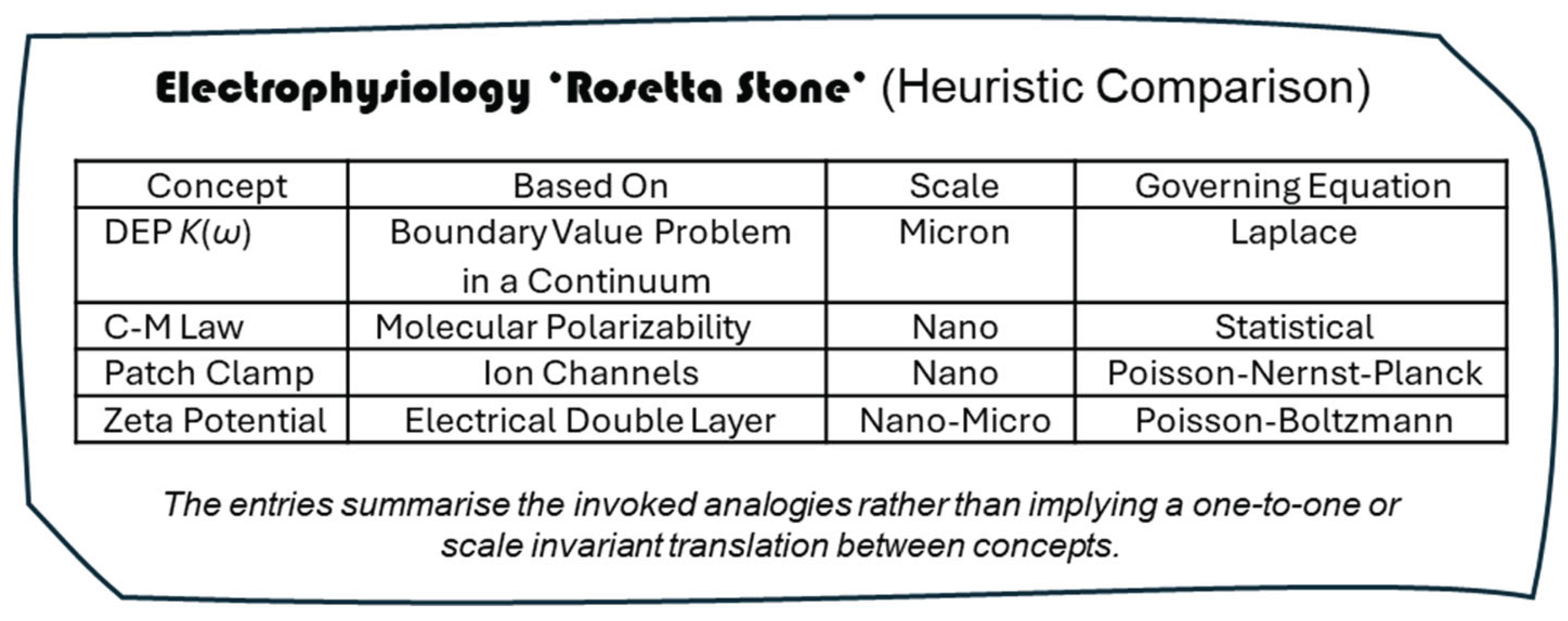
Figure 2.
A plot of the transmembrane field Emem, derived from Equation (13) for an applied local field of 30 kV/m, is shown superimposed on a typical plot of the DEP response for lymphocytes in a medium of conductivity 40 mS/m [57]. The zone where cell bursting is commonly observed is indicated.
Figure 2.
A plot of the transmembrane field Emem, derived from Equation (13) for an applied local field of 30 kV/m, is shown superimposed on a typical plot of the DEP response for lymphocytes in a medium of conductivity 40 mS/m [57]. The zone where cell bursting is commonly observed is indicated.
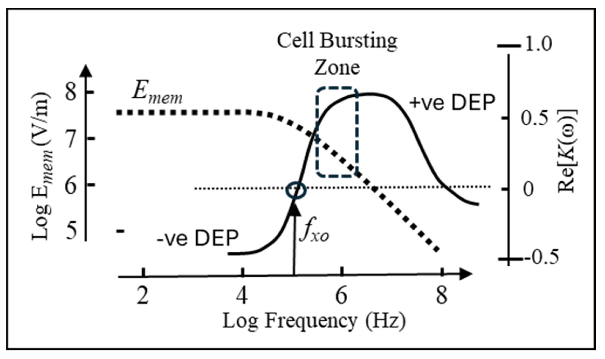
Figure 3.
(a) A periodic function f(t), defined by its location around the circumference of a circle, has a fundamental period T of 2π. (b) The shaded and unshaded regions for show areas where the function is positive or negative, respectively, when wrapped around a sphere.
Figure 3.
(a) A periodic function f(t), defined by its location around the circumference of a circle, has a fundamental period T of 2π. (b) The shaded and unshaded regions for show areas where the function is positive or negative, respectively, when wrapped around a sphere.
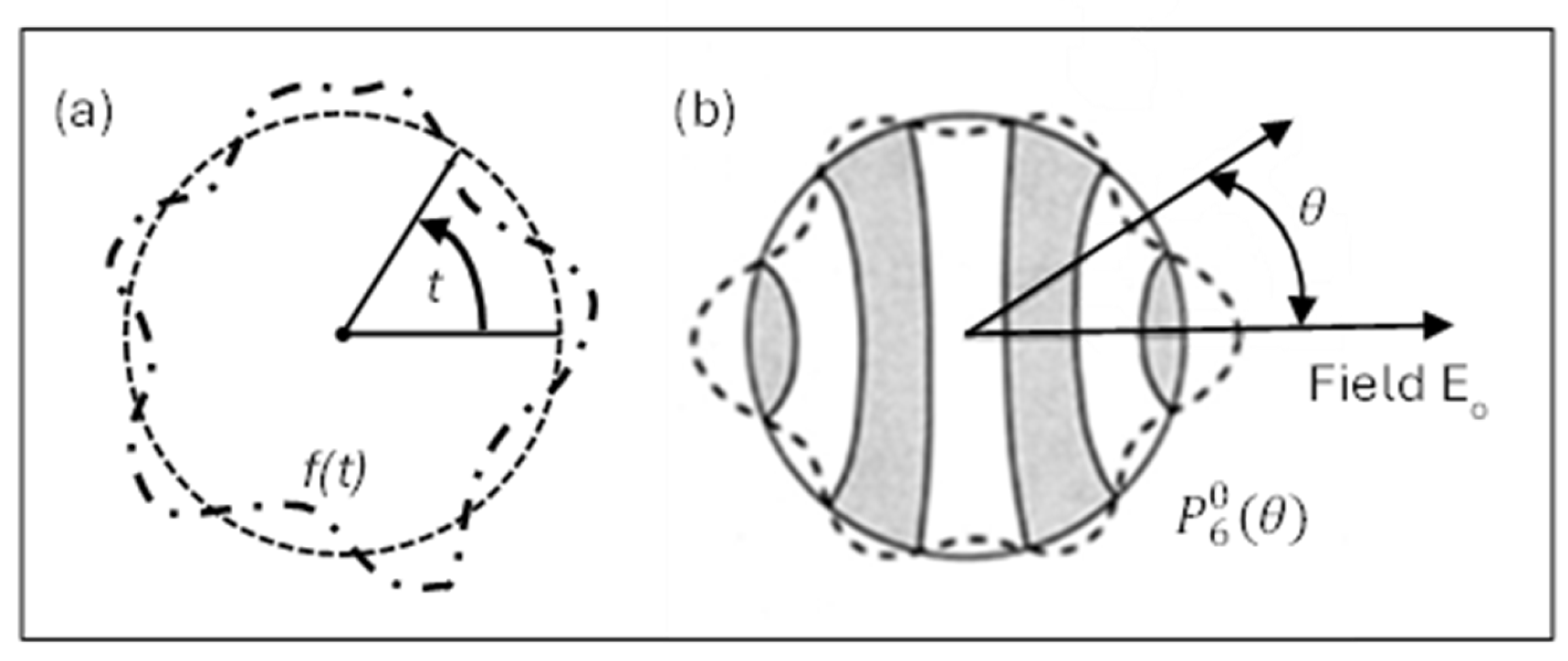
Figure 4.
Experimental scheme to determine the perturbations of flow velocity v, along a tube of diameter D packed with porous material, caused by a spherical inclusion of porosity p and radius R. The hydraulic pressures at points P1 and P2 remain fixed. The Darcy flux q is given by .
Figure 4.
Experimental scheme to determine the perturbations of flow velocity v, along a tube of diameter D packed with porous material, caused by a spherical inclusion of porosity p and radius R. The hydraulic pressures at points P1 and P2 remain fixed. The Darcy flux q is given by .
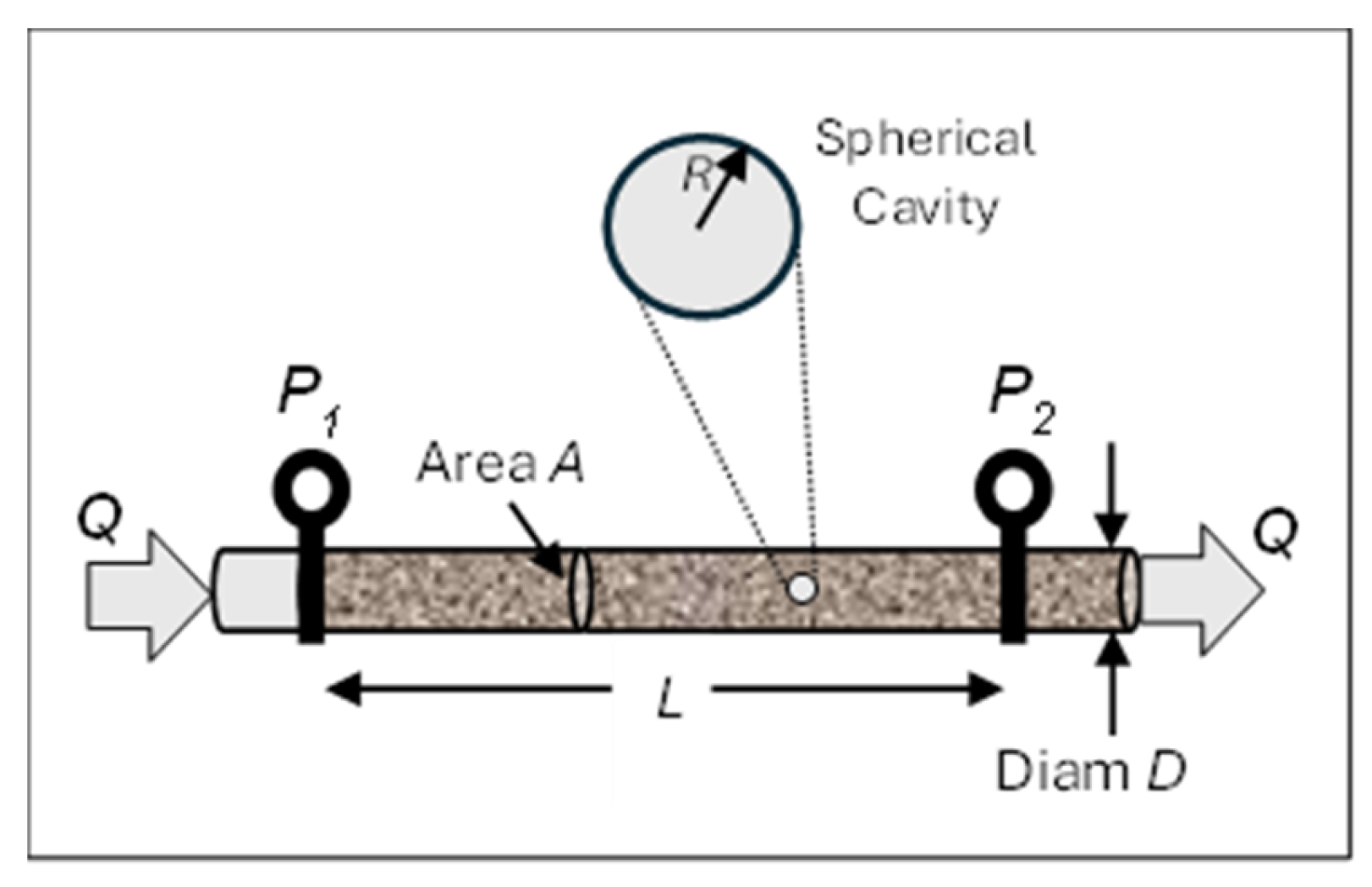
Figure 5.
Pictorial representation of Equation (36). The perturbation on the velocity field is caused by a dipole field, located at the centre of the spherical inclusion, being added to it.
Figure 5.
Pictorial representation of Equation (36). The perturbation on the velocity field is caused by a dipole field, located at the centre of the spherical inclusion, being added to it.
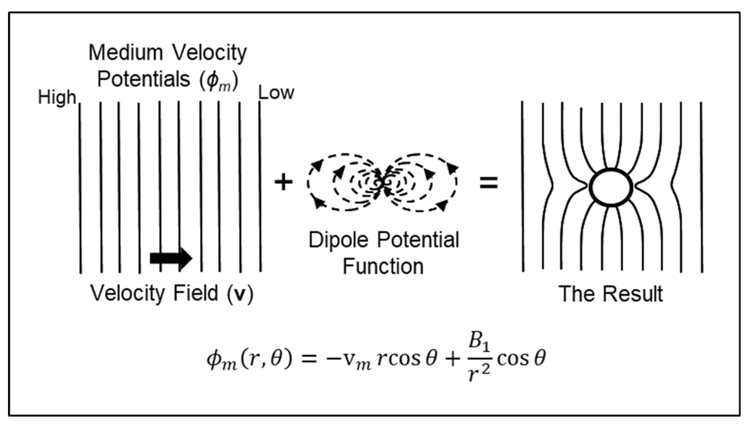
Figure 6.
The boundary conditions used to solve Laplace’s equation for Darcy fluid flow. The spherical inclusion and surrounding material have porosity values pin and pm, respectively. An infinitely thin surface region S bounds the sphere and acts as the boundary with the external material. A vector n is drawn normal to S. (a) The velocity potential functions ϕin and ϕm are continuous across S. (b) The Darcy flux (q = pv) normal to S is continuous across S.
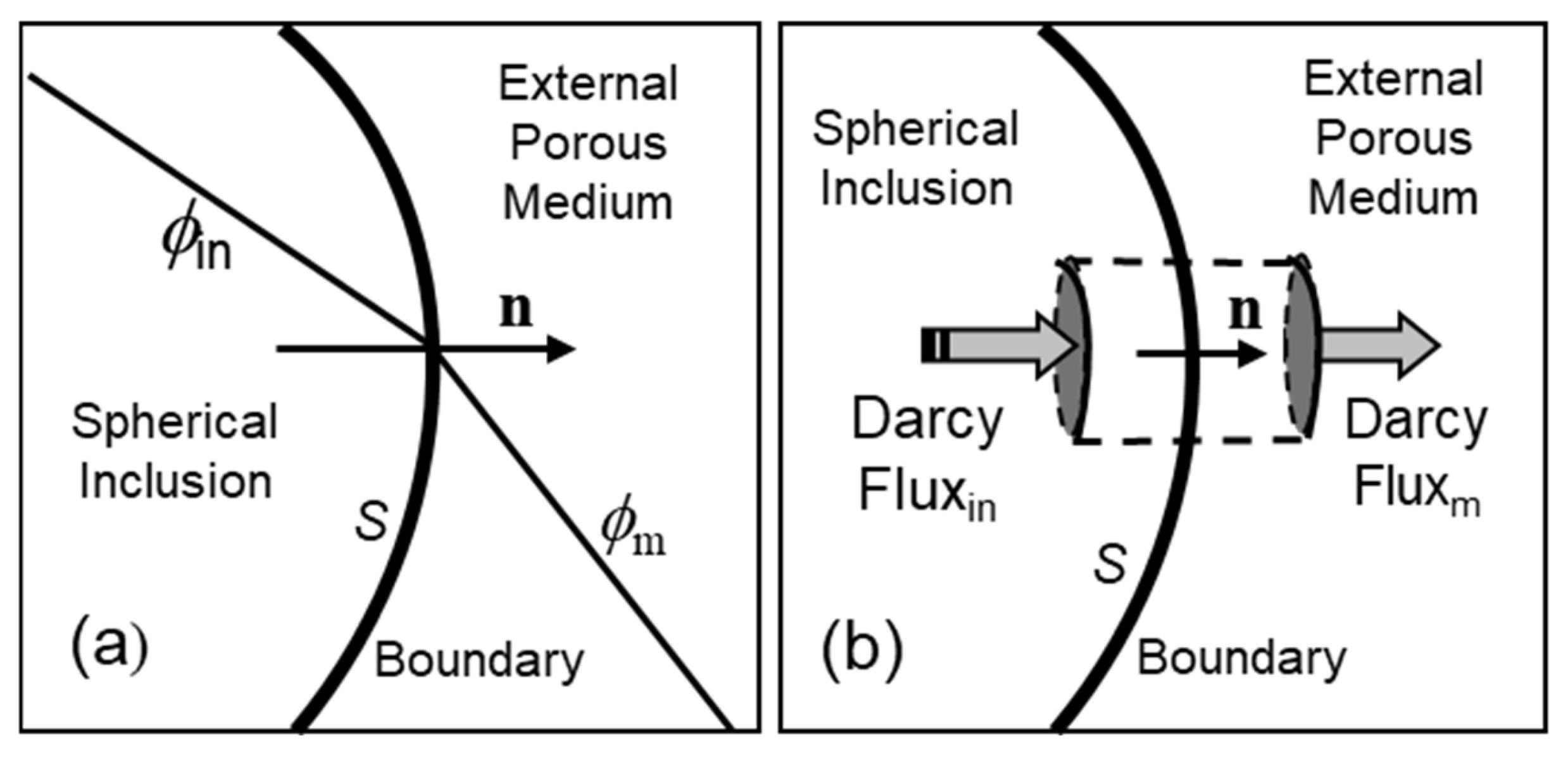
Figure 7.
Perturbation of Darcy flow lines for two values of the K-factor.
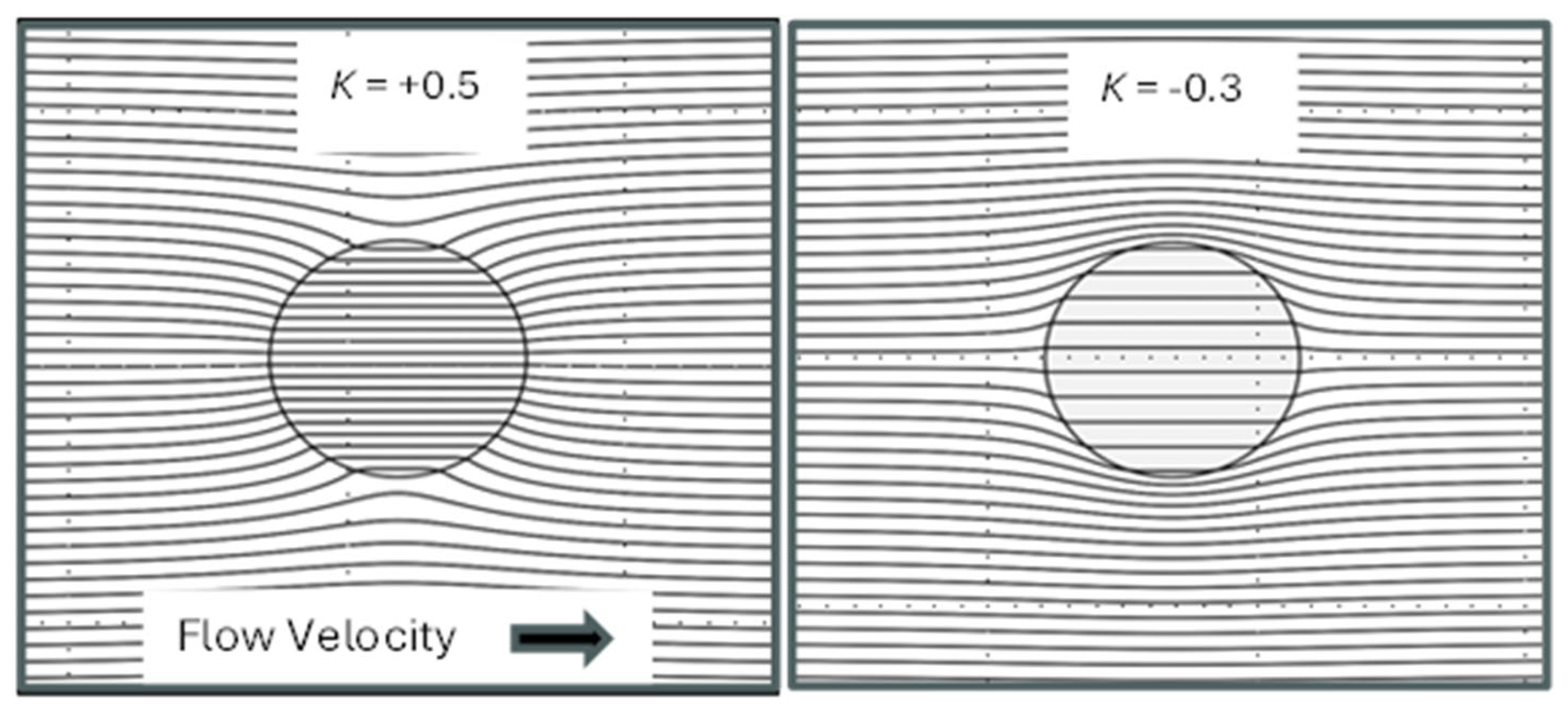
Figure 8.
External and internal magnetic field lines for a uniformly magnetized sphere composed of (a) paramagnetic material (μr = 2.8); (b) diamagnetic material (μr = -0.48). (obtained from Gray (1898) [66, Figs 28 & 29, p.58]).
Figure 8.
External and internal magnetic field lines for a uniformly magnetized sphere composed of (a) paramagnetic material (μr = 2.8); (b) diamagnetic material (μr = -0.48). (obtained from Gray (1898) [66, Figs 28 & 29, p.58]).
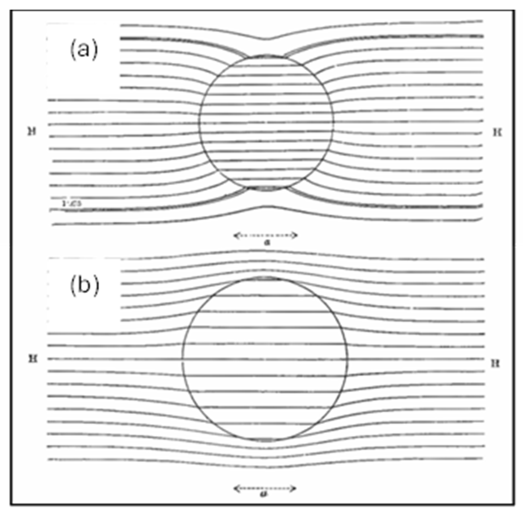
Figure 9.
(a) and (b): Field applied parallel and perpendicular, respectively, to the major axis and minor axis, respectively, of a prolate spheroid. (c): Field applied at 45o to the major axis. A rotational torque is exerted on the spheroid, of magnitude governed by the imaginary component of K(ω).
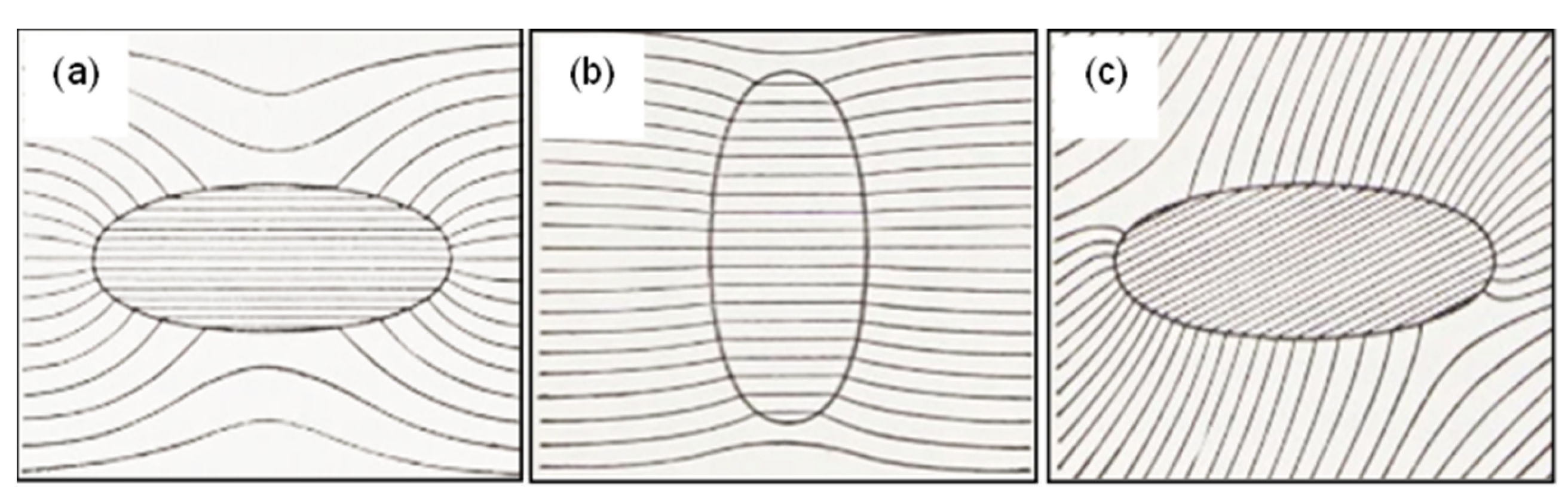
Figure 10.
Left: DEP response of human blood cells before and after neuraminidase treatment. Right: DEP response of erythroleukaemia cells before and after treatment with hexamethylene bisacetamide (HMBA). Treatment reduced membrane surface charge and increased effective conductivity [69].
Figure 10.
Left: DEP response of human blood cells before and after neuraminidase treatment. Right: DEP response of erythroleukaemia cells before and after treatment with hexamethylene bisacetamide (HMBA). Treatment reduced membrane surface charge and increased effective conductivity [69].
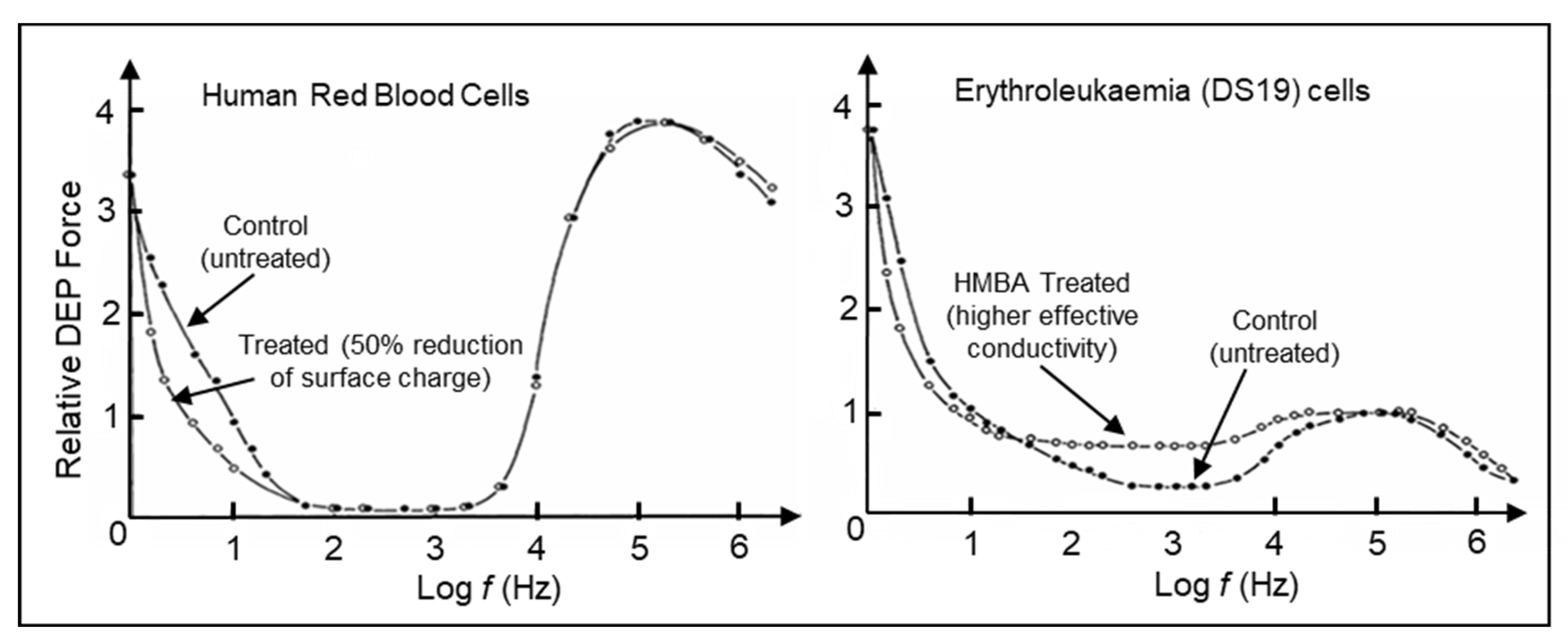

Table 1.
Mossotti provided the qualitative physical picture (corpuscles whose internal charges shift to create dipoles), which Clausius converted into a quantitative microscopic theory by introducing the correct local field, replacing electric fluids with molecular dipoles, and deriving the full polarizability–dielectric relationship.
| Feature | Mossotti (1850) | Clausius (1879) |
| Physical Model | Corpuscles with displaced aether (electric fluid) | Molecular Dipoles + Field Theory |
| Polarization Mechanism | Charge Displacement | Induced & Thermal Dipoles |
| Local Field | Heuristic | First Rigorous form of the Local Field. |
| Mathematics | Semi-Quantitative | Fully Quantitative Derivation |
| Final C-M Relation | Early Form | Modern Clausius-Mossotti Law |
| Concept | Pre-Maxwellian | Post-Maxwellian Electromagnetism |
Table 2.
A compilation of contrast factors, K, that are derived for spherical particles across various topics in physics and engineering. This illustrates the universality of the K-factor form across Laplacian fields.
Table 2.
A compilation of contrast factors, K, that are derived for spherical particles across various topics in physics and engineering. This illustrates the universality of the K-factor form across Laplacian fields.
| Subject | Potential | Property | K-Factor |
| Darcy Flux | Velocity ϕ |
Porosity (a number) p | |
| Conductors | Electric ϕ |
Conductivity (S m-1) σ | |
| Magnetostatics | Magnetic φm |
Permeability (H m-1) μ | |
| Geophysics | Gravitational Φ |
Density (Kg m-3) ρ | |
| Hydrodynamics | Velocity u |
Viscosity (kg m-1 s-1) η | |
| Heat Conduction | Temperature T |
Conductivity (W m-1 K-1) k |
Table 3.
Conceptual parallels between Darcy flow and DEP are shown, with respect to a complex-valued formulation of the contrast factor K(ω).
Table 3.
Conceptual parallels between Darcy flow and DEP are shown, with respect to a complex-valued formulation of the contrast factor K(ω).
| Feature | Darcy Flow | DEP/Dielectrics |
| Driving Potential | Hydraulic Pressure P | Electrical Potential ϕ |
| Flux | Darcy Flux q | Electric Displacement D |
| Loss | Viscous Dissipation | Joule Heating (σ) |
| Storage | Compressibility | Capacitance (ε, Cm) |
| Phase Lag | q lags v | P lags E |
| Imaginary Part | p’’ | ε’’ |
Disclaimer/Publisher’s Note: The statements, opinions and data contained in all publications are solely those of the individual author(s) and contributor(s) and not of MDPI and/or the editor(s). MDPI and/or the editor(s) disclaim responsibility for any injury to people or property resulting from any ideas, methods, instructions or products referred to in the content. |
© 2025 by the authors. Licensee MDPI, Basel, Switzerland. This article is an open access article distributed under the terms and conditions of the Creative Commons Attribution (CC BY) license (http://creativecommons.org/licenses/by/4.0/).
Copyright: This open access article is published under a Creative Commons CC BY 4.0 license, which permit the free download, distribution, and reuse, provided that the author and preprint are cited in any reuse.


