Submitted:
23 December 2025
Posted:
24 December 2025
You are already at the latest version
Abstract
Populations and population dynamics can be understood by the combined interactions of resource supply, demographic pressures, and genetic interactions. In this work, a computational model integrating resource-based population growth and traditional Mendelian inheritance is presented. The modelization of population change over successive generations with a defined sex-based framework and scoring of genotypes (RR, Rr, and rr) is included, and stochastic mating and Poisson-distribution-based birth rate subject to resource interactions are also included in this Python-based computational model. Death rate is a stochastic function of resource use, factoring for age and intergenerational survival probabilities. We will examine the dynamics of the population under a wide spectrum of birth rates, overall resource availability, as well as overall resource utilization per capita under detailed simulations. The findings describe the different regions of collapse, growth, and stabilization phases of evolution along with the shifted high fertility boundary under strong resource conditions. For a scenario of abundant resources and a stable population, we have demonstrated that the genotype distribution tends to a Hardy-Weinberg equilibrium. Additional examples incorporating genetic disorders describe the different evolution patterns under recessive and dominant conditions along with the rapid elimination of dominant deleterious alleles. We also examine the population response to three categories of disasters: moderate, severe, and catastrophic, calculating minimum fertility values for recovery and the number of survivors for each case. Simplified models of single-locus genetics, without mutation or migration, allow for an integrated analytical approach to investigating the interplay of environmental pressure, genetic composition, and demographic processes in shaping population resilience. This research demonstrates the utility of computer simulations in bridging the gap between ecological theory and genetic models of population and also yields fresh approaches to understanding population survival over time, subject to fluctuating environmental pressures.
Keywords:
RCPC
; survival constant
1. Introduction
Populations of living organisms are dynamic systems
which, under the action of some external action, may change [1,2]. such as resource availability, predation, and
environmental conditions-for example, climate change; along with internal
factors like mutations and diseases. Understanding these variations It is
important in ecology, evolutionary biology, and genetics. These factors show
the survivability of a species, and sustainability and balance of an ecosystem.
Naturally, ecosystems, organisms constantly adapt to a change in the
environment. When there is a sudden depression in resources, for example,
competition or drought may lead to a reduced growth rate or an overall decline
in population size [2,3]. Likewise, a sudden
plenty of resources can create a boom, which may be followed by resource
depletion. These dynamics are reflected in population growth curves and reflect
how a species interacts with its surroundings [1,2].
The study of these responses is necessary in that it enables us to predict how
a population might react to different stimuli in its environment.
In the modern ERA, it is possible to carry out
computational modeling and efficiently investigate such scenarios by
computational simulations. this provides a powerful tool for visualising and
analysing the complex interplay between environment, genetics, and increasing
population.
Gregor Mendel founded the basis for our knowledge
in inheritance with his three fundamental laws of inheritance [4]:
- Law of Dominance : When two different alleles are present in an organism, one may mask the expression of the other. The expressed trait is called dominant, while the hidden trait is recessive.
- Law of Segregation :An organism possesses two alleles for a particular trait, which segregate during gamete formation. Consequently, each gamete receives only one allele from each pair, Ensures genetic variation in the offspring.
- Law of Independent Assortment : The alleles of different genes are distributed to gametes independently of one another. Consequently, the inheritance of one trait generally does not influence the pattern of inheritance of another, given that the genes are on dissimilar chromosomes. or are far apart on the same chromosome.
The concepts established the basis of classical
genetics and allowed us to understand how certain traits move. through
generations and how genetic diversity arises in a population.
In the real world, population Studies take decades,
and it is difficult to study or predict populations under different conditions.
(e.g., lack of resources or low genetic diversity) for such a duration of time
(hundreds of Generations are assisted in software modeling, which helps in
simulating, analyzing, and predicting populations across: hundreds or thousands
of generations. It is also possible to do what-if scenario simulations-for
Examples include removal of a genotype or resource shocks—without interfering
with real populations. Hence, such simulations are resource-efficient. This
project attempts to simulate the growth and genetic composition of the
population over several generations using Python. By incorporating Following
Mendelian rules of inheritance combined with models of population growth, the
program traces the evolution of while changing genotype frequencies and overall
population size yield interesting interaction between the genetics and the
demographic factors. Therefore, combining a computational approach with
classical genetics Coupled with the interaction between these diseases and
population dynamics, this project thus presents a framework within which an
analysis of the long-term effects of environmental change and genetic variation.
By bridging the gap between theory and application,
Through better visualisation, we further our understanding of population
dynamics but also play to improve into predictive modeling in evolutionary
biology. Studying these responses is not only about Graphs and data constitute
only a small part; it deals with the living systems and the organisms in
general. share this planet. Each graph tells a story: the rise of a species, or
perhaps its fall, driven by the forces of nature. This is basically where, by
understanding these simulations, we put on nature’s shoes and explore Scenarios
that could take decades to develop.
2. Methodology
2.1. Basis of Population Growth
To study population growth, we require certain
variables and initial data.
2.1.1. Initial Population Data
Sex Ratio The sex ratio of a population is the
number of females per given number of males. For our case, we track the total
numbers of males and females in the population. This is critical, as it can
strongly affect growth trends. For example, if the number of females is very
low relative to males, initial growth will be slow until the difference reduces
and approaches balance.
Genotypic Data We use Mendelian inheritance;
therefore, we require the initial genotype counts to start the simulation:
| RR | Homozygous dominant |
| Rr | Heterozygous |
| rr | Homozygous recessive |
2.1.2. Birth Rate (Natality)
Birth rate is the number of live births for a given
population in a given time period [8]. In our
simulation, we treat the birth rate as the average number of children
produced per mating pair. Birth rate determines how fast a population grows
and how well it can recover from shocks.
*Factors Affecting Birth Rate
- Fertility of the population: Every individual has a reproductive capacity determined by reproductive health. If a greater fraction of individuals are infertile, the birth rate per pair decreases.
- Resource availability: When a population demands more resources than the ecosystem can provide, resources are shared thinly. Individuals receive less than needed to remain healthy, indirectly lowering birth rate.
- Sex ratio: In populations where polygamy is common, a higher number of females allows growth even with fewer males (tending towards a 1:1 ratio). Where polygamy is not common, birth rates collapse if too few pairs can form.
2.1.3. Death Rate (Mortality)
Death rate is the number of deaths in a population per unit time. In our simulation we model death rate as an individual-level probability of death that may depend on external or internal factors [9].
*Factors Affecting Death Rate
- Resource consumption of the population: If the population demands more than the ecosystem can supply, health declines and mortality increases.
- Diseases: Diseases or genetic disorders can significantly increase mortality overall or for specific genotypes.
- Disasters: Stochastic disasters can cause sudden population declines.
2.1.4. Carrying Capacity (K)
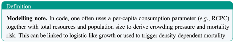
2.1.5. Resource Consumption per Capita (RCPC)
RCPC is the total amount of resources one individual needs to stay healthy and reproduce.
2.2. Assumptions Taken for the Model
- Each Individual has one mate only.
- Generation n will have lower death rates than generation n-1.
- Generation n-2 will die out completely as they are too old to survive.
- Birth rate depends on how much resources are present per individual in the population after reaching carrying capacity it becomes constant.
- Death rate also varies with resource consumption per capita of the population.
- Infant mortality rates, deaths due to diseases, etc are all included in the in death rate of the population.
2.3. Algorithm
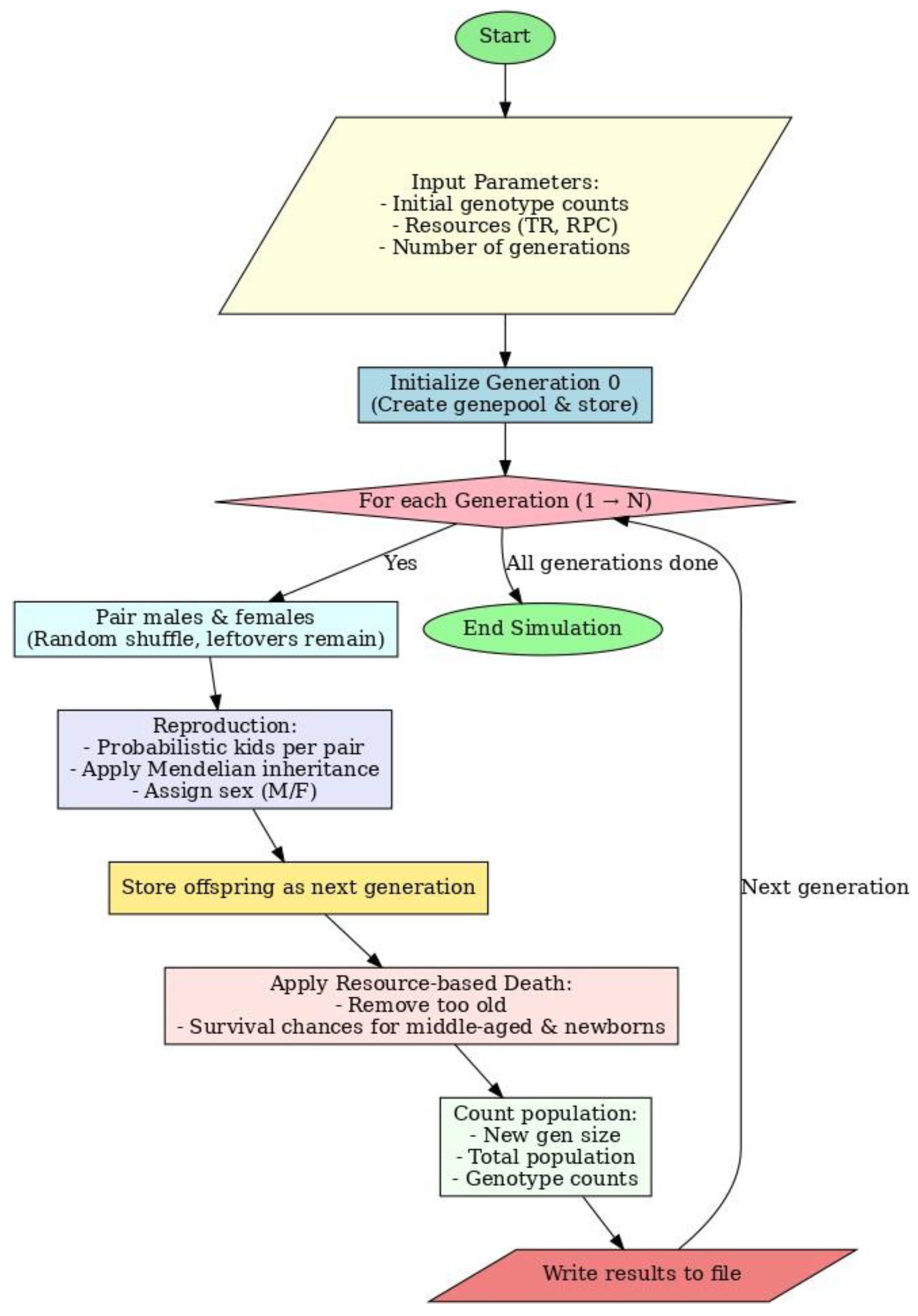
The algorithm starts with population and environment initialization. The program then itera- tively simulates the cycle of pairing, reproduction, and death over multiple generations. New individuals are generated according to Mendelian rules of inheritance each generation, and death is applied probabilistically depending on available resources. The program repeats this cycle to produce realistic growth and decline curves of the population and changes in genotype frequencies.
Figure 1.
Algorithm.
2.4. Input
The simulation takes the following user inputs:
Homozygous dominant males:
Homozygous dominant females:
Homozygous recessive males:
Homozygous recessive females:
Heterozygous males:
Heterozygous females:
Ecosystem system data:
Enter Total resource availability:
Enter resource consumption per individual:
Birth rate:
Enter the number of generations to simulate:
These would be stored in some variables.
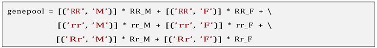
This information is retained in a list of tuples as the genepool. Each tuple has two items: genotype and sex.
For instance:
2.5. Birth Probability Calculation
Birth rate is taken as input from the user. We are considering birth as the average number of offsprings born per mating pair in the population.
The probability of the number of offsprings will be calculated using Poisson’s distribution [7].
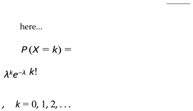
k = average births per mating pair.
λ = number of offspings for which we are calculating probability.
We take maximum k as 8.
Function for the following distribution is:
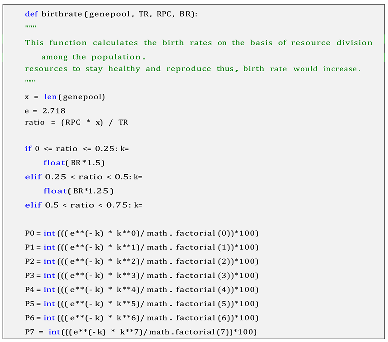
Also we are considering birth rate to be slightly higher when population size is significantly below carrying capacity of the ecosystem. After the population reaches a certain mark the birth rate stabilizes.
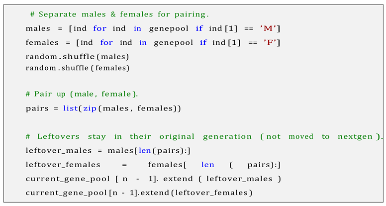
2.6. Pairing
Males and females are sorted into two lists and paired randomly. A male can only pair with one female per generation. Any remaining individuals (excess males or females) are retained in the current generation but do not add offspring in that cycle.
2.7. Crossing
The number of offspring per pair is determined for each pair using a Poisson distribution modified for resource consumption. Probability distribution is computed in the birthrate() function, taking into account both the intrinsic birth rate and the impact of resource availability.
Mendelian inheritance laws are then used to produce offspring genotypes:
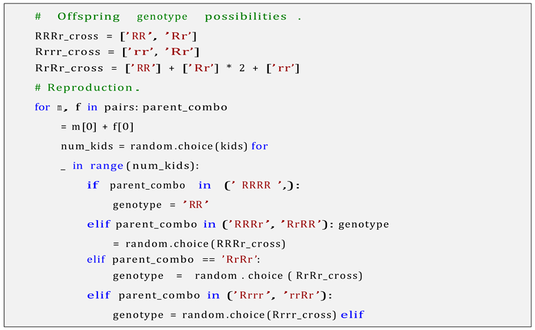
The specific lines of code cover all possible pairs formed and assign sex at random.
2.8. Updation
Updates all the data to the current gene pool:

2.9. Death Rules
- Once reproduction is over, the population experiences mortality due to age and resource utilization.
- Old adults (generation n-2) are eliminated entirely (aging-related death).
- Middle-aged adults (generation n-1) survive probabilistically via the resource() function.
- Newborn adults (generation n) survive by the resource1() function, which provides them with slightly greater survival probabilities than old adults.
Both functions compute death probabilities as a function of the ratio:
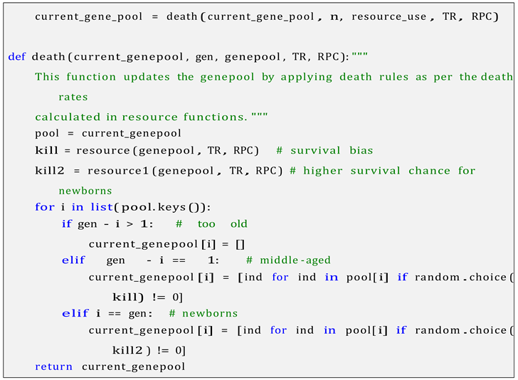
death function scans each individual in the population and kills them at random chance. Which is calculated in the resource function.
2.10. Resource Functions
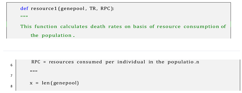
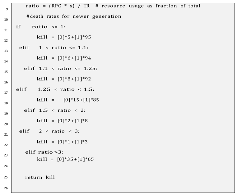
The function returns a list consisting of the probability of death based on resource consumption of the entire population. Where 1 is life and 0 is death.
3. Simulation Observations
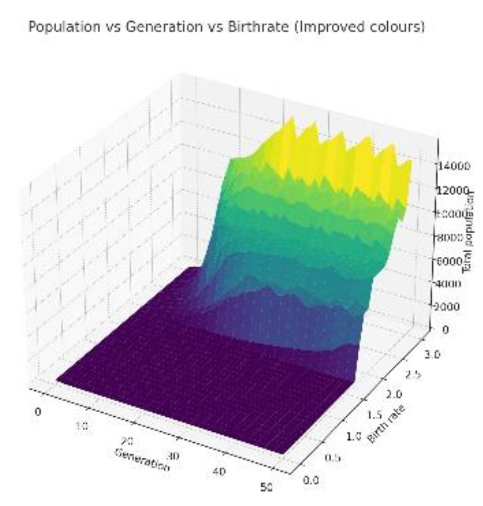
3.1. Variation with Change in Birth Rates
Birth rate is one of the most important factors that influence how fast a population can increase, recover from damage, or collapse due to environmental pressure[2,8]. In contrast to an independent variable, birth rate has close interplay with other ecological parameters like available resources, carrying capacity, and resource consumption of resources. Under ample resources, populations can maintain higher birth rates, resulting in exponential growth. In contrast, in cases of resource scarcity, pressures for survival limit reproduction and can push populations towards decline or equilibrium.
Observation of variations with birth rate gives us an idea of how the populations evolve and get stabilized over generations. If one simulates populations with varying reproductive parameters, then it is possible to see the equilibrium between genetic inheritance, resource limitation, and mortality effects.
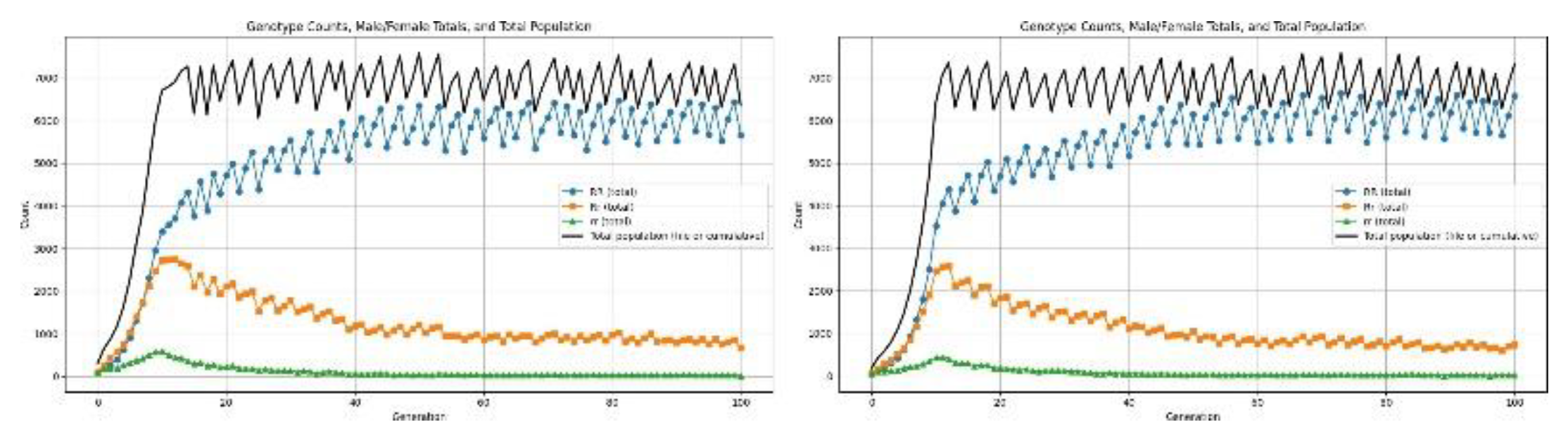
We begin with a population of 60 individuals, distributed evenly across the three genotypes (20 RR, 20 Rr, and 20 rr) with an equal sex ratio (30 males and 30 females). The carrying capacity is set at 200,000 units, providing sufficient space for natural interactions and population dynamics. Each individual consumes 20 resource units (RCPC), establishing the baseline for resource limitation in the system. Using this setup, we systematically vary the birth rate from 0 to 3.0 in order to analyze how changes in reproductive potential influence population growth, genotype distribution, and long-term stability. The following graphs show the results we get by running these simulations.
Figure 2.
For birth rates 1.7 and below.
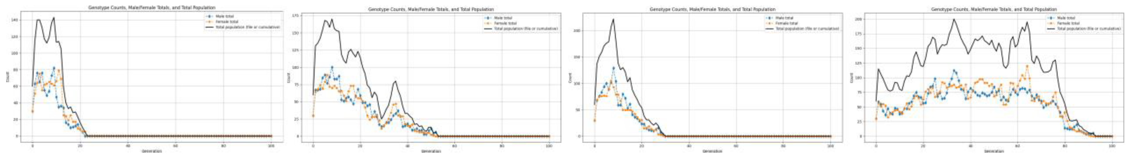
Figure 3.
For birth rates 1.8 and above.
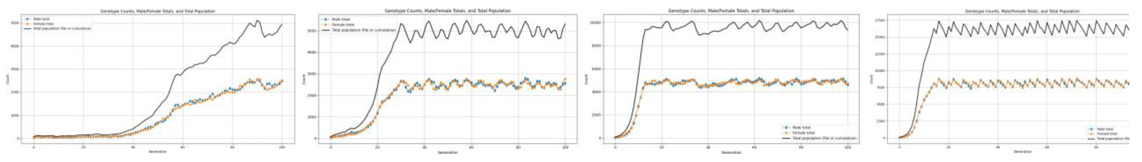
Figure 4.
Figure shows how gradient of growth changes with change in birth rate.
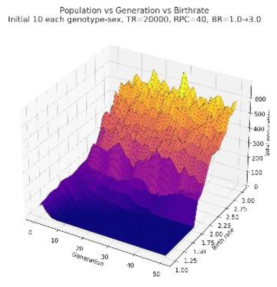
3.2. Low Resources
We model extreme ecological stresses—famines, resource collapses, and scarcity-driven population bottlenecks—by manipulating the total resource availability parameter, TR, to considerably lower values[10,21]. In these simulations, TR is generally reduced to 20,000–25,000 units, representative of environments in which carrying capacity is severely constrained. In order to assess how resource scarcity interacts with individual energy demands, we vary resource consumption per capita—RCPC—across two contrasting regimes: Low-RCPC conditions (20 units) to study populations adapted to minimal per individual consumption, and Higher-RCPC conditions (50 units) to model populations with higher metabolic or ecological demands. All other initial population and genetic parameters are kept identical between simulations so that any divergence in population dynamics is due to resource limitations and their interaction with RCPC.
Figure 5.
3d plot showing how population behaves in absence of abundant resources.
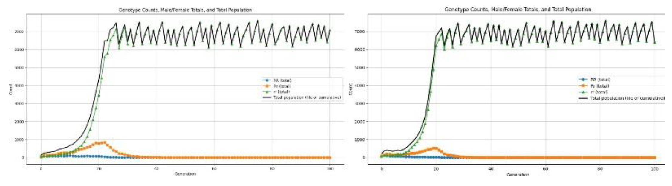
3.3. Genotypic Variation Observations
Genotypic Variation Observations We observe that, across the simulated generational timeline, the change in genotype frequencies due to differential fertility, survivability, and resource-mediated selection pressures shows distinct patterns[11,12]. These emerge from the interplay between Mendelian inheritance, genotype-specific fitness effects, and environmental constraints such as resource limitation.
Figure 6.
Graphs showing genotypic frequency with population growth.
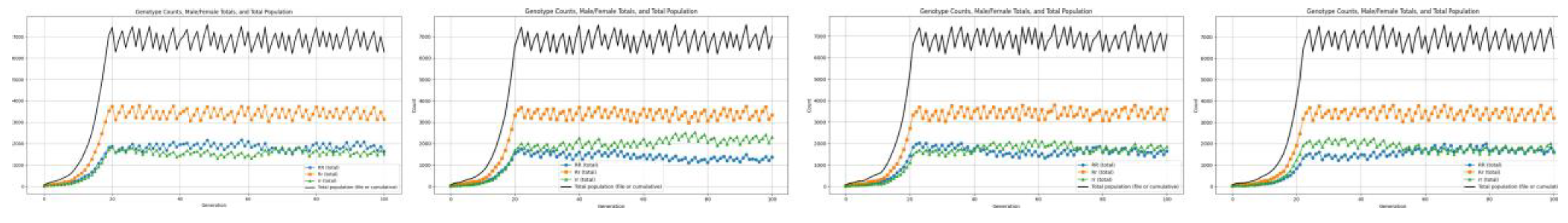
Figure 7.
Graph showing average of 20 simulations for genotypic analysis.
3.4. Defective Genotypes
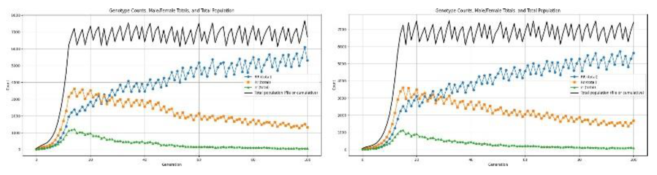
3.4.1. Reproductive Disorder
Recessive Disorder: This class of genetic disorders manifests when the dominant allele is absent; that is, the disorder is phenotypically expressed only in homozygous recessive individuals. In the present simulation this recessive defect is operationalized as a reduction in fertility specifically for individuals with the homozygous recessive genotype (rr). We simulate population dynamics across 100 generations to assess the long-term demographic consequences of this reproductive impairment. These trajectories permit us to describe the effects of recessive fertility loss on population growth, genotype frequency shifts, and overall stability of the system.
Figure 8.
Results for recessive allele causing low fertility.
Dominant disorder: This class of genetic disorders is expressed whenever at least one copy of the dominant allele is present. Unlike recessive conditions-which require homozygosity for manifestation-dominant disorders affect both heterozygous (Rr) and homozygous dominant individuals (RR). In this simulation, the dominant defect is expressed as a fertility reduction that is applied to all individuals carrying the dominant allele without respect to zygosity. Hence, both the RR and Rr genotypes have poor reproductive success, but the homozygous recessive genotype (rr) retains its normal fertility. We simulate here the demographic and genetic dynamics over 100 generations to investigate the long-term, population-level impact of such a dominant fertility impairment. This allows us to observe characteristic patterns in population growth, shifts in allele frequencies, and potential selection pressures acting against the dominant allele.
Figure 9.
Results for dominant allele causing low fertility.
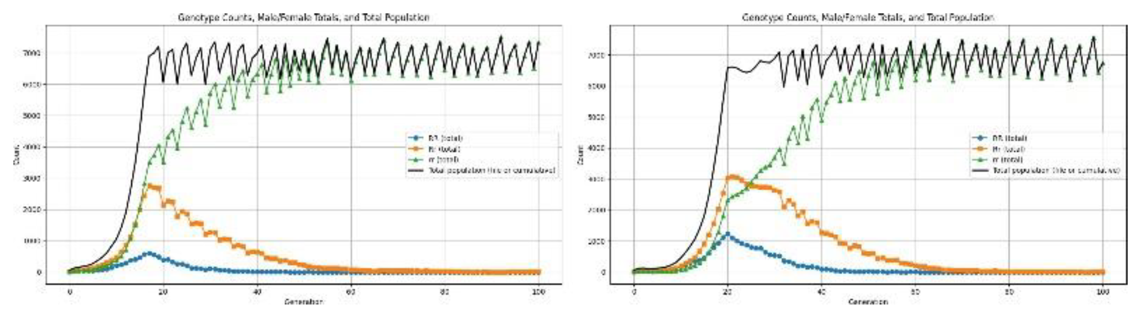
3.4.2. Health Disorders
Health disorders are genetic conditions that lower the survivability of the individuals who bear them, and thus affect demographic outcomes and the course of allele-frequency change. In the present framework, health-affecting defects are modelled by changes in mortality rates, operating at the survival-selection stage of every generation.
Recessive Health Disorder: This disorder is only phenotypically expressed when an individual is homozygous recessive (rr). Individuals who are carriers of the defective allele, in heterozygous form, continue to be unaffected, Rr. In this model, the disorder is implemented as increased mortality risk for rr individuals, reducing their probability of surviving to reproductive age.
Figure 10.
Results for recessive allele causing low survivability.
Dominant Health Disorder: Dominant health defects always appear when an individual has at least one copy of the dominant allele: thus, both heterozygous (Rr) and homozygous dominant (RR) individuals are equally affected. Here, in the simulation, those genotypes are given a heightened chance of death in the survival-selection step, while the only rr individuals are unaffected. By incorporating these mortality-based impairments into the process of updating generations, we can observe how health disorders reshape survivability, stability of the population, and the dynamics of allele-frequencies across 100 simulated generations.
Figure 11.
Results for dominant allele causing low survivability.
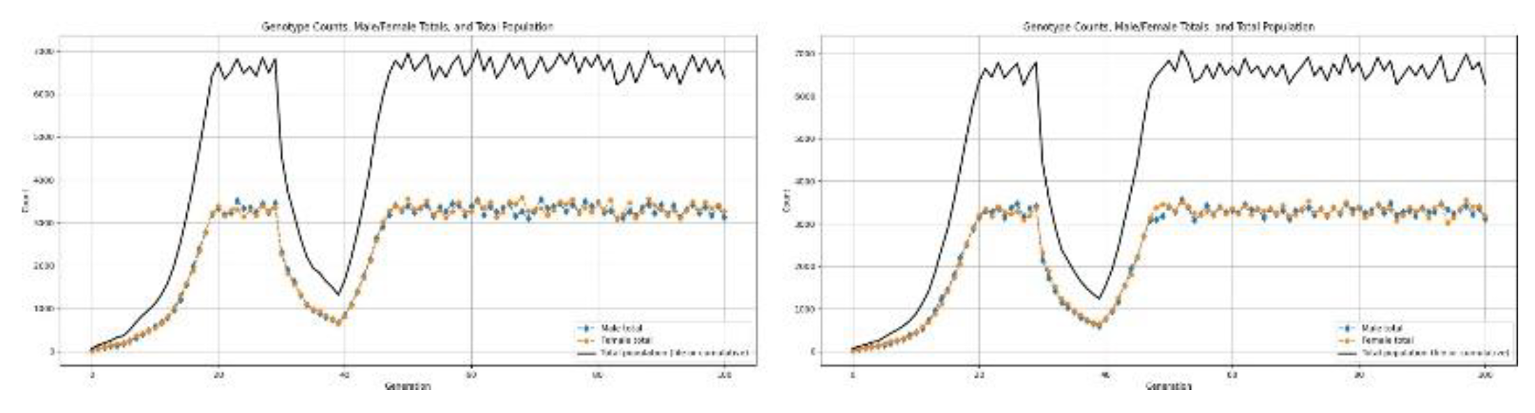
3.5. Disasters
3.5.1. Type-1 Disaster: Moderate Collapse
Mortality:30–40 percent of the population is eliminated.
Duration: Lasts about 10 generations, thus enabling cumulative, long-term stress on population recovery.
Biological/Ecological Examples:
- -
- Multiyear regional droughts
- -
- Long-term crop failures resulting in chronic famine.
- -
- Prolonged disease endemics with moderate lethality—for example, historical waves of malaria or cholera.
- -
- Sustained environmental degradation: soil nutrient loss, habitat fragmentation Type-1 events mimic chronic but not catastrophic pressures—enough to significantly reshape population structure over many generations.
Figure 12.
Results for population undergoing a type-1 disaster.
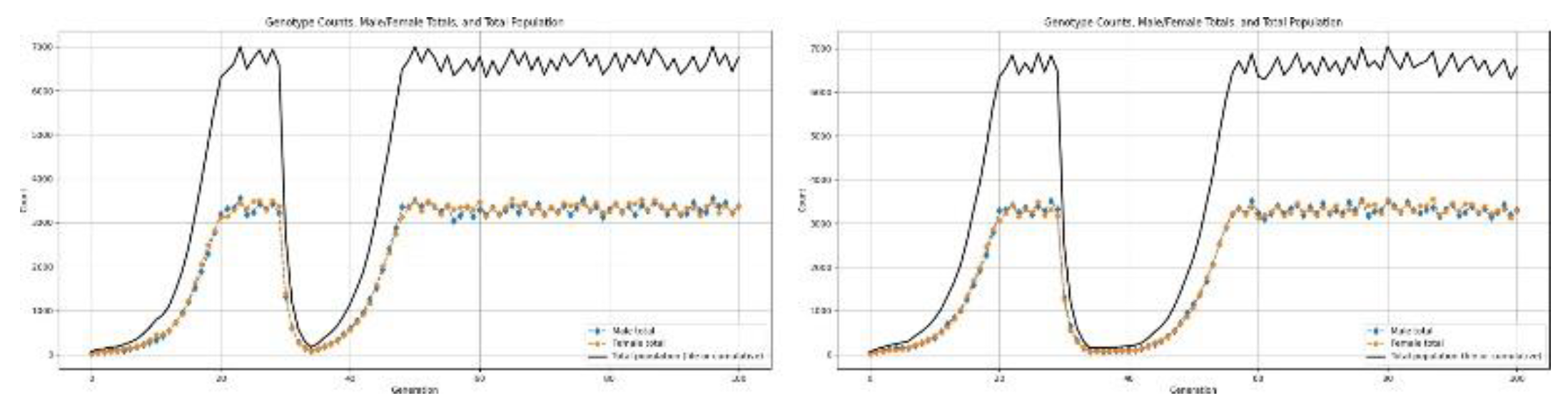
3.5.2. Type-2 Disaster: Severe Collapse
Mortality: The mortality rate is characterized by the sudden death of about 60 percent of the population.
Duration: It lasts 4–5 generations, thus creating a pronounced demographic bottleneck. Biological/Ecological Examples:
- -
- Sudden climate changes, such as rapid cooling or multicontinent monsoon failures
- -
- Highly lethal infectious disease outbreaks, such as smallpox or measles in immunolog- ically naïve populations
- -
- Large-scale wildfires or volcanic eruptions affecting multi-year resource availability
- -
- Oceanic or freshwater ecosystem crashes; i.e., fishery collapses, oxygen depletion events Type-2 disasters exert extreme selective pressure and can accelerate changes in allele frequencies.
Figure 13.
Results for population undergoing a type-2 disaster.
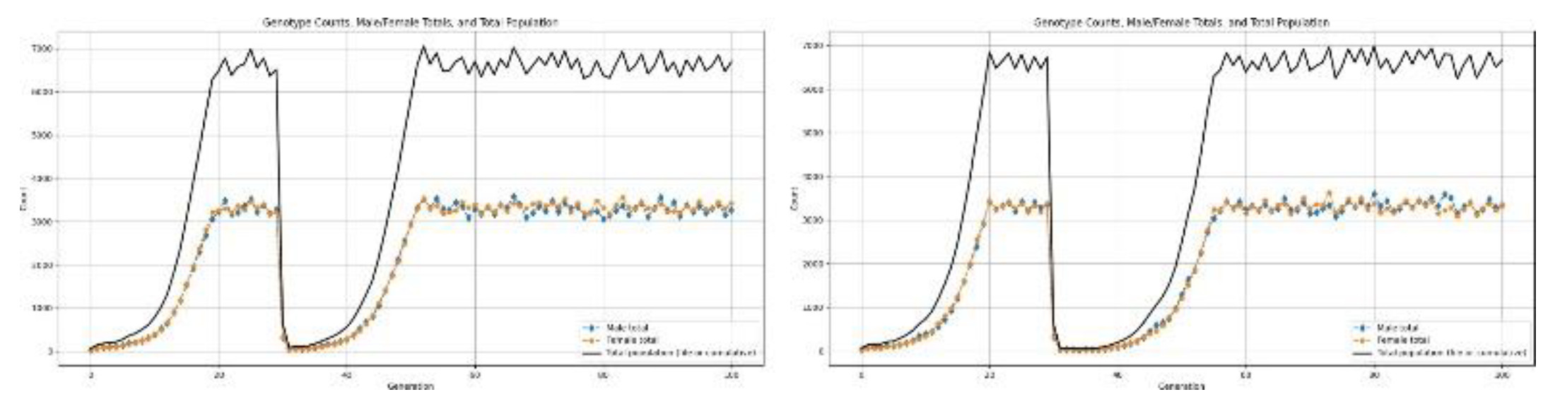
3.5.3. Type-3 Disaster: Catastrophic Collapse
Mortality: About 90 percent of the population die within one generation. Duration: 1 generation only, the event being sudden, catastrophic, and short-lived. Biological/Ecological Examples:
- -
- Meteor impact or massive volcanic eruption causing near-instant ecosystem collapse
- -
- Super-virulent pandemics with extreme lethality
- -
- Acute toxic contamination events (Chemical spills, Radiation exposure)
- -
- Sudden habitat elimination: tsunami, large-scale glacier melt floods Type-3 disasters are near-extinction events and often determine whether a population survives at all.
Figure 14.
Results for population undergoing a type-3 disaster.
4. Results and Discussions
4.1. Population Collapse for Lower Birth Rates
At low birth rates-roughly =< 1.7-1.8-the population has an initial growth phase due to the initial favorability of resource availability and low mortality from density dependence[2,8]. However, it is not sustainable for the long term. Resource limitation begins to escalate as population size increases, resulting in increased mortality and decreased effective reproduction. Subsequently, it ends in a population collapse.
With the simulation framework, we can estimate the time to collapse defined as the generation at which the population size declines irreversibly below a viable threshold. This allows us to quantify how long populations can persist under subcritical birth-rate regimes and to compare collapse dynamics across different environmental and genetic scenarios.
We can estimate after how many generations population collapse occurs and how it depends on the following variables:
- -
- Nt: Population size at generation t
- -
- N0: Initial population
- -
- TR: Total available resources
- -
- RPC: Resource consumption per capita
- -
- BR: Birth rate
- -
- µ(λ): Average number of children produced per pair
- -
 : Resource usage ratio
TR
The total population in the next generation depends on:
- Survival of existing individuals, given by probability Sold(λ)
- Survival of newborn individuals, given by probability Snew(λ)
- Average reproduction — each pair produces on average µ(λ) offspring. Since only half of the population can breed (assuming equal sexes), the fraction of new offspring relative to the total population is 1 .
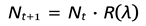
The total population in the next generation is directly proportional to the population in the previous generation:

Hence, population dynamics can be expressed through a survival constant R(λ), defined as:
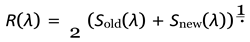

Here R(λ) can be termed as the average of survivablity of both older and younger generations including the new born individuals of the population, it gives us as idea about the survival of the entire population in general.
This leads to the recurrence relation:
- -
- If R > 1, the population grows or survives.
- -
- If R < 1, the population shrinks and eventually collapses to extinction.
Also R(λ) is not constant for throught the time period a population exists but changes as λ changes for the population. ∴ It cannot be defined for the population but for the population at a specific time.
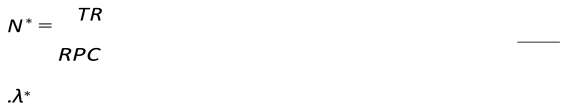
The number of generations until the population falls below one individual can be estimated as:

4.2. Stable Phase
We can observe that in simulation for birth rates above a certain threshold the population grows exponentially and eventually stabilizes at a certain level. Using the model we can estimate this stabilizing zone for any population.
A population will stabilize when its birth rate or the number of offsprings produced in a given time is equal to the death rate[24]. If we were to describe it in terms of R(λ) it is the time when R(λ) for population is approximately equal to one.
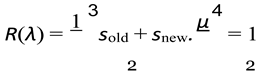
Here:
- -
- sold(λ) is a function that depends on λ and defines the survivability for older genera- tions.
- -
- snew(λ) is a function that depends on λ and defines the survivability for younger generations.
- -
- µ(λ) is a function that depends on λ and defines the birth rate of the population.
Let λ* be the solution for R(λ) = 1.
Now the number at which the population will stablize can be given as:
4.3. Birthrate as a Function of λ
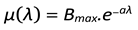
However for our model due to computational limitations we use a discrete function of birthrate variation with λ we can represent µ as an exponential function of λ.
We know that fertility(birth rate) decreases exponentially as the population more and more resource pressure.
Therefore we can write:
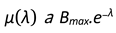
Here Bmax is the maximum birth rate the population can achieve. Also the different types of environments and species can lead to different kind of dependence on λ which means the sensitivity to change in resource pressure can be different in each case. For this we define a sensitivity constant a which can be introduced in this equation as:
4.4. Behavior in Absence of Abundant Resources
Populations evolving under these parameter regimes are designed to approximate con- temporary human populations under high resource pressure. In natural systems, these conditions are typically characterized by much more demographic stability at the lower fertility rates, where the slower rate of population increase creates less strain on finite resources. At very high fertility rates, population growth should be rapid enough to quickly exceed ecosystem carrying capacity, and resource depletion, mortality, and—due to the assumed exponential dependence of mortality rate (µ) on resource pressure—the effective fertility rate should decline markedly.
However, this behavior, empirically expected, is not fully reproduced by the present model. On the contrary, the simulations show a larger stability of populations for higher birth rates, even under conditions of constrained resource availability. This is most likely the result of structural simplifications in the model, especially in how resource pressure feeds back to fertility and mortality dynamics.
Even with this limitation, this model does provide an essential insight: with severe resource scarcity, the minimum fertility rate needed to maintain a viable population is much higher than under resource-abundant or baseline conditions. This shift in the critical fertility threshold underlines how environmental stress can fundamentally alter the demographic requirements for population persistence.
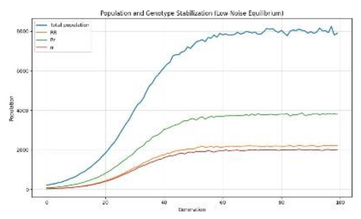
4.5. Genotypic Analysis
This not only constitutes a strong basis against which internal consistency and biological plausibility can be measured for population-genetic models but also allows the assessment of the genuineness and reliability of model outcomes through the examination of whether simulated genotype frequencies conform to theoretically established expectations.
In this regard, we have done 20 independent runs of the simulation under the condition of plentiful resources and a fixed birth rate of 2.5 offspring per mating pair. For these runs, the total population stabilizes at an average of 8098 individuals. The corresponding genotype distributions converge to mean values of around 3756 heterozygous individuals, 2261 homozygous dominant individuals, and 2081 homozygous recessive individuals.
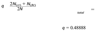
Let:
- -
- p = frequency of the allele R.
- -
- q = frequency of the allele r.
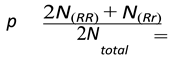
Also:
p = 0.51111
Now if we were to calculate p2 + 2pq + q2 using these values of p and q.
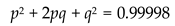
Which is approximately equal to 1.
This implies that the genotype frequencies given by the model satisfy the Hardy–Weinberg equilibrium, as expected for large, randomly mating populations in the absence of selection, mutation, or migration. We can therefore conclude that under resource abundant and demographically stable conditions, the model yields classical population-genetic behavior similar to that seen in real biological populations.
4.6. Genetic Disorders
4.6.1. Reproductive Recessive
A genetic disorder that manifests in the absence of the dominant allele R is called a recessive disorder. Such disorders decrease the reproductive fitness of the affected indi- viduals by reducing fertility by a specified factor. A typical case is Congenital Hypogo- nadotropic Hypogonadism (CHH)[15], an autosomal recessive disorder due to the deficiency of gonadotropin-releasing hormone secretion (GnRH). This hormone deficiency causes impaired gonadal function, thus leading to lower fertility both in males and females.
These are modeled, in the simulation framework, by reducing the fertility of homozygous recessive individuals selectively (rr) while keeping the heterozygous (Rr) and homozygous dominant individuals (RR) unchanged. Over successive runs of simulation, the population shows growth and stabilization according to theoretical expectations from recessive fitness impairments.
Under these conditions, the homozygous-dominant genotype is the most frequent, but the heterozygous genotype (Rr) reaches a stable frequency and the homozygous recessive genotype is driven to very low—but nonzero—frequencies. Thus, it will never be completely eliminated from the population.
The persistence of the recessive allele provides a mechanistic explanation for the prevalence of recessive genetic disorders in natural populations. Affected individuals have reduced fertility, but the defective allele is preserved via heterozygous carriers who are phenotypically normal and continue to pass the allele to the next generation.
Quantitatively, after many simulation runs, the stable genotype counts converged to an average of about 5872 homozygous dominant individuals, 918 heterozygous, and 87 homozygous recessive individuals, with the total population stabilizing around 6877 individuals. These results align with established population-genetic principles that attend to the recessive disorders and how alleles persist due to carriers.
If we were to calculate p and q for the stable phase of such simulation. We get:

and
4.6.2. Reproductive Dominant
Dominant reproductive disorders are a class of genetic disorders that manifest phenotyp- ically in the presence of the dominant allele R. Such conditions lower the reproductive fitness of affected individuals due to reduced fertility in all genotypes carrying the dominant allele R; this includes both heterozygous and homozygous dominant individuals, which can be represented as Rr and RR, respectively.
An illustrative example is autosomal dominant hypogonadotropic hypogonadism[16], a disorder characterized by disrupted development and impaired signaling of gonadotropin- releasing hormone-producing neurons. The disruption further leads to reduced gonadal function and, therefore, lower fertility in both sexes.
For this disorder, the simulation framework uses the application of a fertility reduction to all carriers of the dominant allele, while homozygotes for the recessive allele (rr) are not affected. When the simulation has been run repeatedly, there is a characteristic evolutionary trajectory for the population: selection acts strongly and directly against the dominant allele, leading to its progressive decline and eventual elimination from the population.
Equilibrium is reached where the population settles to a point where only the recessive allele exists and the dominant allele is completely extinct. This result emphasizes the key distinction between dominant and recessive fertility-reducing defects: dominant defects are always exposed to selection, but recessive defects can pass through heterozygous carriers to subsequent generations.
4.6.3. Health recessive
Recessive health disorders these are genetic disorders that get expressed in the phenotype only if the individual does not possess the dominant gene, that is, only in homozygous recessive individuals (rr). These disorders impair biologic fitness by reducing survivability, which means that the chances of survival for the individual until reproductive maturity are reduced.
A classic example is Phenylketonuria (PKU)[14], which is an autosomal recessive metabolic disorder due to the loss of function of the enzyme Phenylalanine hydroxylase. PKU, if not managed through dietary means, causes an accumulation of toxic metabolites, thereby causing development retardation and mortality.
In the simulated framework, recessive health disorders are represented through an increase in the homozygous recessive mortality rate, with heterozygous (Rr) and homozygous dominant (RR) individuals unaffected. This reproduces real-world simulations of recessive health disorders.
In particular, the population approaches stability for similar ranges of demographics, with the number of homozygous recessive persons censused being drastically reduced though the recessive gene is not totally wiped out. This is also due to the preservation of the defective gene in carrier heterozygotes, protecting it from selection.
4.6.4. Health Dominant
Dominant health disorders refers to the diseases that appear if an organism is carrying at least one dominant allele. This means that both heterozygous individuals with the genotype of Rr and homozygous dominant with the genotype of RR are regarded as having the health disorder. These disorders pose a threat to biologic fitness by causing low survivability rates, often leading to death before the reproductive age.
Dominant health disorders are simulated in the framework using a high mortality rate for all individuals with the dominant allele in the homozygous recessive state (rr), while individuals with the homozygous recessive state remain unaffected by health issues. Due to the influence of selection on the dominant allele in each generation, the selection pressure is strong.
In the repeated simulations, there is a clear and direct evolutionary outcome for the population. The gene frequency of the dominant allele diminishes quickly through the generations and eventually becomes extinct in the population. At the point of equilibrium, the population ends up with only the recessive allele, where all the individuals in the population are homozygous recessive.
This is in contrast to the type of dynamics that is observed for recessive health disorders, in which the deleterious allele is allowed to segregate via heterozygotes. The lack of any such refuge in dominant health disorders is what creates the purging of the deleterious allele, which is exemplary of the principal role of dominance in determining the persistence of the allele.
4.7. Disasters
4.7.1. Type-1
This kind of disaster creates a harsh demographic bottleneck[11], hence applying a strong selective pressure on the population. Unlike sudden extinction events, in this case, a reduced population is achieved over a protracted but prolonged period, hence sufficient time for selection to become cumulative over a series of generations.
Such simulations indicate that in order for our numbers to successfully begin a recovery and sustained presence in these circumstances, a stable rate of procreation of 2.5 children per reproductive pair would be required. Furthermore, our calculations indicate that at the end of this global disaster, there would be 500 million human beings on this planet.
A theoretical rate of birth of 2.0 or perhaps a fraction lower may perhaps be sufficient to preserve population numbers under ideal circumstances with minimal selective pressure on a species and plenty of available resources. Taking into consideration other practical requirements in a post-disaster setting, population density will most likely be low, with a minimal remnant population scattered geographically and socially in very small groups. This leads to a reduction in effective mating population size, thus impacting reproductive efficiency[12,13].
4.7.2. Type-2
Type-2 disasters exhibited a more severe demographic bottleneck due to a larger rate of decline of the population than in the case of Type-1 events. Stronger intensity of mortality over shorter timescales applies exceptionally high selective pressures, causing a very rapid decrease in population size and genetic diversity.
These parameters and outcomes of simulation studies suggest that, in such conditions, the human populations are able to avoid extinction and achieve their long-term persistence only at birth rates no lower than at least 3.0 offspring per mating pair. At lower levels of fertility, the population decline is rapid and irreversible, considering the combined effects of high mortality, reduced effective population size, and intensified selection.
By quantifying the simulation trajectories below, we estimate that in the wake of a Type-2 disaster, the human population would decline to as low as 32 million individuals. Recovery after the disaster is further hindered at such low population sizes by extreme population fragmentation, limited availability of mates, and increased stochastic effects[17,18] .
Accordingly, a birth rate of at least 3.0 is the practical demographic threshold needed to overcome the combined effects of a high mortality rate, decreased connectivity among the remaining groups, and environmental stress persisting during the aftermath of a Type-2 disaster.
4.7.3. Type-3
This class of disaster involves an extremely steep and rapid decline in the population, which results in an extreme demographic bottleneck over a very short time. The intensity of mortality and sudden loss of population impose very strong selective pressures that severely constrain recovery potential during an immediate post-disaster period.
The results of the simulations suggest a minimum stable birth rate of about 2.8 offspring for every mating pair is essential for a human population to successfully survive such a bottleneck event. If it were less than this, continued decline in population is expected due to the small effective population size with its associated higher stochastic mortality and restricted mating opportunities.
This consideration yields, according to the quantitative analysis, a conservative estimate that, in the wake of such a disaster, the number of humans surviving would fall back to about 80 million. In such a small population size, population fragmentation and reduced connectivity among surviving groups further hinder demographic recovery and increase the fertility threshold required above the normal rate for long-term persistence.
4.8. Limitations
Although it has produced important results concerning population and genotypic dynamics under varying environments and genotypes, among other aspects, some of the drawbacks of the current model are below:
Computational Constraints as
The model will not be able to realistically reproduce a very large population size due to the constraint of resources and processing capacity. The model will not be able to simulate over a very large number of generations because the long-term evolution will definitely be understated.
Single-Gene Inheritance Framework
The model is limited by single-locus, two-allele inheritance, which is a greatly simplified representation of the genetics of natural populations. Complex traits with multiple genes, epistasis, and polygenic selection are not accounted for.
Limited Accuracy Under Extreme Resource Pressure
Resource-dependent fertility and death rates are incorporated into this model, but under very high resource pressure, it fails to correctly model real population dynamic behavior. This is because simplified cycles of resource depletion, death rates, collapsed fertility, and recovery are not incorporated into this model.
Mutation Absence and Evolutionary Innovation. The above model does not take into consideration the role of mutation, gene flow, or adaptive evolution. Therefore, this model will not be able to incorporate new alleles and will not show any eventual evolution based on selective pressure. Such deficiencies suggest a slew of future considerations, including better scaling algorithms, multilocus genetics, evolution processes, and resource demography couplings.
Acknowledgments
I would like to express my sincere gratitude towards Yatin Prakash and Skanda D Bhaskar for their valuable recommendations regarding the project. Also I would like to express my gratitude towards Sutirth Dey for recommending reading material that contributed to this project.
References
- Verhulst, P. F. (1838). Notice sur la loi que la population suit dans son accroissement. Correspondance Mathématique et Physique, 10, 113–121.
- May, R. M. (1976). Simple mathematical models with very complicated dynamics. Nature, 261 (5560), 459–467. https://doi.org/10.1038/261459a0. [CrossRef]
- Fowler, C. W. (1981). Density dependence as related to life history strategy. Ecology, 62 (3), 602–610. https://doi.org/10.2307/1938559. [CrossRef]
- Mendel, G. (1866). Experiments on plant hybridization. Verhandlungen des Natur- forschenden Vereins in Brünn, 4, 3–47.
- Hardy, G. H. (1908). Mendelian proportions in a mixed population. Science, 28 (706), 49–50. https://doi.org/10.1126/science.28.706.49. [CrossRef]
- Weinberg, W. (1908). Über den Nachweis der Vererbung beim Menschen. Jahreshefte des Vereins für Vaterländische Naturkunde in Württemberg, 64, 368–382.
- Kendall, D. G. (1949). Stochastic processes and population growth. Journal of the Royal Statistical Society: Series B, 11 (2), 230–282. https://doi.org/10.1111/j.2517- 6161.1949.tb00023.x. [CrossRef]
- Dennis, B., Munholland, P. L., & Scott, J. M. (1991). Estimation of growth and extinction parameters for endangered species. Ecological Monographs, 61 (2), 115–143. https://doi.org/10.2307/1943211. [CrossRef]
- Lande, R., Engen, S., & Sæther, B.-E. (2003). Stochastic population dynamics in ecology and conservation. Ecology, 84 (9), 2267–2274. https://doi.org/10.1890/02-0399. [CrossRef]
- Cohen, J. E. (1995). Population growth and Earth’s human carrying capacity. Science, 269 (5222), 341–346. https://doi.org/10.1126/science.269.5222.341. [CrossRef]
- Nei, M., Maruyama, T., & Chakraborty, R. (1975). The bottleneck effect and genetic variability. Evolution, 29 (1), 1–10. https://doi.org/10.1111/j.1558-5646.1975.tb00807.x. [CrossRef]
- Frankham, R. (1995). Effective population size/adult population size ratios in wildlife. Genetical Research, 66 (2), 95–107. https://doi.org/10.1017/S0016672300034455. [CrossRef]
- Lynch, M., & Lande, R. (1998). The critical effective size for a genetically se- cure population. Animal Conservation, 1 (1), 70–72. https://doi.org/10.1111/j.1469- 1795.1998.tb00228.x. [CrossRef]
- Blau, N., van Spronsen, F. J., & Levy, H. L. (2010). Phenylketonuria. The Lancet, 376 (9750), 1417–1427. https://doi.org/10.1016/S0140-6736(10)60961-0. [CrossRef]
- Seminara, S. B., et al. (1998). The GPR54 gene as a regulator of puberty. The New England Journal of Medicine, 349 (17), 1614–1627. https://doi.org/10.1056/NEJMoa035322. [CrossRef]
- Layman, L. C. (2013). The genetic basis of gonadotropin-releasing hormone deficiency. Nature Reviews Endocrinology, 9 (10), 569–576. https://doi.org/10.1038/nrendo.2013.147. [CrossRef]
- Allee, W. C. (1931). Animal aggregations. The American Naturalist, 65 (699), 191–204. https://doi.org/10.1086/280363. [CrossRef]
- Courchamp, F., Clutton-Brock, T., & Grenfell, B. (1999). Inverse density de- pendence and the Allee effect. Trends in Ecology & Evolution, 14 (10), 405–410. https://doi.org/10.1016/S0169-5347(99)01683-3. [CrossRef]
- Kimura, M. (1983). The neutral theory of molecular evolution. Nature, 302 (5903), 546–550. https://doi.org/10.1038/302546a0. [CrossRef]
- Brook, B. W., Traill, L. W., & Bradshaw, C. J. A. (2006). Minimum vi- able population sizes and global extinction risk. Science, 312 (5772), 397–400. https://doi.org/10.1126/science.1127855. [CrossRef]
- Tilman, D., Isbell, F., & Cowles, J. M. (2014). Biodiversity and ecosystem functioning. Annual Review of Ecology, Evolution, and Systematics, 45, 471–493. https://doi.org/10.1146/annurev-ecolsys-120213-091917. [CrossRef]
- Willi, Y., Van Buskirk, J., & Hoffmann, A. A. (2006). Limits to the adaptive potential of small populations. Annual Review of Ecology, Evolution, and Systematics, 37, 433–458. https://doi.org/10.1146/annurev.ecolsys.37.091305.110145. [CrossRef]
- Melbourne, B. A., & Hastings, A. (2008). Extinction risk depends strongly on factors contributing to stochasticity. Nature, 454 (7200), 100–103. https://doi.org/10.1038/nature06922. [CrossRef]
- Lee, R. (2003). The demographic transition. Journal of Economic Perspectives, 17 (4), 167–190. https://doi.org/10.1257/089533003772034943. [CrossRef]
- Bradshaw, C. J. A., & Brook, B. W. (2014). Human population reduction is not a quick fix. Proceedings of the National Academy of Sciences, 111 (46), 16610–16615. https://doi.org/10.1073/pnas.1410465111. [CrossRef]
Disclaimer/Publisher’s Note: The statements, opinions and data contained in all publications are solely those of the individual author(s) and contributor(s) and not of MDPI and/or the editor(s). MDPI and/or the editor(s) disclaim responsibility for any injury to people or property resulting from any ideas, methods, instructions or products referred to in the content. |
© 2025 by the authors. Licensee MDPI, Basel, Switzerland. This article is an open access article distributed under the terms and conditions of the Creative Commons Attribution (CC BY) license (http://creativecommons.org/licenses/by/4.0/).
Copyright: This open access article is published under a Creative Commons CC BY 4.0 license, which permit the free download, distribution, and reuse, provided that the author and preprint are cited in any reuse.


