Submitted:
22 December 2025
Posted:
24 December 2025
You are already at the latest version
Abstract
The ionospheric conductivity is an important variable determined by the mobility of the charged particles and it also dependent of the plasma, neutral number of densities and charged particles. The ionosphere has advantages to absorb the harmful radiation from the Sun for all radio communications, navigation and surveillance transmissions through it. Temperature, cloudy and precipitations are the most factors to determine the wave mobility in the ionosphere region. The conductivity of the three selected districts depends on the altitude variation during day and night time. At altitudes of about 80 to 5000 km there is a flow of a number of current systems. This study was analysis the daily, monthly and seasonal contour variations of ionospheric conductivity in selected districts with their geographic latitude and longitude value. The wave conductivity was vary and increase throughly for the selected Models of Hall, Pederson and parallel conductivities with height and time variability of the ionospheric conductivities, cloudy and the precipitation was analysed with temperature variation for each districts.
Keywords:
ionospheric conductivity
; solar radiation
; geographical latitude
; temperature variation
; altitude variation
1. Itroduction
The upper region of the atmosphere, which is made up of a mixture of the charged and neutral gases between approximately 50 to 2000 km above the Earth’s surface is the Earth’s ionosphere. And useful for all radio communication,navigation and surveillance transmissions through it. By ompassionate the Earth’s ionosphere are associated deciphering the many changes in neutral and plasma density and their relationships to the coupling with the Earth’s lower atmosphere, the generation and flow of currents with in the region of the magnetosphere. To understand these challenges we may observe the composition and dynamics of the neutral particles and charged particles, as well as the particles field-aligned current describing the coupling of the ionosphere to the magnetosphere. This description of the process affecting the ionosphere and thermosphere regions to enhance coupling with the regions below and above at smaller spatial and temporal scales (Menk et al., 1999; Raeder et al., 2001; Toth et al., 2005; Heelis and Maute, 2020). In the ionosphere at altitudes of about 80 to 500 km there is a flow of a number of current systems (Yamazaki and Maute, 2016). This current is a perpendicular current and the field aligned currents flow parallel to the Earth’s magnetic field lines to connect the magnetospheric currents with polar ionospheric currents (Ridley et al., 2006). The ring current involved in the magnetosphere-ionosphere coupling and it flows near dusk in the equatorial magnetosphere to connect the ionosphere with the field-aligned currents and closed in the ionosphere via the ionospheric current system. The most ionospheric current systems are controlled by solar wind pressure and interplanetary electric fields, which makes the variation of geomagnetic activities (Menk et al., 1999). Most magnetic perturbations are produced by ionospheric currents and the electrons are magnetized and strongly bound to the Earth’s magnetic field (Richmon, 1979; Hardy et al., 1985; Heelis and Maute, 2020). A planet’s ionosphere is an ionized upper layer of its atmosphere. If the host planet has a magnetosphere, the ionosphere serves as a coupling between the atmosphere and magnetosphere, transferring energy and momentum. Traditionally, an ionosphere is thought to consist only of positive ions and electrons. The wave conductivity is an important variable determined by the mobility of the charged particles and it also dependent of the plasma, neutral number of densities, Page 1 charged particle gyro-frequencies and their collision frequencies with neutrals. In lower ionosphere, the conductivity provides the propagation of extremely low frequency (0.003-3kHz) and very low frequency waves (Salem et al., 2016). At E-region the plasma is produced at daytime by solar EUV radiations and the conductivity is perpendicular to the magnetic field to largest and the F-region plays an important role to the ionospheric conductivity with plasma transport (Nagai et al., 2003, Wang et al., 2011, 2012; Qian et al., 2014). Ionospheric plasma is generated energetic ultraviolet solar radiation and particle precipitation at high-latitudes. The current flow path is perpendicular to the magnetic field to indicate electromagnetic, gravitational, collision and plasma pressure gradient forces, which are applied on the plasma density (Jin et al., 2011). This flow of current is the spatial distribution the source current and the ionospheric conductivity (Siscoe and Maynard, 1991; Siscoe et al., 2013).
2. Model and Methods
In this study we used the ionospheric conductivity model (height profile) of the World Data Center for Geomagnetism, Kyoto for understanding the height profiles of the parallel, Pedersen and Hall conductivity and their variability of daily, monthly and seasonal profiles over selected area ionosphere during a high and low solar activity phases. The study was analysis the daily, monthly and seasonal profile variations of ionospheric conductivity in selected districts with geographic latitude and longitude 9°48′N 38°44′E.
Both height and time variability of the ionospheric conductivities will be considered to analysis this study. The model for this will be conduct by ionospheric conductivity profile on the variation of the parallel, Pedersen and Hall conductivity.Those are more preferable to identify the longitudinal variation for wave conductivity at different region (D,E,F regions) of atmospheric layer.
Parallel, Pedersen and Hall conductivity, methods are used to determine the number of particle per electron mass with its velocity and they depend on the time duration and wave disturbance at each region .
And other model be used to detrmine the parallel conductivity per cyclotron frequencies with its velocity shown as.
The effective Pedersen conductivity of the ionosphere is found by equating the Ohmic dissipation dissipation with the thermal power transfered from the warmer electrons to the neu-tral gas.
From the viewpoint of the electrons this is the cooling rate. Models for the rates due to different reactions are summarized by Schunk and Nagy (2000, Chapter 9.7). Observations by the EISCAT Svalbard radar show that electron temperatures T in the cusp electrojet reach up to about 4000 K. The heat is tapped and converted from plasma convection in the near Earth space by a Pedersen current that is carried by electrons due to the presence of irregularities and their demagnetising effect. The heat is transfered to the neutral gas by Collisions and the Pederson conductivity peaks at higher altitudes of approximately 130-150 km.
Nextly, we to analyize the parallel conductivity for multiple of electron collission per cyclotron frequency and Hall conductivity peaks at altitudes below 120 km [Richmond and Thayer, 2000].
From Equations (i, ii and iii) the values of and are expressed as follows:-
Those the three methods are combined together to analysis the ionospheric conductivity during high solar activity with the maximum and minimum height variation for each selected district. After all data is accumulated the data will be analyzed by the MATLAB software in case of display the output of the input variable by tabulate as graphical representation
3. Result
Solar radiation, which varies over multiple temporal scales, modulates remarkably the evolution of the ionosphere. The solar activity dependence of the ionosphere is a key and fundamental issue in ionospheric physics, providing information essential to understanding the variations in the ionosphere and its processes. Over recent years, the solar activity effects of the ionospheric parameters have received renewed interest, and considerable progress has been achieved. It is essential to predict the solar activity accurately, especially the trend of the sunspot cycle. Nowadays, popular prediction approaches include the neural network approach, similar-cycle method, empirical orthogonal decomposition, and wavelet analysis. The thermospheric temperature varies with the level of solar activity, which is reflected with electron density profiles.
3.1. Day and Monthly Variability on Ionospheric Conductivity of Fitche
The Pedersen, parallel and Hall conductivities, as well as the magnetic field parameters, are computed. The conductivities in this study were calculated with the concerned duration of ion density at selected day, date, month and year.
The figure below shows that the ionospheric conductivity for the two months of January and the march month was recorded Siemen metric for Hall, Pedersen and Parallel as maximum
as the altitude increase from 100km to 150km the hall value increase from to and become decrease from to as the altitude increase finally it reach the maximum value at 343.75km but for march month it reach the maximum peak than the January and the Pedersen value also increase from 100km to 150km altitude and the decrease for the altitude value changed from 150km to 176.21 km , then it increase slightly with altitude increase and parallel become slightly increase. Due to the variation of time and month the Hall, Pedersen and parallel conductivity are varied.
Figure 1.
Daily and monthly change on ionospheric conductivity of Fiche district.
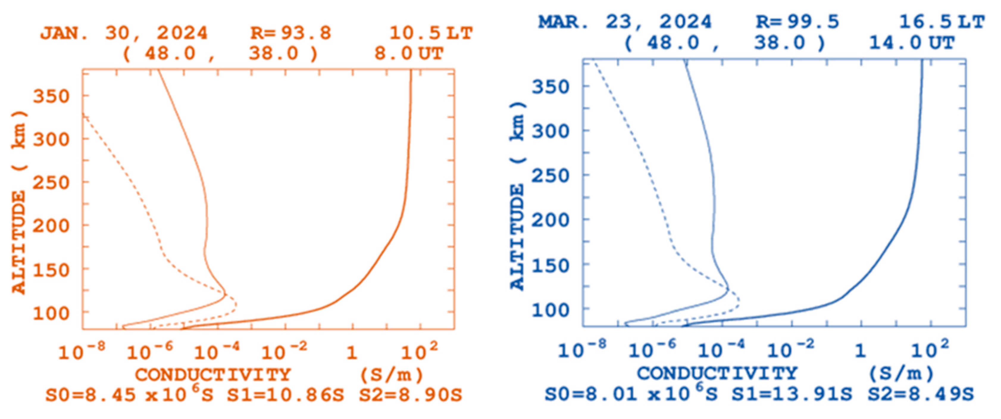
This shows that the ionospheric conductivity for this district is more than the Degem district and less than the Debre Libanos district. Depending on the time variation the solar activity is also varied with the time which mean by the solar activity is high during day time and low during night time. This action indicate that particles are at rest at midnight and the particles are on motion at day time due to this factor time variation cause variability of ionospheric conductivity.
3.2. Effect of Seasonal Change on Sunshine
Solar activity is one of the factors to control the ionospheric conductivity for all region of the ionosphere. Thus, factors are dependable of time variation throughout the year. The sun shine duration through the seasons and months were recorded from the Ethiopian meteorology institute with at constant time of 18:00UT.
The maximum and the minimum value of the shine duration are shown as from figure above. So from this recorded data the entropy or wave disturbance for the maximum at February and the minimum at July and august of 2023.During the sun shine particles are more movable and this time is very important for particle transport and information should be carried out at this time. From below figure at the point 2, 3, 4, and 11 the data was not visible from the institute which mean by at these months there is no recorded data at the institute. For more explanation the serial number on horizontal line of starting from 1 up to 12 represents months of the year as starting from January to December respectively.
Figure 3.
Seasonal Change on Sunshine for fitche district.
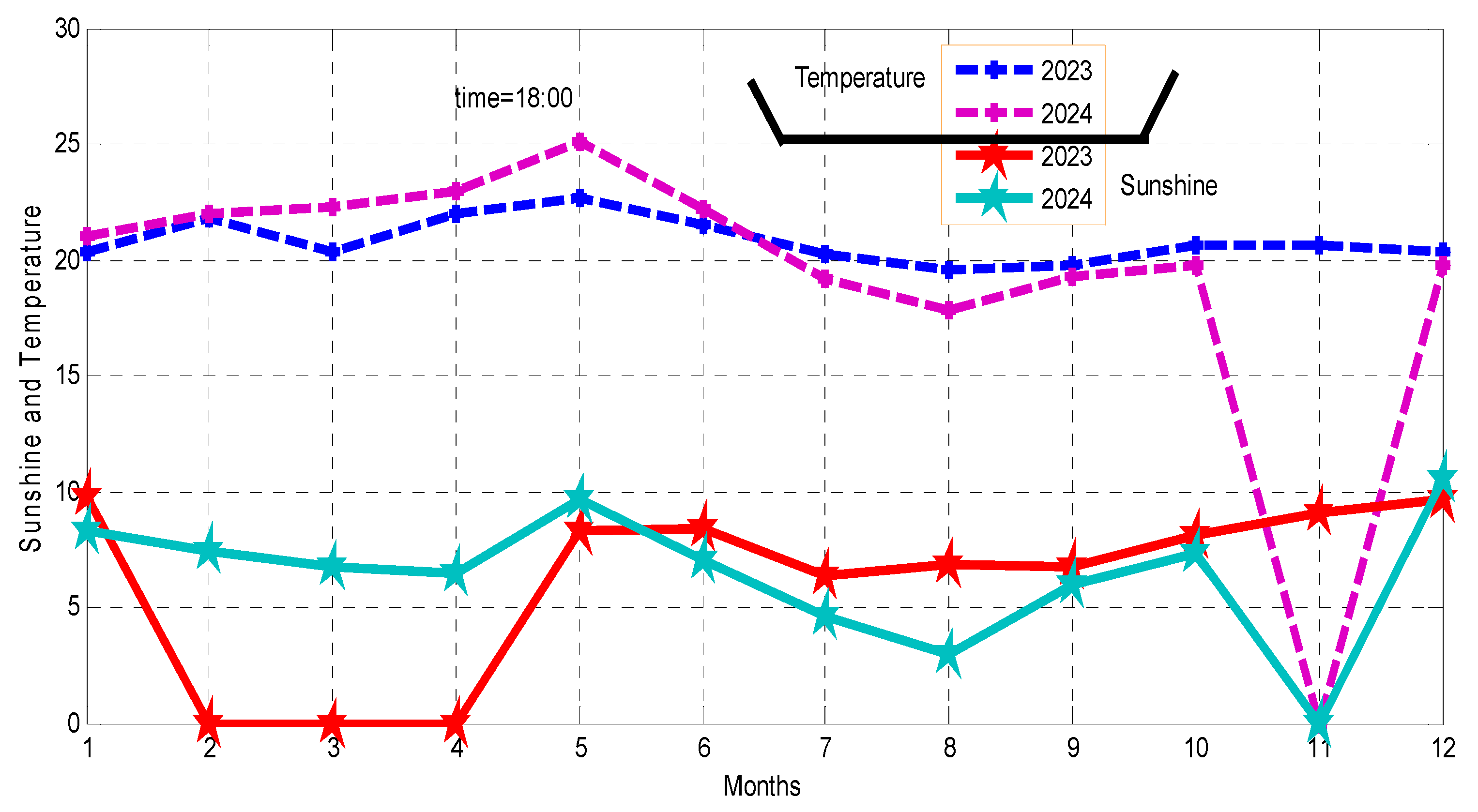
Therefore the points on 2, 3,4,and 11 are shows the values of February, march, April and November. The sun shine become reach the maximum peak point at 11 and reach at the minimum point at 3 in 2024 and the figure above shows as for 2023 it has maximum value at 9 and the minimum value at 2. The sunshine and temperature value is related to each other from the above figure the temperature reach the maximum value 20K and 15 for 2023 and 21K and 20k in 2024. The maximum and the minimum temperature value and the sunshine value of the fitche district are not far apart or nearly the same. So it shows as the fiche district sunshine and the temperature is constant weather condition.
3.3. Temperature Variability on Cloudy and Precipitation of Degem
Temperature, sunshine, cloudy and precipitation are depend on the variability of altitudes. It is obviously, the temperature and altitudes are interrelated to each other as inversely proportional from the three selected districts the Degem district is at high land. The figure below show that the temperature, sunshine are become slightly decrease from January to December months of the year
Figure 4.
Monthly variability on Cloudy and precipitation Change on Degem.
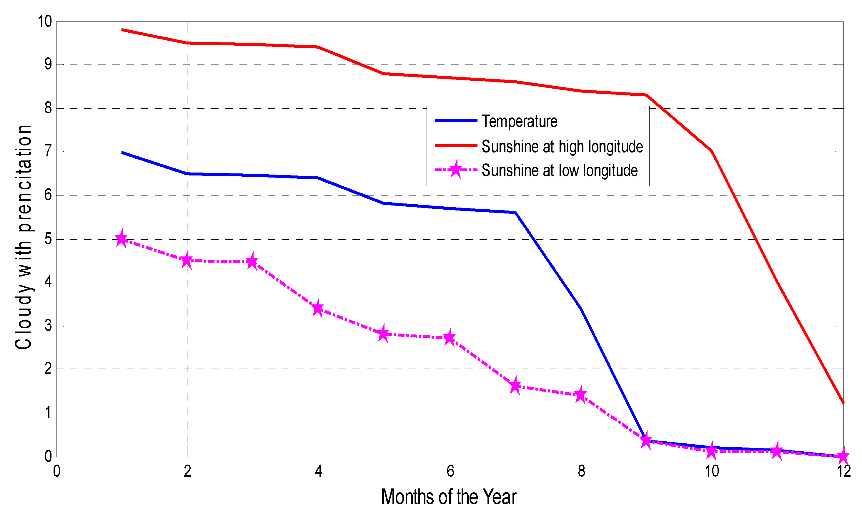
As the data observed from the Ethiopian meteorology institute shows that the sunshine value become rapidly decrease and become constant starting from the mid October to December.
3.4. Monthly Changeability of the Ionospheric Conductivity of Degem
Depending on the three models of geomagnetic ionospheric conductivity the hall model is rapidly increase at 00:00UT for the altitude variation from 10 to 300 Km and starting from the to it become slightily increase but starting from 200km it become very increase with constant value during January month and for 18:00UT of march month it become more increase starting from the altitude of 170km to 300Km.
Figure 5.
Ionospheric Conductance of the parallel, Pedersen and Hall conductivities on January and march of Degem.
Figure 5.
Ionospheric Conductance of the parallel, Pedersen and Hall conductivities on January and march of Degem.
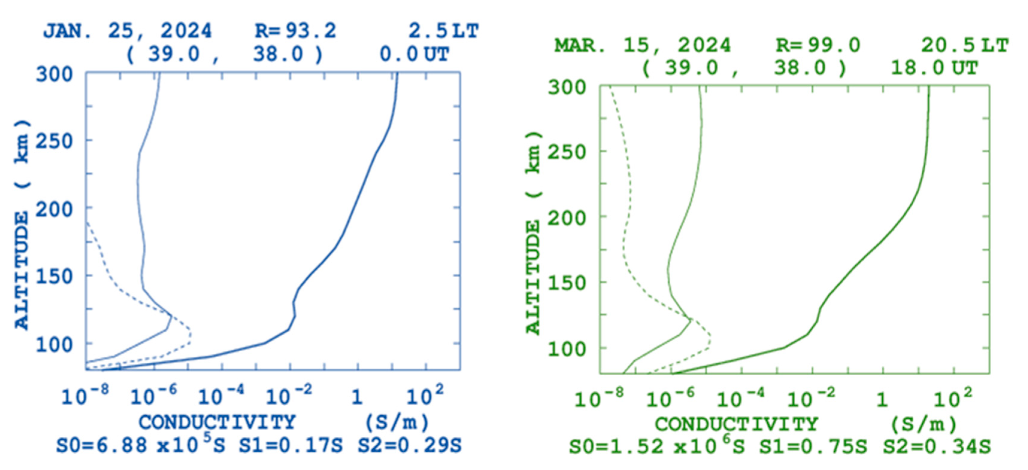
From the figure above the monthly changeability of the ionospheric conductivity is change of conductance from high solar activity to low solar conductivity, which mean by the ionospheric conductivity been reduced from day time to night time with the variation of 1440 minutes of a day. This ionospheric conductivity of the Degem is not the same within the same season the figure above shows that the daily variation is indicated in January and march 25 and 15 respectively at the 00: 00 and 18:00 UT for 2024. For both parallel and Pederson model the ionospheric conductivity, be come more increase at 00:00UT of January starting from and respectively. But for march 18:00UT, The parallel and the Pederson ionospheric conductivity more increase from 80km to 300km of altitude. From the January and march month the parallel ionospheric conductivity reaches and in respective.
3.5. Monthly Changeability of the Ionospheric Conductivity of Debre Libanos
The conductivity become increase in terms of the altitude starting from 150km to 300km and then become remain. Incase for March month of 03/2024 , it is increase up to the peak of 385km and reach the maximum ionospheric conductivity of .For parallel and Pederson model the ionospheric conductivity become increase with latitude variation and reach at the maximum conductivity .
Figure 6.
Ionospheric conductance of the parallel, Pedersen and Hall conductivities on January and march of Debre Libanos district.
Figure 6.
Ionospheric conductance of the parallel, Pedersen and Hall conductivities on January and march of Debre Libanos district.
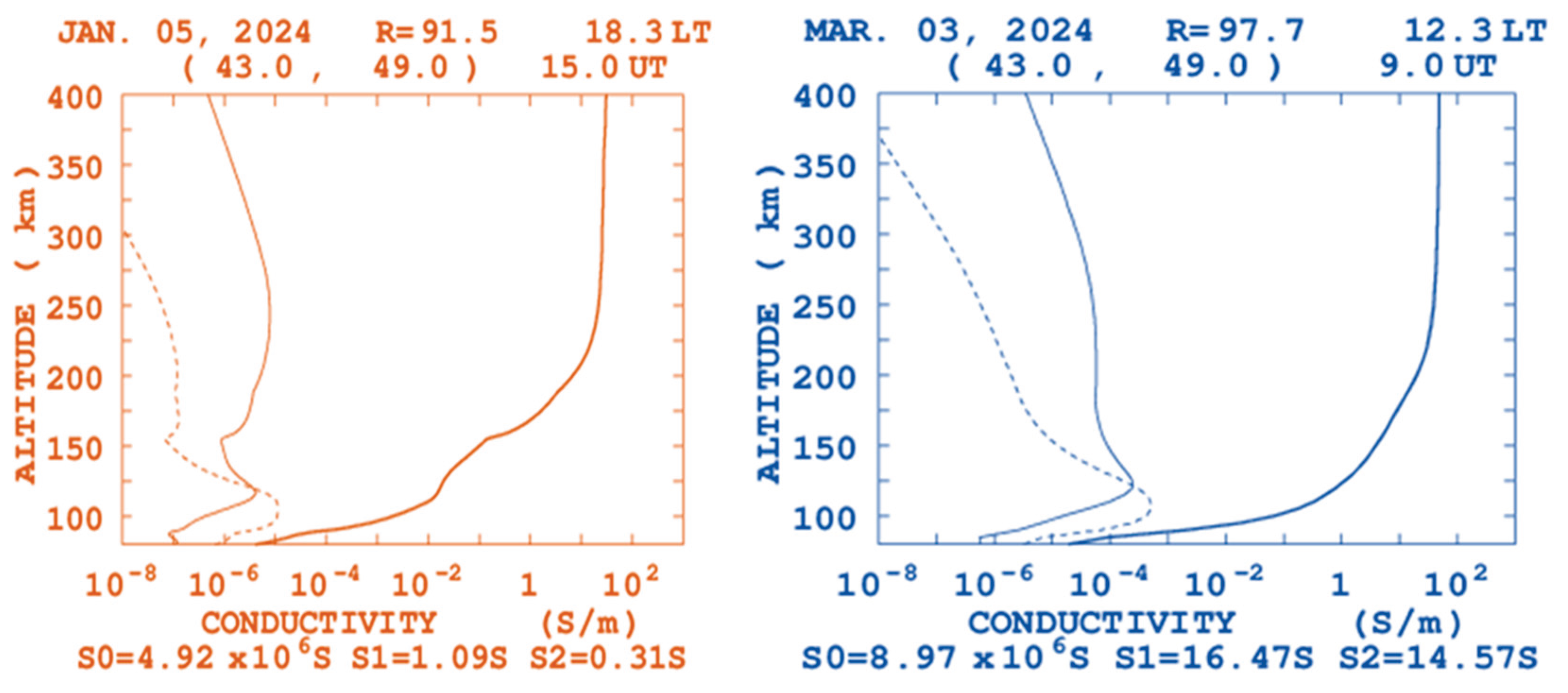
From the above figure due to the variation of longitude and latitude of the districts the ionospheric conductivity of hall, Pedersen and the parallel from left to right side the there is a variability for both months of January and march at a specific time of 15:00 UT and 9:00 UT. At 80Km of latitude of January month the hall ionospheric conductivity becomes slightly increase to and become decrease to .
4. Discussion
The ionospheric conductivity is primarily determined by the densities of local plasma's and their collisional frequencies with neutral molecules. Temperature and sunshine are parallel to each other in case at the sunshine is more active in ionosphere region. As the time rate run from morning to evening the life time of sunshine is increase rather than the life time of temperature. Which mean by the temperature value become decrease at evening than midday, at this time the ions are more movable in ionospheric regions. The space become clean and the ion transportation are freely transported in all dimensions. With the altitude increment the temperature become reduced; from this factor at a day time with short altitude the conductivity become evaluated freely. But during nighttime the plasma transport is an important for determination of conductivity at high altitudes to make coupling between the winds, plasma motion and plasma density.
The precipitation and cloud become takes place when the temperature value start to cool down from the maximum peak point to the minimum peak value; this is an evidence shown from the figure of monthly variation of cloud and sunshine with the factor of temperature variation. At the top of the altitude the temperature become decrease and it causes for the formation of cloud and precipitation. Even though during evening time around 6:47UT the sunshine is rayed at the top of some altitude and the ray of the sunshine is visible even the temperature is low for the current lines are aligned.
For both E and F region of ionosphere for the three ionospheric conductivity from Hall, Pedersen and Parallel conductivity, the ionospheric conductivity becomes varied. At nighttime ionospheric conductivity is distressed more than the daytime, but the daytime ionospheric conductivity become better than the nighttime. Comparing the value of conductivity from the graph of the three districts the day value of ionospheric conductivity is greater than at 00:00UT conductivity values. The three (Hall, Pedersen and Parallel) ionospheric conductivities become increase abruptly up to reach their peak values and again they keep the sharpness of their inconsistency after reaching the peal values. There is significant variability of the ionospheric conductivities are observed in each months; this is due to high solar activity disturbance of the daytime of solar activity in the high solar movement.
5. Conclusion
Interms of wave communication the energy is one of the most important factors for the frequency and for the latitude and longitude variability. As the plasma become collide with the neutrals ions and with winds. During the collision takes place the energy become loosed and the ionospheric particles start to keep remain at their original place change their direction of motion. This action was occurred during both night time and day time respectively. when the wave change direction the ions become disturbed and it need long wave length to reach at the origin, this causes the communication range become disturbed.
Author Contributions
Conceptualization: 1. and 6.; methodology, 1, 5 and 3.; software, 1. and 2.; validation, 2, 3, and 2.; formal analysis, 1. and 4.; investigation, 1. and 3.; resources, 7. and 1.; writing original draft preparation, 1, 2,3, 4 and 6.; writing—review and editing, 2,3,4 and 5.; supervision, 4 and 3. All authors have read and agreed to the published version of the manuscript.
Informed Consent Statement
Not applicable.
Data Availability Statement
The original contributions presented in this study and further inquiries can be directed to the corresponding author.
Conflicts of Interest
The authors declare no conflicts of interest.
References
- Brekke, A., Doupnik, J.R., Banks P.M. (1974), Incoherent scatter measurements of eregion conductivities and currents in the auroral zone, J. Geophys. Res., 79(25), 3773-3790.
- Cahill Jr. J. L. (1959). Investigation of the equatorial electrojet by rocket magnetometer. J. Geophys. Res. 64(5), 489-503. [CrossRef]
- Davis T, N., K. Burrows, J.D. Stolarik (1967), A latitude survey of the equatorial electrojet with rocket-borne magnetometers. J. Geophys. Res. 72, 1845-1861.
- Ebihara, Y., M.-C. Fok, R. A. Wolf, T. J. Immel, T. E. Moore (2004). Influence of ionosphere conductivity on the ring current. JOURNAL OF GEOPHYSICAL RESEARCH, VOL. 109, A08205. [CrossRef]
- Emmert, J. (2015). Thermospheric mass density: A review. Advances in Space Research, 56(5), 773-824. [CrossRef]
- Friis-Christensen, E. A. (1981). High latitude ionospheric currents. In Exploration of the Polar Upper Atmosphere (C. S. Deehr and J. A. Holtet, eds.). Reidel, Hingham, Massachusetts.
- Fuller-Rowell, T. J., Evans, D. S. (1987). Height-integrated Pedersen and Hall conductivity patterns inferred from the TIROS-NOAA satellite data. Journal of Geophysical Research, 92(A7), 7606-7618.
- Hardy, D. A., M. S. Gussenhoven, and E. Holeman (1985), A statistical model of auroral electron precipitation, J. Geophys. Res., 90, 4229.
- Heelis, R. A., Maute, A. (2020). Challenges to understanding the Earth's ionosphere and thermosphere. Journal of Geophysical Research: Space Physics, 125, e2019JA027497. [CrossRef]
- Jin, H., Miyoshi, Y., Fujiwara, H., Shinagawa, H., Terada, K., Terada, N., et al. (2011). Vertical connection from the tropospheric activities to the ionospheric longitudinal structure simulated by a new Earth's whole atmosphere-ionosphere coupled model. Journal of Geophysical Research, 116, A01316. [CrossRef]
- Liu, H., Thayer, J., Zhang, Y., Lee, W. K. (2017). The non-storm time corrugated upper thermosphere: What is beyond MSIS? Space Weather, 15, 746-760. [CrossRef]
- Maynard N. C. (1967). Measurements of ionospheric currents off the coast of Peru. J. Geophys. Res. 72(7), 1863-1875. [CrossRef]
- McGranagham, R., D. J. Knipp, T. Matsuo, H. Godinez, R. J. Redmon, S. C. Solomon, and S. K. Morley (2015). Modes of high-latitude auroral conductance variability derived from DMSP energetic electron precipitation observations: Empirical orthogonal function analysis, J. Geophys. Res. Space Physics, 120, 11,013-11,031. [CrossRef]
- McGranagham, R., D. J. Knipp, T. Matsuo, and E. Cousins (2016). Optimal interpolation analysis of high-latitude ionospheric Hall and Pedersen conductivities: Application to assimilative ionospheric electrodynamics reconstruction, J. Geophys. Res. Space Physics, 121, 4898-4923. [CrossRef]
- McPherron, R.L., Russell, C.T., Aubry, M.P. (1973). Satellite studies of magnetospheric substorms on August 15, 1968: 9. Phenomenological model for substorms. J. Geophys. Res. 78(16), 3131-3149. [CrossRef]
- Menk, F.W., D. Orr, M.A. Clilverd, A.J. Smith, C.L. Waters, D.K. Milling, and B.J. Fraser (1999). Monitoring spatial and temporal variations in the dayside plasmasphere using geomagnetic field line resonances, J. Geophys. Res., 104, 19955.
- Mikic, Z., Lee, M. A., (2006). An introduction to theory and models of CMEs, shocks and solar energetic particles. Space Science Reviews, 123, 57-80.
- Moen, J., A. Brekke (1993). On the importance of ion composition to conductivities in the auroral ionosphere, J. Geophys. Res.,95, 10,687-10. [CrossRef]
- Nagai, T., et al., (2003). Structure of the Hall current system in the vicinity of the magnetic reconnection site, J. Geophys. Res., 108, 1357.
- Pfaff Jr. R. F, M.H. Acuna, P.A. Marionni, N.B. Trivedi (1997). DC polarization electric field, current density, and plasma density measurements in the daytime equatorial electrojet. Geophys. Res. Lett. 24, 1667-1670.
- Prolss, G. W. (2011). Density perturbations in the upper atmosphere caused by the dissipation of solar wind energy. Surveys in Geophysics, 32(2), 101-195.
- Qian, L., Burns, A. G., Emery, B. A., Foster, B., Lu, G., Maute, A., et al. (2014). The NCAR TIE-GCM: A community model of the coupled thermosphere/ionosphere system. Modeling the Ionosphere-Thermosphere System, Geophysical Monograph Series, 201, 73-83.
- Qian, L., Solomon, S. C. (2012). Thermospheric density: An overview of temporal and spatial variations. Space Science Reviews, 168(1), 147-173. [CrossRef]
- Raeder, J., Wang, Y., Fuller-Rowell, T. J. (2001). Geomagnetic storm simulation with a coupled magnetosphere-ionosphere-thermosphere model. Washington DC American Geophysical Union Geophysical Monograph Series, 125, 377-384.
- Rasmussen, C. E., R. W. Schunk, and V. B. Wickwar (1988). A photochemical equilibrium model for ionospheric conductivity, J. Geophys. Res., 93(A9), 9831-9840.
- Richmond A. D. (1979). Ionospheric Wind Dynamo Theory: A Review, J. Geomag. Geoelectr., 31, 287-310.
- Richmond A. D. (1989). Modeling the ionosphere wind dynamo: a review. quiet daily geomagnetic fields. Pure Appl. Geophys. 131, 413-435.
Disclaimer/Publisher’s Note: The statements, opinions and data contained in all publications are solely those of the individual author(s) and contributor(s) and not of MDPI and/or the editor(s). MDPI and/or the editor(s) disclaim responsibility for any injury to people or property resulting from any ideas, methods, instructions or products referred to in the content. |
© 2025 by the authors. Licensee MDPI, Basel, Switzerland. This article is an open access article distributed under the terms and conditions of the Creative Commons Attribution (CC BY) license (http://creativecommons.org/licenses/by/4.0/).
Copyright: This open access article is published under a Creative Commons CC BY 4.0 license, which permit the free download, distribution, and reuse, provided that the author and preprint are cited in any reuse.


