
Submitted:
23 December 2025
Posted:
24 December 2025
You are already at the latest version
Abstract
This study presents a robust constitutive model for clays capable of capturing mechanical behavior over a wide range of plasticity and overconsolidation ratios (OCR). The model is formulated within a bounding-surface plasticity framework and employs a teardrop-shaped yield surface controlled by two shape parameters, Ψ and Ω, which regulate yield-surface skewness and shear strength, respectively. An explicit plastic potential is introduced to eliminate the stress–dilatancy paradox and to obtain a linear, physically interpretable stress–dilatancy relation. Model parameters are calibrated using conventional laboratory data and are linked to standard oedometer indices, preserving practical applicability. Validation against triaxial test results for clays with contrasting plasticity demonstrates that the model consistently reproduces both curved and nearly linear stress paths at low stress ratios, as well as a smooth transition from normally consolidated to overconsolidated behavior. The proposed formulation provides a unified and robust framework suitable for numerical implementation and geotechnical engineering applications.
Keywords:
bounding surface
; constitutive model
; high-plasticity clay
; low-plasticity clay
; low stress ratios
; over consolidated clay
; normally consolidated clay
1. Introduction
In practical geotechnical engineering, clay deposits rarely consist of a homogeneous material with a uniform overconsolidation ratio (OCR). Instead, they often contain strata exhibiting variations in OCR [1,2,3,4,5,6,7,8]. Consequently, geotechnical analyses should adopt a robust constitutive model capable to rigorously predicts the mechanical response of both normally consolidated (NC) and overconsolidated (OC) clays over a wide range of OCRs formulated within a unified theoretical framework.
The original Cam Clay (OCC) [9] and Modified Cam Clay (MCC) [10] models were the first two elastoplastic constitutive models originally developed to describe the behavior of normally consolidated (NC) clays within the framework of Critical State Soil Mechanics (CSSM). It is evident that, in subsequent studies, numerous modifications of the MCC model have been proposed to improve its applicability to geomaterials (e.g., [11,12,13,14,15,16,17,18,19,20,21,22]). For overconsolidated (OC) clays, the yield function (f) of the MCC model—characterized by its elliptical shape—tends to overestimate the peak strength of heavily overconsolidated materials on the dry side of the critical state [23,24,25,26,27]. Therefore, the dry side portion of the MCC yield surface is commonly revised to better capture the OC behavior. A key feature in such reformulations is the incorporation of the Hvorslev envelope [28] into the yield function, resulting in the familiar bullet- or teardrop-shaped yield surfaces. Embedding the Hvorslev envelope in the MCC yield function enhances peak-strength predictions for moderately to heavily overconsolidated clays while maintaining a smooth surface-gradient transition across all stress ratios.
On the wet side of the bullet/teardrop yield surface, the formulation generally remains similar to the Modified Cam Clay (MCC) model. This portion of the surface provides a convex stress path for normally consolidated (NC) clay (as illustrated in Figure 1a–b) and performs well for clays that exhibit relatively low plastic deformation under low stress ratios, = q/p (hereafter referred to as LPLS). In Figure 1 and the related text, the mean effective stress p and deviatoric stress q are defined following the fundamental principle of soil mechanics as p = ()/3 and q = where , and are the principal stresses satisfying . The parameter denotes the preconsolidation pressure, representing the maximum historical mean effective stress that controls the current yield and bounding surfaces. The Critical State Line (CSL), defined by , marks the ultimate stress condition where plastic volumetric strain ceases. The normalized form was used to remove dimensional influence and enable direct comparison among clays with different consolidation histories. This normalization also highlights the relative position of the current stress state with respect to its yield surface, thus facilitating a unified interpretation for both normally and overconsolidated clays.
However, certain clays deviate from this behavior: while the models may predict responses reasonably well for overconsolidated (OC) clays with OCR > 1, they often fail to reproduce NC behavior with comparable fidelity. This limitation diminishes their practical applicability in geotechnical analysis, as inadequate representation of even a single clay stratum can compromise the reliability of the overall boundary-value solution. Such clays frequently follow nearly linear stress paths in the p–q plane, rather than the curved trajectories shown in Figure 1c–d, reflecting the onset of substantial plastic straining from the very early stages of loading—even under low stress ratios (denoted as HPLS in this study).
In addition, in modeling normally consolidated (NC) clay, it is generally assumed that no plastic strain develops inside the yield surface. However, for overconsolidated (OC) clays, plastic strains may occur even within the yield surface. To capture this behavior, a bounding surface plasticity framework was introduced for OC clays (e.g., 29-30,32-33) with the adaptation of a non-associated flow rule, in which the yield function differs from the plastic potential function . Although the exact form of g is not explicitly known, it can be evaluated based on the principle of stress–dilatancy D, defined as the ratio of plastic volumetric strain to plastic deviatoric strain, given by . It should be noted that, when applying D in constitutive formulations, a paradox arises because is often assumed to equal instead of (e.g., [29,30,32]). Therefore, to eliminate this paradox in models employing the bounding surface plasticity framework, an appropriate specification of the plastic potential function g is required.
The primary objective of this study Is to develop a unified constitutive model capable of capturing the behavior of both normally consolidated (NC) and overconsolidated (OC) clays, with particular emphasis on NC clays that exhibit both low- and high-plastic deformation under low stress ratios. To achieve this objective, several new theoretical features are introduced. First, a dual-parameter control (, ) is embedded into the yield function to enable flexible and explicit regulation of the yield-surface skewness and curvature. Second, an explicitly defined plastic potential function is formulated to eliminate the long-standing stress–dilatancy paradox in bounding-surface-type models. Third, a linear stress–dilatancy relation is adopted to ensure physical transparency and facilitate practical parameter calibration. Through these features, the proposed formulation provides a unified framework that can consistently capture both LPLS and HPLS responses within a single constitutive structure, thereby advancing the state of the art in constitutive modeling of clays under low stress ratios.
2. Formulations of the Constitutive Model
2.1. Yield and Plastic Potential Functions
In this section, for the sake of clarity, we begin with the plastic potential function g, followed by the yield function f, noting that certain elements of the latter have evolved from the former. We then proceed to examine appropriate pairs of plastic-potential and yield functions that enable the model to reproduce the behavior of both low- and high-plasticity clays under a consistent and compatible f-g formulation.
2.1.1. Plastic Potential Function
As noted earlier, the explicit form of the plastic potential function g is generally unknown. However, the use of the stress–dilatancy relation D within the bounding-surface plasticity framework provides a practical relationship that is easier to determine experimentally, albeit unavoidably accompanied by a well-known paradox. In this study, we establish an explicit form of g. Inspired by the work in [33], which proposed a model applicable to both NC and OC clays and presented the plastic potential surface as a left-skewed teardrop without a closed-form equation, we adopt the closed-form expression of the original Cam-Clay (OCC) yield function [9] as the plastic potential function g. This formulation yields a left-skewed teardrop surface similar to that in [33], as given in Equation 1. The resemblance in shape provides an appropriate gradient for computations within the bounding-surface plasticity framework, and having an explicit form of g completely eliminates the paradox inherent in the theory. Consequently, the plastic potential surface g used in this study can be directly compared in size and shape with the elliptical yield surface of MCC, as illustrated in Figure 2.
2.1.2. Yield Function
Once, the Modified Cam Clay (MCC) model [10] was developed by improving the yield function of the original Cam Clay (OCC) model [9]. This modification was motivated by the observation that the OCC yield function did not fully reproduce the experimental behavior of normally consolidated (NC) clays, whose yield surface on the wet side should be nearly vertical to the p-axis at the point (the low-stress-ratio region). Such behavior corresponds to the LPLS condition discussed earlier in this study.
However, later literature clearly reported that some NC clays do not exhibit this LPLS-type response; instead, their stress paths are inclined linearly, consistent with the yield function of the OCC model—referred to here as HPLS-type. It is therefore evident that neither the OCC nor the MCC model can fully capture the mechanical behavior of both clay types within a single constitutive framework. Accordingly, an appropriate yield function should be capable of representing both responses within one unified model. This consideration provides the fundamental motivation for developing a new unified yield function in the present study.
In constructing this unified function, the OCC yield function was adopted as the baseline because it already reproduces the HPLS-type response satisfactorily. Further modifications were then introduced so that the model could also describe the LPLS-type behavior.
The OCC yield function inherently exhibits a left-skewed shape. To enable the model to also represent the right-skewed form associated with the LPLS condition, the yield-surface shape must be controlled through a suitable parameter, here denoted as , introduced in the term of the OCC yield function. Figure 3a illustrates the influence of on the yield surface shape, showing its transition from left- to right-skewed forms for values of = 1 to 3. Specifically, = 1 represents a left-skewed shape, = 2 corresponds to a right-skewed one, and intermediate values (1 < < 2) capture transitional clay behavior between these two extremes.
Additionally, cases with > 2, also included in Figure 3a, allow the model to reproduce clay behavior exhibiting high-strain softening or a distinct stress-path peak. Furthermore, it is essential to accurately control the shear strength at the critical state ( = M), corresponding to the intersection of the yield function with the Critical State Line (CSL) (e.g., [27]). Therefore, another parameter, denoted as , was introduced in the term of the OCC yield function to precisely govern this critical-state shear strength. The corresponding equation is presented in Equation 2.
Accordingly, Equation 2 is formulated as a revised Cam-clay-type yield function, expanded into a general logarithmic form with two shape parameters ( and ). These parameters provide flexible control of both the wet- and dry-side curvature, enabling the surface to reproduce right- or left-skewed teardrop shapes. The conceptual basis was inspired by Hvorslev-envelope-based yield functions (e.g., Yao et al., 2009; Chen & Yang, 2017) but re-parameterized here to achieve symmetric and continuous curvature control.
It is worth noting before proceeding that the physical meaning of lies in controlling the skewness of the teardrop-shaped yield function, whereas serves as a shear-strength adjuster across different OCRs. These interpretations provide a convenient basis for subsequent referencing throughout this study and for establishing practical guidelines for selecting these two parameters.
A general form of the yield function, once plastic strain develops beyond zero after loading has commenced, incorporates a hardening parameter H, which is defined as a function of plastic strain as follows:
and
where , is the initial void ratio, denote the slope of virgin compression line (VLC) and unloading-reloading line in the one-dimensional Oedometer test, respectively.
Figure 3b presents the model predictions obtained in this study using the plastic potential function g in Equation 1 together with the yield function f in Equation 2. The figure illustrates how variations in the state parameter lead to distinct degrees of curvature or straightness in the stress paths for NC clays. These variations in provide a preliminary indication that an appropriate and feasible pair of f and g can accommodate both HPLS and LPLS behaviors within a single yield function.
In the proposed model, the yield function f and the plastic potential function g are formulated to operate in tandem, thereby enhancing the predictive capability for both normally consolidated (NC) and overconsolidated (OC) clays, encompassing low- and high-plasticity soils under low stress ratios. The framework can be categorized into two representative forms, as illustrated in Figure 4. In Figure 4a, f exhibits a right-skewed curve while g adopts a left-skewed curve, a combination that is particularly suited to modeling low-plasticity clays under low stress ratios (LPLS). Conversely, Figure 4b presents a pair of left-skewed surfaces for both f and g, which proves more appropriate for capturing the behavior of high-plasticity clays at low stress levels (HPLS).
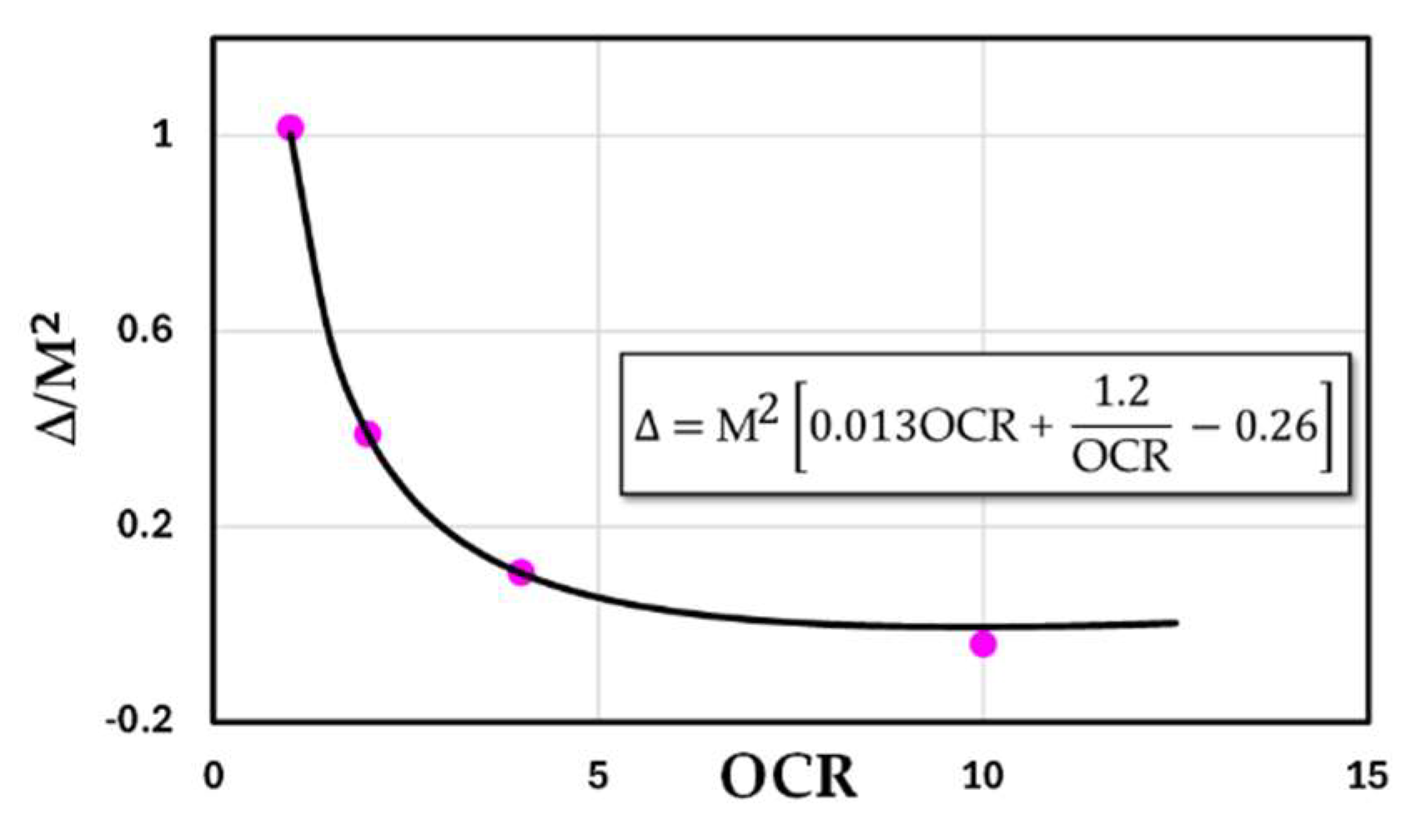
A general guideline for selecting the shape parameters and can be established by linking their roles to conventional clay indices obtained from one-dimensional oedometer tests. For NC clays exhibiting markedly curved p′–q stress paths, ≈ 1.2–1.4 with = 1.0 is recommended, whereas nearly linear responses can be reproduced using = = 1.0. Additional refinement can be achieved by adjusting slightly above or below unity to increase or decrease the predicted shear strength. Consistently, the calibrated values in Table 1 remain close to one (0.93–1.17), providing a practical starting range.
Further analyses show the practical guideline that and correlate strongly with (), where and represent the slopes of the virgin compression line and the unloading–reloading line, respectively, in the e–ln(p) plane obtained from oedometer tests as shown in Figure 5. These empirical relationships (Equations 5–6) provide an objective basis for parameter estimation and enhance the reproducibility of the model.
2.2. Dilatancy Equation
An important advantage of employing stress–dilatancy D is that it enables the simulation of both volumetric () and deviatoric ) plastic strain increments, even when the plastic potential function g is not explicitly defined. In the classical bounding-surface plasticity framework, the plastic potential function is often not readily available in closed form. Accordingly, the stress–dilatancy relation—defined as the ratio of the volumetric to the deviatoric plastic strain increments—has been widely adopted in the literature, as it can be more straightforwardly identified from experimental observations. This ratio, referred to as stress–dilatancy, is expressed as shown in Equation 7.
From the theory of plasticity, the plastic strain increments are computed as the product of a proportionality constant and the gradient of the plastic potential function g, such that and . As a result, the stress–dilatancy ratio becomes independent of the plastic multiplier , and can be written directly in terms of the gradients of g, leading to the following expression:
For OC clays, the most widely adopted expression of D is the second-order dilatancy formulation of the Modified Cam-Clay (MCC) type (e.g., [29,34,35,36]). Although higher-order stress–dilatancy relations have also been proposed to capture the behavior of both normally consolidated (NC) and OC clays [30,32], closer examination reveals that, for stress ratios η not exceeding the critical state stress ratio M (approximately 1.3–1.4), a first-order or linear dilatancy relation provides satisfactory predictions and yields results comparable to the second-order formulation. Moreover, as highlighted in [30], although a high-order dilatancy expression was proposed, the parameter values adopted in practice often reduce the equation to, or make it nearly equivalent to, a linear approximation. This observation is supported by Figure 6, which presents the relationship between D and η for Fujinomori Clay and Lower Cromer till. The results confirm that, within the practical range of , a linear approximation D- remains appropriate. In addition, opting for such a simplified linear form facilitates practical implementation while maintaining predictive adequacy.
In the proposed model, an explicit expression for g is formulated, as shown in Equation 1, thereby eliminating the paradox entirely. The expressions for and can be derived as presented in Equations 8–9.
Substituting Equation 8 and Equation 9 into Equation 7 yields:
It is evident that the expression for D in Equation 10 is linear, which is consistent with the experimental data for Fujinomori clay [37] and Lower Cromer till [38] presented in Figure 6. This confirms that the explicit derivation of the plastic potential function in this study leads to a physically consistent stress–dilatancy response observed in experiments. Accordingly, the plastic potential function is shown to be in agreement with the experimental results without introducing any paradox within the model. A limitation of the linear stress–dilatancy formulation adopted in Equation 10 is that, as shown in Figure 6, each experimental D– curve exhibits a practical upper limit. For the clays examined in this study, the stress ratio remains within this range, and the linear approximation is therefore appropriate. If stress ratios approach such limits in practice, higher-order dilatancy relations may be required; however, these generally preclude an explicit plastic potential function and may reintroduce the stress–dilatancy paradox.
2.3. Bounding Surface
Once the yield surface has been properly defined, the bounding surface can be established by employing the principle of a smooth transition from the OC state to the NC state. Hence, the shape of the bounding surface is identical to that of the yield surface defined in Equation 2. The bounding surface employed in this model is expressed as follow:
where is the model parameter controlling the shape of the bounding surface. The distinctive feature of this formulation is that the bounding surface can take a left-skewed form ( = 1) or a right-skewed form ( = 2). In general, = 1.0 is appropriate for soils whose stress paths for NC clay on the p–q plane is nearly linear, corresponding to high plastic deformation under low stress ratios (HPLS). By contrast, values of in the range of approximately 1.2–1.4 are suitable for soils exhibiting low plastic deformation under low stress ratios (LPLS). The equations required for elastoplastic computations , and are presented in Equations 12-14, respectively.
Another fundamental aspect in modeling overconsolidated (OC) clays is the application of the mapping rule. In general, when clay initially resides in an OC state, the increasing applied load causes its stress state to gradually transition toward an NC-like condition, depending on the magnitude of loading and the soil’s stress history [31]. The mapping rule establishes a correspondence between the stress state at the current stress point—commonly referred to as the loading surface—and the stress state defined on the bounding surface. This linkage facilitates a smooth mechanical transition from the OC state to the normally consolidated (NC) state through the spacing ratio , as illustrated in Figure 7. When , the stress point lies inside the bounding surface and plastic strains are gradually mobilized through the mapping mechanism, enabling progressive yielding in OC clays. As , the stress state approaches the bounding surface and the response naturally converges to the NC behavior governed by the hardening law. Typically, both surfaces are assumed to share a similar shape, with the current loading surface being smaller in size and nested within the bounding surface. In practical terms, the spacing ratio controls the degree of plasticity, stiffness degradation, and peak strength development, which is particularly important for soils exhibiting complex stress–strain behavior.
2.4. Hardening Law and Plastic Modulus
Although, for the OC state, the stress of clay lies on a portion of the unloading–reloading line on e-ln(p) plane with a slope equal to κ, where conventional calculations give only purely elastic strains though a constant However, in the bounding surface plasticity framework, it is common to introduce an alternative approach to enable OC clays to develop plastic strains in addition to elastic strains. Specifically, it assumes that the stress point lies on the isotropic compression line which has a slope of . This conceptual framework not only allows the model to capture plastic strains in OC clays but also provides a rational basis for employing the parameter in the hardening law. Accordingly, the isotropic hardening law can be consistently applied to both the NC and OC states within a unified framework. The hardening law employed in this model is expressed as follows:
where is the volumetric plastic strain increment. From Equation 15, for a single sub-step computation, can be determined as For the plastic modulus which is employed together with the proportional constant to determine the change of the hardening parameter in consistency condition which expressed as . By substituting this relation into Equation 3 and rearranging, the expression for can be obtained as presented in Equation 16.
Upon closer examination Equation 16, using stress point (P, Q) is highly restricted to OCR = 1, because P and Q are located on the bounding surface. To allow valid for OCR > 1—i.e., for stress states on the loading surface that is nested within the bounding surface—it is therefore necessary to revise so it remains applicable to both normally and overconsolidated clays.
A key mechanism enabling plastic strain for stress points located inside the bounding surface via is that must be a positive number at the critical state. However, as given by Equation 16, vanishes at the critical state which is a condition appropriate for normally consolidated clay but unsuitable for overconsolidated clay. To address this, Dafalias and Herrmann (1986) [39] proposed the concept of a virtual peak stress ratio, , to replace M in Equation 16, thereby providing a smoother and more accurate description of OC behavior. The expression for is shown in Equation 17.
where M is the stress ratio at the critical state, R is the spacing ratio, and n is a positive parameter. Since the spacing ratio R equals 1 when the stress state lies on the bounding surface, becomes identical to M, but takes values greater than M when the stress point lies inside the bounding surface. Consequently, for cases with OCR > 1, the stress–strain response may exhibit a peak at a stress ratio exceeding M.
The parameter n in Equation 17 is introduced to adjust the virtual stress ratio , and consequently the plastic modulus . When OCR = 1, the parameter n has no effect because the spacing ratio R equals unity. Although many models employ a constant value for n. However, for OCR > 1, a value of n should lead to a different value of both and . Intuitively, this suggests that n may not be a constant but rather a quantity related to the soil’s overconsolidation history, since its influence on model responses varies with OCR. In [29] a power-law regression for n-OCR has been proposed. Nevertheless, this equation may be compatible only with specific constitutive models, depending on the mapping rule adopted. In this study, a new n–OCR relationship is proposed as presented in Equation 18.
Another crucial issue in considering the parameter n is whether it should take the same value for both undrained and drained loading conditions. It is well known that the drained shear strength is generally higher than the undrained shear strength due to the pore pressure that develops during undrained loading. However, the difference between drained and undrained shear strength () decreases with increasing OCR. Figure 8 depicts the typical paired stress paths for drained and undrained conditions across various OCR values, clearly demonstrating that the shear strength difference is OCR-dependent. Moreover, Figure 8 also reveals that the critical state stress ratio M exerts an additional influence on ; specifically, larger values of M correspond to greater values of . Hence, the relationship can be expressed as = f(OCR, M).
In this study, the relationship among , OCR, and M is presented in Figure 4 and expressed in Equation 19. From Equation 19, it can be observed that is more precisely defined as = f(OCR, ). Accordingly, it may be inferred that the parameter plays a key role in differentiating the value of n between drained and undrained cases. The specific expression for n under drained loading is provided in Equation 20.
Figure 9.
Comparison of the disparity between drained and undrained shear strengths at the critical state for various OCR values.
Figure 9.
Comparison of the disparity between drained and undrained shear strengths at the critical state for various OCR values.
3. Elastoplastic Constitutive Relations
The constitutive models employing the stress p and q implicitly adopt the Extended Mises failure criterion, which forms a circular failure envelope on the -plane and typically leads to an overestimation of shear strength. This limitation can be eliminated by employing the SMP failure criterion [13] as shown in Figure 10. The present model also adopts this approach by employing a transformed stress formulation to integrate the SMP criterion to the proposed model. A brief description of the transformed stress and the SMP criterion is provided prior to presenting the governing equations of the proposed model.
3.1. Transformed Stress Tensor
A transformed stress tensor is employed instead of the ordinary stress tensor in the analyses to improve shear strength prediction by introducing the SMP criterion [13]. Once the is given, the can be calculated as follows:
where is the Kronecker’s delta, and are the mean stress and deviatoric stress tensor calculated from the ordinary stress tensor, respectively, and are the mean stress and deviatoric stress tensor calculated from the transformed stress tensor, respectively, which can be written as
and are the radius of the circular cone and the Extended Mises cone which can be calculated using
where , and are the first, second, and third stress invariants, respectively.
3.2. Stress–Strain Modelling for Elastoplastic Constitutive Model
The total strain increment is decomposed into elastic and plastic components as follows:
In the calculation of , it can be computed by applying the consistency condition (dF = 0) conjunction with application of chain rule, as shown in Equation 27.
Thus,
It is worth noting that in Equation 28 is highly beneficial for conducting drained analyses, since the pore pressure is zero and the input data can therefore be directly expressed in terms of the stress increments dP and dQ. In contrast, for undrained analyses, the input for the computation (especially in the numerical analyses) must be given in terms of strain increments with the condition of . The corresponding calculations can then be carried out as follows.
Where
and the elastic bulk and shear modulus can be expressed in term of the initial void ratio , the Poisson’s ratio and the slope of unloading-reloading line in e-ln(p) plane ( as
The elastic and plastic strain increment can be written as follows:
thus,
where h() = 1 for > 0, and h() = 0 when < 0. The stress-strain relationship can be calculated as
Before presenting a comparison between the analytical results of the proposed model and the experimental data in the following section, the final part of this section illustrates the variation of the model’s predictions, with particular emphasis on the influence of the parameter . This parameter constitutes a key factor enabling the model to reproduce clay behavior as either HPLS or LPLS across different OCR values. Figure 11 depicts the normalized stress paths (p′/ – q/) for OCR values of 1, 2, 6, and 20 conjunctions with in the range of 1.0–3.0. It can be observed that Ψ effectively captures the characteristic responses of HPLS and LPLS for normally consolidated clays (OCR = 1) as well as for slightly to moderately overconsolidated clays (OCR ≈ 2). However, in the case of heavily overconsolidated clays, the results converge, showing little distinction across different values. This outcome is consistent with the aforementioned aim of this study.
4. Model Verifications and Discussions
In this section, the results obtained from the proposed model are presented for both drained and undrained analyses. The results are compared against experimental data for four clays i.e., Boston Blue clay (OCR = 1, 2, 4 and 8), Lower Cromer till (OCR = 1, 2, 4 and 10), Kaolin clay (OCR = 1, 1.2, 1.45, 1.8, 2.5, 3, 4.5 and 6.5) and London clay (OCR = 1, 2, 6 and 20). Furthermore, for each of these clays, the experimental results are systematically compared with predictions from three constitutive models: (I) the proposed model, (II) the model introduced by Xu et al., 2024 [30], and (III) the model developed by Chen and Yang, 2017 [29]. The soil parameters used in the analyses for 3 models mentioned above are summarized in Table 1.
To ensure the reliability of the proposed formulation, model validation was performed against well-documented triaxial test data under both drained and undrained compression and extension conditions. Because any constitutive model represents the stress–strain behavior of soil, it is rational to assess its accuracy through characteristic stress paths (e.g., or normalized ) and strain-based relationships such as and , where , , and denote the axial, volumetric, and deviatoric strains, respectively. All these quantities are typically obtained from triaxial compression and extension tests, and the corresponding comparisons between calculated and experimental results are presented in Figure 12, Figure 13, Figure 14, Figure 15, Figure 16, Figure 17, Figure 18, Figure 19 and Figure 20.
4.1. Undrained Analysis
Figure 12, Figure 13, Figure 14 and Figure 15 present comparisons between the triaxial compression test results and the predictions of the three aforementioned models, shown separately for each model to highlight their differences. In particular, the proposed model demonstrates superior capability in modeling the high plasticity under low stress ratio (HPLS) behavior compared with the other models. The corresponding comparison for the undrained triaxial extension test is provided in Figure 16 and Figure 17.
It is clearly evident from the triaxial compression test results of London clay and Lower Cromer Till, shown in Figure 12 and Figure 13, respectively. Both London clay and Lower Cromer till can be classified as exhibiting high plasticity under low stress levels (HPLS), as the stress paths for OCR = 1 display a pronounced inclination from the very onset of loading—a characteristic not commonly observed. Nevertheless, the proposed model provides predictions that align closely with the experimental results. By contrast, in both figures, the other two models of Xu et al. (2024) and Chen and Yang (2017) fail to capture this behavior adequately. Their predicted stress paths instead correspond to low plasticity under low stress levels (LPLS). In addition, it is observed that for both soils, all the models yield comparable predictions when OCR > 2.
For the experimental results of Boston Blue Clay and Kaolin Clay, shown in Figure 14 and Figure 15, respectively, the stress paths at OCR = 1 exhibit a pronounced curvature consistent with the bullet/teardrop-shaped yield surface in bounding surface models. This behavior is characteristic of clays classified as having low plasticity under low stress ratios (LPLS). In both figures, all three models successfully reproduce stress paths consistent with LPLS behavior. Among them, the proposed model and the model of Xu et al. 2024) demonstrate relatively high accuracy across all OCR values, whereas the model developed by Chen and Yang (2017) provides reasonable accuracy only for OCR > 1, while at OCR = 1 it tends to overestimate the response.
The ability of the proposed model to reproduce both the nearly linear HPLS-type and the curved LPLS-type stress paths directly reflects the combined roles of the yield surface parameter Ψ and the plastic potential function g introduced in Section 2.1, as illustrated earlier in Figure 2, Figure 3 and Figure 4.
For the undrained triaxial extension tests on Lower Cromer Till shown in Figure 16, the simulated stress paths are in good agreement with the experimental results, and the model also reproduces shear strengths comparable to the tests at OCR = 1, 2, 4, and 10. This is attributed to the use of the SMP failure criterion, which accurately captures the shear strength envelope, thereby reflecting the well-known fact that the undrained triaxial extension shear strength is lower than that under undrained triaxial compression. It should be noted that Lower Cromer till under undrained loading exhibits high-plasticity behavior at low stress ratios (HPLS) in both compression and extension, underscoring the existence of clays that truly fall into the HPLS category. By contrast, for the undrained triaxial extension tests on Kaolin clay (Figure 17), the stress path exhibits low-plasticity behavior at low stress ratios (LPLS). In this case, the model underestimates the shear strength at OCR = 1 and 1.2 but provides close agreement with the experimental data at OCR = 6 and 10.
4.2. Drained Analysis
To further evaluate the predictive capability of the proposed model, three drained triaxial compression test results were selected for comparison. In addition to the Lower Cromer till, the parameters and test results of two other clays—Shanghai clay and Fujinomori clay—were also considered in the investigation, as summarized in Table 2. Figure 18, Figure 19 and Figure 20 present the test results and corresponding model predictions for Lower Cromer till (OCR = 1, 1.25, 1.5, 2.0, 4.0, and 10), Fujinomori clay (OCR = 1, 2, 4, and 8), and Shanghai clay (OCR = 1, 2, 4, 8, and 12).
The comparisons in Figure 18, Figure 19 and Figure 20 show a close agreement between the experimental data and model predictions. For Lower Cromer till, the normalized stress–strain curves reveal contractive behavior at OCR = 1–4, characterized by curved stress paths without a distinct peak, along with residual shear strengths that vary systematically with OCR. In contrast, Shanghai clay exhibits contractive behavior without a peak at OCR = 1–4, but transitions to a contractive response followed by dilation at OCR = 8 and 10. Notably, for all OCR values, Shanghai clay develops essentially the same residual shear strength. Fujinomori clay demonstrates responses similar to Shanghai clay: contractive behavior without a peak at OCR = 1–4, followed by contractive behavior and subsequent dilation at OCR = 8, with residual shear strength remaining nearly constant across all OCR values. The proposed model successfully captures this behavior in close agreement with the experimental results.
From a practical geotechnical engineering perspective, the proposed model can be readily implemented in numerical analyses for problems involving soft to stiff clays under low stress ratios, such as shallow foundations, staged embankment construction, and consolidation-induced shear. The unified description of both normally consolidated and overconsolidated behaviors within a single framework allows engineers to simulate loading–unloading–reloading processes without switching constitutive models. In particular, the ability to reproduce both high- and low-plasticity clay responses provides a practical advantage for site conditions where clay plasticity varies spatially. These features make the model suitable for predicting stress–strain and volumetric responses in complex field conditions while maintaining a relatively simple parameter calibration procedure.
5. Conclusions
This study presents a unified bounding-surface plasticity formulation that reproduces both high-plasticity (HPLS) and low-plasticity (LPLS) clay responses under low stress ratios across a broad OCR range. The model combines a teardrop-shaped yield surface controlled by the shape parameters and , an explicit plastic-potential that resolves the dilatancy paradox, a practical linear stress–dilatancy relation , and an OCR-sensitive virtual peak ratio. Together, these ingredients produce a coherent, implementation-friendly framework with smooth NC↔OC transitions and no ad-hoc model switching.
Although two additional shape parameters are introduced, they can be directly determined from standard clay indices ( and ), preserving the parameter parsimony typical of MCC while enhancing predictive capability. Validation against undrained and drained tests shows that the model captures the steep, near-linear NC paths characteristic of HPLS clays and the curved trajectories of LPLS clays, as well as correct contractive behavior at low OCR and contractive-to-dilative transitions at higher OCR—without inflating the parameter set or requiring higher-order dilatancy forms.
From an engineering perspective, the formulation offers a single, interpretable constitutive model that is straightforward to calibrate from standard triaxial and oedometer data, preserves numerical robustness, and is readily implementable in finite-element analyses for practical geotechnical design, enabling consistent prediction of clay behavior under coupled loading, unloading, and consolidation processes within a unified constitutive framework.
Author Contributions
Conceptualization, T.C. and N.K.; methodology, T.C., N.P. and N.K.; software, T.C. and N.K.; validation, T.C., N.K. and A.K.; formal analysis, T.C. and N.K.; investigation, T.C. and N.P.; resources, T.C., S.I. and N.P.; data curation, T.C., N.P. S.I. and N.K.; writing—original draft preparation, T.C., N.K., S.K., N.P. A.K. and S.S.; writing—review and editing, T.C., N.K., S.K., A.K. and S.S.; visualization, S.K., S.I. and S.S.; supervision, N.K., S.K. and A.K.; project administration, T.C., S.I. and S.S.; funding acquisition, N.K. All authors have read and agreed to the published version of the manuscript.
Funding
This research was funded by Mahasarakham University.
Data Availability Statement
The original contributions presented in this study are included in the article. Further inquiries can be directed to the corresponding author.
Acknowledgments
This research was supported by Mahasarakham University. The support is gratefully acknowledged.
Conflicts of Interest
The authors confirm that they are no conflict of interest with respect to the publication of this paper.
References
- Bo, M.W.; Arulrajah, A.; Sukmak, P.; Horpibulsuk, S. Mineralogy and geotechnical properties of Singapore marine clay at Changi. Soils Found. 2015, 55, 600–613. [Google Scholar] [CrossRef]
- Bo, M.W.; Arulrajah, A.; Leong, M.; Horpibulsuk, S.; Disfani, M.M. Evaluating the in-situ hydraulic conductivity of soft soil under land reclamation fills with the BAT Eng. Geol. 2014, 168, 98–103. [Google Scholar]
- He, P.; Newson, T. Undrained capacity of circular shallow foundations on two-layer clays under combined VHMT loading. Wind Eng 2023, 46, 579–96. [Google Scholar] [CrossRef]
- DeGroot, D.J.; Landon, M.E.; Poirier, S.E. Geology and engineering properties of sensitive Boston Blue Clay at Newbury, Massachusetts. AIMS Geosci 2019, 5, 412–447. [Google Scholar] [CrossRef]
- Lutenegger, A.J. Geotechnical Behavior of Overconsolidated Surficial Clay Crusts. Transp. Res. Rec. 1995, 1479, 61–74. [Google Scholar]
- Mesri, G.; Ali, S. Undrained shear strength of a glacial clay overconsolidated by desiccation. Geotechnique 1999, 49, 181–198. [Google Scholar] [CrossRef]
- Chang, M.F. Interpretation of overconsolidation ratio from in situ tests in Recent clay deposits in Singapore and Malaysia. Can. Geotech. J. 1991, 28, 210–225. [Google Scholar] [CrossRef]
- Agaiby, S.S.; Mayne, P.W. Analytical CPTU Solutions Applied to Boston Blue Clay. In Proceedings of the Geo-Congress 2022, Charlotte, North Carolina, 20–23 March 2022. [Google Scholar]
- Roscoe, K.H.; Schofield, A.N.; Wroth, C.P. On the Yielding of Soils. Geotechnique 1963, 13, 211–246. [Google Scholar] [CrossRef]
- Roscoe, K.H.; Burland, J.B. On the generalized stress–strain behaviour of ‘wet’ clay. In Engineering Plasticity; Heyman, J., Leckie, F.A., Eds.; Cambridge University Press: Cambridge, UK, 1968; pp. 535–609. [Google Scholar]
- Miura, N.; Murata, H.; Yasufuku, N. Stress-strain characteristics of sand in a particle-crushing region. Soils Found. 1984, 24, 77–89. [Google Scholar] [CrossRef]
- Wong, T.T.; Morgenstern, N.R.; Sego, D.C. A constitutive model for broken ice. Cold Reg Sci Technol 1990, 17, 241–252. [Google Scholar] [CrossRef]
- Matsuoka, H.; Yao, Y.P.; Sun, D.A. The Cam-Clay Models Revised by the SMP Criterion. Soils Found. 1999, 39, 81–95. [Google Scholar] [CrossRef]
- Yao, Y.P.; Sun, D.A.; Luo, T. A Critical state model for sands dependent on stress and density. Int. J. Numer. Anal. Methods Geomech. 2004, 28, 323–337. [Google Scholar] [CrossRef]
- Yao, Y.P.; Sun, D.A.; Matsuoka, H. A unified constitutive model for both clay and sand with hardening parameter independent on stress path. Comput. Geotech. 2008, 35, 210–222. [Google Scholar] [CrossRef]
- Suebsuk, J.; Horpibulsuk, S.; Liu, M.D. A critical state model for overconsolidated structured clays. Comput. Geotech. 2011, 38, 648–658. [Google Scholar] [CrossRef]
- Cao, L.F.; Teh, C.I.; Chang, M.F. Undrained cavity expansion in modified Cam clay I: Theoretical analysis. Geotechnique 2001, 51, 323–334. [Google Scholar] [CrossRef]
- Grimstad, G.; Degago, S.A.; Nordal, S. Modeling creep and rate effects in structured anisotropic soft clays. Acta Geotech. 2010, 5, 69–81. [Google Scholar] [CrossRef]
- Yin, Z.Y.; Xu, Q.; Hicher, P.Y. A simple critical-state-based double-yield-surface model for clay behavior under complex loading. Acta Geotech. 2013, 8, 509–523. [Google Scholar] [CrossRef]
- Miranda, P.A.M.N.; Vargas, E.A.; Moraes, A. Evaluation of the Modified Cam Clay model in basin and petroleum system modeling (BPSM) loading conditions. Mar. Pet. Geol. 2019, 112, 104–112. [Google Scholar] [CrossRef]
- Ou, C.Y.; Liu, C.C.; Chin, C.K. Anisotropic viscoplastic modeling of rate-dependent behavior of clay. Int. J. Numer. Anal. Methods Geomech. 2011, 35, 1189–1206. [Google Scholar] [CrossRef]
- Kaewhanam, N.; Chaimoon, K. A Simplified Silty Sand Model. Appl. Sci. 2023, 13, 8241. [Google Scholar] [CrossRef]
- Gens, A.; Potts, D.M. Critical State Models in Computational Geomechanics. Eng. Comput. 1988, 5, 178–197. [Google Scholar] [CrossRef]
- Yao, Y.P.; Hou, W.; Zhou, A.N. UH model: three-dimensional unified hardening model for overconsolidated clays. Geotechnique 2009, 59, 451–69. [Google Scholar] [CrossRef]
- Mita, K.A.; Dasari, G.R.; Lo, K.W. Performance of a Three-Dimensional Hvorslev-Modified Cam Clay Model for Overconsolidated Clay. Int. J. Geomech 2004, 4, 296–309. [Google Scholar] [CrossRef]
- Yao, Y.; Gao, Z.; Zhao, J.; Wan, Z. Modified UH Model: Constitutive Modeling of Overconsolidated Clays Based on a Parabolic Hvorslev Envelope. J. Geotech. Geoenviron. Eng. 2012, 138, 860–868. [Google Scholar] [CrossRef]
- Tsiampousi, A.; Zdravković, L.; Potts, D.M. A New Hvorslev Surface for Critical State Type Unsaturated and Saturated Constitutive Models. Comput. Geotech. 2013, 48, 156–166. [Google Scholar] [CrossRef]
- Hvorslev, M.J. Über die Festigkeitseigenschaften Gestörter Bindiger Böden: With an Abstract in English; Danmarks Naturvidenskabelige Samfund: Copenhagen, Denmark, 1937; No. 45.
- Chen, Y.N.; Yang, Z.X. A family of improved yield surfaces and their application in modeling of isotropically over-consolidated clays. Comput. Geotech. 2017, 90, 133–43. [Google Scholar] [CrossRef]
- Xu, B.; Chen, K.; Pang, R. A bounding surface model for overconsolidated clays with unified plastic potential function in triaxial and general stress state. Comput. Geotech. 2024, 172, 106429. [Google Scholar] [CrossRef]
- Phonchamni, N.; Chatwong, T.; Udomchai, A.; Sultornsanee, S.; Angkawisittpan, N.; Sangiamsak, N.; Kaewhanam, N. Refined Consolidation Settlement Based on the Oedometer Tests for Normally and Overconsolidated Clays. Appl. Sci. 2025, 15(10), 5777. [Google Scholar] [CrossRef]
- Gao, Z.; Zhao, J.; Yin, Z.Y. Dilatancy relation for overconsolidated clay. Int. J. Geomech 2017, 17, 06016035. [Google Scholar] [CrossRef]
- Ghobadi, B.; Taheri, E.; Eftakhari, M. Anisotropic bounding surface plasticity model for soils. Sci. Rep. 2025, 15, 20803. [Google Scholar] [CrossRef]
- Tong, C.X.; Liu, H.W.; Li, H.C. Constitutive modeling of normally and over-consolidated clay with a high-order yield function. Mathematics 2022, 10, 1376. [Google Scholar] [CrossRef]
- Szypcio, Z.; Dołżyk-Szypcio, K. Stress-dilatancy behaviour of remoulded Fujinomori clay. Stud. Geotech. Mech. 2023, 45, 247–252. [Google Scholar] [CrossRef]
- Wood, D.M. Soil Behaviour and Critical State Soil Mechanics; Cambridge University Press: Cambridge, UK, 1990. [Google Scholar]
- Nakai, T.; Hinokio, M. A simple elastoplastic model for normally and over consolidated soils with unified material parameters. Soils Found. 2004, 44, 53–70. [Google Scholar] [CrossRef] [PubMed]
- Gens, A. Stress–strain and strength of a low plasticity clay. Ph.D. Thesis, Imperial College, University of London, London, UK, 1982. [Google Scholar]
- Dafalias, Y.F.; Herrmann, L.R. Bounding surface plasticity. II: Application to isotropic cohesive soils. J. Eng. Mech. 1986, 112, 1263–1291. [Google Scholar] [CrossRef]
- Gasparre, A. Advanced Laboratory Characterisation of London Clay. Ph.D. Thesis, Imperial College London, London, UK, 2005. [Google Scholar]
- Pestana, J.M.; Whittle, A.J.; Gens, A. Evaluation of a constitutive model for clays and sands: Part II–clay behaviour. Int. J. Numer. Anal. Meth. Geomech 2002, 26, 1123–1146. [Google Scholar] [CrossRef]
- Wroth, C.P.; Loudon, P.A. The correlation of strains within a family of triaxial tests on overconsolidated samples of kaolin. In Proceedings of the Geotechnical Conference, Oslo, Norway, 1967; Volume 1, pp. 159–163. [Google Scholar]
- Sun, D.A.; Chen, B.; Zhou, K. Experimental study of compression and shear deformation characteristics of remolded Shanghai soft clay. Rock Soil Mech. 2010, 31, 1389–1394. [Google Scholar]
Figure 1.
Experimental stress paths in the plane obtained from undrained triaxial compression tests for various overconsolidation ratios (OCR): (a) Boston Blue Clay; (b) Kaolin Clay; (c) Lower Cromer till; and (d) London Clay.
Figure 1.
Experimental stress paths in the plane obtained from undrained triaxial compression tests for various overconsolidation ratios (OCR): (a) Boston Blue Clay; (b) Kaolin Clay; (c) Lower Cromer till; and (d) London Clay.

Figure 2.
Plastic potential function g of the proposed model compared with that of the MCC [10] model.
Figure 2.
Plastic potential function g of the proposed model compared with that of the MCC [10] model.
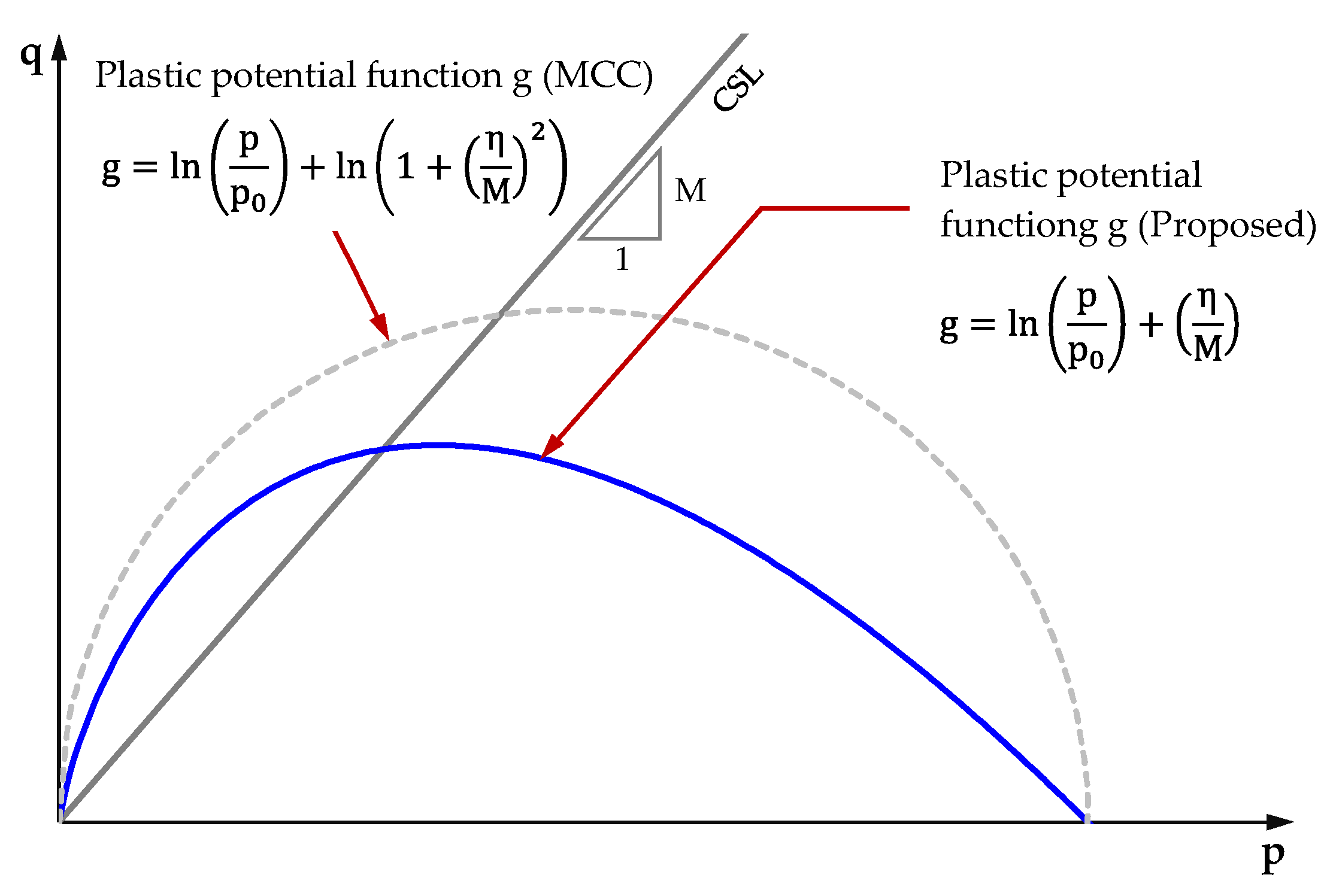
Figure 3.
Effects of on shape of yield function and stress path for NC clay: (a) yield function curves for different values of ; (b) stress path for NC clay on p-q plane against values of .
Figure 3.
Effects of on shape of yield function and stress path for NC clay: (a) yield function curves for different values of ; (b) stress path for NC clay on p-q plane against values of .
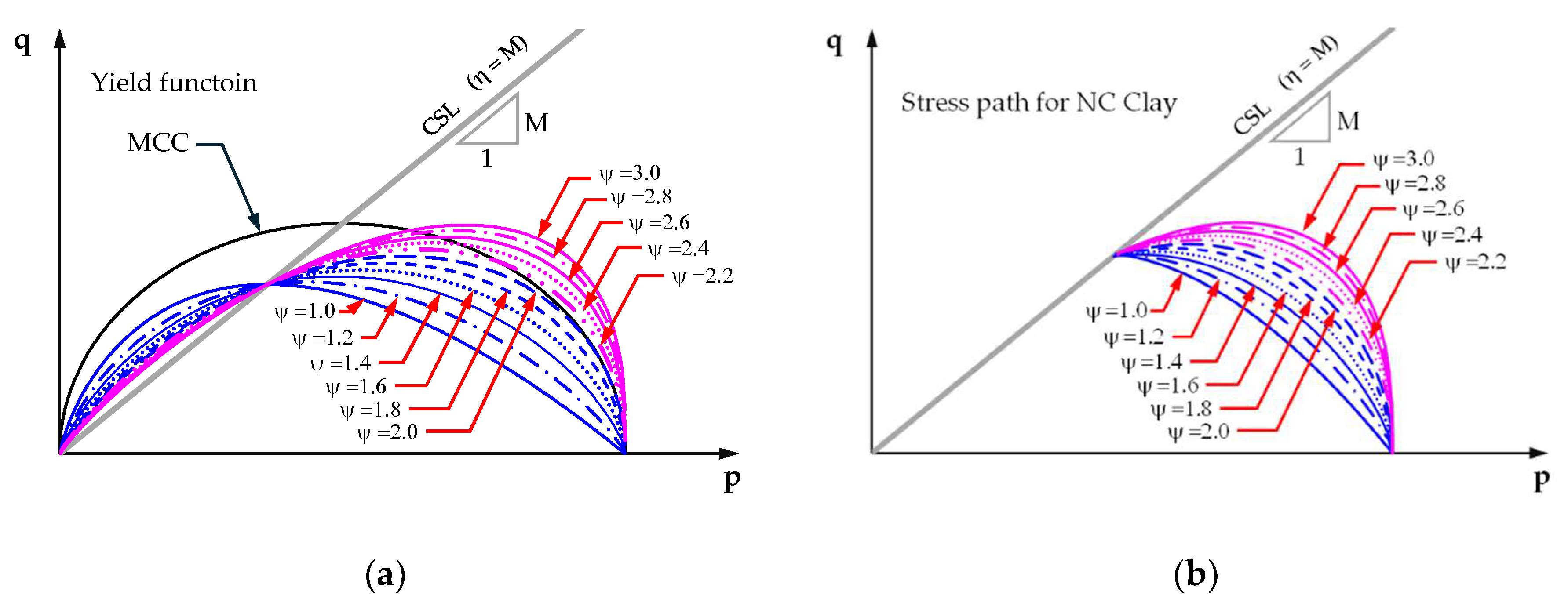
Figure 4.
Yield function f and plastic potential function g pairs adopted in this study: (a) for LPLS; (b) for HPLS.
Figure 4.
Yield function f and plastic potential function g pairs adopted in this study: (a) for LPLS; (b) for HPLS.
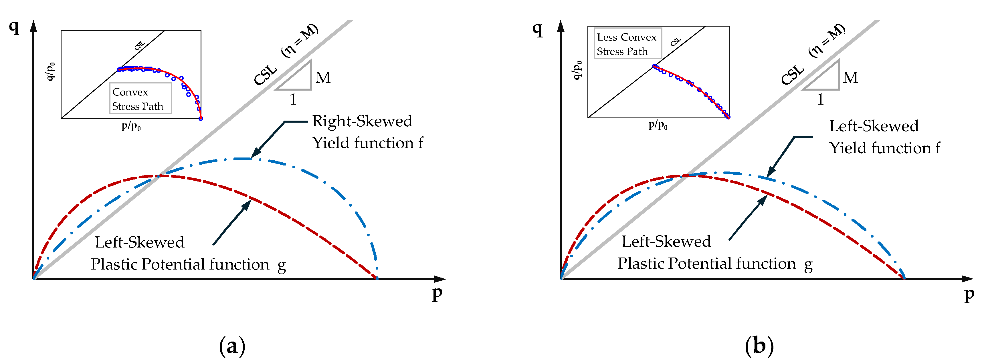
Figure 5.
Relationship between shape parameters , , and ().
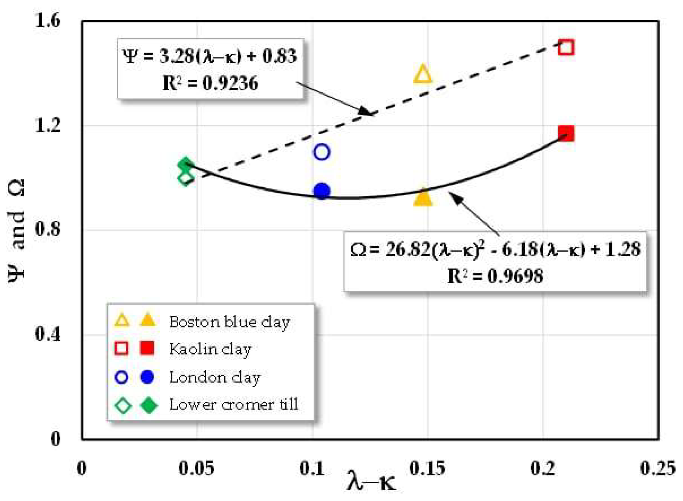
Figure 6.
Stress ratio–dilatancy relationships from experiments: (a) Fujinomori Clay [37]; (b) Lower Cromer till (LCT)[38].
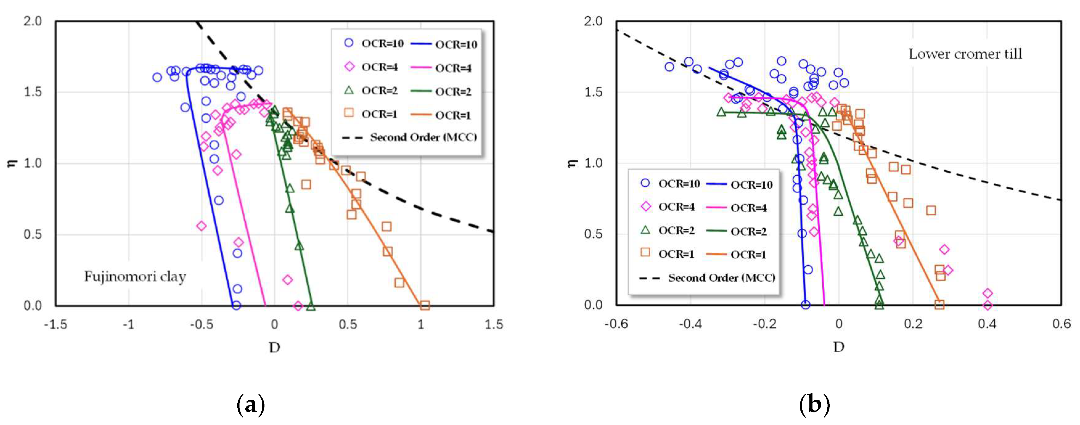
Figure 7.
Definition of the spacing ratio R.
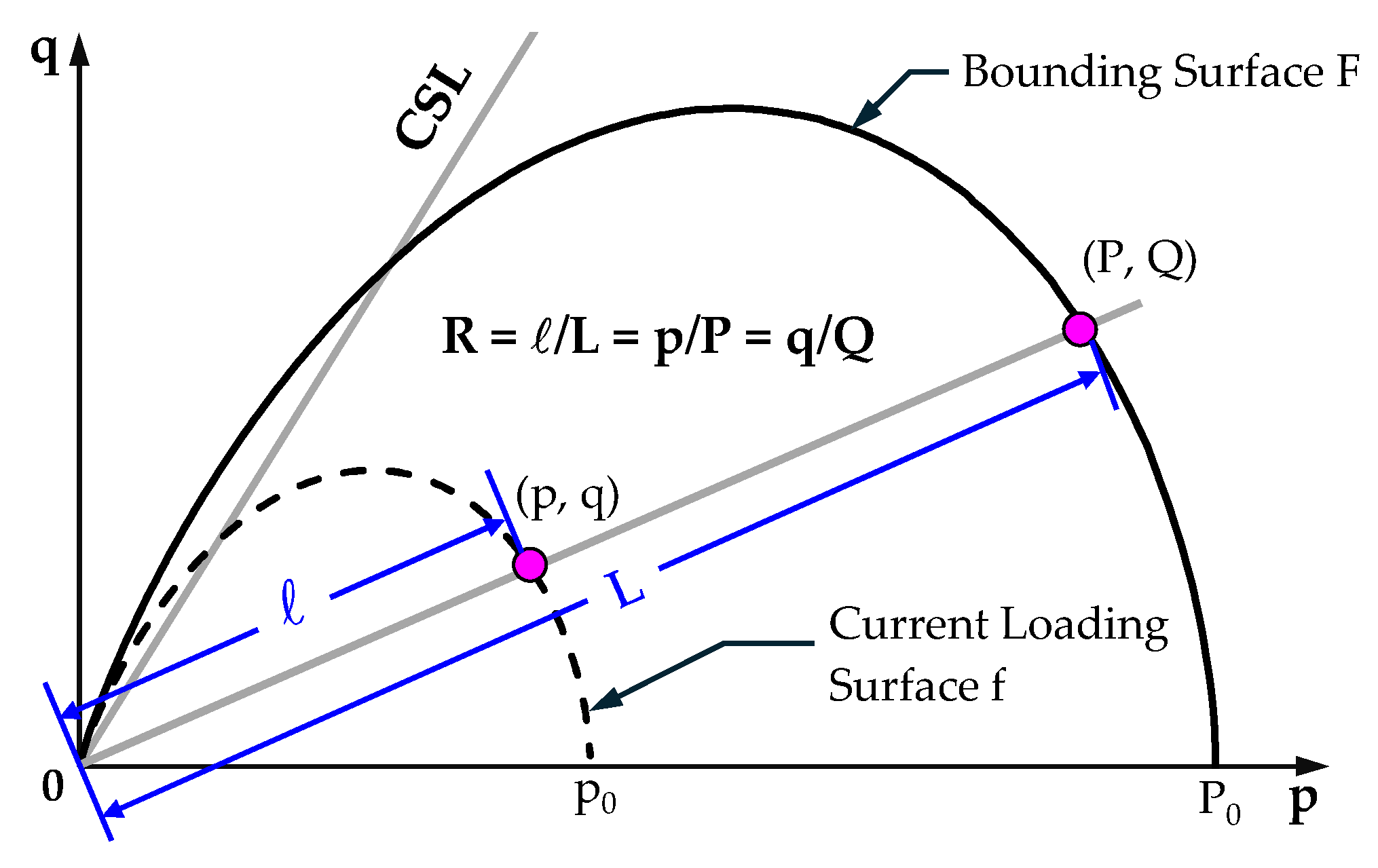
Figure 8.
Comparison of the disparity between drained and undrained stress path and shear strengths at the critical state for various OCR values.
Figure 8.
Comparison of the disparity between drained and undrained stress path and shear strengths at the critical state for various OCR values.
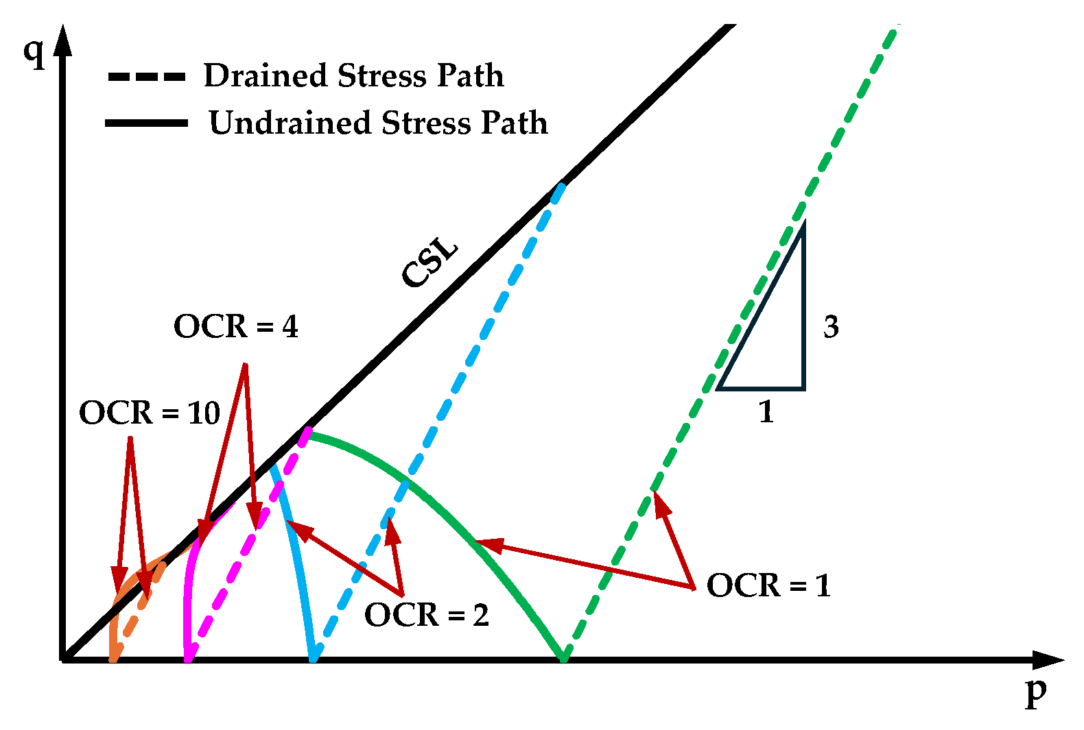
Figure 10.
Comparison of the failure envelopes of the Extended Mises and SMP criteria on the π-plane.
Figure 10.
Comparison of the failure envelopes of the Extended Mises and SMP criteria on the π-plane.
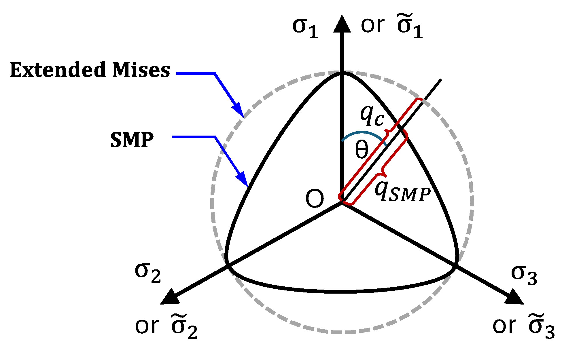
Figure 11.
Effects of parameter on normalized stress path (p′/ – q/) for various OCR.
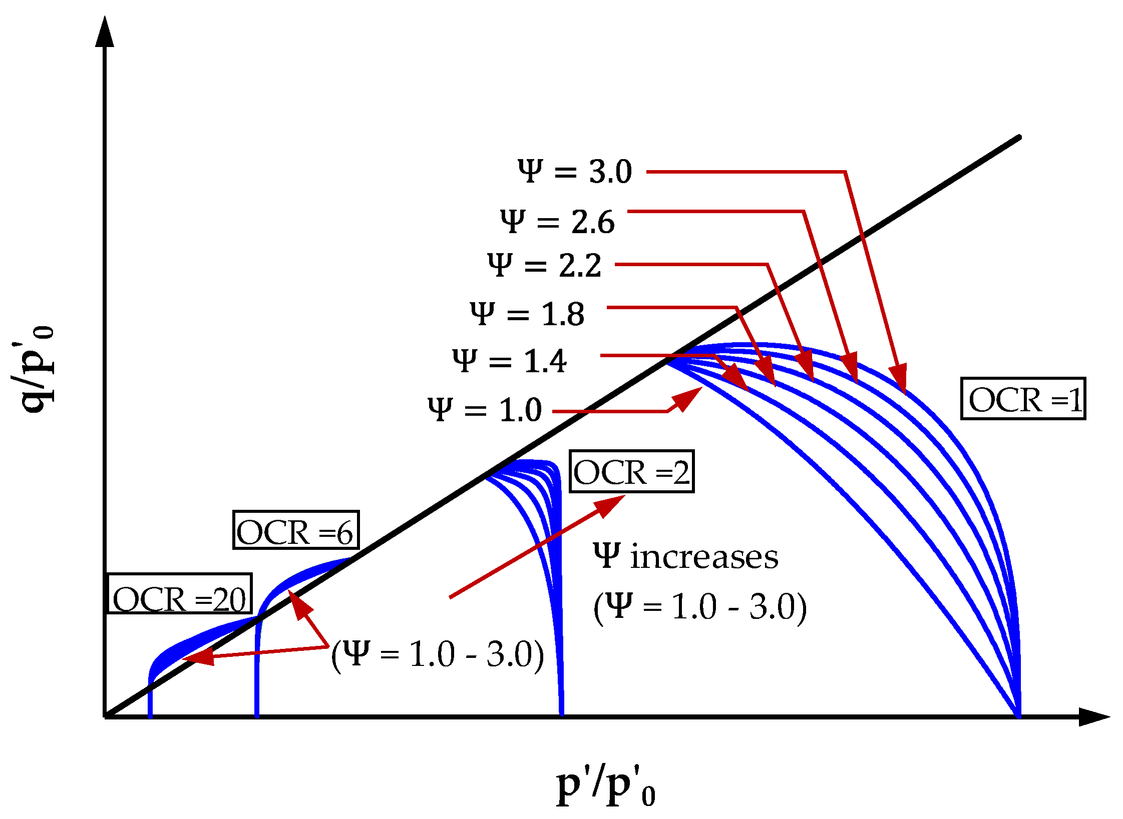
Figure 12.
Test results vs model predictions of London clay in undrained triaxial compression Test: (a-b) model I (proposed model); (c-d) model II; and (e-f) model III.
Figure 12.
Test results vs model predictions of London clay in undrained triaxial compression Test: (a-b) model I (proposed model); (c-d) model II; and (e-f) model III.
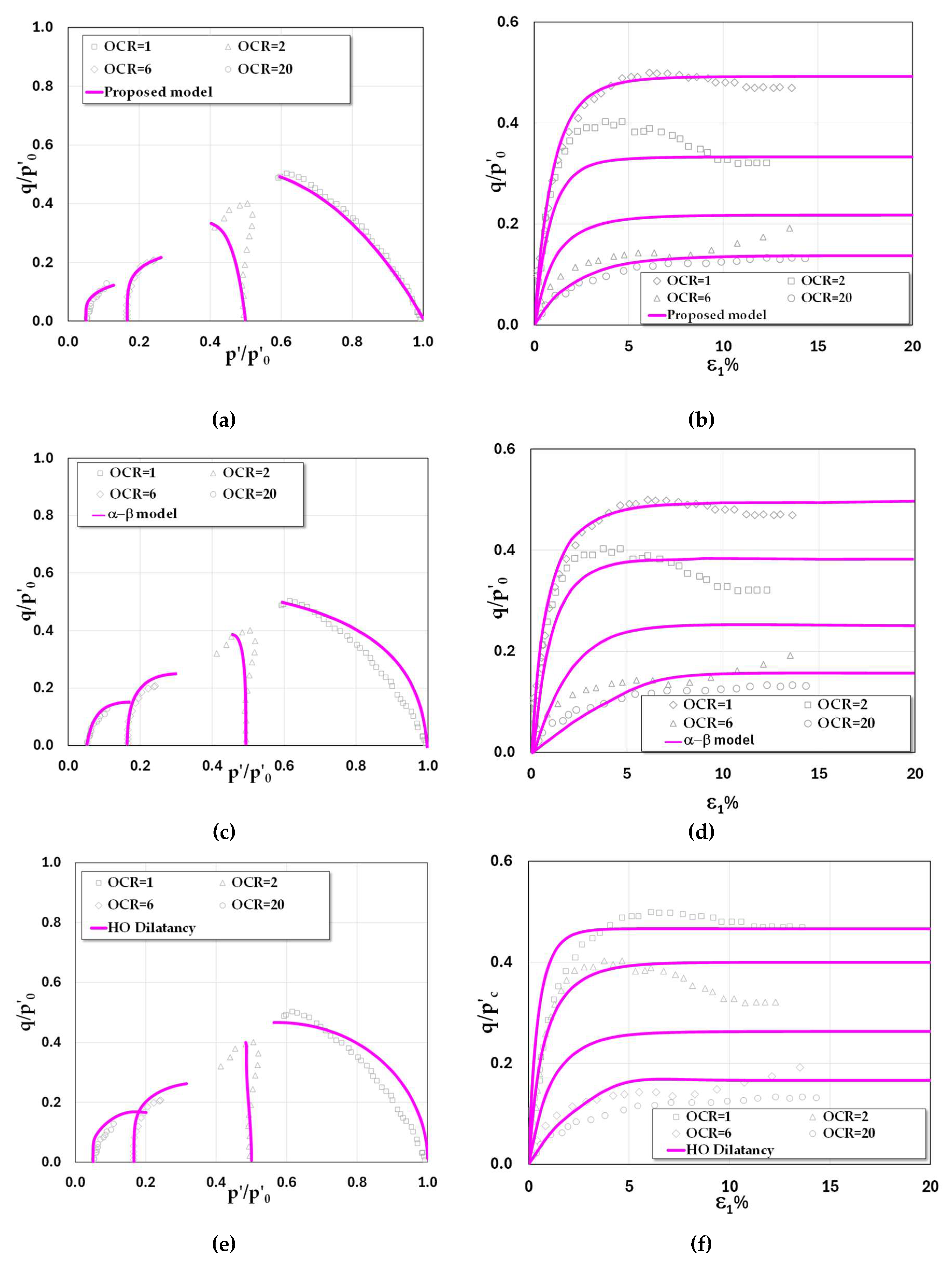
Figure 13.
Test results vs model predictions of Lower Cromer till in undrained triaxial compression Test: (a-b) model I (proposed model); (c-d) model II; and (e-f) model III.
Figure 13.
Test results vs model predictions of Lower Cromer till in undrained triaxial compression Test: (a-b) model I (proposed model); (c-d) model II; and (e-f) model III.
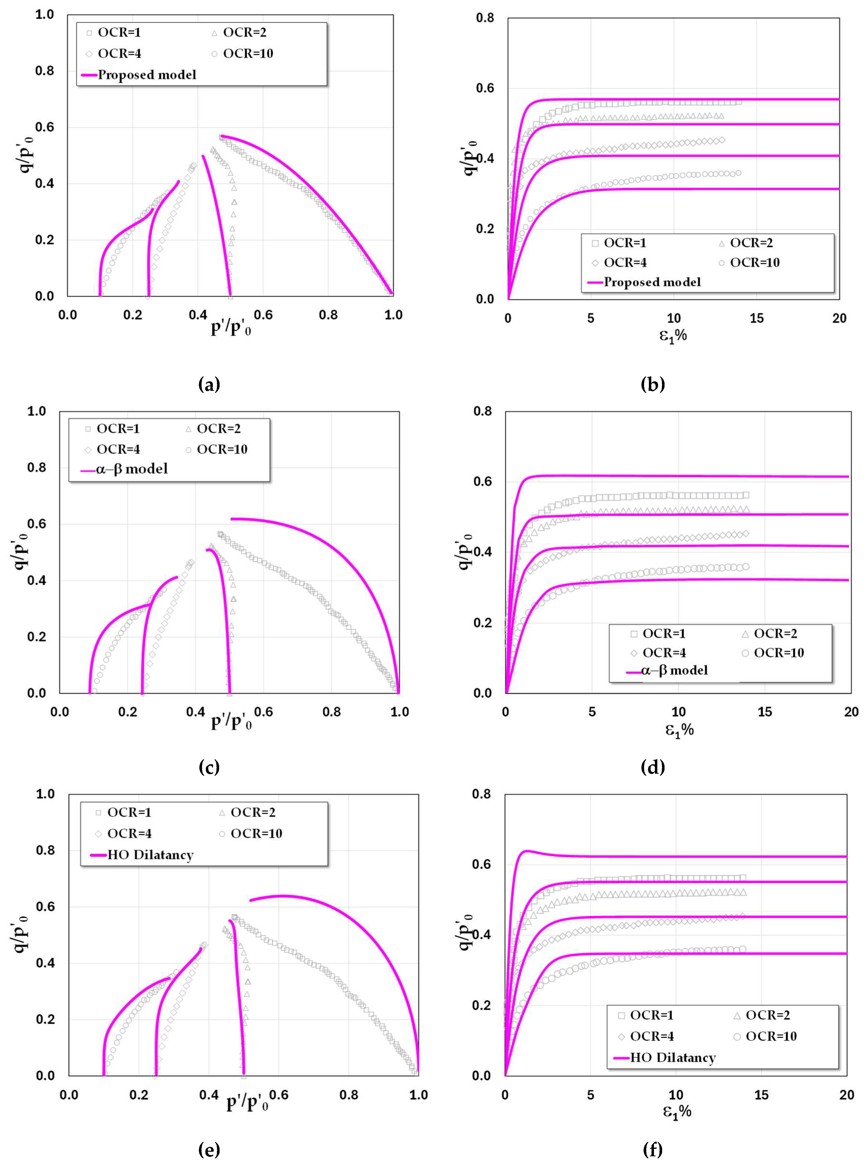
Figure 14.
Test results vs model predictions of Boston Blue clay in undrained triaxial compression Test: (a-b) model I (proposed model); (c-d) model II; and (e-f) model III.
Figure 14.
Test results vs model predictions of Boston Blue clay in undrained triaxial compression Test: (a-b) model I (proposed model); (c-d) model II; and (e-f) model III.
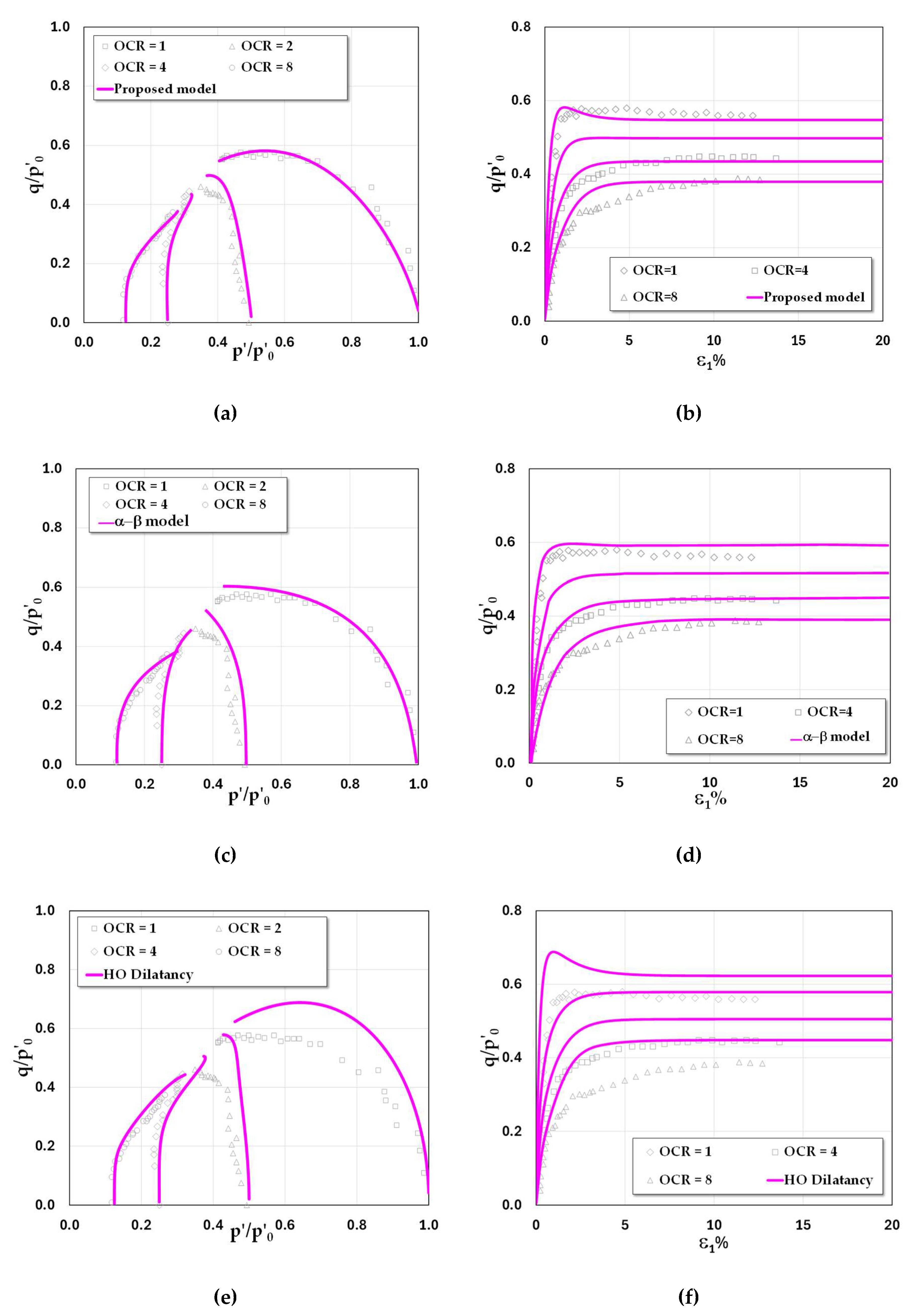
Figure 15.
Test results vs model predictions of Kaolin clay in undrained triaxial compression Test: (a-b) model I (proposed model); (c-d) model II; and (e-f) model III.
Figure 15.
Test results vs model predictions of Kaolin clay in undrained triaxial compression Test: (a-b) model I (proposed model); (c-d) model II; and (e-f) model III.
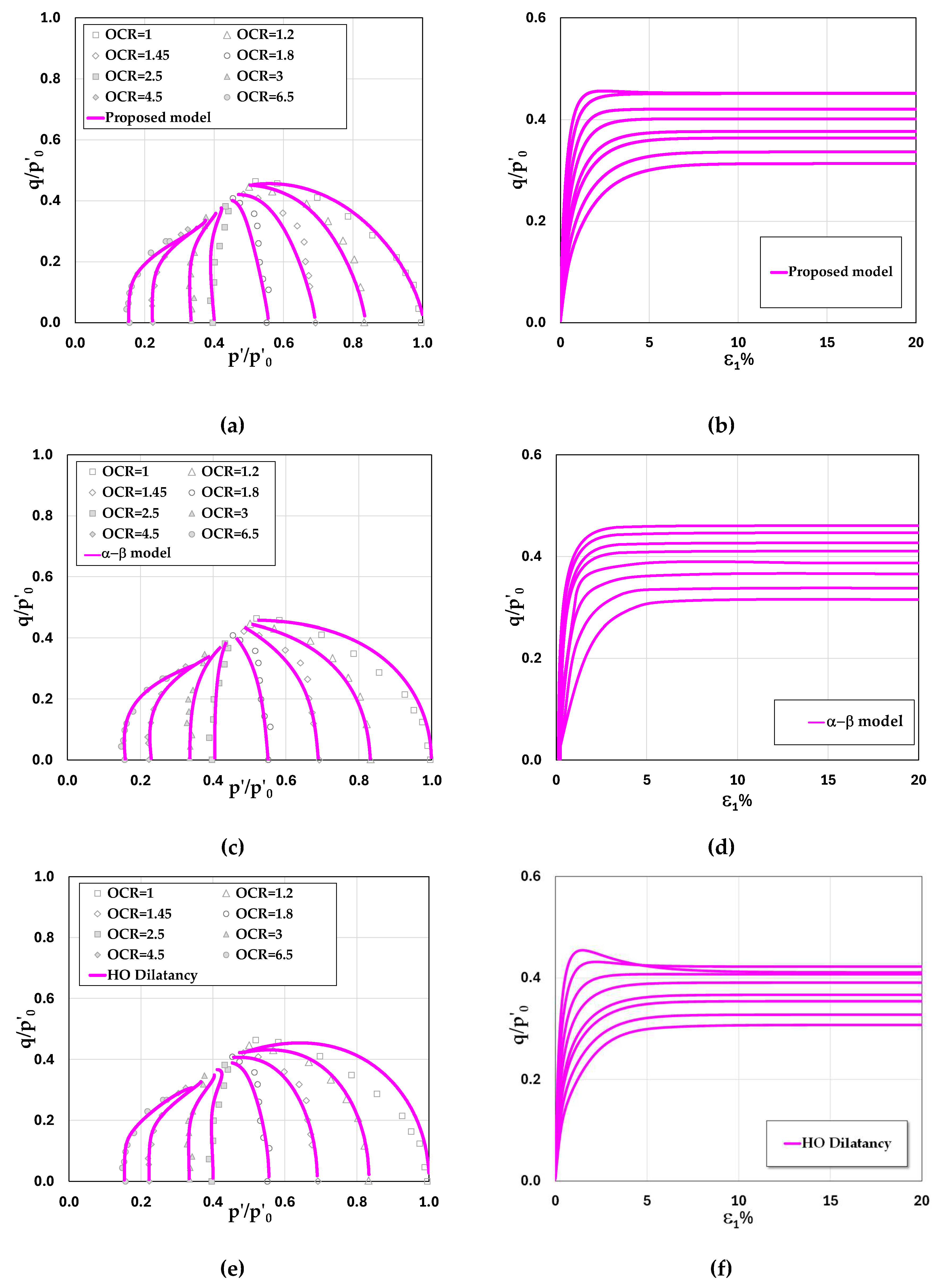
Figure 16.
Test results vs model predictions of Lower Cromer till in undrained triaxial extension Test: (a) normalized stress path (p/p0−q/p0); (b) stress-strain relations.
Figure 16.
Test results vs model predictions of Lower Cromer till in undrained triaxial extension Test: (a) normalized stress path (p/p0−q/p0); (b) stress-strain relations.
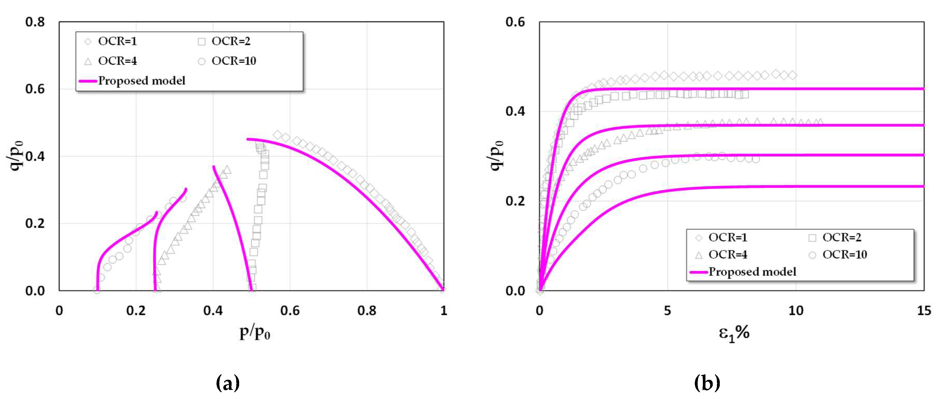
Figure 17.
Test results vs model predictions of Kaolin clay in undrained triaxial extension Test: (a) normalized stress path (p/p0−q/p0); (b) stress-strain relations.
Figure 17.
Test results vs model predictions of Kaolin clay in undrained triaxial extension Test: (a) normalized stress path (p/p0−q/p0); (b) stress-strain relations.
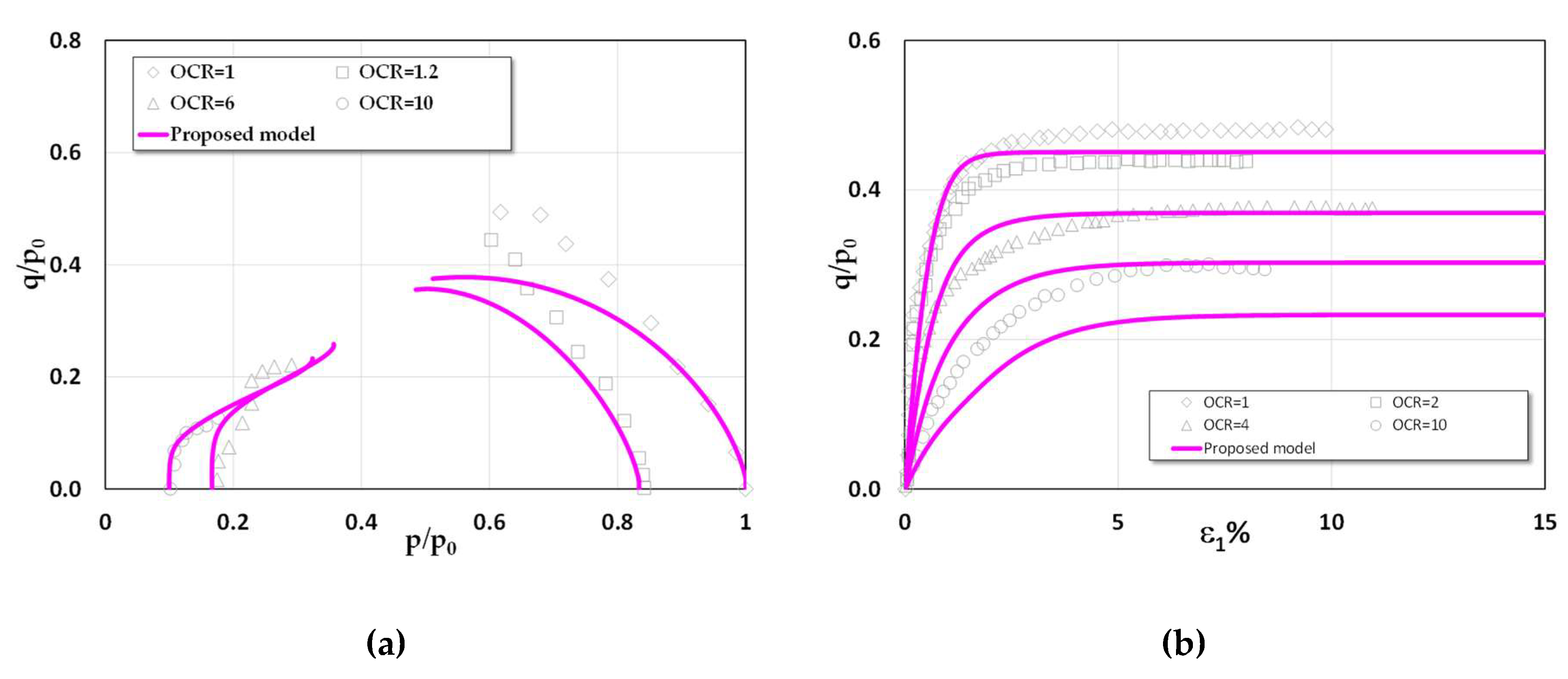
Figure 18.
Comparison between triaxial drained test results and model prediction of Lower Cromer till for different OCRs: (a) normalized effective stress paths; (b) stress–strain behavior.
Figure 18.
Comparison between triaxial drained test results and model prediction of Lower Cromer till for different OCRs: (a) normalized effective stress paths; (b) stress–strain behavior.
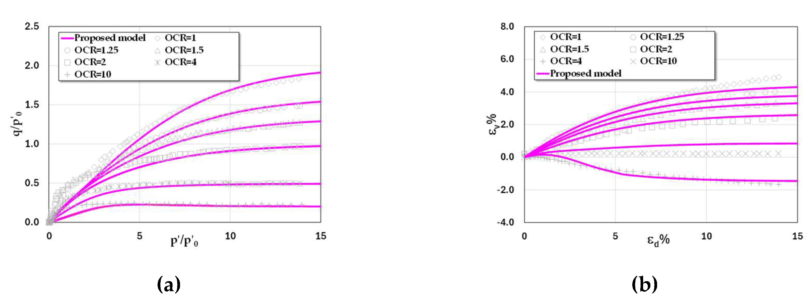
Figure 19.
Comparison between triaxial drained test results and model prediction of Fujinomori clay for different OCRs: (a) normalized effective stress paths; (b) stress–strain behavior.
Figure 19.
Comparison between triaxial drained test results and model prediction of Fujinomori clay for different OCRs: (a) normalized effective stress paths; (b) stress–strain behavior.
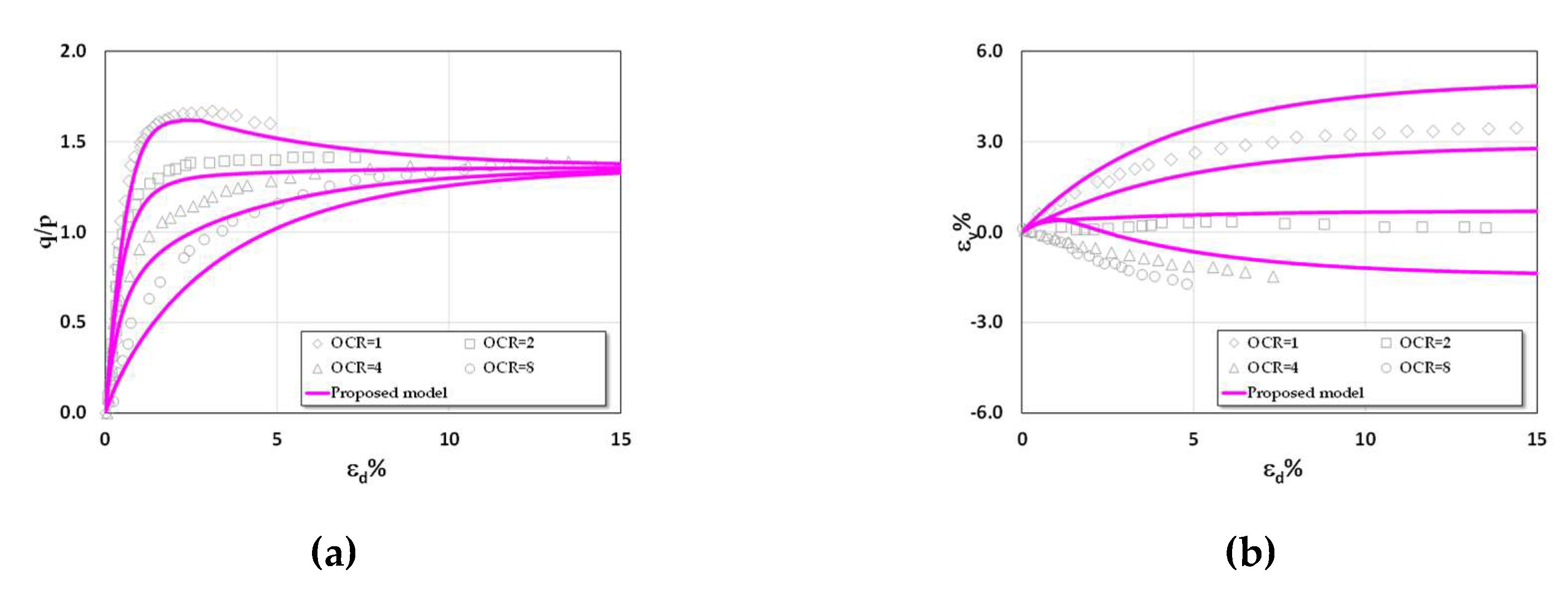
Figure 20.
Comparison between triaxial drained test results and model prediction of Shanghai clay for different OCRs: (a) normalized effective stress paths; (b) stress–strain behavior.
Figure 20.
Comparison between triaxial drained test results and model prediction of Shanghai clay for different OCRs: (a) normalized effective stress paths; (b) stress–strain behavior.
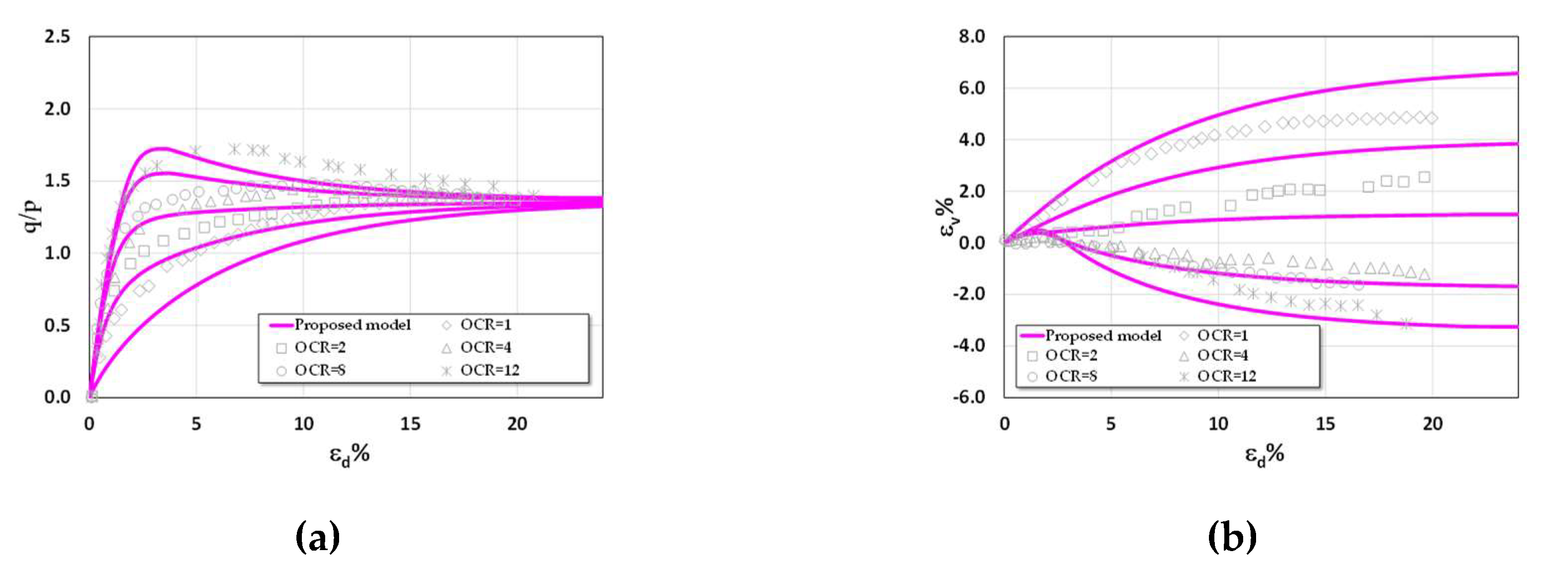

Table 1.
Soil parameters of the models used in the undrained analyses.
| Source of Clay | Basic Parameters | Extra Parameters | |||||||||||
|---|---|---|---|---|---|---|---|---|---|---|---|---|---|
| λ | κ | ν | Mc | e0 | Ψ1 | Ω1 | χ2 | β02 | n2 | α3 | β3 | ||
| London clay [40] | 0.168 | 0.064 | 0.25 | 0.827 | 1.843 | 1.1 | 0.95 | 0.2 | 1.0 | 1.0 | 0.8 | 1.0 | |
| Lower Comer till [38] | 0.063 | 0.018 | 0.30 | 1.200 | 0.747 | 1.0 | 1.05 | 0.2 | 1.0 | 0.8 | 0.7 | 1.0 | |
| Boston blue clay [41] | 0.184 | 0.036 | 0.10 | 1.353 | 2.059 | 1.4 | 0.93 | 0.3 | 1.0 | 1.0 | 0.7 | 0.5 | |
| Kaolin clay [42] | 0.260 | 0.050 | 0.20 | 0.896 | 2.957 | 1.5 | 1.17 | 0.3 | 1.0 | 1.2 | 0.8 | 1.0 | |
1 used in only model I (proposed model). 2 used in only model II (model proposed by Xu et al., 2024). 3 used in only model III (model proposed by Chen and Yang, 2017).
Disclaimer/Publisher’s Note: The statements, opinions and data contained in all publications are solely those of the individual author(s) and contributor(s) and not of MDPI and/or the editor(s). MDPI and/or the editor(s) disclaim responsibility for any injury to people or property resulting from any ideas, methods, instructions or products referred to in the content. |
© 2025 by the authors. Licensee MDPI, Basel, Switzerland. This article is an open access article distributed under the terms and conditions of the Creative Commons Attribution (CC BY) license (http://creativecommons.org/licenses/by/4.0/).
Copyright: This open access article is published under a Creative Commons CC BY 4.0 license, which permit the free download, distribution, and reuse, provided that the author and preprint are cited in any reuse.


