
Submitted:
24 March 2025
Posted:
25 March 2025
You are already at the latest version
Abstract
This study presents an improved analytical approach for one-dimensional consolidation settlement by introducing a revised AJOP (Arc Joint via Optimum Parameters) equation. This modified equation integrates both curved and linear segments within a unified framework, enhancing accuracy across varying stress levels for normally consolidated clay. Additionally, the revised AJOP function, coupled with newly proposed equations for symmetrical and asymmetrical hysteresis, improves the modeling of overconsolidated clay. The findings from a comparative investigation using conventional methods, including the linear function (LF) and the curved function (CF), reveal that LF significantly overestimates settlement, while CF, though accurate at shallow depths, introduces slight errors at greater depths. The revised AJOP equation effectively resolves these limitations. Furthermore, results highlight the crucial impact of clay layering techniques on consolidation settlement predictions. Non-layered models yield lower settlement estimates compared to multilayer approaches, emphasizing the significance of the proper e-logs'v relationship and layering techniques in enhancing prediction reliability.
Keywords:
Consolidation
; Settlement
; One-Dimensional
; Oedometer
; Non-linear
; Analytical Solution
; Closed-Form
; Normally Consolidated Clay
; Overconsolidated Clay
1. Introduction
Consolidation settlement is a crucial factor in the total settlement of clayey soils. If excessive, it can cause structural damage. This type of settlement occurs gradually as pore water dissipates from soil voids under applied loads, resulting in time-dependent deformation. It is crucial to predict the consolidation settlement with high accuracy, otherwise the error of the calculation can serve a considerable post-construction settlement and high maintenance cost. In the literatures, the method for calculating the consolidation settlement of clay at any given time after the application of a load can be calculated using the formula where represents the consolidation settlement at any time occurred after the load is applied, is the total consolidation settlement, and U is the degree of consolidation. In order to calculate precisely, accurate values for both and U are required.
For the calculation of U, the non-linear consolidation theory was first proposed by Davis and Raymond [1]. It is predicted on the ideas that the initial effective stress remains constant with depth and the permeability is proportional to the compressibility during the consolidation process [2,3]. Numerous attempts have been made to create various one-dimensional consolidation models that take into account the non-linear variations in permeability and compressibility [4,5,6,7,8,9,10,11,12,13,14,15,16,17,18,19,20]. Recently, Kim et al. (2021) [21] successfully in developing the analytical solution for U of multilayered soil under time-dependent loading. Based on this information, the calculation of U therefore has high accuracy. On the other hand, in literature, the calculation of still relies on an approximation method. This method is based on a linear relationship between the void ratio () and effective vertical stress () derived from the one-dimensional consolidation tests conducted in the laboratory. In soil mechanics, two types of clay were explained via : Normally Consolidated Clay (NC), which is clay where the current stress is the highest it has ever been, and Overconsolidated Clay (OC), which is clay that has experienced higher stress in the past than the current stress (e.g., [22,23,24]). The virgin compression line (VCL) is defined as the portion of the graph that represents NC. Additionally, in the experiment, there will be parts of the graph showing unloading and reloading portions (referred as the hysteresis), both of them represent OC. Although the test results are non-linear, the calculation method assumes linear approximation for both the VCL and the hysteresis for simplicity. The equations used to calculate consolidation settlement based on this approximation, which applies to the difference in void ratio () from the experimental result graphs, are presented in Equations 1-2 (e.g., [25]). This approximation contributes to the ongoing inaccuracy in calculating consolidation settlement and .
Normally Consolidated clay:
Overconsolidated clay:
In Equations 1-2, is the soil layer’s thickness, is the initial void ratio, is the effective overburden stress, is the maximum past pressure, and is the stress increment due to surface loading.
To address the inaccuracies in calculating consolidation settlement, it is essential to use appropriate equations for the curve rather than relying on linear approximations. In literature, the relationship between and , where represents the mean effective stress, from one-dimensional consolidation tests is frequently utilized for modeling soils, including clay (e.g., [26,27,28,29,30,31,32]) and sand (e.g., [33,34,35,36,37,38,39]). A comprehensive review by Kaewhanam and Chaimoon (2023) [40] found that linear equations are accurate for high stress levels but tend to be quite inaccurate at lower stress levels due to the curved nature of experimental results. In contrast, curved equations in the form of power functions, which are commonly used for granular soils, are accurate at lower stress levels because the experimental results follow a similar tendency. However, power functions can be significantly inaccurate at high stress levels as they cannot accurately represent a straight line. Additionally, Kaewhanam and Chaimoon (2023) [40] were the first to introduce an equation that combines a curve with a straight line on a semi-logarithmic scale, using only four fitting parameters. This approach can significantly reduce errors in calculating the changes in void ratio () for normally consolidated clay (NC). However, for calculations involving overconsolidated clay (OC), a non-linear hysteresis equation remains necessary.
Recent studies suggest that creep and consolidation can occur simultaneously [41,42,43,44], challenging earlier findings that creep follows consolidation [45,46,47]. However, these studies rely on linear consolidation principles, necessitating a refined framework that separates consolidation from creep before integration. Field experiments, such as the Väsby Test Fill in Sweden [48], confirm that consolidation and creep settlement occur concurrently, with creep continuing beyond primary consolidation. A key concern is the sensitivity of clay, typically defined as which influences stress-strain behavior and can cause discrepancies between lab and field results. Leroueil et al. (1985) [49] addressed this issue by incorporating time and strain rate into the relationship, leading to a more consistent stress-strain correlation for sensitive clays. However, for non-sensitive clays, traditional methods remain applicable.
This study develops an analytical solution for consolidation settlement () independent of creep for both NC and OC clays. To achieve this, we: (1) refine Kaewhanam and Chaimoon’s (2023) equation to better model the relationship for NC clays, and (2) introduce new equations to capture hysteresis behavior in OC clays. These refinements establish a closed-form solution for during loading, eliminating errors in consolidation settlement calculations in Equations 1-2.
2. Derivation of Equations for Laboratory Test Results
In this section, two advanced equations for arcs representing were developed: one for the virgin compression line (VCL) and one for the hysteresis. The specifics are described as the following.
2.1. Equation for the Virgin Compression Line (VCL)
As mentioned above, the equations for VCL found in the literature include both linear functions (LF) e.g., [26,27,28] and curved functions (CF) e.g., [33,34,35,36,37,38,39], as well as functions that combine both curved and linear segments in a single equation proposed by Kaewhanam and Chaimoon (2023) [40], referred to here as the Arc Joint via Optimum Parameters (AJOP). All these functions represent the relationship between the void ratio and the mean effective stress where and are the effective vertical and horizontal stress, respectively. The equations for LF, CF, and AJOP are given in Equations 3-5, respectively, and a comparison of these three graph lines is depicted in Figure 1.
From the comparison, the AJOP equation provides the most accurate results in both low and high stress levels. In this study, the AJOP equation is adopted, and it will be revised such that the independent variable (the variable on the horizontal axis of the graph) is made compatible with the consolidation test results. This aims to simplify and streamline the calculation process. Thus, is changed to , the reference pressure is changed to a reference positive value , and the log is changed to the natural logarithm ln.
The revised AJOP equation is shown in Equation 6. The new fitting parameters of AJOP equation become , , and . According to the explanation in [40], and control the vertical shift and the horizontal shift of the graph, respectively. While controls the slope of the linear portion, control the curvature of the curved portion. The secant slope of the AJOP function can be determined using Equation 7. This equation provides an accurate calculation of between two points on VCL for normally consolidated clay without the estimation. Figure 2 shows the AJOP graph for the effects of various fitting parameters.
In Equation 7, and represent the vertical effective stresses at the initial point of stress interval (lower value) and the final point of interval (higher value), respectively, and . The changes in between these two points can be calculated by multiplying in Equation 7 by .
The application of the AJOP equation and its secant slope for calculating settlement in normally consolidated clays is straightforward. By substituting in Equation 1 with in Equation 7, the errors in the calculation can be effectively eliminated across all soil depths. It is worth to note that the traditional method, which relies on linear approximation and a constant , often results in significant calculation errors, particularly for shallow soils near the ground surface and these errors tend to decrease with depth. This discrepancy arises because the initial stress near the surface is relatively low, resulting in the initial stress point, located on the curved portion of the rather than on the straight portion. In addition, the stress induced by the surface loads is comparatively higher when compared to deeper soil layers. Therefore, application of the LF causes dramatic error of . When comparing the capabilities of the AJOP and CF equations, it becomes evident that CF can address the aforementioned issues similarly to AJOP. However, the use of CF introduces significant computational errors at greater depths due to the absence of a linear segment in its graph. At these greater depths, the stress induced by surface loads is relatively minor, it implies that the resulting errors have less impact compared to those of LF at shallower depths.
2.2. Equations for the Hysteresis
Hysteresis refers to a loop involving unloading followed by reloading in the consolidation test result of all clays due to the requirements in the experimental standard. This is to observe the reversible and irreversible deformation of clays during loading. In some clays, the unloading and reloading curves may overlap or closely align, allowing the hysteresis can be simplified using a straight line with a constant slope . In such a situation, calculations using the linear approximation can provide accuracy for overconsolidated clays. However, some clays exhibited differently such as clays in [22,23,24] which is evident that the unloading and reloading curves deviate significantly. For these clays, the secant slope between two points on the unloading or reloading curves differed to the value of the average value . Therefore, the existing linear approximation method cannot provide high accuracy for these clays. To address this, adopting an equation capable of representing both types of hysteresis behavior could improve the accuracy of settlement calculations in overconsolidated clays. This approach enhances the precision of modeling soil compression and helps in predicting deformation under varying loading conditions more reliably.
Additionally, it was found that some hysteresis can be both symmetric and asymmetric. Symmetric hysteresis refers to cases where the reloading curve returns a point close to the starting point of the unloading curve on VCL. However, certain clays exhibit different characteristics, specifically asymmetric hysteresis, where the reloading curve bends below the starting point of the unloading curve on VCL. This behavior contributes to the increased occurrence of irreversible strain in overconsolidated clays, which tend to experience greater water expulsion than usual.
It is necessary to consider both accuracy and ease of use in order to create equations that correctly depict the unloading-reloading part. In this study, parabolic equations are employed. Generally, three fitting parameters are used for a parabola, as shown in Equation 8. An upward-facing parabolic equation represents the unloading phase (with parameters , and ), while a downward-facing parabolic equation represents the reloading phase of the experimental results (with different parameters , and ). It should be noted that Equation 8 can be valid for the unloading only if is less than or equal to the stress at the unloading point on VCL. Figure 3 illustrates the concept of using parabolas to describe the unloading-reloading graphs.
It is crucial to first formulate an equation to represent symmetric hysteresis behavior. Once this foundational equation is established, it can be further revised to accommodate asymmetric hysteresis. This approach ensures systematic progression from simpler to more complex representations of hysteresis, enhancing the ability to accurately model and predict soil behavior under varying conditions.
2.2.1. Equations for the Symetric Hysteresis
For symmetric hysteresis, three parameters (, and ) should be applicable to both the upward-facing and downward-facing parabolas for simplicity. Therefore, it is necessary to derive the values of , and for the downward-facing parabola based on the values of , and of the upward-facing parabola.
Based on Equation 8, which is the equation for the unloading curve, the change in void ratio and the secant slope between the starting point of unloading (and any point on the symmetrical unloading () can be calculated using Equations 9-10, respectively.
In the case of symmetric hysteresis, the size of the upward parabolas used to represent the unloading and reloading curves is identical. Consequently, the parameter can be expressed in terms of . Next, to determine the formulas for and , it is necessary to set up two additional conditions. From Figure 3, it can be observed that the reloading line intersects two key points i.e., the point where unloading begins and the point where reloading begins . We use the coordinates of these two points to find and . First, determine the void ratio at both points by substituting the stress into the VCL equation (Equation 6) to obtain . Then, substitute the stress value at the reloading start point into the unloading equation (Equation 8) to obtain . Using the condition that for both calculations, by solving the simultaneous equations, we can derive formulas for and that depend on the four parameters of the newly proposed VCL (, as well as , , and . The equations for , and of the downward-facing parabola are shown in Equations 11 - 13, respectively.
where and .
At this step of the optimum parameter technique, a complete symmetric hysteresis (both unloading and reloading phases) can be evaluated using only three parameters (, and ). Furthermore, the tangent slope of the unloading portion in Equation 8 can be expressed in Equation 14. At the starting point of unloading (and on VCL) the tangent slope is usually assumed to be a constant for each type of soil. Therefore, can be determined by substituting in Equation 14 with as shown in Equation 15.
To calculate the and for the reloading of the symmetric hysteresis, substitute , and from Equations 11-13 in place of , and , and in place of in Equations 14-15, respectively. It should be noted that for the symmetric hysteresis, at on unloading curve is equal to at on reloading curve.
It is important to note that the reloading equation (Equation 14) is applicable only for and is limited by the stress on the VCL. Additionally, when , the asymmetric hysteresis becomes a symmetric hysteresis.
The change in void ratio and the secant slope between the starting point of reloading (and any point on the symmetrical reloading () of Equation 8 can be calculated using Equations 16-17, respectively.
For overconsolidated clays exhibiting symmetrical hysteresis, the application of in the settlement calculations can be achieved by substituting with (as defined in Equation 17) and replacing with (as defined in Equation 7) simultaneously into Equation 2.
2.2.2. Equations for the Asymetric Hysteresis
The general characteristics of asymmetric hysteresis are illustrated in Figure 4. While the unloading portion is still the same as the symmetric hysteresis, the reloading curve distinctly slopes downward at the end compared to the symmetric hysteresis case. In this study, we introduce only one additional variable to the equation of symmetric hysteresis to become asymmetric hysteresis.
Equation 18 shows the relationship used to represent the reloading curve for both symmetric () and asymmetric () hysteresis which is valid only for stress that does not exceed the stress value on the AJOP line. Notably, the value of term in Equation 18 will be equal to 1 when stress point is on the starting point of reloading. This results in the slope at this point remaining the same as for the symmetric reloading curves.
The change in void ratio and the secant slope between the starting point of reloading (and any point on the asymmetrical reloading () of Equation 18 can be calculated using Equations 19-20, respectively.
It is important to note that the loading behavior of overconsolidated clay from the initial stress to the final stress can be divided into two cases: 1) when , remains on the reloading curve as shown in Figure 5a, therefore settlement can be directly calculated using in Equation 19; and 2) when , thus shifts to the VCL as shown in Figure 5b, and the settlement could be calculated using in Equation 21. This distinction ensures accurate settlement calculations under different loading conditions. Using Equations 19 or 21, the error of in the approximation by LF can be eliminated.
Although , , , and are derived from the laboratory test results, these parameters can also be applied to the unloading at other stress values without graph refit. The values of ′, ′, and ′ for unloading at other points on the VCL can be calculated from the values of , , and at by assuming that: 1) the parabola for the unloading portion retains the same size, i.e., ′= , and 2) the tangent slope of the unloading line at the start of unloading remains constant for every unloading points. Thus, from Equation 8, ′ is given by and where and are the stress and void ratio at the new unloading point, respectively. Furthermore, when dealing with the reloading from the end point of this new unloading, the procedure of ′, ′ and ’ for the reloading can be determined by the equations mentioned above.
3. The Process of Calculating One-Dimensional Consolidation Settlement
The short description for calculating the consolidation settlement can be summarized as follows:
- Fit the experimental consolidation data to the VCL using AJOP equation (Equation 6) to obtain four parameters and .
- Fit the experimental consolidation data using Equation 8 to obtain three parameters for the upward-facing parabola (unloading portion) , , and .
- Fit the experimental consolidation data using Equation 18 to obtain a parameter for the downward-facing parabola (reloading portion). ( for symmetric hysteresis).
- Divide the soil to be analyzed for settlement into the sublayers.
- Determine the initial and the final stresses resulting from construction at the middle point of each layer. The elastic solution can be used for simplification.
-
For the overconsolidated clay, it is necessary to calculate more steps as follows:6.1) Calculate the maximum past stress which will be used as the unloading point on the VCL of each layer.6.2) Calculate the void ratio of the unloading point at in the step 6.1) using AJOP equation.6.3) Determine the parameters (′, ′ and ′) (, and ) of the unloading of each midpoint.6.4) Calculate the void ratio of the initial stress which will be the same value of the void ratio of the starting point of reloading process .6.5) Determine the parameters (′, ′ and ’) (, and ) of the reloading of each mid-point.
-
Calculate between the initial and final stresses mentioned above in step 5 as follows:7.1) For NC (normally consolidated) clay: use Equation 7.7.2) For OC (overconsolidated) clay: use Equation 19 or 21.
- Calculate the consolidation settlement of the layer using
- The total consolidation settlement can be calculated as the sum of the settlements for each individual layer i.e., when n is the number of soil layers.
4. Examples for the Prediction of One-Dimensional Consolidation Settlement
To demonstrate the performance of the newly proposed equations, the examples of the calculation for total consolidation settlement () will be applied in the case of rectangular footing in size of 15m x 30m and clay thickness of 12m in this section. Three cases of analyses include
a) Single layer of clay.
b) Calculation by dividing the clay layer into layers, with each layer having a uniform thickness of 1m.
c) Calculation by dividing the clay into layers of varying thicknesses, applying the layers closer to the surface being thinner in conjunction to the thickness increasing with depth.
Three soil test data from distinct continents for the consolidation test (i.e., Bangkok Clay [22], Boston Blue Clay [23] and London Clay [24]) were used. Figure 6, Figure 7 and Figure 8 depict the test results from [22,23,24] with the best fit curves. Prior to the analysis, the soil parameters based on proposed method were extracted. Table 1 summarizes the fitting parameters for all three clays mentioned above. The parameters and are for the AJOP equation, and , , and are for the hysteresis portion. In the analysis of normally consolidated clay, three types of equations were applied LF, CF and AJOP. Figure 9, Figure 10 and Figure 11 show the problems to be analyzed for case a) single layer, b) equal layer thickness and c) varied layer thickness, respectively. It should be noted that all clays behave with asymmetrical hysteresis ().
Table 2 shows the results of settlement calculations based on the aforementioned methods and conditions of the normally consolidated clay. It is evident that the settlement from the LF is much greater than those from the CF and AJOP because the actual initial stress on the shallow points is not located on the straight line of . Therefore, the equations which provide the curved portion, i.e., CF and AJOP give lower value and give more reliable results. It is also indicating from Table 2 that the results from CF and AJOP are close together, due to the impact of error on deeper depts are less than the impact at shallow depts. In addition, when the method of layer dividing is considered, the results using single layer give lowest value for all clays and all models. The results from equal layer thickness model are close to the results for the method of varying layer thickness for all clays.
For the overconsolidated clay, the analyses are divided into two cases i.e., 1) low surface loading 200 kN/m2, and 2) high surface loading 1,000 kN/m2. Table 3 and Table 4 present the consolidation calculation results for overconsolidated clay in case 1) and case 2), respectively. From Table 3, the AJOP method is selected and is identified as the most reliable approach. The findings highlight the significant influence of the layer division method on the results. While using the AJOP equation, the single-layer division method yields the lowest settlement due to the mid-layer being positioned farther from the ground surface. On the other hand, the multilayer division method provides more accurate results because the mid-points of some layers are closer to the ground surface, which is a critical factor for the AJOP method. In case c), where layer thickness varies, the results are most accurate as the mid-points of the layers are correctly positioned. This demonstrates that both the calculation method and the layer division approach significantly affect the accuracy of the results. It should be noted that for this low surface loading value, we found that some soil layers were calculated with a final stress lower than the maximum past pressure.
Table 4 presents the calculation results under high loading conditions. In these calculations, both the compression ratio and the compression index were used for Boston and Bangkok clays. However, for London Clay, only the compression ratio was utilized in the calculations in some depths. The findings show that although using different methods in layer division, the consolidation settlement is similar for all methods with the fact that single layer expresses the lowest value.
5. Conclusions
The total amount of consolidation settlement in field can be determined by the changes in void ratio based on the clay characteristics evaluated from laboratory. This study proposed new equations that can fit well to the consolidation curve without any approximation and additional testing. The proposed equations include 1) the revised version of the AJOP for normally consolidated clay, and 2) equation for both symmetrical and asymmetrical hysteresis of overconsolidated clay. With these equations, the analytical solution for consolidation settlement for clays can be established.
A comparison between the existing methods and the proposed method was investigated. Three methods of the calculation include linear function (LF), curve function (CF) and the revised AJOP equation (function for curve and linear portions in a single equation). In addition, three models of clay layering are investigated, i.e., single layer, multilayers with equal and varied thickness. Three clay data from different continents were used in the analysis, i.e., Bangkok clay, Boston Blue clay and London clay.
For normally consolidated clay, it is revealed that the LF method yields significantly higher consolidation settlement compared to the CF and AJOP methods for all clays and all layering conditions. Additionally, the single-layer model gives lower consolidation settlement than both layered soil models. These phenomena are influenced by two key factors: 1) the presence of curved portion in , and 2) the omission and commission of curved portion in calculations due to the soil layering method. Therefore, the CF method provides greater accuracy than the LF method because the curved portion exists in CF. However, AJOP method reduces errors at both shallow and greater depths, as it incorporates both curved and linear segments within a single equation. For overconsolidated clay, only AJOP equation was selected in the analysis. The calculations yield similar results across all models. However, all soil samples indicate that the non-layered soil model results in slightly lower settlement compared to the other two methods.
The findings highlight the significance of accurately modeling of the void ratio and effective vertical stress relationship, particularly through a novel equation AJOP that combines curved and straight-line representation on a semi-logarithmic scale. This approach addresses the limitations of traditional methods, which often fail to capture the complexities of soil behavior at varying stress levels. Additionally, the authors have provided the recommendations in case of sample disturbance and sensitive clay are encountered. The proposed method not only enhances the understanding of consolidation processes but also provides a practical tool for engineers in predicting settlement behavior more reliably. Future work may focus on refining the method and exploring its applicability to a broader range such as consolidation-creep framework and constitutive model of clay.
Author Contributions
Conceptualization, N.K., N.A., S.S., A.U., N.S. and N.P.; methodology, N.K., N.S. and N.P.; software, N.P. and T.C.; validation, T.C., N.P., A.U.,N.S. and N.K.; formal analysis, N.P., T.C. and N.K.; investigation, N.P. and N.K.; resources, N.P.; data curation, N.P, T.C., N.A., S.S. and N.K.; writing—original draft preparation, N.P., T.C., A.U., S.S., N.A., N.S. and N.K.; writing—review and editing, N.P., T.C., A.U., S.S., N.A., N.S. and N.K.; visualization, A.U., S.S., N.A., N.S. and N.K.; supervision, A.U.,N.A., S.S., N.S. and N.K.; project administration, N.K.; funding acquisition, N.K. All authors have read and agreed to the published version of the manuscript.
Funding
Please add: This research was financially supported by Mahasarakham University, grant number 6717028/2567.
Data Availability Statement
The data presented in this study are available on request.
Acknowledgments
This research was supported by Mahasarakham University. The support is gratefully acknowledged.
Conflicts of Interest
The authors declare no conflicts of interest.
References
- Davis, E.H.; Raymond, G.P. A Non-Linear Theory of Consolidation. Geotech. 1965, 15, 161–173. [Google Scholar] [CrossRef]
- Barden, L.; Berry, P.L. Consolidation of Normally Consolidated Clay. J. Soil Mech. Found. Div. 1965, 91, 15–35. [Google Scholar] [CrossRef]
- Gibson, R.E.; England, G.L.; Hussey, M.J.L. The Theory of One-Dimensional Consolidation of Saturated Clays I, finite non-linear consolidation of thin homogeneous layers. Géotechnique 1967, 17, 261–273. [Google Scholar] [CrossRef]
- Gray, H. Simultaneous consolidation of contiguous layers of unlike compressive soils. ASCE Trans. 1945, 110, 1327–1356. [Google Scholar]
- Poskitt, T.J. The Consolidation of Saturated Clay with Variable Permeability and Compressibility. Geotech. 1969, 19, 234–252. [Google Scholar] [CrossRef]
- Schiffman, R.L.; Stein, J.R. One-Dimensional Consolidation of Layered Systems. J. Soil Mech. Found. Div. 1970, 96, 1499–1504. [Google Scholar] [CrossRef]
- Mesri, G.; Rokhasar, A. Theory of Consolidation for Clays. Geotech. Eng. Div. 1974, 100, 889–904. [Google Scholar] [CrossRef]
- Lee, P.K.K.; Xie, K.H.; Cheung, Y.K. A study on one-dimensional consolidation of layered systems. Int. J. Numer. Anal. Methods Géoméch. 1992, 16, 815–831. [Google Scholar] [CrossRef]
- Xie, K.; Pan, Q.Y. One-dimensional consolidation of soil stratum of arbitrary layers under time-dependent loading. China J. Geotech. Engng. 1995, 17, 82–87. [Google Scholar]
- Lekha, K.R.; Krishnaswamy, N.R.; Basak, P. Consolidation of Clays for Variable Permeability and Compressibility. J. Geotech. Geoenvironmental Eng. 2003, 129, 1001–1009. [Google Scholar] [CrossRef]
- Zhuang, Y.C.; Xie, X.B.; Li, J. Nonlinear analysis of consolidation with variable compressibility and permeability. J. Zhejiang Univ. 2005, 6, 181–187. [Google Scholar] [CrossRef]
- Abbasi, N.; Rahimi, H.; Javadi, A.A.; Fakher, A. Finite difference approach for consolidation with variable compressibility and permeability. Comput. Geotech. 2007, 34, 41–52. [Google Scholar] [CrossRef]
- Conte, E.; Troncone, A. Nonlinear consolidation of thin layers subjected to time-dependent loading. Can. Geotech. J. 2007, 44, 717–725. [Google Scholar] [CrossRef]
- Carrera, E.; Brischetto, S. Analysis of thickness locking in classical, refined and mixed multilayered plate theories. Compos. Struct. 2008, 82, 549–562. [Google Scholar] [CrossRef]
- Zheng, G.Y.; Li, P.; Zhao, C.Y. Analysis of non-linear consolidation of soft clay by differential quadrature method. Appl. Clay Sci. 2013, 79, 2–7. [Google Scholar] [CrossRef]
- Li, C.; Huang, J.; Wu, L.; Lu, J.; Xia, C. Approximate Analytical Solutions for One-Dimensional Consolidation of a Clay Layer with Variable Compressibility and Permeability under a Ramp Loading. Int. J. Géoméch. 2018, 18. [Google Scholar] [CrossRef]
- Xie, K.-H.; Xie, X.-Y.; Jiang, W. A study on one-dimensional nonlinear consolidation of double-layered soil. Comput. Geotech. 2002, 29, 151–168. [Google Scholar] [CrossRef]
- Chen, R.P.; Zhou, W.H.; Wang, H.Z.; Chen, Y.M. One-Dimensional Nonlinear Consolidation of Multi-Layered Soil by Dif-ferential Quadrature Method. Comput. Geotech. 2005, 32, 358–369. [Google Scholar] [CrossRef]
- Hu, J.; Bian, X.; Chen, Y. Nonlinear consolidation of multilayer soil under cyclic loadings. Eur. J. Environ. Civ. Eng. 2019, 25, 1042–1064. [Google Scholar] [CrossRef]
- Kim, P.; Ri, K.-S.; Kim, Y.-G.; Sin, K.-N.; Myong, H.-B.; Paek, C.-H. Nonlinear Consolidation Analysis of a Saturated Clay Layer with Variable Compressibility and Permeability under Various Cyclic Loadings. Int. J. Géoméch. 2020, 20, 04020111. [Google Scholar] [CrossRef]
- Kim, P.; Kim, H.-S.; Pak, C.-U.; Paek, C.-H.; Ri, G.-H.; Myong, H.-B. Analytical solution for one-dimensional nonlinear consolidation of saturated multi-layered soil under time-dependent loading. J. Ocean Eng. Sci. 2021, 6, 21–29. [Google Scholar] [CrossRef]
- Trani, L.; Bergado, D.; Abuel-Naga, H. Thermo-mechanical behavior of normally consolidated soft Bangkok clay. Int. J. Geotech. Eng. 2010, 4. [Google Scholar] [CrossRef]
- Whittle, A.J.; DeGroot, D.J.; Ladd, C.C.; Seah, T. Model Prediction of Anisotropic Behavior of Boston Blue Clay. J. Geotech. Eng. 1994, 120, 199–224. [Google Scholar] [CrossRef]
- Santos, L.M.; a Oliveira, P.J.; Sousa, J.N. V.; Lemos, L.J.L. Effect of Initial Stiffness on The Induced Horizontal Displacements of Geotechnical Structures Built on/in Overconsolidated Clays. International Society for Soil Mechanics and Geotechnical En-gineering, Imperial College London, United Kingdom, 26-28 June,2023.
- Aysen, A.; Popescu, M. Soil Mechanics: Basic Concepts and Engineering Applications. Appl. Mech. Rev. 2003, 56, B27–B27. [Google Scholar] [CrossRef]
- Matsuoka, H.; Yao, Y.-P.; Sun, D. The Cam-Clay Models Revised by the SMP Criterion. Soils Found. 1999, 39, 81–95. [Google Scholar] [CrossRef]
- Yao, Y.; Sun, D.; Luo, T. A critical state model for sands dependent on stress and density. Int. J. Numer. Anal. Methods Géoméch. 2004, 28, 323–337. [Google Scholar] [CrossRef]
- Yao, Y.; Sun, D.; Matsuoka, H. A unified constitutive model for both clay and sand with hardening parameter independent on stress path. Comput. Geotech. 2007, 35, 210–222. [Google Scholar] [CrossRef]
- Cao, L.F.; Teh, C.I.; Chang, M.F. Undrained Cavity Expansion in Modified Cam Clay I: Theoretical Analysis. Geotechnique. 2001, 51, 323–334. [Google Scholar] [CrossRef]
- Grimstad, G.; Degago, S.A.; Nordal, S.; Karstunen, M. Modeling creep and rate effects in structured anisotropic soft clays. Acta Geotech. 2010, 5, 69–81. [Google Scholar] [CrossRef]
- Yin, Z.-Y.; Xu, Q.; Hicher, P.-Y. A simple critical-state-based double-yield-surface model for clay behavior under complex loading. Acta Geotech. 2013, 8, 509–523. [Google Scholar] [CrossRef]
- Ou, C.Y.; Liu, C.C.; Chin, C.K. Anisotropic viscoplastic modeling of rate-dependent behavior of clay. Int. J. Numer. Anal. Methods Géoméch. 2010, 35, 1189–1206. [Google Scholar] [CrossRef]
- Li, X.S.; Wang, Y. Linear Representation of Steady-State Line for Sand. J. Geotech. Geoenvironmental Eng. 1998, 124, 1215–1217. [Google Scholar] [CrossRef]
- Yang, Z.X.; Li, X.S.; Yang, J. Quantifying and modelling fabric anisotropy of granular soils. Geotech. 2008, 58, 237–248. [Google Scholar] [CrossRef]
- Yang, J.; Wei, L.; Dai, B. State variables for silty sands: Global void ratio or skeleton void ratio? Soils Found. 2015, 55, 99–111. [Google Scholar] [CrossRef]
- Murthy, T.G.; Loukidis, D.; Carraro, J.A.H.; Prezzi, M.; Salgado, R. Undrained monotonic response of clean and silty sands. Geotech. 2007, 57, 273–288. [Google Scholar] [CrossRef]
- Rahman, M.M.; Lo, S.R.; Baki, M.A.L. Equivalent Granular State Parameter and Undrained Behaviour of Sand–Fines Mix-tures. Acta Geotech. 2011, 6, 183–194. [Google Scholar] [CrossRef]
- Rahman, M.; Lo, S.-C.; Dafalias, Y. Modelling the static liquefaction of sand with low-plasticity fines. Geotech. 2014, 64, 881–894. [Google Scholar] [CrossRef]
- Duriez, J.; Vincens, É. Constitutive modelling of cohesionless soils and interfaces with various internal states: An elasto-plastic approach. Comput. Geotech. 2015, 63, 33–45. [Google Scholar] [CrossRef]
- Kaewhanam, N.; Chaimoon, K. A Simplified Silty Sand Model. Appl. Sci. 2023, 13, 8241. [Google Scholar] [CrossRef]
- Yin, J.H.; Graham, J. General Elastic Viscous Plastic Constitutive Relationships for 1-D Straining in Clays. In International symposium on numerical models in geomechanics. 1989, 3, 108–117. [Google Scholar]
- Yin, J.-H.; Graham, J. Equivalent times and one-dimensional elastic viscoplastic modelling of time-dependent stress–strain behaviour of clays. Can. Geotech. J. 1994, 31, 42–52. [Google Scholar] [CrossRef]
- Yin, J.-H.; Graham, J. Elastic visco-plastic modelling of one-dimensional consolidation. Geotech. 1996, 46, 515–527. [Google Scholar] [CrossRef]
- Yin, J.-H. Non-linear creep of soils in oedometer tests. Geotech. 1999, 49, 699–707. [Google Scholar] [CrossRef]
- Zhu, Q.-Y.; Yin, Z.-Y.; Hicher, P.-Y.; Shen, S.-L. Nonlinearity of one-dimensional creep characteristics of soft clays. Acta Geotech. 2015, 11, 887–900. [Google Scholar] [CrossRef]
- Nishimura, T. Shear Strength of an Unsaturated Silty Soil Subjected to Creep Deformation. In Geotechnics for Sustainable in-Frastructure Development; Springer: Singapore, 2020; Volume 62, pp. 977–984. [Google Scholar]
- Huang, J.; Yao, Y.; Lu, X.; Qi, J.; Peng, R. A simplified algorithm for predicting creep settlement of high fills based on modified power law model. Transp. Geotech. 2023, 43, 101078. [Google Scholar] [CrossRef]
- Degago, S.A.; Nordal, S.; Grimstad, G.; & Jostad, H.P. Analyses of Väsby Test Fill according to Creep Hypothesis A and B. International Conference of the International Association for Computer Methods and Advances in Geomechanics, Melbourne, 13 May, 2011.
- Leroueil, S.; Kabbaj, M.; Tavenas, F.; Bouchard, R. Stress–Strain–Strain Rate Relation for the Compressibility of Sensitive Natural Clays. Géotechnique. 1985, 35, 159–180. [Google Scholar]
Figure 1.
Comparison of the consolidation test with the best-fit LF, CF, and AJOP equations.
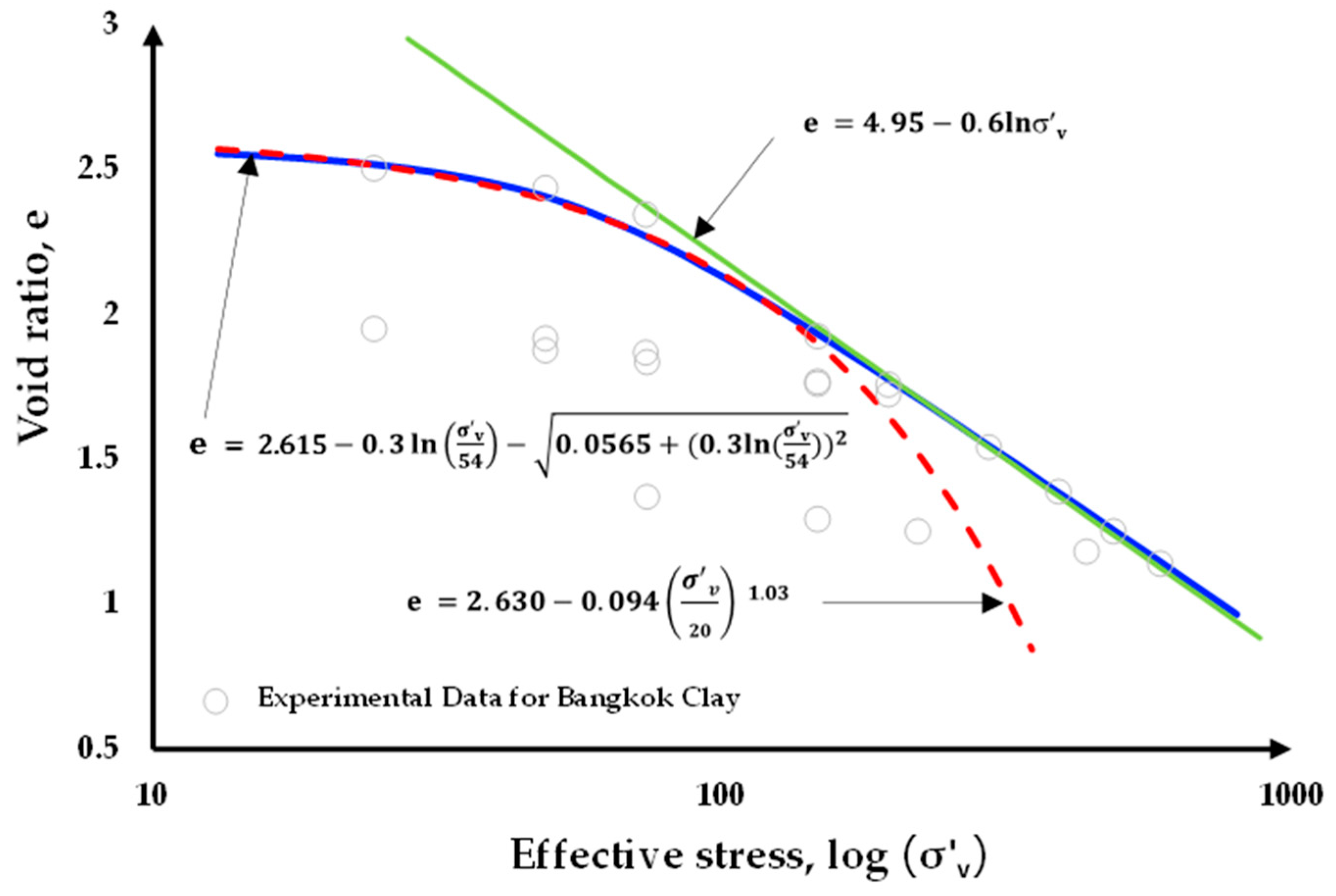
Figure 2.
Demonstration of the characteristics of the graphs for equation 6 with different parameters: (a) graphs varying parameter ; (b) graphs varying parameter ; (c) graphs varying parameter ; (d) graphs varying parameter .
Figure 2.
Demonstration of the characteristics of the graphs for equation 6 with different parameters: (a) graphs varying parameter ; (b) graphs varying parameter ; (c) graphs varying parameter ; (d) graphs varying parameter .
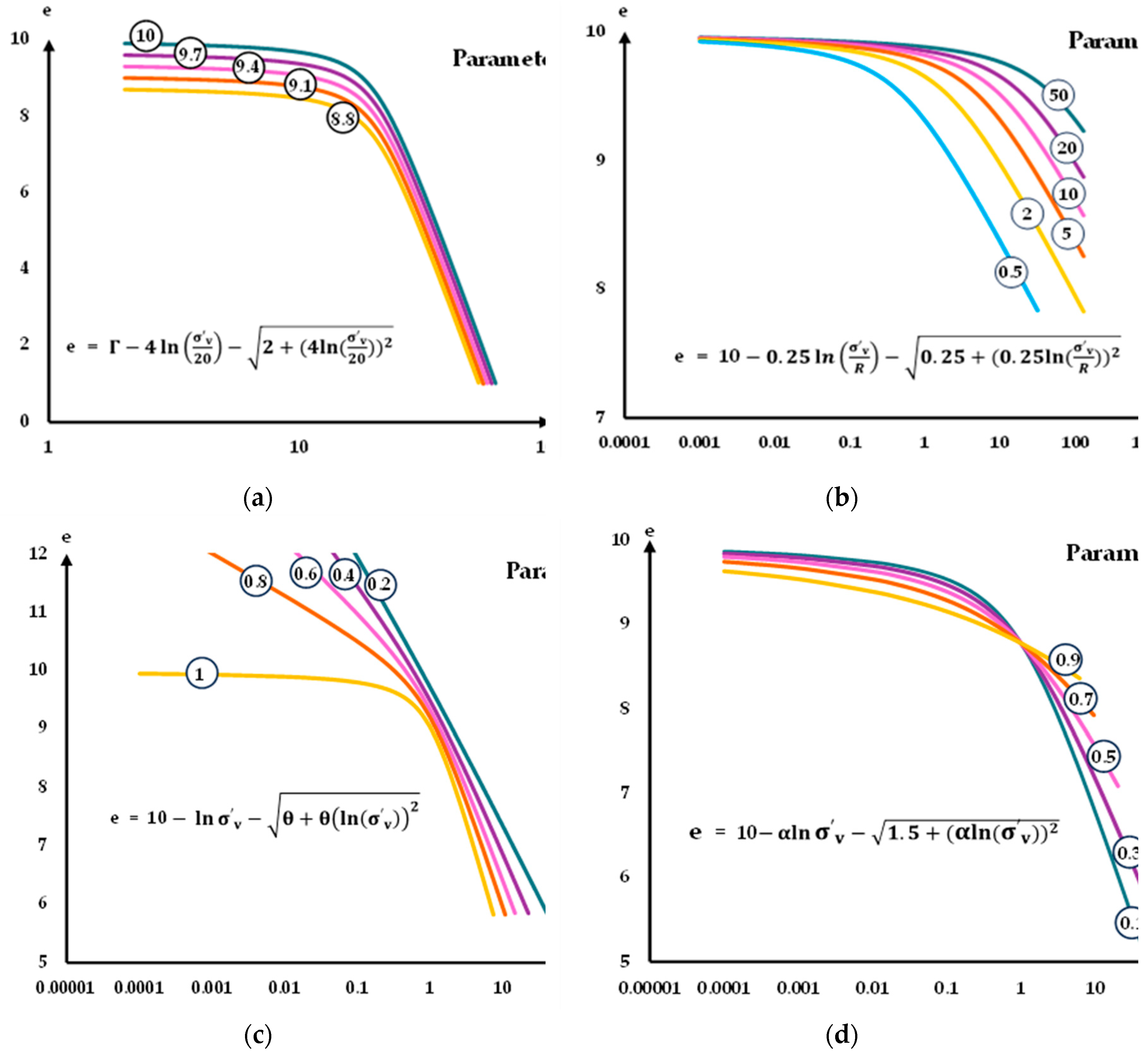
Figure 3.
Schematic of using parabolic equations for unloading and reloading lines.
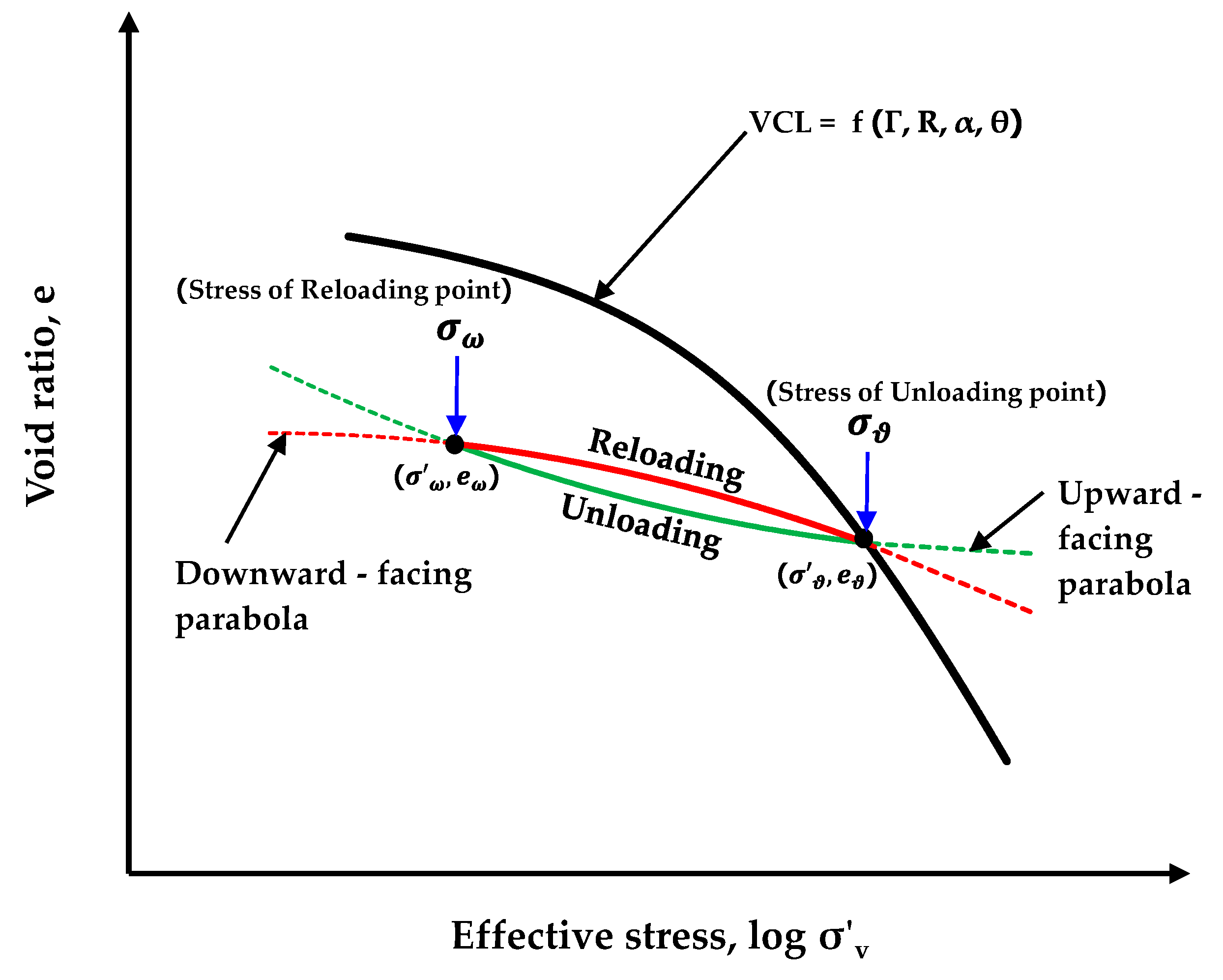
Figure 4.
Effect of parameter for the asymmetric hysteresis.
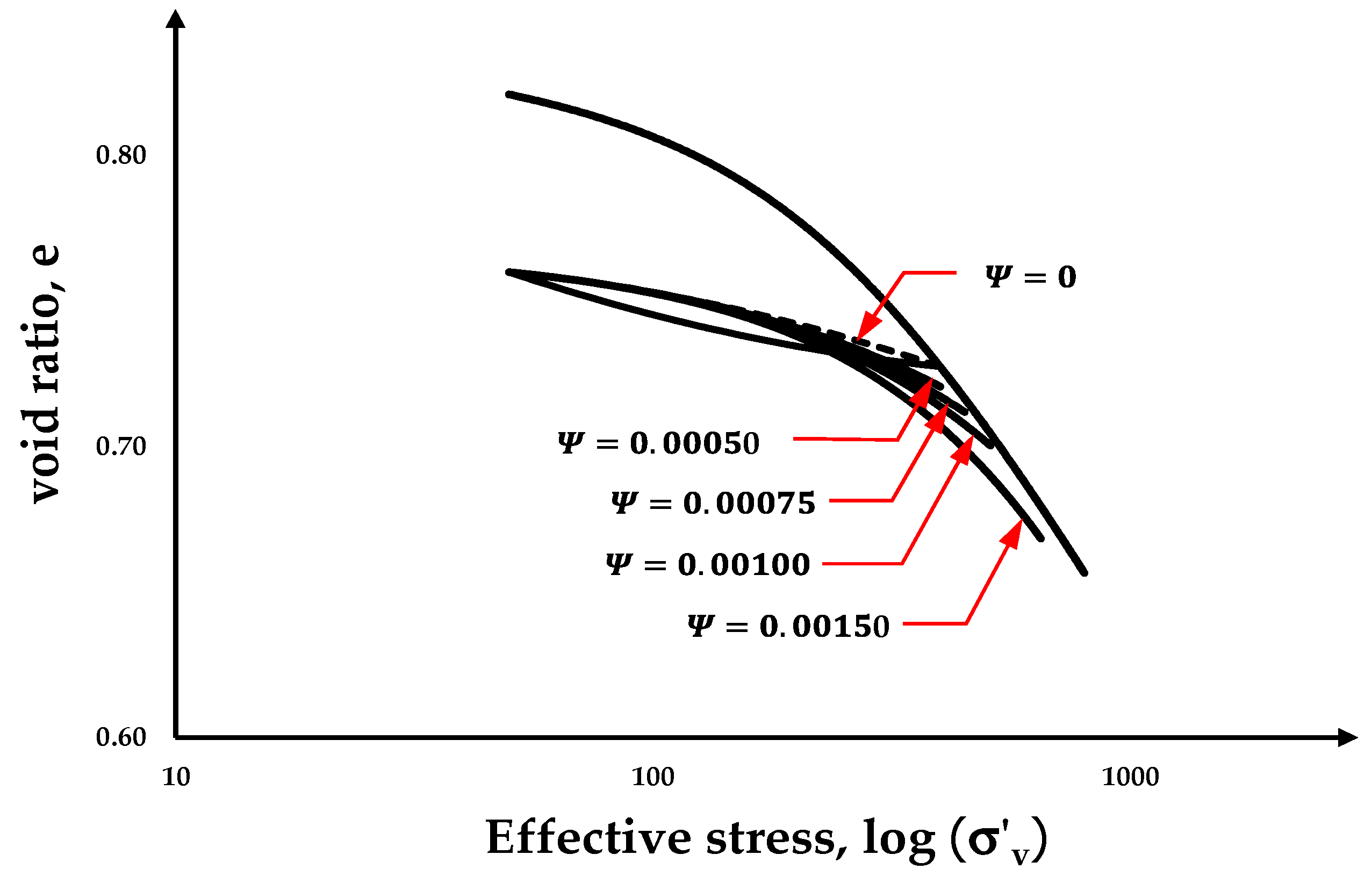
Figure 5.
Loading conditions for overconsolidated clays: (a) for ; (b) for .
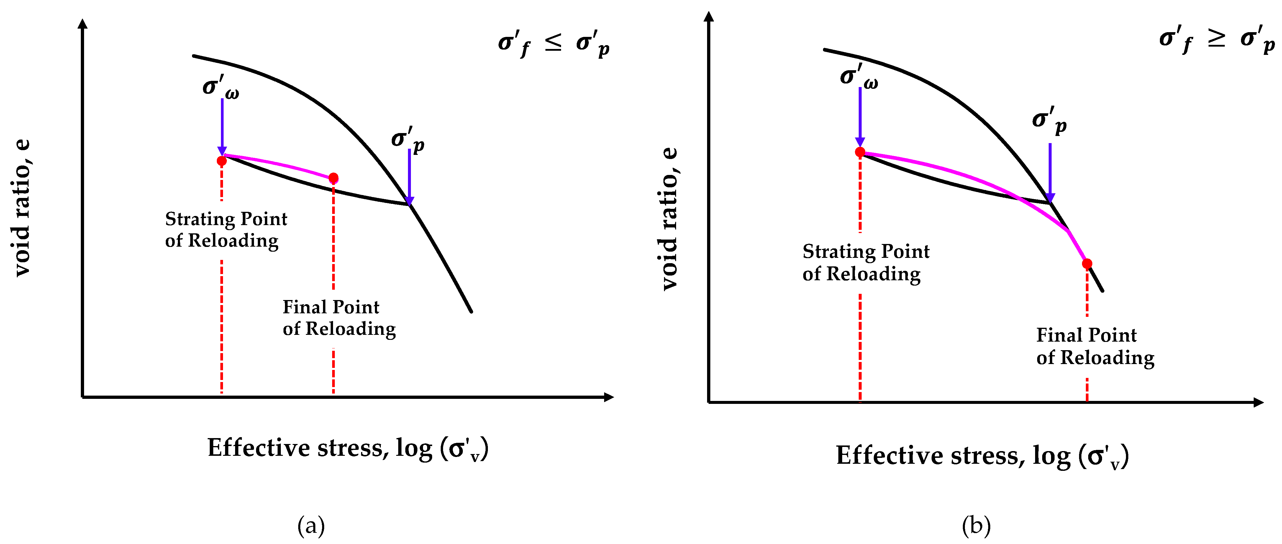
Figure 6.
Consolidation test data with best fit curves: Bangkok Clay.
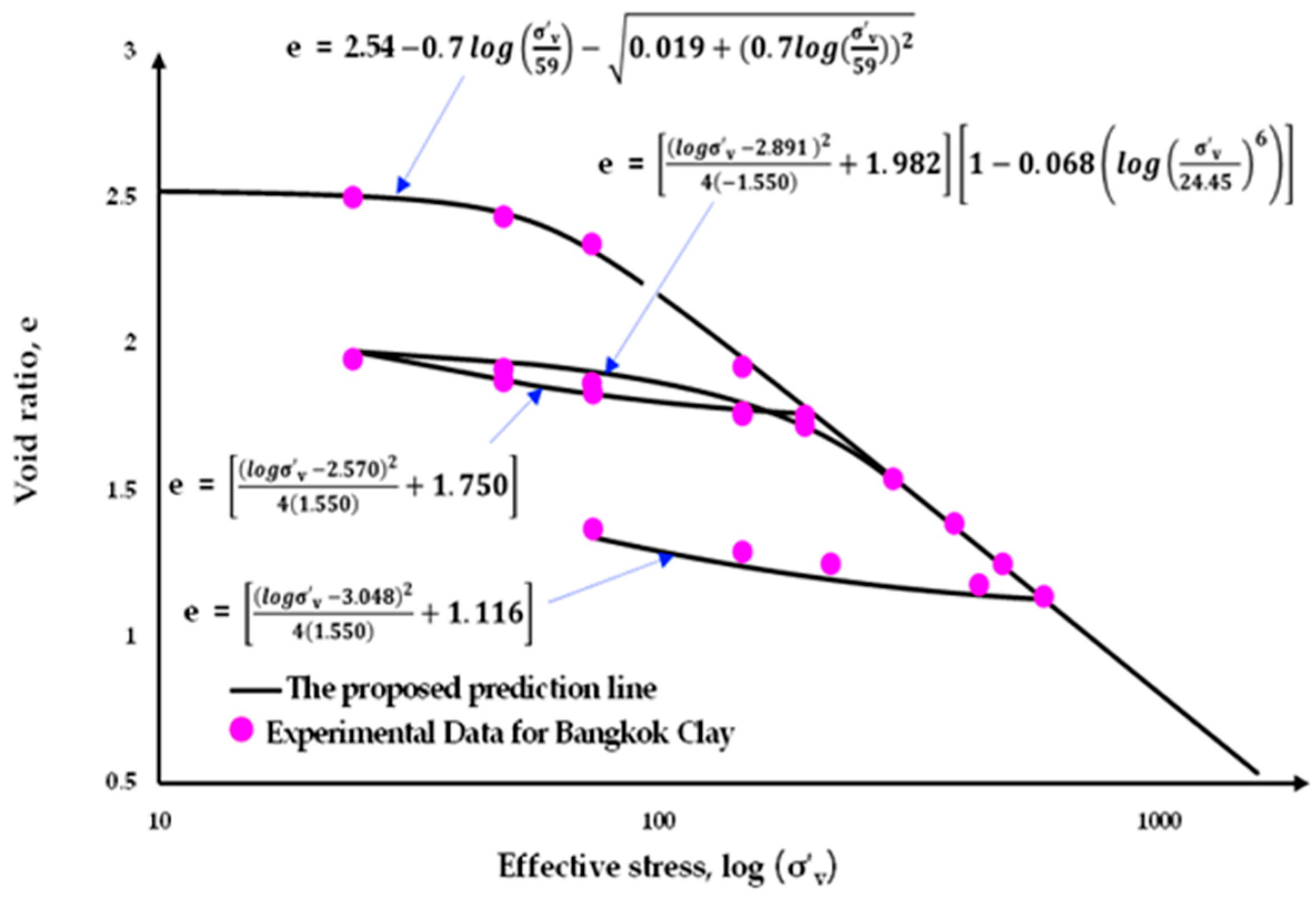
Figure 7.
Consolidation test data with best fit curves: Boston Blue Clay.
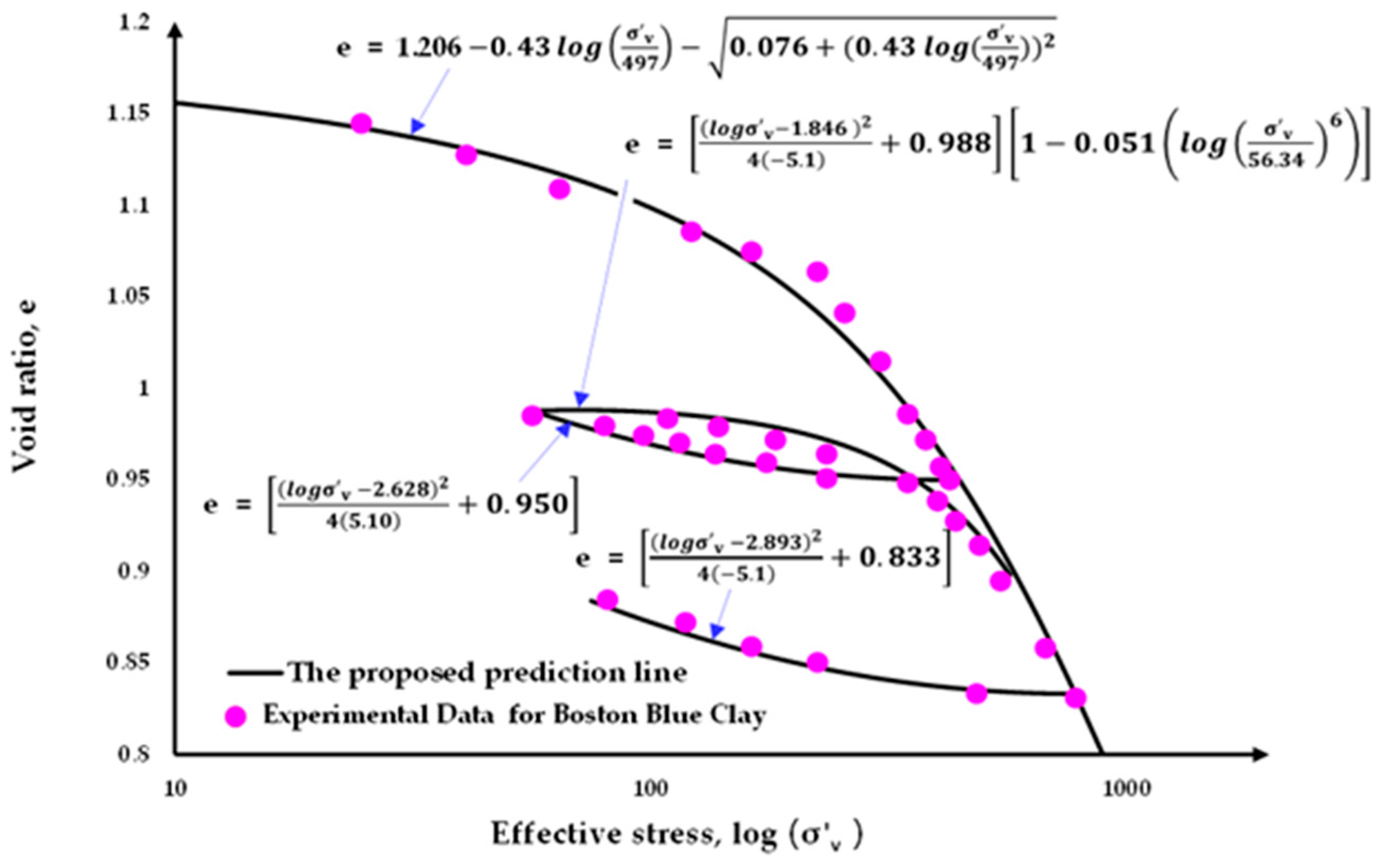
Figure 8.
Consolidation test data with best fit curves: London Clay.
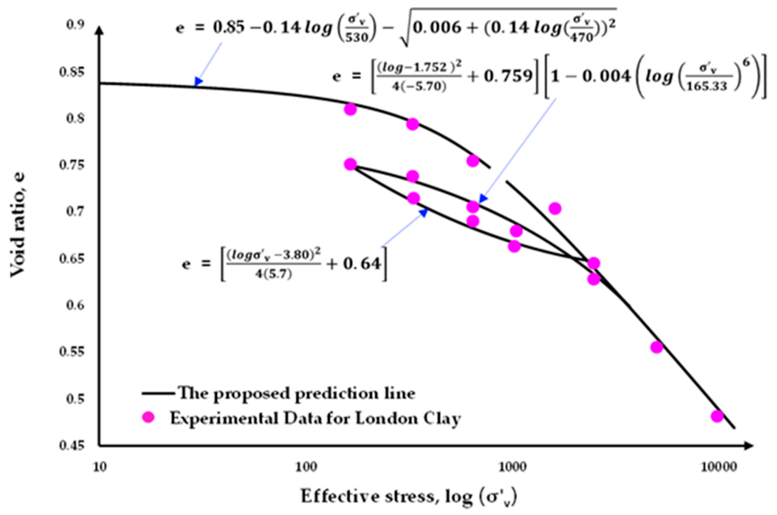
Figure 9.
Footing on clay to be used for consolidation settlement calculations: a) Single layer.
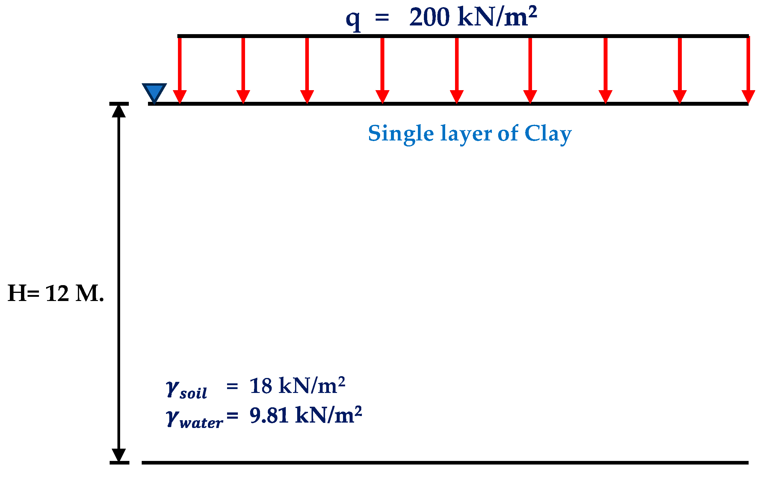
Figure 10.
Footing on clay to be used for consolidation settlement calculations: b) Equal thickness layers.
Figure 10.
Footing on clay to be used for consolidation settlement calculations: b) Equal thickness layers.
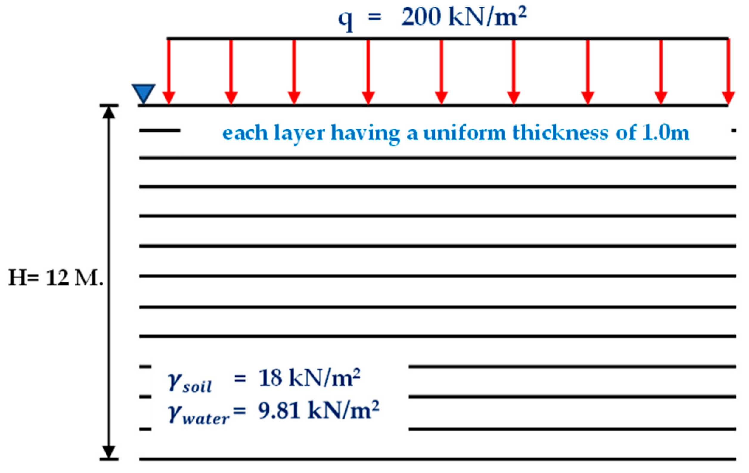
Figure 11.
Footing on clay to be used for consolidation settlement calculations: c) Varying thickness.
Figure 11.
Footing on clay to be used for consolidation settlement calculations: c) Varying thickness.
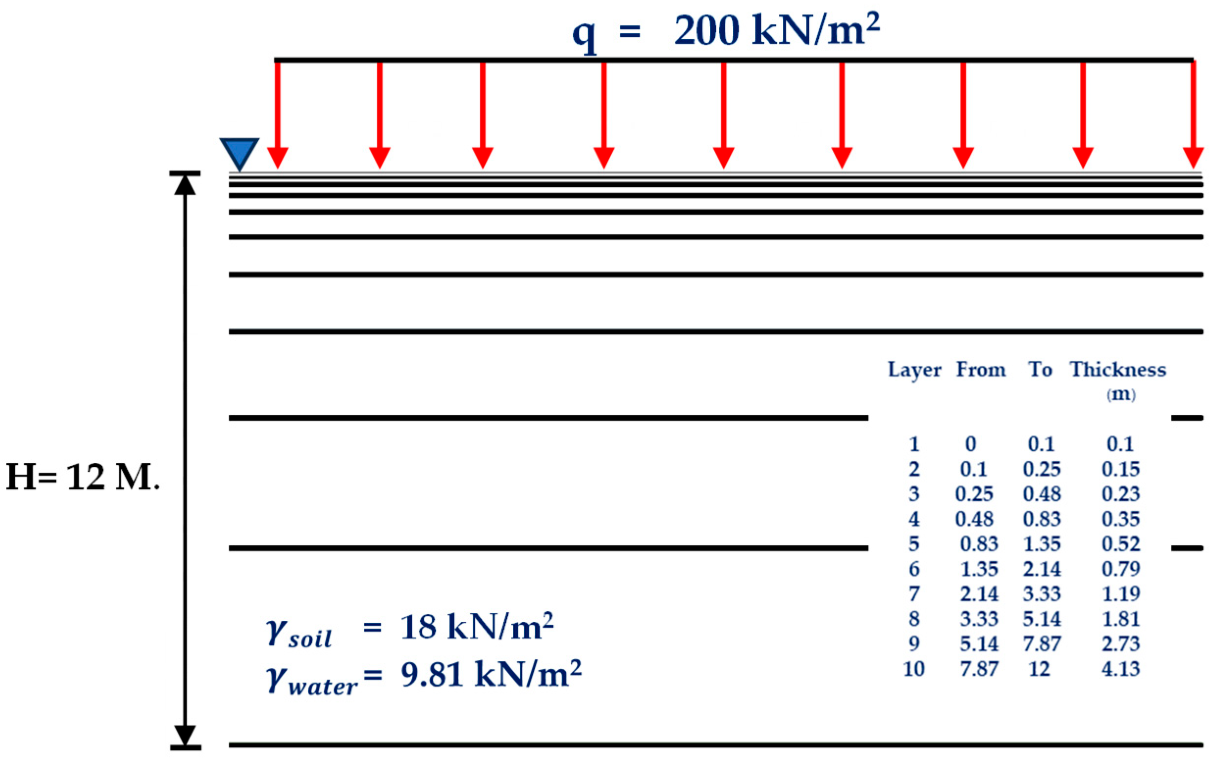

Table 1.
Soil parameters fitted from the laboratory test results.
| Type of soil | Virgin compassion line | Unloading – Reloading line | ||||||
|---|---|---|---|---|---|---|---|---|
| Boston blue clay | 1.206 | 0.430 | 497 | 0.076 | 5.10 | 2.628 | 0.950 | 0.051 |
| London clay | 0.850 | 0.135 | 530 | 0.0058 | 5.70 | 3.800 | 0.64 | 0.004 |
| Bangkok clay | 2.540 | 0.700 | 59 | 0.019 | 1.55 | 2.570 | 1.75 | 0.068 |
Table 2.
Comparison of total consolidation settlement of normally consolidated clay using LF, CF and AJOP methods for three soil data.
Table 2.
Comparison of total consolidation settlement of normally consolidated clay using LF, CF and AJOP methods for three soil data.
| Type of soil | Case | LF (Equation 3) |
CF (Equation 4) |
AJOP (Equation 6) |
|---|---|---|---|---|
| Boston Blue Clay | a) Single Layer | 1.566 | 0.302 | 0.284 |
| b) Equal Layer Thickness | 1.967 | 0.323 | 0.310 | |
| c) Varied Layer Thickness | 1.988 | 0.323 | 0.309 | |
| London Clay | a) Single Layer | 0.806 | 0.102 | 0.089 |
| b) Equal Layer Thickness | 1.012 | 0.109 | 0.097 | |
| c) Varied Layer Thickness | 1.023 | 0.108 | 0.097 | |
| Bangkok Clay | a) Single Layer | 2.334 | 3.453 | 1.832 |
| b) Equal Layer Thickness | 2.933 | 3.667 | 1.781 | |
| c) Varied Layer Thickness | 2.964 | 3.663 | 1.780 |
Table 3.
Comparison of total consolidation settlement for overconsolidated clay for low surface loading of 200 kN/m2.
Table 3.
Comparison of total consolidation settlement for overconsolidated clay for low surface loading of 200 kN/m2.
| Type of soil | Case | AJOP method (Equation 6) |
|---|---|---|
| Boston Blue Clay | a) Single Layer | 0.178 |
| b) Equal Layer Thickness | 0.207 | |
| c) Varied Layer Thickness | 0.205 | |
| London Clay | a) Single Layer | 0.072 |
| b) Equal Layer Thickness | 0.080 | |
| c) Varied Layer Thickness | 0.080 | |
| Bangkok Clay | a) Single Layer | 1.015 |
| b) Equal Layer Thickness | 1.119 | |
| c) Varied Layer Thickness | 1.101 |
Table 4.
Comparison of total consolidation settlement for overconsolidated clay for high surface loading of 1,000 kN/m2.
Table 4.
Comparison of total consolidation settlement for overconsolidated clay for high surface loading of 1,000 kN/m2.
| Type of soil | Case | AJOP (Equation 6) |
|---|---|---|
| Boston Blue Clay | a) Single Layer | 1.084 |
| b) Equal Layer Thickness | 1.139 | |
| c) Varied Layer Thickness | 1.138 | |
| London Clay | a) Single Layer | 0.397 |
| b) Equal Layer Thickness | 0.417 | |
| c) Varied Layer Thickness | 0.417 | |
| Bangkok Clay | a) Single Layer | 3.578 |
| b) Equal Layer Thickness | 3.659 | |
| c) Varied Layer Thickness | 3.651 |
Disclaimer/Publisher’s Note: The statements, opinions and data contained in all publications are solely those of the individual author(s) and contributor(s) and not of MDPI and/or the editor(s). MDPI and/or the editor(s) disclaim responsibility for any injury to people or property resulting from any ideas, methods, instructions or products referred to in the content. |
© 2025 by the authors. Licensee MDPI, Basel, Switzerland. This article is an open access article distributed under the terms and conditions of the Creative Commons Attribution (CC BY) license (http://creativecommons.org/licenses/by/4.0/).
Copyright: This open access article is published under a Creative Commons CC BY 4.0 license, which permit the free download, distribution, and reuse, provided that the author and preprint are cited in any reuse.


