
Submitted:
22 December 2025
Posted:
23 December 2025
You are already at the latest version
Abstract
Millimeter-wave (mmWave) detection is a widespread human activity recognition (HAR) method. However, due to the mmWave characteristics, it is challenging to per-form HAR in non-line-of-sight (NLOS) environments. Before the prevalence of artificial intelligence (AI) technologies, mmWave-based HAR systems mainly relied on tradi-tional signal processing and handcrafted feature extraction (e.g. time–frequency analy-sis, multi-path modeling, micro-Doppler signature analysis), combined with classical classifiers such as Support Vector Machine (SVM) or Random Forest. However, these approaches were highly sensitive to environmental variations and failed to generalize in NLOS conditions. With the advent of AI, techniques such as Convolutional Neural Network (CNN) have played a crucial role in feature extraction from two-dimensional images generated by mmWave radar signals. In this paper, for the first time, a frame-work for Federated Continual Learning (FCL) based on CNN is proposed for improving radar detection accuracy in NLOS environments while preserving personal privacy through local training without uploading radar tensors and personal data to the global server for model aggregation. Additionally, the FCL model learns from both LOS and NLOS environments for improving cross-domain adaptability and recognition.
Keywords:
federated continual learning
; millimeter-wave
; human activity recognition
; line-of-sight
; non-line-of-sight
; domain shift
; convolutional neural network
; catastrophic forgetting
; domain generalization
1. Introduction
Human activity recognition (HAR) has become a fundamental component in many intelligent systems, including smart homes, healthcare monitoring, human–computer interaction, and safety monitoring. Nowadays, chip-integrated millimeter-wave (mmWave) radar sensors are popular in many applications. When networked for an application such as HAR, these sensors can be considered as Internet-of-Things (IoT) devices, and the HAR can be seen as an IoT-based system. Compared to traditional vision-based sensing, mmWave radar sensors provide better privacy protection and exhibit strong adaptability to diverse environmental conditions [1]. The operating frequency range of mmWave radar, between 30 and 300 GHz, enables the capture of fine-grained motion patterns by analyzing reflected electromagnetic signals. These advantages make mmWave radar one of the best choices for non-invasive and contactless HAR systems [2].
In mmWave radar, Frequency-Modulated Continuous-Wave (FMCW) frames are converted into single-channel two-dimensional (2D) tensors such as range– or micro-Doppler, which serve as image-like inputs while avoiding identity-revealing appearance. On the other hand, machine learning techniques such as Federated Learning (FL) where each client holds disjoint data shards and only transmits model updates to the server without sharing raw radar frames, ensure data privacy. Aggregation uses Federated Averaging (FedAvg) to approximate on-device learning under privacy constraints.
Traditional mmWave-based HAR methods rely on handcrafted features and classical machine learning classifiers such as Support Vector Machine (SVM), k-Nearest Neighbors (kNN), and Random Forest [3]. In those methods, radar signals must be converted into range–Doppler maps or micro-Doppler spectrograms, from which features such as signal energy and Doppler shifts are manually extracted and input into SVM or kNN. Although traditional methods perform well in ideal environments, they are easily affected by noise, reflected signals, and target direction changes. In particular, under non-line-of-sight (NLOS) conditions, radar signals are strongly influenced by obstacles, leading to diffraction, scattering, and refraction effects that distort the received signal. Therefore, traditional mmWave-based radar detection in HAR is challenging to generalize across different environments and conditions. Physically, NLOS induces path distortions, such as diffraction around corners, multi-bounce scattering, partial occlusions, and energy attenuation that smear micro-Doppler ridges and alter class-specific patterns [4]. This physics-driven distortion explains why feature calibrations optimized for line-of-sight (LOS) scenarios can become unstable across sites, subjects, and layouts.
Artificial Intelligence (AI) has brought a significant breakthrough in the field of radar-based detection. Techniques such as Convolutional Neural Networks (CNNs) can automatically learn key spatial representations that distinguish different actions or targets from two-dimensional radar-derived images such as range–Doppler maps or micro-Doppler spectra, without manual feature engineering [5,6]. The CNN model converts the signals collected by the radar into a heat map, resembling an image. The horizontal axis represents the distance or angle of the person from the radar, while the vertical axis represents the speed of movement or the change in range. By analyzing local patterns in these images, such as the trajectory of arm swings and the energy distribution of body movement, the model can automatically determine a person's movements, thereby achieving accurate and stable human behavior recognition [7]. Nevertheless, CNN-based models are typically trained on data collected under controlled LOS conditions and tend to overfit the environment-specific channel characteristics. As a result, models trained in one domain (i.e. LOS) often fail to generalize to unseen NLOS scenarios [8]. Our preliminary studies show that standalone CNNs can achieve good performance under LOS conditions but their accuracy drops significantly in cross-domain (LOS−NLOS) recognition, as they are sensitive to phase order and perturbation intensity in cross-phase and cross-intensity NLOS, limiting cross-domain stability. This observation is consistent with the limited generalization caused by domain transfer [10]. At the same time, under staged or continual training, the model experiences catastrophic forgetting when adapting to subsequent phases, limiting stability and memory retention.
Addressing this domain generalization problem in mmWave-based HAR is challenging because it involves two intertwined issues: (i) domain shift between LOS and NLOS signal distributions, and (ii) catastrophic forgetting when adapting models to new environments over time. Simply fine-tuning CNNs on NLOS data may improve recognition in that domain but often leads to severe degradation of previously learned LOS knowledge, making the model unstable and unreliable for sustainable deployment. Moreover, collecting large-scale labeled NLOS data for each new environment is time-consuming and impractical.
To address these limitations, this paper proposes a Federated Continual Learning (FCL) framework, which enables stable mmWave HAR adaptation between LOS and NLOS conditions. The FCL paradigm combines the strengths of Federated Learning and Continual Learning, namely distributed learning across heterogeneous clients and long-term knowledge retention. To improve adaptation stability, we formalize the progressive LOS-to-NLOS domain shift in HAR as a FCL problem, where each NLOS severity level is treated as a sequential domain in a continual adaptation process. The local radar clients perform sequential task learning (e.g. from LOS to NLOS) and model updates are periodically aggregated on the global server without sharing raw data, thus balancing privacy and generalization.
The framework integrates selective layer freezing with L2 Starting Point (L2-SP) regularization under a three-phase training with increasing NLOS severity, which are light, medium, and hard. At the beginning of each phase, early layers, including the stem and the first residual block, are frozen to preserve low-level spectral–temporal features. Meanwhile, L2-SP regularization constrains the trainable parameters toward those of the previous phase, reducing destructive parameter drift. Knowledge distillation (KD) from the previous phase can be applied as an auxiliary stabilizer while learning NLOS-specific features, or disabled to maintain a lightweight and consistent training setting.
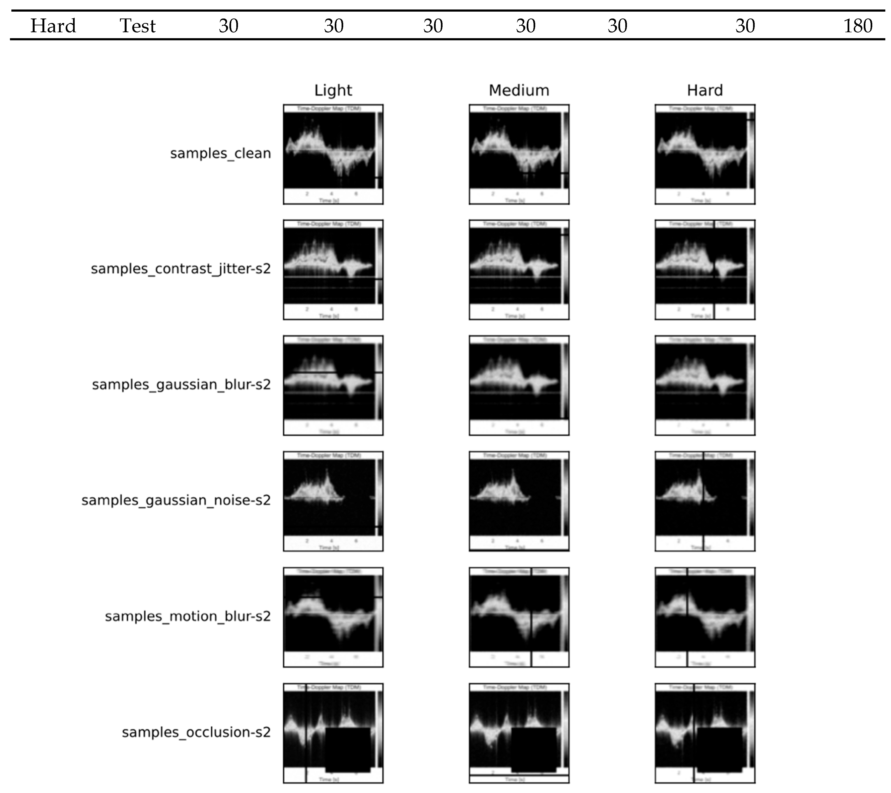
In addition to the core FCL-based framework, we explore strategies to further improve cross-domain adaptability and recognition in NLOS environments by (i) performing warm-up training on fully connected layers in the new domain; and (ii) gradually unfreezing selected backbone blocks for controlled adaptation. To obtain NLOS characteristics (e.g. reduced signal-to-noise ratio (SNR), energy dispersion, and limited visibility) without site-specific data collection, we construct NLOS datasets from LOS tensors via controlled, physically motivated perturbations [9], including additive noise that reduces SNR, multiplicative speckle, anisotropic blur, band and block dropouts, tile-wise occlusion, and low-frequency clutter.
The rest of the paper is organized as follows. Section 2 reviews related work. Section 3 formulates the mmWave HAR problem. Section 4 details the NLOS construction and evaluation protocol. Section 5 presents the proposed framework. Section 6 analyzes and discusses the results. Finally, Section 7 concludes the paper with some directions for future work.
2. Related Work
2.1. mmWave HAR: Conventional vs. Deep Learning Approaches
Early mmWave HAR used handcrafted features and simple models. Researchers first converted radar data into range– or micro-Doppler maps and then extracted features like Doppler center, bandwidth, or energy pattern. These features were given to models such as SVM and kNN, which worked well when radar had a clear LOS, but failed even when the features shifted only slightly due to small environmental or subject positional changes. Deep learning, particularly CNNs, removes the need for such handcrafted features by learning useful spatial and temporal patterns directly from radar data [11]. This makes CNNs more flexible and better for complex environments with reflections and occlusions.
2.2. Domain Generalization and Adaptation under NLOS Conditions
Domain adaptation and generalization help reduce accuracy drops when data from training and testing come from different environments. Standard methods include matching features across domains, using adversarial training, or changing data styles. However, these methods often need large and balanced datasets with labelled samples from both domains (e.g. LOS and NLOS), which radar typically does not have. Additionally, radar spectrograms follow physical rules so that even simple feature alignment may damage the motion information inside Doppler patterns [12].
Alternatively, NLOS datasets can be constructed from perturbing LOS datasets with physical effects such as reduced signal strength, blurring and cluttering to simulate real radar effects. This approach removes the need to collect real NLOS data and preserves the original link between signal loss and radar reflection [8].
2.3. Federated and Continual Learning for mmWave HAR
Federated learning allows the models to train across many devices without sharing raw data, which protects user privacy [13]. Continual learning helps models keep past knowledge when new tasks arrive. Most existing FCL studies primarily focus on image or speech domains, where data are typically high-dimensional and relatively homogeneous across clients [14]. In contrast, radar-based HAR presents a more challenging setting, as datasets are often small-scale, device-dependent, and sensitive to variations in physical deployment and environmental conditions.
Early CNN layers are fixed to protect low-level range–Doppler patterns, and higher layers are updated to learn new conditions. Tests show that this design reduces forgetting, keeps performance stable across training phases, and lowers task-order effects measured by Average Forgetting (AF) and Backward Transfer (BWT) [15].
These findings from the literature motivated us to bring together, for the first time, federated and continual learning in a physics-aware and privacy-preserving radar system for robust HAR under domain shifts.
3. Problem Formulation
3.1. Task Setup and Sequential Domain Definition
Building on the above motivation, we formalize the mmWave HAR task under sequential domain shifts from LOS to NLOS within a privacy-constrained federated setting. Let the learning schedule consist of three phases that correspond to increasing perturbation severities: light, medium and hard. At phase , the dataset is , where is a single-channel 2D tensor derived from FMCW radar information such as range– Doppler or micro-Doppler, and denotes the activity class. The classifier produces and is updated sequentially across phases.
3.2. Privacy Constraint and Federated Setting
In realistic deployments, radar tensors remain on local devices due to privacy and governance considerations. Consequently, training follows a federated paradigm with K clients. Each client holds a disjoint shard of and performs local updates without sharing raw tensors. A central server aggregates model parameters or updates at the end of each round using sample-size-weighted averaging (FedAvg). This constraint shapes both the algorithmic design and evaluation protocol by ruling out methods that require centralised access to the full dataset or inter-client raw data exchange [16].
3.3. Sequential Objective and Retention Challenges
The training objective combines plasticity, the ability to adapt to the current phase’s distribution and stability, and the ability to retain competencies learned in earlier phases. Let be the consolidated parameters after completing phase . At the beginning of phase , the consolidated model serves as the reference for continued adaptation. A central challenge is to avoid catastrophic forgetting, i.e. a deterioration of performance on earlier phases (Light/Medium) when updating for the hard phase. In this setting, high peak accuracy at an intermediate phase is not sufficient; what matters operationally is the terminal model and its cross-phase behavior.
3.4. Formal Training Objective
Local training at phase minimizes a supervised loss on augmented with a soft parameter regularizer that discourages large drifts from a reference (chosen as ):
where
- is instantiated as L2-SP with , softly constraining drift from previous consolidated model, and is the merging parameter for phase ;
- is the dataset of phase ;
- denotes an mmWave radar tensor and its activity label;
- is the consolidated model after completing phase;
- is the reference model anchoring the update for phase ;
- denotes the supervised task loss (cross-entropy);
- is the L2-SP regularization coefficient;
- softly constrains parameter drift from previous consolidated model.
3.5. Cross-Phase Evaluation Protocol
After each phase, the server snapshot (After-P1, After-P2, After-P3) is evaluated on all three severities, producing a cross-phase accuracy matrix . The corresponding AF and BWT [17] are computed as:
where
- is the performance on severity s after completing training up to phase p;
- is the performance evaluated on severity s immediately after completing training on severity s;
- is the performance on severity s using the final model after completing all P phases;
- is the number of sequential phases (here : Light, Medium, Hard);
- is the number of severity levels (here S = P = 3)
- is forgetting for severity s;
- AF quantifies terminal retention loss;
- BWT indicates whether final adaptation benefits earlier domains.
4. NLOS Construction and Evaluation Protocol
4.1. Data Representation and Preprocessing
Radar frames are represented as single-channel, image-like tensors derived from range– or micro-Doppler maps. Each sample is stored or converted to (channel-first), which avoids identity-revealing appearance cues and aligns with the sensing physics. Per-sample min–max normalization to [0,1] is applied:
where
- is raw radar tensor;
- is normalized tensor;
- min, max denote sample-level minimum and maximum, respectively;
- is numerical stabilizer
All input samples are resized to 224×224 using bilinear interpolation implemented via OpenCV (INTER_LINEAR), ensuring compatibility with the ResNet-18 backbone. If a file is multi-channel, such as RGB or stacked features, channels are averaged to obtain a single-channel intensity map prior to normalization:
where
- C is number of channels;
- is channel c;
- is collapsed single-channel tensor.
Arrays already in are preserved. The same directory hierarchy is consistently applied across all experimental phases (light, medium, and hard), thereby ensuring alignment of label indices and comparability of results across domains. Perturbation severities and corresponding seeds are provided in Section 4.2, and dataset split statistics are summarized in Section 4.3 (Table 2 and Table 3).
4.2. NLOS Perturbation Pipeline – Evaluation Settings
To approximate dominant NLOS effects without relying on site-specific recordings, a deterministic perturbation pipeline is applied at evaluation time. The transformations include additive white Gaussian noise for SNR degradation, multiplicative speckle for coherent interference, anisotropic Gaussian blur for Doppler and range smearing, frequency-selective band dropouts for shadowing and fading, tile-wise occlusion for partial observability, and contrast jitter for slow-varying clutter. The composite perturbation is expressed in (8), followed by contrast adjustment in (9):
where
- is clean radar tensor;
- is perturbed tensor after NLOS pipeline;
- is additive Gaussian noise;
- is multiplicative speckle noise;
- is anisotropic Gaussian blur with kernel widths ;
- is frequency band-dropout mask;
- is tile-wise occlusion mask;
- = elementwise multiplication;
- = contrast jitter coefficient;
Evaluation severities are generated with fixed seeds for reproducibility, whereas training employs stronger randomized augmentation to promote robustness under distribution shifts.

Table 1.
NLOS parameter settings for different severity levels.
| Severity | AWGN | Speckle | Blur | Band dropout probability | Occlusion probability | Contrast jitter |
|---|---|---|---|---|---|---|
| Light | 0.020 | 0.020 | (3, 1) | 0.03 | 0.02 | 0.05 |
| Medium | 0.040 | 0.040 | (5, 3) | 0.05 | 0.04 | 0.08 |
| Hard | 0.060 | 0.060 | (7, 5) | 0.08 | 0.06 | 0.12 |
* Seeds: Validation/Test use a fixed evaluation seed (e.g., 42) for reproducibility. * Parameter settings in the table are designed by authors to approximate key NLOS degradations.
To make results easy to reproduce, the Light, Medium, and Hard setting in this paper use fixed parameter ranges:
- Additive noise (AWGN) has SNR values of 20–25 dB for Light, 15–20 dB for Medium, and 10–15 dB for Hard.
- Anisotropic Gaussian blur uses
- Tile occlusion covers 5 %, 10 %, and 15 % of the image tiles.
- Contrast changes by ±10 %, and band-dropout rates follow Table 1.
Random noise and perturbations are applied to each batch during training to improve generalization. Fixed random seeds are used for validation and testing, so that the results are consistent. This design ensures that any performance change across phases comes from the model’s adaptability, not random variation.
The perturbation parameter settings are set to approximate real mmWave propagation characteristics such as diffraction, multipath scattering, and signal attenuation [9]. This ensures the NLOS conditions serve as a realistic proxy for actual through-wall or occluded scenarios, minimizing the simulation-to-real-world gap in the evaluation protocol.
4.3. Data Splits and Counts
Datasets are split into 70/15/15 proportions corresponding to training/validation/testing. Each stage produces 840, 180, and 180 samples, respectively, due to six activity classes. Thus, each training class has 140 samples, while each class of validation and testing has 30 samples. Because NLOS for evaluation is generated on the fly, the Light, Medium, and Hard phases share the same split counts as the LOS setting.
To simulate NLOS conditions, a physics-inspired perturbation stack is applied to the original LOS radar data. The NLOS pipeline adds several types of signal changes, including Gaussian noise, speckle noise, blur along the Doppler and range directions, frequency-band dropouts, tile-wise occlusion, and low-frequency contrast jitter. Three severity levels, Light, Medium, and Hard, are used to control the strength of these perturbations and to evaluate model robustness under different levels of domain shift.
Table 2.
Phase-wise sample counts per split.
| Phase | Train | Validate | Test | Total |
|---|---|---|---|---|
| Light | 840 | 180 | 180 | 1200 |
| Medium | 840 | 180 | 180 | 1200 |
| Hard | 840 | 180 | 180 | 1200 |
* LOS radar data used in this work are obtained from a publicly available mmWave HAR dataset [20], while all NLOS data are generated by the authors.
Table 3.
Class counts per phase and split (example with six classes).
| Phase | Split | Falling to waving for help | Sitting down to drinking water | Sitting down to stretching | Sitting down to walking | Walking to Falling | Walking to falling, Walking to picking up things | Total |
|---|---|---|---|---|---|---|---|---|
| Light | Train | 140 | 140 | 140 | 140 | 140 | 140 | 840 |
| Light | Validate | 30 | 30 | 30 | 30 | 30 | 30 | 180 |
| Light | Test | 30 | 30 | 30 | 30 | 30 | 30 | 180 |
| Medium | Train | 140 | 140 | 140 | 140 | 140 | 140 | 840 |
| Medium | Validate | 30 | 30 | 30 | 30 | 30 | 30 | 180 |
| Medium | Test | 30 | 30 | 30 | 30 | 30 | 30 | 180 |
| Hard | Train | 140 | 140 | 140 | 140 | 140 | 140 | 840 |
| Hard | Validate | 30 | 30 | 30 | 30 | 30 | 30 | 180 |
| Hard | Test | 30 | 30 | 30 | 30 | 30 | 30 | 180 |
Figure 1.
NLOS exemplars across severity levels (light, medium, hard).
Randomness in Training and Evaluation: Training uses stochastic perturbations to enhance robustness; validation and testing use milder, reproducible settings with fixed seeds. This separation ensures that cross-phase differences reflect model behavior rather than randomness in distortions.
Splits and Federated Partitioning: For each severity, disjoint training, validation, and testing splits are used. Only the training split is distributed across clients, while the validation and testing sets remain centralized to ensure consistent evaluation of the server snapshots.
Three-Phase Schedule and Matrices: The training schedule progresses from Light to Medium to Hard. After each phase, the consolidated model is saved and evaluated across all severity levels, producing matrices that enable the computation of AF and BWT. Unless otherwise stated, models are trained on the NLOS training set, tuned on the NLOS validation set, and evaluated on the NLOS testing set, with Medium serving as the default testing condition.
4.4. Federated Partition and Training Protocol
Data are distributed over clients (client 01 to client 03) with class-balanced shards; each client participates in every communication round (participation ratio = 1.0). Training follows a standard FedAvg schedule with rounds per phase. Each client performs local epoch per round using AdamW with batch size = 64, learning rate = and weight decay . Unless otherwise stated, all phases use the same optimiser and learning-rate setting. Model aggregation on the server uses FedAvg without momentum; raw radar tensors remain on the device, and only model updates are transmitted.
At the beginning of each new phase (light, medium, hard), the low-level feature extractor is warm-started and partially frozen to preserve previously acquired spectral–temporal primitives: specifically, stem and layer1 are frozen, while deeper layers remain trainable. To limit destructive drift, an L2-SP penalty is applied to the trainable parameters with coefficient anchoring them to the consolidated weights from the previous phase. The main configuration does not use KD. For completeness, ablations with KD employ a fixed teacher equal to the previous-phase checkpoint, temperature , and distillation weight . This recipe yields stable cross-phase performance while maintaining adaptation capacity under increasing NLOS severity.
Each phase concludes with model consolidation on the server and centralized validation of the global snapshot. Validation accuracy and macro-F1 are recorded after every federated round. The best model from each phase is checkpointed for later cross-phase evaluation. All subsequent AF and BWT calculations and heatmaps in Section 5 are derived from these checkpoints. This unified protocol ensures that every reported result corresponds to a deterministic run with seed = 42, allowing exact reproduction on comparable hardware setups.
4.5. Evaluation Protocol
Unless otherwise specified, models are trained on the NLOS training split, tuned by early stopping on the validation split, and all results are reported on the test split. Validation/test severities and random seeds follow Table 1; split statistics follow Table 2 and Table 3. The best-validation checkpoint is restored prior to final testing.
Model selection uses macro-F1 on the validation split with patience = 5 evaluation steps. Unless noted otherwise, a fixed seed = 42 is used for the main runs; variability in ablations is summarized as mean ± standard deviation over three seeds {0, 1, 2}. Primary metrics are:
- Overall Accuracy (ACC): fraction of correctly classified samples.
- Macro-F1: unweighted mean of per-class F1 scores (mitigates skew from class imbalance).
- Diagnostics: per-class scores and confusion matrices are reported when informative.
Per-class scores and confusion matrices are reported where informative. AF and BWT as defined in Section 3.5 are computed under the fixed-severity protocol in Table 1, with the same random seeds and splits in Table 2 and Table 3. The performance metric (ACC or macro-F1) for cross-phase accuracy matrix as defined in Section 3.5 is kept consistent for all entries.
Under the evaluation protocol in this section and the fixed severities and seeds defined in Table 1, the FCL configuration attains and , indicating negligible forgetting with slightly positive backward transfer. The CNN-only sequential baseline yields and . The corresponding cross-phase validation accuracy matrix A for the CNN baseline is shown in Table 4.
5. Proposed Framework
5.1. Overview
In this section, the proposed FCL framework for mmWave HAR is introduced which targets scenarios under sequential domain shifts from LOS to NLOS. This method instantiates a practical training loop that: (i) protects privacy by exchanging only model updates; (ii) maintains the learned representation of the model at each stage effectively through warm-start parameter freezing and L2-SP regularization mechanism; and (iii) is equipped with switchable lightweight KD for stable adaptation.
5.2. FCL Formulation
Let the training process consist of three sequential phases , corresponding to light, medium, and hard NLOS severities. At phase , each client holds a local dataset and trains a model with parameters , where denotes the trainable parameters of the global model. A global server aggregates local updates via FedAvg, without accessing raw radar tensors.
Continual adaptation is implemented by initializing phase from the best checkpoint of phase , denoted (with denoting the randomly initialized or pretrained weights). A layer-freezing mask indicates the parameters to remain frozen, such as the early convolutional blocks, while represents the complementary trainable subset. The objective at a client is:
where is cross-entropy; is softmax function; is a fixed teacher snapshot (the phase p−1 model); is the softmax temperature in KD; and are weights for the L2-SP regularization term, and KD loss, respectively ( is set to when KD is not used); KL denotes the Kullback–Leibler divergence; L2-SP is always active on unfrozen layers; element-wise mask that enforces warm-start freezing parameters with is kept fixed; and only is updated.
After local epochs on each participating client, the server aggregates by:
where is the set of sampled clients in the round and . Across rounds, validation on the phase held-out set selects the best checkpoint. Cross-phase validation matrices evaluated on phase-1, 2, and 3 validation sets are computed after each phase to quantify stability, and the AF and BWT are then computed as given in Section 3.5.
5.3. Backbone and Input Processing
A ResNet-18 backbone is adapted to single-channel radar tensors. The first convolution is modified from 3 to 1 input channel with 64 output channels: the final fully connected (FC) layer maps to the number of activity classes (six in the experiments). Input frames are grayscale tensors stored as either or ; preprocessing normalizes all inputs to [0,1], reshapes to , and resizes to 1×224×224 before feeding the network. This keeps the convolutional stem unchanged apart from the input channel count, preserving the inductive bias of ResNet-18 while matching the mmWave spectrogram-like inputs.
5.4. Objectives and Regularization
Cross-entropy on per-frame logits is used throughout. L2-SP softly constrains trainable parameters to remain close to their previous-phase optima on unfrozen layers, counteracting representational drift that otherwise causes forgetting. In contrast to full parameter freezing, which can lead to underfitting in new phases, L2-SP allows controlled movement toward the new domain while penalizing unnecessary deviation [18].
When enabled, KD supplies a soft target from the phase teacher, stabilizing decision boundaries that were reliable in earlier phases. KD is lightweight in computation and used as a knob; and ablations adjust .
Early convolutional blocks are frozen at the beginning of each new phase; later blocks and the classifier head are updated. This provides: (i) strong low-level priors for range–Doppler structures; and (ii) the capacity to adapt high-level class separation to NLOS distortions. The freezing depth is fixed per experiment and varied only in ablations.
5.5. Training Schedule Across Phases
Each stage proceeds rounds of FedAvg. In round , each selected client trains for local epochs with Adam with Decoupled Weight Decay (AdamW) using learning rate , weight decay and batch size . The training starts with the global weight of broadcasting. After aggregation, the server validates on the current phase’s validation set, and the best-validation checkpoint across the rounds is saved as . Immediately upon finishing phase , cross-phase validation is performed with on all three-phase validation sets and recorded as the -th row of the cross-phase matrix. These snapshots are also used later for test-set evaluation in Section 6.
The simulation experiments use three training phases (light, medium, and hard), the same backbone and preprocessing for all phases, AdamW with , , , and short local epochs per round to respect GPU constraints while still exposing the model to federated variability. L2-SP is active in all experiments, and KD is optional.
5.6. Federated Protocol and Partitioning
A simulated federated environment is adopted to approximate on-device training. The client data are class-balanced per share to decouple order-sensitivity from extreme non–independent and identically distributed (non-IID) effects; client participation is full in each round. This setting isolates the phenomena of interest: domain shift and forgetting, without confounding from intermittent client availability or severe label skew [16].
5.7. Algorithm
The detailed steps of the proposed FCL framework with warm-start freezing, L2-SP, and optional KD, are shown in .
| Algorithm 1 |
| Initialize using random parameter initialization. For each phase 1, 2, 3 Set ; compute mask M to freeze early blocks. For each round 1,..,R Broadcast to all clients; each then minimizes training objective: CE + λL2-SP + optional αKD for poches and updates only . Note: CE denotes the cross-entropy loss. Server aggregates by FedAvg to obtain new . Validate on phase validation set and update the phase’s best . Using , evaluate on all phase validation sets to obtain row of cross-phase matrix and save checkpoint. Upon completing phase 3, evaluate final models on test sets, and compute AF and BWT from validation cross-phase matrix. |
The proposed framework is expected to achieve stable performance across all phases by keeping AF consistently low and BWT non-negative, thereby effectively controlling the catastrophic forgetting. L2-SP further prevents unnecessary drift away from LOS-trained anchors when the new domain does not require it. Furthermore, instead of retraining from scratch for each phase, FCL reuses previously acquired representations, thus potentially converges in fewer rounds. The aggregate effect is a system that achieves high performance in terms of NLOS accuracy and cross-domain stability under tight computation budgets.
6. Results and Discussion
6.1. Performance and Cross-Phase Stability of FCL
To evaluate the robustness of the proposed framework under NLOS degradation, the model trains sequentially in three phases (P1=light, P2=medium, and P3=hard), each introduces progressively more noticeable NLOS artefacts. The evaluation focused on two key aspects: (i) overall recognition performance after continual adaptation; and (ii) stability of previously learned representations across phases.
At the end of each phase, the consolidated global model was validated. The resulting cross-phase validation accuracy results in Table 5, and the corresponding heat map in Figure 2 demonstrate consistent performance retention. The diagonal entries in Figure 2 correspond to in-phase evaluation, while the off-diagonal cells reflect how well earlier domains are preserved after subsequent adaptations.
The model maintained over 96 % accuracy on earlier phases even after training with heavier NLOS perturbations, indicating strong representational stability. A mild degradation (maximum appeared only under most severe domain shift (Hard phase evaluation after P1). This pattern confirms that the continual adaptation mechanism effectively preserves prior knowledge while integrating new domain information.
The final test evaluation on the held-out NLOS test set achieved 97.78 % accuracy and 97.79 % macro-F1 (Table 6), confirming that the learned representations generalize well beyond the validation distribution. Quantitatively, the model exhibits an AF of 0.19 % and a positive BWT of +1.39 %, suggesting that later phases not only retain earlier knowledge but slightly refine it through shared low-level features.
These results collectively demonstrate that FCL achieves robust cross-phase stability and minimal forgetting under progressive NLOS perturbations, validating the effectiveness of the freezing and L2-SP continual adaptation scheme without knowledge distillation.
6.2. Comparative Analysis: CNN Baseline vs. FCL
A systematic comparison with traditional CNN baseline is conducted to verify the effectiveness of the FCL in achieving cross-domain robustness and mitigating catastrophic forgetting under static and sequential task settings. Static task setting refers to one-shot training where all training data from all domains or phases are available simultaneously, and the model is trained only once. Sequential task setting, on the other hand, refers to phase-wise training where data are presented in an ordered sequence (e.g. P1 to P2 to P3) and the model is updated incrementally without revisiting previous-phase data, which may lead to catastrophic forgetting. The experiments covered both LOS and NLOS conditions, using the same backbone (ResNet-18, convolution, FC=6) and identical train, validation and test splits described in Section 4.
6.2.1. Static vs. Continual Models in LOS
Under clear LOS conditions, both models achieved high final performance, but their training dynamics differed significantly. The static CNN trained on the full LOS dataset converged rapidly, reaching a validation accuracy of 98.3 % after 16 rounds and achieving 100 % test accuracy and F1 = 1.000. In contrast, the continual FCL model trained sequentially across the three LOS phases exhibited slower initial adaptation, achieving approximately 23% validation accuracy in Phase 1. However, its performance improved rapidly, reaching 95.6% validation accuracy and 95.4% F1 after the third phase, and achieving 97.78% test accuracy and 97.77% F1 on the held-out LOS test set.
Although the data volume exceeds the typical capacity of CNN training, the continual model maintained stable performance across phases without notable forgetting. These results indicate that the adaptive freezing and regularization strategies proposed in this study effectively preserve the LOS feature representation and prevent cross-phase degradation.
6.2.2. Static vs. Continual Models in NLOS
The domain-shifted NLOS environment provides a more challenging benchmark. When trained only once on all NLOS samples, the static CNN reached a testing accuracy of 94.44 % and F1 = 94.52 %. However, when trained sequentially (phase-wise simulation of domain shift), its validation accuracy fluctuated strongly, starting at 37.22 % after the first phase and only recovering to 85.56 % after the final phase. This instability reflects CNN’s inability to preserve prior knowledge across phase transitions, which results in substantial forgetting under new NLOS conditions.
Conversely, the proposed FCL framework achieved a validation accuracy of 98.33 % and F1 = 98.34 % after the final challenging phase; and a testing accuracy of 97.78 % and F1 = 97.79 %, surpassing both static and continual CNN variants by a large margin. Its average forgetting (AF = 0.19 %) and backward transfer (BWT = +1.39 %) indicate near-perfect retention and slightly positive transfer between consecutive NLOS domains.
Compared with the CNN-only baseline which exhibited AF = 17.22 % and BWT = −5.28 %, the proposed FCL framework achieves an order-of-magnitude improvement in cross-phase stability. This demonstrates the significant positive effects of continual learning with selective freezing and L2-SP regularization.
Table 7.
Comparison of test performance between CNN and FCL on LOS and NLOS datasets.
| Model | Training Protocol | ACC (%) | F1 (%) | AF (%) | BWT (%) | Remarks |
|---|---|---|---|---|---|---|
| CNN (Static, LOS) | One-shot | 100.00 | 100.00 | - | - | Excellent convergence |
| FCL (Continual, LOS) | 3-phase sequential | 97.78 | 97.77 | - | - | Stable retention |
| CNN (Static, NLOS) | One-shot | 94.44 | 94.52 | - | - | Moderate generalization |
| CNN (Continual, NLOS) | Naive sequential | 85.56 | - | 17.22 | −5.28 | Forgetting observed |
| FCL (ours) | Federated continual (Light, Medium, Hard) | 97.78 | 97.79 | 0.19 | +1.39 | Robust, order-invariant |
Note: F1 scores were omitted for CNN continual baseline under NLOS since the experiment focused on cross-phase retention (AF/BWT) rather than class-wise balance.
6.3. Order Sensitivity of CNN Baseline
An order-sensitivity analysis is conducted on the CNN baseline to evaluate the stability of sequential training. Two phasic orders are considered: (Light, Medium, Hard) and (Light, Hard, Medium). Both settings use the same NLOS data splits and identical optimization parameters as described in Section 4.
6.3.1. Cross-Phase Results
The cross-phase validation accuracy of the CNN baseline under different sequential orders is shown in Figure 3, with quantitative results summarized in Table 8.
Under the default order, the model exhibits order sensitivity on the validation set, with AF = 1.11% and BWT = 0.00%. When the order is swapped, forgetting is eliminated, with AF = 0% and BWT becoming positive at +4.72%, showing that simply altering the sequence has a major impact on performance. However, the inconsistent cross-phase validation accuracy observed across different orders highlights that CNN performance is highly influenced by sequence arrangement, reflecting pronounced order sensitivity rather than stable generalization.
6.3.2 Comparison with FCL
By contrast, the proposed FCL framework maintained consistent performance across all domain orders. Its cross-phase matrix remained symmetric: validation accuracy of 96–98%; and AF and BWT values of 0.19%, and +1.39%, respectively, indicate order-invariant retention. These results confirm that FCL with selective freezing and L2-SP regularization decouples the training dynamics from domain order, ensuring reproducible convergence even under varying domain shift trajectories.
A visual comparison of CNN and FCL performance is shown in Figure 4, where the CNN baseline exhibits greater performance variation than FCL across phase diagonals.
6.3.3. Validating the Choice of CNN- over RNN-Based Models
We further validated our choice of using CNN- over an alternative Recurrent Neural Network (RNN)-based model. Both used the same data splits and optimization settings from Section 4. The RNNs included Long Short-Term Memory (LSTM) and Gated Recurrent Unit (GRU) models. Each had two layers, a hidden size of 128, and a dropout of 0.1. A linear layer was used for classification. The six human activities were the same in both LOS and NLOS conditions. The results were summarized in Table 9.
Under LOS conditions, the LSTM achieved 33.33 % accuracy, and the GRU reached 50.00 %. When trained and tested under NLOS conditions, both models dropped to 16.67%, and their cross-domain generalization was poor, with LSTM falling from 50% to 16.67% and GRU dropping from 33.33% to 16.67%. By contrast, the CNN baseline achieved 100 % accuracy on LOS and 94.44 % on NLOS.
These results demonstrate that RNN-based models are not well-suited for radar range–Doppler inputs, which are 2D spatial tensors rather than temporal sequences. The LSTM and GRU fail to extract robust spatial patterns and suffer from unstable optimization on small datasets with domain drift. In contrast, CNNs capture translation-invariant spatial features, making them well suited for modelling localized Doppler patterns and reflection structures in mmWave radar data. Their hierarchical structure ensures stable generalization across both LOS and NLOS domains [19].
Given the large performance gap and the mismatch between temporal recurrence and spatial radar features, CNN backbones were selected for all subsequent experiments. The RNN results thus serve as negative evidence, reinforcing the architectural rationale behind adopting the CNN-based FCL framework.
Figure 5.
Confusion matrices of RNN-based models under LOS and NLOS conditions.
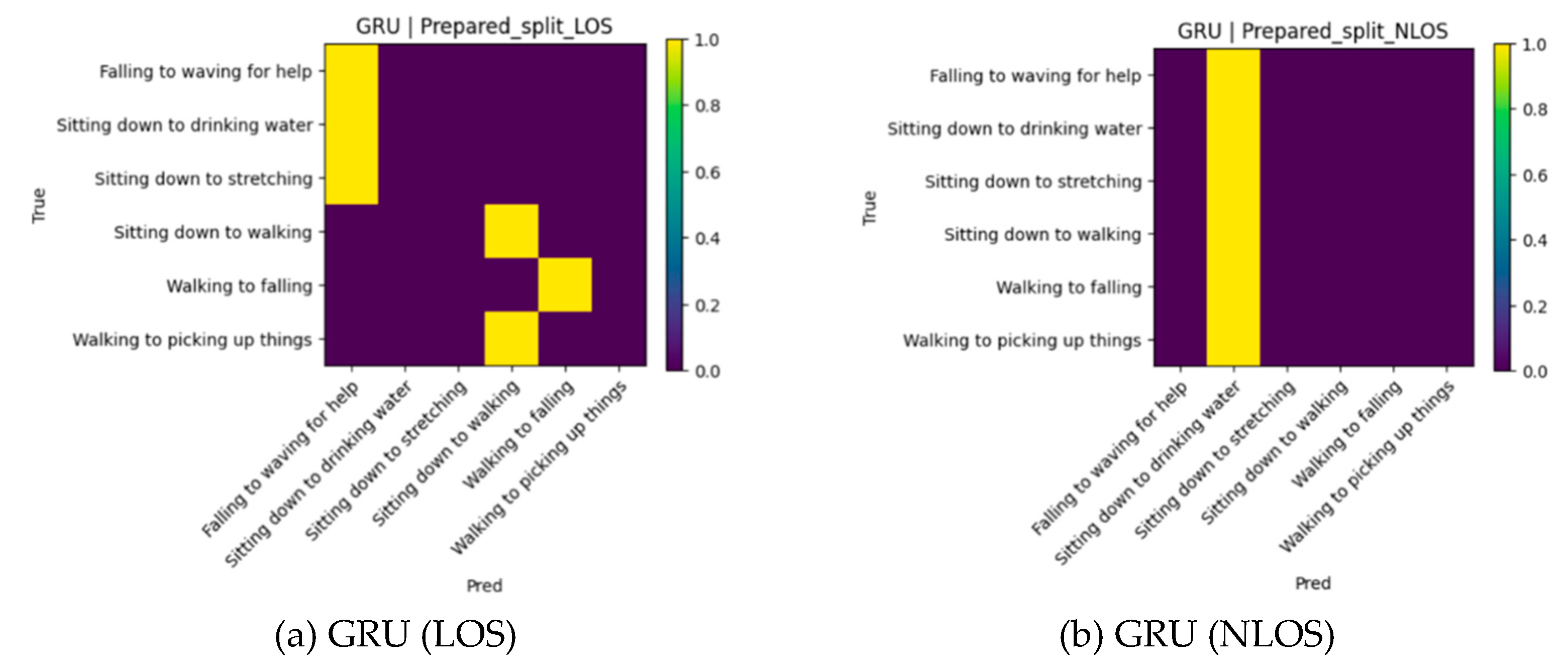
Notably, both LSTM and GRU models did not achieve satisfactory convergence in the same experimental setup, yielding only up to 33% accuracy under LOS conditions and degrading to 16.67% in NLOS conditions. This performance degradation is not attributable to training instability but instead reflects a structural mismatch between the model architectures and the input representation. Specifically, the radar range–Doppler maps employed in this study are spatial 2D tensors without an explicit temporal sequence. While recurrent architectures are designed to model sequential dependencies, CNNs are inherently better suited for capturing localized spatial correlations. Consequently, the inferior performance of RNN-based models further supports the adoption of CNN backbones for mmWave radar–based HAR.
6.4. Summary of Observations
The above results show that the CNN baseline is highly sensitive to the training order under NLOS conditions. Under the default Light to Medium to Hard order, the model exhibits unstable cross-phase performance, indicating pronounced order sensitivity. Although altering the training sequence can alleviate forgetting, the overall behavior remains inconsistent across phases. This suggests that sequential adaptation in CNNs is strongly influenced by domain order, limiting stable knowledge retention across domains.
When the training order is changed to Light to Hard to Medium, forgetting is largely alleviated and backward transfer becomes positive. However, the accuracy across different phases remains unstable, indicating that the CNN baseline lacks stable cross-phase generalization and strongly depends on the training order.
This behavior arises because the CNN baseline has no explicit mechanism to protect previously learned knowledge. During sequential training, convolutional layers are continuously updated to adapt to the current domain, which can disrupt representations learned from earlier phases. This issue is exacerbated in non-stationary NLOS environments, where signal characteristics vary substantially across phases.
In contrast, the proposed FCL framework demonstrates improved stability and robustness. Its cross-phase performance remains consistent across different domains, primarily due to two design choices. First, selective freezing preserves low-level radar features during adaptation. Second, L2-SP regularization constrains parameter drift between consecutive phases. As a result, FCL effectively mitigates forgetting and achieves positive backward transfer, indicating that learning new domains can also benefit earlier ones. These results demonstrate that FCL supports stable continual learning and promotes the learning of domain-invariant radar features under changing NLOS conditions.
7. Conclusion
Overall, the results demonstrate that conventional CNN-based sequential learning is ill-suited to non-stationary radar environments. By integrating federated learning with selective freezing and regularization, the proposed FCL framework provides a practical solution for stable and privacy-preserving mmWave-based human activity recognition. FCL achieves consistently high accuracy (approximately 97–98%) under both LOS and NLOS conditions, exhibits low forgetting with positive backward transfer, and remains largely insensitive to training order. In addition, the federated design enables collaborative learning across distributed radar devices without sharing raw data. Together, these results indicate that FCL can effectively adapt to new environments while preserving prior knowledge, making it well suited for real-world mmWave-based HAR applications. Although the proposed FCL framework demonstrates strong robustness and stability across different domains, there is still room for improvement.
Future studies could further focus on validating the model in real-world environments with multiple or moving radar devices to confirm its generalization beyond simulated NLOS data. Using lightweight backbones such as MobileNetV3 or ConvNeXt-Tiny can make the system faster and more efficient for real-time and on-device inference. It is also useful to combine mmWave radar with other sensors to get richer features and reduce confusion in activity recognition. Future work can also study adaptive client sampling, knowledge sharing between clients, and continual learning strategies to make large federated HAR systems more scalable and efficient. These improvements can make federated continual learning more practical and flexible in real-world environments.
Author Contributions
Conceptualization, Y.A. and B.-C.S.; methodology, Y.A and B.-C.S.; software, Y.A. and B.-C.S.; validation, Y.A.; formal analysis, Y.A.; investigation, Y.A.; data curation, Y.A.; writing—original draft preparation, Y.A.; writing—review and editing, Y.A. and B.-C.S.; supervision, B.-C.S. All authors have read and agreed to the published version of the manuscript.
Funding
This research received no external funding.
Institutional Review Board Statement
Not applicable.
Informed Consent Statement
Not applicable.
Data Availability Statement
The data presented in this study are available from the corresponding author upon reasonable request.
Acknowledgments
The authors would like to thank Tharuka Govinda Waduge for his valuable guidance and constructive suggestions regarding the structure, clarity, and presentation of the journal manuscript. The author has reviewed and edited the output and takes full responsibility for the content of this publication.
Conflicts of Interest
The authors declare no conflicts of interest.
References
- Soumya, A.; Krishna Mohan, C.; Cenkeramaddi, L.R. Recent Advances in mmWave-Radar-Based Sensing, Its Applications, and Machine Learning Techniques: A Review. Sensors 2023, 23, 8901. [Google Scholar] [CrossRef] [PubMed]
- Yu, Q.; Han, C.; Bai, L.; Choi, J.; Shen, X. Low-Complexity Multiuser Detection in Millimeter-Wave Systems Based on Opportunistic Hybrid Beamforming. IEEE Trans. Veh. Technol. 2018, 67, 10129–10133. [Google Scholar] [CrossRef]
- Min, X.; Ye, Y.; Xiong, S.; Chen, X. Computer Vision Meets Generative Models in Agriculture: Technological Advances, Challenges and Opportunities. Applied Sciences 2025, 15, 7663. [Google Scholar] [CrossRef]
- Yang, Y.; Chen, C.; Jia, Y.; Cui, G.; Guo, S. Non-Line-of-Sight Target Detection Based on Dual-View Observation with Single-Channel UWB Radar. Remote Sensing 2022, 14, 4532. [Google Scholar] [CrossRef]
- Degu Workneh, A.; Gmira, M. Scheduling Algorithms: Challenges Towards Smart Manufacturing. Int. j. electr. comput. eng. syst. (Online) 2022, 13, 587–600. [Google Scholar] [CrossRef]
- Jiang, W.; Wu, K.; Gan, H.S. Knee Osteoarthritis Diagnosis Integrating Meta-Learning and Multi-Task Convolutional Neural Network. Proc. IEEE International Conference on Bioinformatics and Biomedicine (BIBM), Lisbon, Portugal, December 2024. [Google Scholar]
- Jordan, T.S. Using Convolutional Neural Networks for Human Activity Classification on Micro-Doppler Radar Spectrograms. Proc. SPIE Sensors, and Command, Control, Communications, and Intelligence (C3I) Technologies for Homeland Security, Defense, and Law Enforcement Applications XV, Baltimore, MD, U.S.A, May 2016. [Google Scholar]
- El Hail, R.; Mehrjouseresht, P.; Schreurs, D.M.M.-P.; Karsmakers, P. Radar-Based Human Activity Recognition: A Study on Cross-Environment Robustness. Electronics 2025, 14, 875. [Google Scholar] [CrossRef]
- Sheeny, M.; Wallace, A.; Wang, S. RADIO: Parameterized Generative Radar Data Augmentation for Small Datasets. Applied Sciences 2020, 10, 3861. [Google Scholar] [CrossRef]
- Zheng, P.; Zhang, A.; Chen, J.; Qi, F. Radar-Based Cross-Domain Human Behavior Recognition Using Physics-Informed Data Augmentation and Multi-Source Domain Adversarial Neural Network. IEEE J. Biomed. Health Inform. 2025, 1–14. [Google Scholar] [CrossRef] [PubMed]
- Wang, Z.; Kang, K. Adaptive Temporal Attention Mechanism and Hybrid Deep CNN Model for Wearable Sensor-Based Human Activity Recognition. Sci Rep 2025, 15, 33389. [Google Scholar] [CrossRef] [PubMed]
- Harmanny, R.I.A.; De Wit, J.J.M.; Cabic, G.P. Radar Micro-Doppler Feature Extraction Using the Spectrogram and the Cepstrogram. Proc. 11th European Radar Conference (EuRAD), Rome, Italy, October 2014. [Google Scholar]
- Wen, J.; Zhang, Z.; Lan, Y.; Cui, Z.; Cai, J.; Zhang, W. A Survey on Federated Learning: Challenges and Applications. Int. J. Mach. Learn. & Cyber. 2023, 14, 513–535. [Google Scholar] [CrossRef]
- Kairouz, P.; McMahan, H.B.; Avent, B.; Bellet, A.; Bennis, M.; et al. Advances and Open Problems in Federated Learning. FNT in Machine Learning 2021, 14, 1–210. [Google Scholar] [CrossRef]
- Li, X.; Grandvalet, Y.; Davoine, F. Explicit Inductive Bias for Transfer Learning with Convolutional Networks. Proc. Machine Learning Research; Stockholm Sweden, July 2018. [Google Scholar]
- McMahan, H.B.; Moore, E.; Ramage, D.; Hampson, S. Communication-Efficient Learning of Deep Networks from Decentralized Data. Proc. 20th International Conference on Artificial Intelligence and Statistics, Fort Lauderdale, FL, U.S.A., April 2017. [Google Scholar]
- Lopez-Paz, D.; Ranzato, M. Gradient Episodic Memory for Continual Learning. Proc. 31st International Conference on Neural Information Processing Systems (NIPS), Long Beach, CA, U.S.A, December 2017. [Google Scholar]
- Plested, J.; Gedeon, T. Deep Transfer Learning for Image Classification: A Survey. arXiv arXiv:2205.09904. [CrossRef]
- Wu, X.; Ling, Z.; Zhang, X.; Ma, Z.; Deng, W. Human Similar Activity Recognition Using Millimeter-Wave Radar based on CNN-BiLSTM and Class Activation Mapping. Eng 2025, 6, 44. [Google Scholar] [CrossRef]
- Liu, J.; He, P.; Alhusaini, N.; Li, W.; Zhao, L.; Li, S. RADHOME: Radar based Human Activity Dataset in Home Environments. Mendeley Data 2025, V1. [Google Scholar] [CrossRef]
Figure 2.
Heat map visualization of cross-phase validation accuracy matrix of FCL on NLOS dataset.
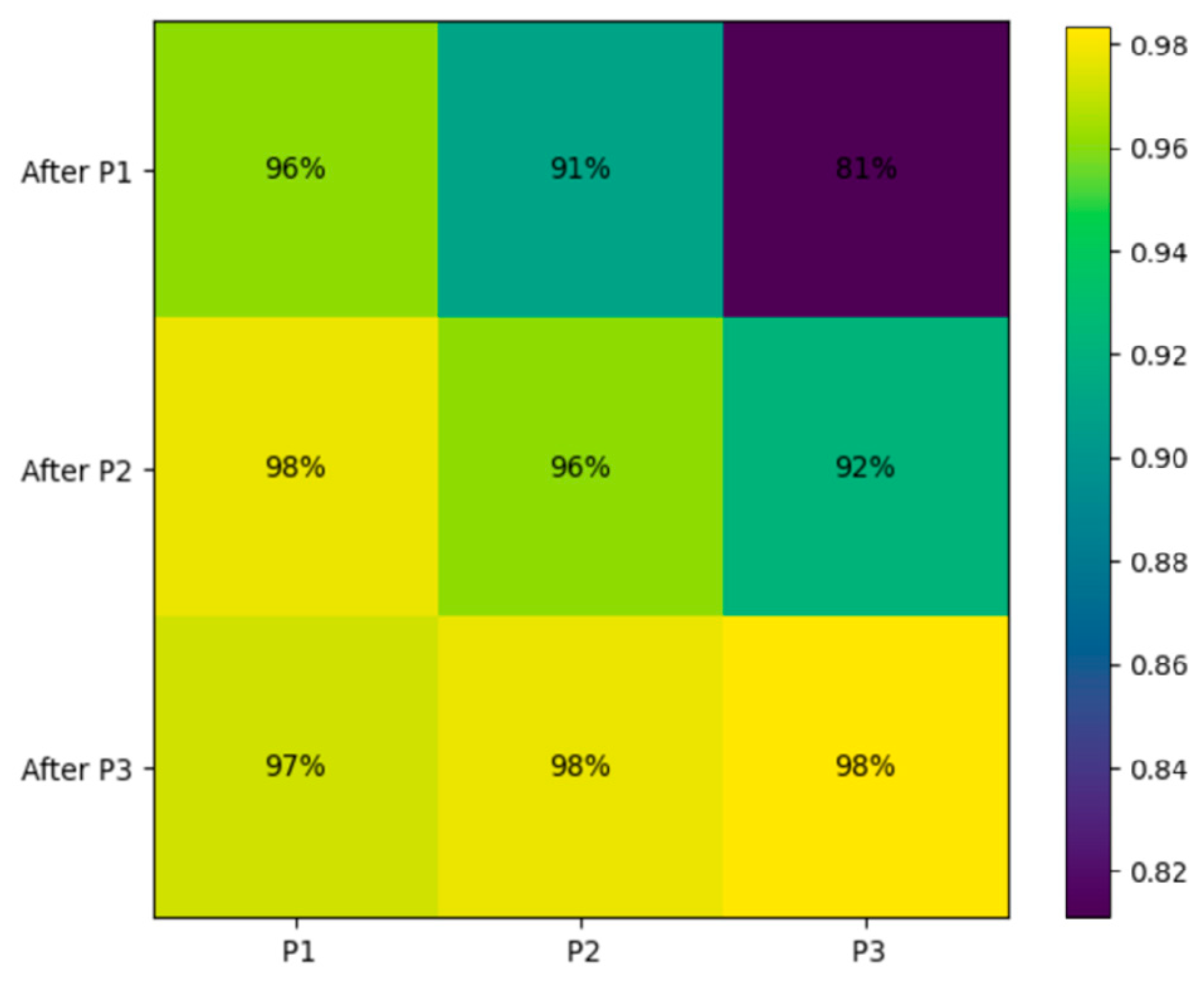
Figure 3.
Heatmap visualization of cross-phase validation accuracy for CNN baseline under: (a) default order (Light, Medium, Hard); (b) swapped order (Light, Hard, Medium).
Figure 3.
Heatmap visualization of cross-phase validation accuracy for CNN baseline under: (a) default order (Light, Medium, Hard); (b) swapped order (Light, Hard, Medium).
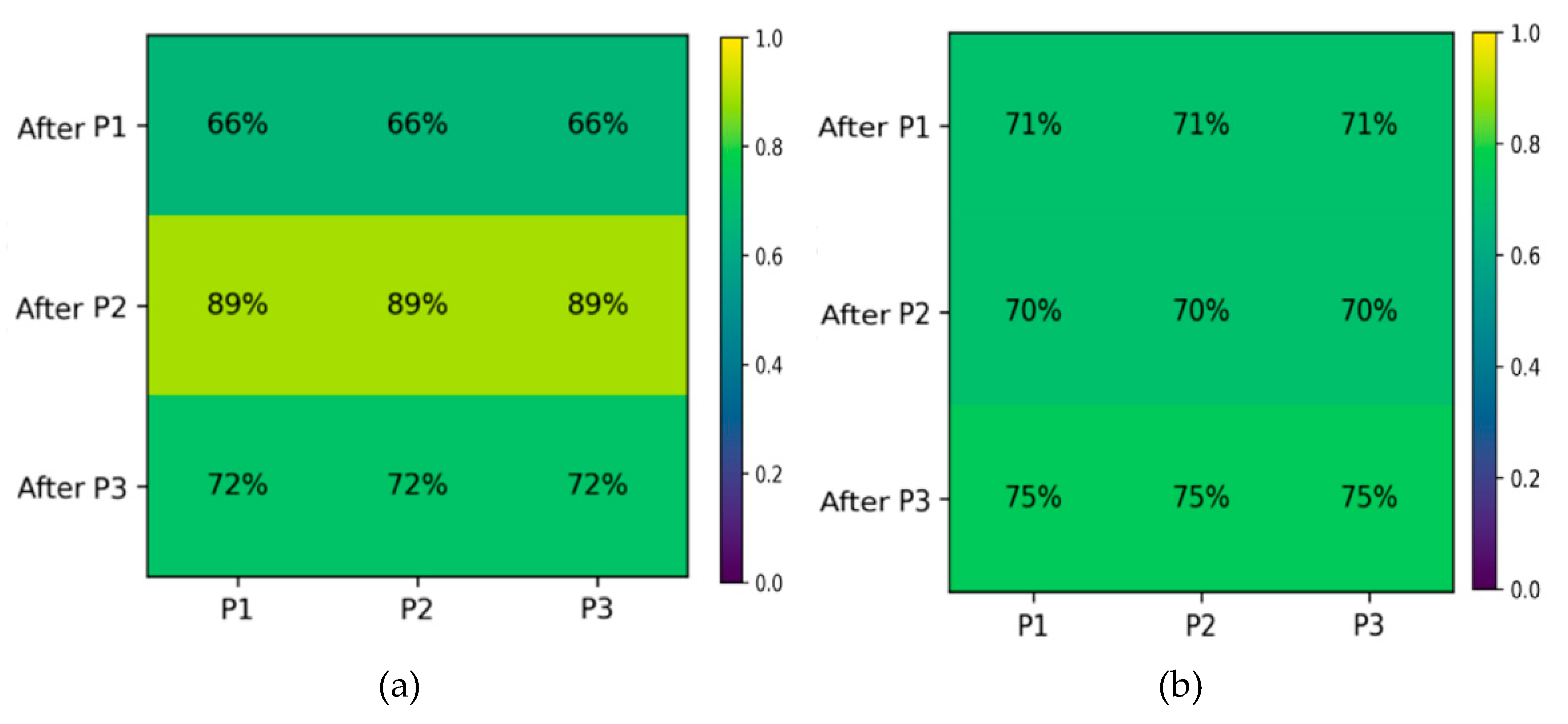
Figure 4.
Comparison of cross-phase validation accuracy between CNN and FCL.
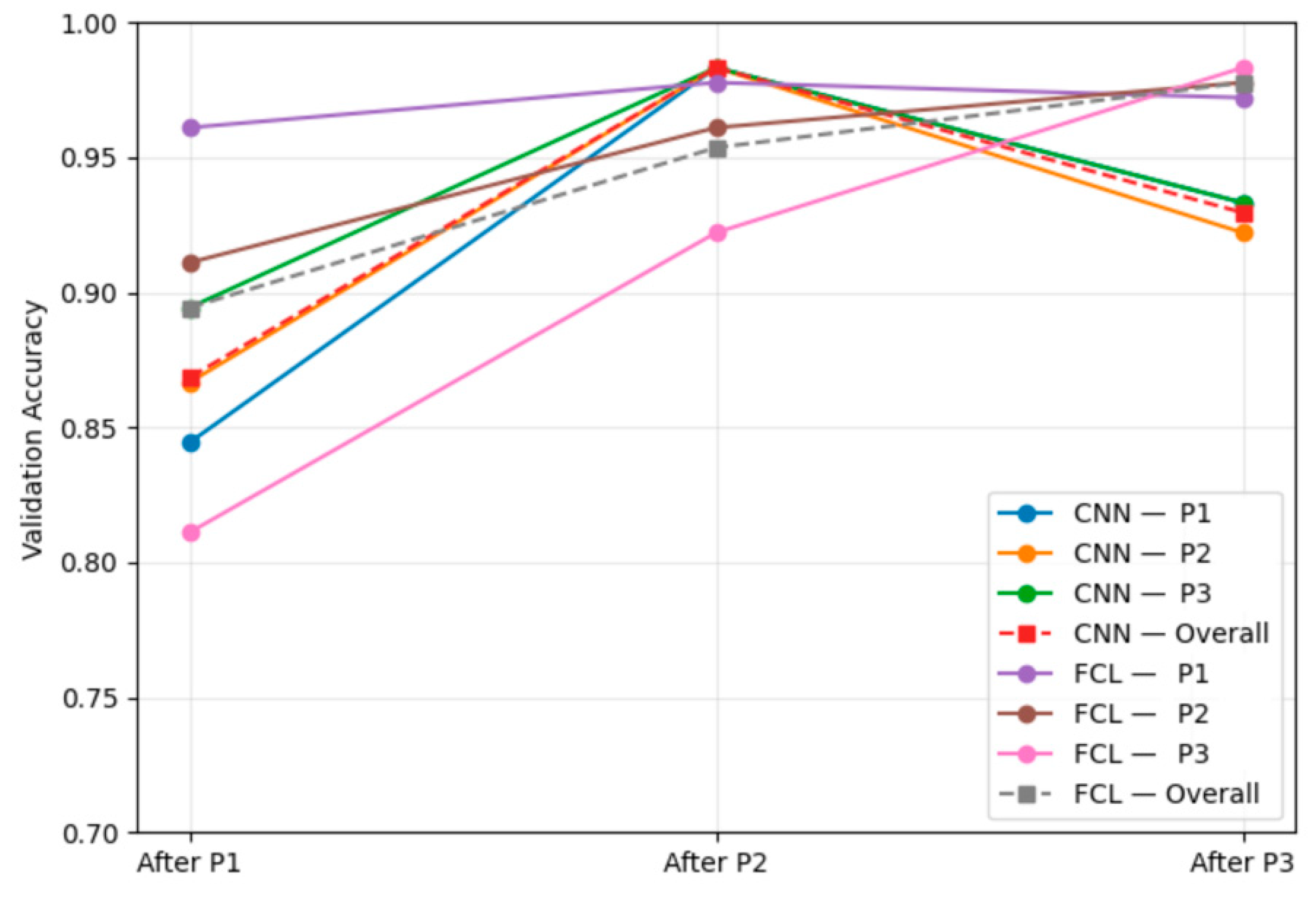
Table 4.
Cross-phase validation accuracy for the CNN-only sequential baseline.
| Server Snapshot | P1 | P2 | P3 |
|---|---|---|---|
| After P1 | 0.9611 | 0.9667 | 0.9944 |
| After P2 | 0.9611 | 0.9833 | 0.9944 |
| After P3 | 0.9833 | 0.9611 | 0.9834 |
Table 5.
Cross-phase validation accuracy results of FCL on NLOS dataset.
| Server Snapshot | P1 | P2 | P3 |
|---|---|---|---|
| After P1 | 96% | 91% | 81% |
| After P2 | 98% | 96% | 92% |
| After P3 | 97% | 98% | 98% |
Table 6.
Overall continual-learning metrics of FCL on NLOS.
| Metric | Value |
|---|---|
| Final Test Accuracy | 97.78% |
| Final Test Macro-F1 | 97.79% |
| Average Forgetting (AF) | 0.19% |
| Backward Transfer (BWT) | +1.39% |
Table 8.
Cross-phase validation performance of CNN baseline under different sequential orders.
| Configuration | ACC (%) | AF (%) | BWT (%) | Stability |
|---|---|---|---|---|
| CNN (default order) | 65.56–89.44–72.22 | 1.11 | 0.00 | Unstable, order-sensitive |
| CNN (swapped order) | 70.56–70.00–75.00 | 0.00 | +4.72 | Slightly improved, but order-sensitive |
Table 9.
CNN vs. RNN (LSTM/GRU) on LOS and NLOS datasets.
| Model | Train Domain | Test Domain | Accuracy (%) | F1(%) |
|---|---|---|---|---|
| RNN (LSTM) | LOS | LOS | 33.33 | 25.00 |
| NLOS | NLOS | 16.67 | 4.76 | |
| LOS | NLOS | 50.00 | - | |
| NLOS | LOS(cross) | 16.67 | - | |
| RNN (GRU) | LOS | LOS | 50.00 | 36.11 |
| NLOS | NLOS | 16.67 | 4.76 | |
| LOS | NLOS(cross) | 33.33 | - | |
| NLOS | LOS(cross) | 16.67 | - | |
| CNN (static) | LOS | LOS | 100.00 | 100.00 |
| CNN (static) | NLOS | NLOS | 94.44 | 94.520 |
Disclaimer/Publisher’s Note: The statements, opinions and data contained in all publications are solely those of the individual author(s) and contributor(s) and not of MDPI and/or the editor(s). MDPI and/or the editor(s) disclaim responsibility for any injury to people or property resulting from any ideas, methods, instructions or products referred to in the content. |
© 2025 by the authors. Licensee MDPI, Basel, Switzerland. This article is an open access article distributed under the terms and conditions of the Creative Commons Attribution (CC BY) license (http://creativecommons.org/licenses/by/4.0/).
Copyright: This open access article is published under a Creative Commons CC BY 4.0 license, which permit the free download, distribution, and reuse, provided that the author and preprint are cited in any reuse.


