Submitted:
19 December 2025
Posted:
22 December 2025
You are already at the latest version
Abstract
In this paper, we investigate the lexicographic and colexicographic orderings of m-ary vectors of length n, as well as the mirror (left-recursive) reflected Gray code, complementing the classical m-ary reflected Gray code. We present efficient algorithms for generating vectors in each of these orders, each achieving constant amortized time per vector. Additionally, we propose algorithms implementing the four fundamental functions in generating combinatorial objects—successor, predecessor, rank, and unrank—each with time complexity Θ(n). The properties and the relationships between these orderings and the set of integers {0,1,…,mn−1} are examined in detail. We define explicit transformations between the different orders and illustrate them as a digraph very close to the complete symmetric digraph. In this way, we provide a unified framework for understanding ranking, unranking, and order conversion. Our approach, based on emulating the execution of nested loops, proves to be powerful and flexible, leading to elegant and efficient algorithms that can be extended to other combinatorial generation problems. The mirror m-ary Gray code introduced here has potential applications in coding theory and related areas. By providing an alternative perspective on m-ary Gray codes, we aim to inspire further research and applications in combinatorial generation and coding.
Keywords:
combinatorial generation
; m-ary vectors generation
; lexicographic order
; colexicographic order
; m-ary reflected Gray code
; mirror m-ary reflectedGray code
; ranking
; unranking
; successor
; predecessor
1. Introduction
The generation of combinatorial objects in various orderings is a fundamental and widely studied topic in the literature on combinatorial algorithms [1,2,3,4,5,6] and many others. The most well-known types of orderings of generated objects are the lexicographic order and the minimum-change order, known as Gray code order, each having numerous varieties [1,2,3,6,7,8,9], etc. Due to their wide range of application, which are difficult to enumerate exhaustively, these orderings are of great importance for both theory and practice.
The lexicographic order of all m-ary vectors of length n is a classical concept. Considering these vectors as n-digit numbers in a number system with radix m, their lexicographic order corresponds to the increasing numerical order of the numbers when read from left to right. The colexicographic order of these numbers (resp. vectors) is obtained by sorting them based on their digits (resp. coordinates) from right to left, i.e., from the least significant to the most significant digit [6,9]. In [3], Section 7.1.3. (Bit reversal, p. 144), Knuth uses the term left-right mirror image in the context: For our next trick, let’s change to its left-right mirror image, … As we will see, each vector in the colexicographic order is the left-right mirror image of the corresponding vector in the lexicographic order, and vice versa. Based on this relationship and additional arguments, we propose that the classical m-ary reflected Gray code be divided into two different types. For , these are the binary reflected Gray code and the mirror (left-recursive) binary Gray code [10], while for , the standard type is presented in [11]. In this work, we introduce and examine the second type, referred to as the mirror (left-recursive) m-ary reflected Gray code. We propose algorithms for generating m-ary vectors of length n in lexicographic and colexicographic orders, as well as in the mirror m-ary reflected Gray code, and discuss their recursive implementations, highlighting both advantages and limitations. Furthermore, we present a general approach for generating these vectors by emulating the execution of n nested loops, which improves the clarity and adaptability of the algorithms. Corresponding C code is provided for straightforward use.
The functions for computing the predecessor and successor, as well as for ranking and unranking, play an important role in the generation of combinatorial objects [1,3,4,6]. Most of the authors always consider these functions (if they are created) when generating given combinatorial objects. For all orderings considered here, we propose the four basic functions, illustrated in Figure 1, with different algorithms for different orderings.
The proposed algorithms are designed for , considering that for more efficient implementations using bitwise representations and operations are possible.
This article is organized as follows. Section 2 presents the generation of all m-ary vectors in lexicographic order, including the basic concepts, their properties, and the corresponding algorithms. Section 3 deals with the colexicographic order of the same vectors and has a similar structure, adding Remark 1 and Theorem 3, which describe the relationship between lexicographic and colexicographic order. Section 4 poses the problem of the two versions of the m-ary Gray reflection code that are used in the literature but are not distinguished. We present several arguments supporting the need to differentiate these versions and assign them distinct names. We then describe the generation of m-ary vectors in the Gray reflection code, together with the successor and predecessor functions, after deriving the main concepts and comparing them with the standard m-ary Gray code. Section 5 summarizes the previous sections by presenting the relationships between the considered orders and the set , the transformations between each pair of them, and the corresponding ranking and unranking functions. All of these are illustrated in Figure 3 as a digraph very close to the complete symmetric digraph , i.e., missing exactly two arcs. Section 6 contains several concluding remarks. Most of the results obtained here are original, while the rest are similar to known results.
2. Lexicographic Order of the -ary Vectors
From now on, we talk about given positive integers n and . We consider the set of integers and its n-th Cartesian power , which is the set of all m-ary vectors of length n. There are such vectors, i.e., .
2.1. Definitions, Properties and Preliminary Notes
For convenience, we define recursively as follows.
Definition 1.
The set of all m-ary vectors of length n is defined by:
where denotes the set of all vectors of prepended by k, for .
If necessary, Definition 1 can start with , which is the set of the empty vector (with 0 coordinates) corresponding to the empty word/string. When a matrix representation is needed, the vectors can be arranged as rows of a matrix of size .
Let and be arbitrary vectors of . The non-negative integer is called the serial number of , i.e., the conversion of the n-digit radix-m number into decimal. Usually, the serial number differs from the rank, which is the position of in the sequence of vectors according to a chosen ordering, and is also called the sequential, ordinal number of . The serial number is unique (like the serial number of a device), while the rank of the vector changes depending on the selected order of the vectors.
The vector precedes lexicographically the vector and is denoted by if or there exists an integer k, , such that and for all . The relation on is defined as follows: for arbitrary vectors and , whenever . It is obvious that is reflexive, strictly antisymmetric (i.e., for any , , either or and then and are lexicographically comparable) and transitive. Therefore, is a relation of total order on and all vectors of can be uniquely ordered according to in lexicographical order.
Theorem 1.
Let the vectors of be defined as in Definition 1. Then:
a) they are in lexicographic order;
b) their serial numbers form the sequence ;
c) for each vector α in the lexicographic order of .
The theorem can be proven by induction on n following Definition 1 (see the proof of Theorem 2). Its statement is illustrated in Table 1 for .
2.2. Generation of the Vectors of in Lexicographic Order
There are at least two ways to generate all vectors of in lexicographic order. Following Theorem 1, the first involves converting each integer from 0 to into a radix-m number and, if necessary, prepending leading zeros to obtain an n-digit representation. This operation (function) is known as unranking, and its inverse operation (function) is referred to as ranking. Both operations are based on the Horner rule:
In the algorithms below, the vectors are stored in global one-dimensional arrays: a for the lexicographic order, c for the colexicographic order, and g for the Gray code. They are defined appropriately so that their zeroth or last element can be used as a sentinel or left unused for better efficiency. Thus, the coordinates of the vectors occupy the elements with indices .
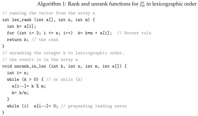
Obviously, each of these functions has a time complexity , although the operations integer division and computing the reminder modulo m are time-consuming operations when m is not a power of 2.
The second way to generate the vectors of in lexicographic order is by using of n nested loops. This is a special case of the general problem of generating all n-tuples in a mixed radix system1, which is considered by Knuth [3] [Sect. 7.2.1.1. Mixed-radix generation, Algorithm M] and Arndt [1] [Chapter 9. Mixed radix numbers]. The values of the loop variables in the body of the innermost loop form the current vector of length n—the idea is shown in the next code fragment.
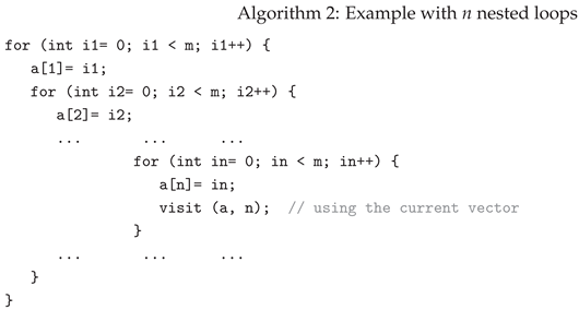
Writing code with n nested loops is hard-coding and bad practice. So we will emulate the execution of n nested loops, where each has an initial value of 0, a final value of , and a step of 1. The emulation algorithm uses the array a, whose elements contain the values of the loops variables (see the code above) and are the coordinates of the current vector represented by a. As in the generation of other combinatorial objects in [1,2,3,12,13], it is convenient to formulate and use a rule of succession for the vectors of in lexicographic order: To obtain the next vector after the current one in the array a:
1) Scan the elements of the array a from right to left (i.e., a[n], a[n-1], etc.), looking for the first element that has not reached its final value . During the scan, set each scanned element to 0.
2) If such an element is found, increase its value by 1. Otherwise, terminate, as the last vector was in the array a.
We examine the emulation algorithm in detail, as it is the basis for the development of the other algorithms presented here. They all use the printn function instead of the more general visit function used in [1,2,3]. It prints the current vector with its ordinal number (rank) in the generated sequence, using the global variable ord_num. Here is their C code.
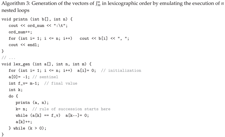
The correctness of this algorithm can be easily proven by induction on n. Regarding its time complexity: obviously, the algorithm performs operations to generate each vector after the current one and therefore a total of operations. Let us estimate its time complexity more precisely. To generate all vectors, the while loop of the algorithm checks times the last element a[n], times the penultimate element a[n-1] and so on, times the first element a[1]. In total, the while loop performs comparisons and the same number of assignments and subtractions. In the body of the main loop do ... while, other comparisons, assignments, and additions are performed (except for the operations in the function printn). Therefore, the total time complexity of the algorithm is to generate all vectors. Thus, the average time to generate one vector is constant and the algorithm is of the type Constant Amortized Time (CAT) algorithm [6]. The space complexity is and therefore it and the time complexity are of the same type as of a loopless algorithm.
Here is the code for the corresponding recursive algorithm.

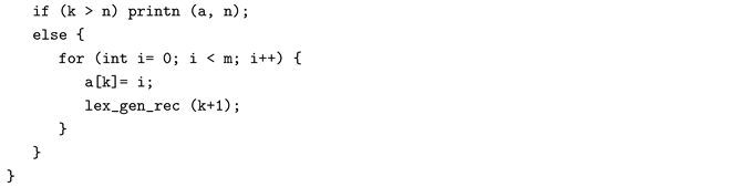
This function must be invoked using lex_gen_rec(1). So it starts by executing the first (outermost) loop—see Algorithm 2—and each subsequent function call continues with the execution of the next (second, third, etc.) loop, with the n-th call executing the n-th (innermost) loop, and with the -st call reaching the bottom of the recursion. This fully corresponds to Definition 1 and therefore, Algorithm 4 is correct.
As we said, the function lex_gen_rec makes additional calls to reach the bottom of the recursion. Table 2 is part of a larger table and shows the trend of the percentage ratio between the number of recursive calls and the number of vectors generated, depending on the values of n and m. Despite the additional execution time of the recursive calls (each of them for constant time), despite the additional calls, Algorithm 4 is also a CAT algorithm. It is slower, but shorter and probably clearer than the non-recursive Algorithm 3.
2.3. Successor and Predecessor Functions in the Lexicographic Order
Using the the rule of succession and the code of Algorithm 3, writing the functions for computing the successor and predecessor of the current vector becomes straightforward. Both of the following functions modify the vector stored in the array a to compute the corresponding next or previous vector in the same array. The function lex_successor implements the rule of succession. The function lex_predecessor works in the opposite direction: it scans the elements of a from right to left, looking for an element with a positive value (since 0 is the minimum). During this scan, scanned elements are reset from 0 to . When such an element is found, its value is decremented by 1. Finally, note that the last vector has no successor, and the first vector has no predecessor. Similar functions for mixed radix numbers are described in [1] [Sect. 9.1].
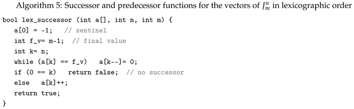
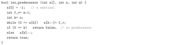
It is obvious that each of the two functions has running time .
3. Colexicographic Order of the Vectors of
Of the various orders associated with the lexicographic order, the colexicographic (or colex) order is the most prominent and useful alternative to the lexicographic ordering [4]. It is used in generating combinations, permutations, partitions, bitstrings, related structures such as necklaces and Lyndon words, etc. [1,3,4,6,14] and others. Arndt notes: The co-lexicographic (or simply colex) order is obtained by sorting with respect to the reversed strings and The sequence for co-lexicographic (or colex) order is such that the sets, when written reversed, are ordered lexicographically [1] [p. 172, p. 177]. Ruskey [6] [p. 59] introduces the Colex Superiority Principle: Try to use colex order (right-to-left array filling) whenever possible. It will make your programs shorter, faster, and more elegant and natural. That is why we are consider it here. To the best of our knowledge, there is no prior publication that treats the complete generation of all m-ary vectors of length n in colexicographic order, including explicit algorithms for ranking/unranking functions. The present work appears to be the first to consider this case systematically.
3.1. Definitions, Properties and Preliminary Notes
Definition 2.
The set of all m-ary vectors of length n is defined by:
where denotes the set of all vectors of suffixed by k, for .
Analogously to the lexicographic order, the vector precedes colexicographically the vector and is denoted by , if or there exists an integer k, , such that and for all . The corresponding relation is defined on analogously: for arbitrary vectors and , whenever . Then is also reflexive, strictly antisymmetric and transitive and so it is a relation of total order on , i.e., all vectors of can be uniquely ordered according to in colexicographic order.
Theorem 2.
Let the vectors of be defined as in Definition 2. Then:
a) they are in colexicographic order;
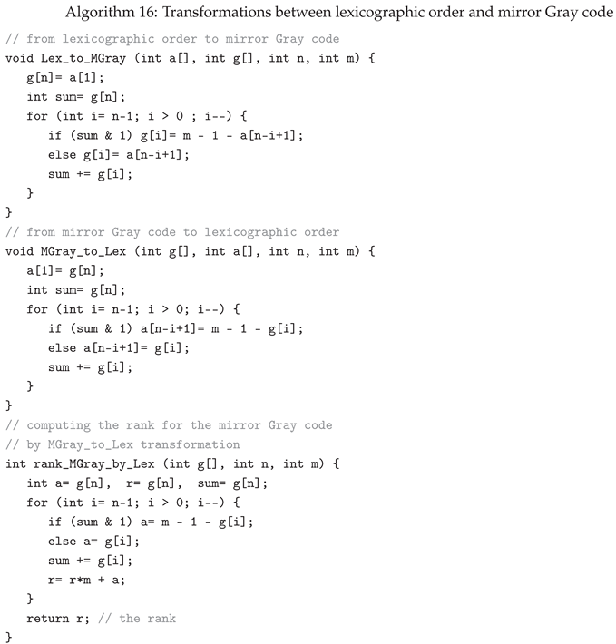
b) the sequence of their serial numbers, denoted by , is:
where means that the serial numbers of all vectors from are multiplied by m, then k is added to each of them, for .
Proof.
We will prove the theorem by mathematical induction on n, following Definition 2.
1) For , both statements are obviously true.
2) Let us assume that for and for the vectors of :
a) they are in colexicographic order;
b) is the sequence of their serial numbers.
3) For the vectors of it follows that:
a) They are in colexicographic order, due to the inductive hypothesis (the vectors of are in colexicographic order) and each vector of the type precedes colexicographically each vector of the type when .
b) They are obtained by taking the vectors of exactly m times and appending a new coordinate to each copy. In other words, , . This means that the vectors of are obtained by shifting the vectors of by one position to the left, and the new coordinate k occupies the n-th position in each of them, for . According to the definition of the serial number, this shift corresponds to multiplication by m. Thus, and in accordance with the inductive proposition, the serial numbers are obtained from the corresponding serial numbers multiplied by m and then adding k to each of them, for . Hence:
Thus, the theorem holds. □
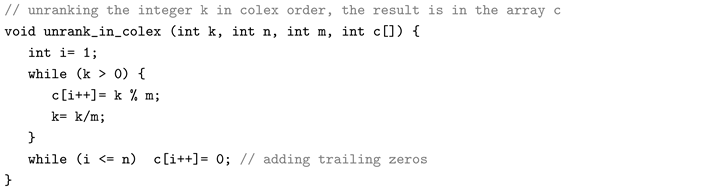
We have developed an algorithm that generates the sequence of the serial numbers of the vectors of . Its time complexity is , i.e., it is a CAT algorithm. However, its space complexity is of the same type. To obtain the vectors of in colexicographic order, it is only necessary to transform each of its terms into an m-ary vector with n coordinates. For example, the function unrank_in_colex (see Algorithm 6) can be used for this purpose, in time per term. But the overall time and space complexity of this approach is not acceptable.
Generating the vectors in lexicographic order and then applying the coordinate-reversal function (see Remark 1) gives the same time complexity but only space complexity.
Remark 1.
Before considering the algorithms for the colexicographic order, it is important to note:
- 1.
- Relationship between the lexicographic and colexicographic order: The colexicographic order can be obtained from the lexicographic order and vice versa, by reflecting the coordinate order of the vectors in the respective ordering. That is, , iff [6].
- 2.
- We define the coordinate-reversal function φ such that , and for any vector , . Thus, the coordinates of are left-right mirror image of those of α and vice versa [3] [p. 144]. Obviously φ is a bijection and also and therefore φ is an involution.
- 3.
- The fixed points of the function φ are the palindromes, i.e., . Their number is .
- 4.
- Comparing Definition 1 and Definition 2 and in accordance with Theory of Formal Languages, we note that Definition 1 uses right recursion (or substitution—the words are derived from left to the right and therefore the rightmost symbols change the fastest, compared to the leftmost symbols, which change the slowest), while Definition 2 uses left recursion.
From the statements in Remark 1 it follows immediately:
Theorem 3.
If the vectors of are listed in lexicographic order and we apply the coordinate-reversal function φ to each vector, then the resulting sequence is the colexicographic order of these vectors, and conversely. Moreover:
- 1.
- For every vector α in lexicographic order, , where is the corresponding vector in colexicographic order. Also, if and only if , that is, α is a palindrome.
- 2.
- Let L and C be matrices representing the vectors of , listed in lexicographic and colexicographic order, respectively. Then the i-th column of L coincides with the -st column of C, for .
3.2. Generation of the Vectors of in Colexicographic Order
We now present the algorithms for colexicographic order. They follow Definition 2, Theorem 2 and Remark 1 and are analogous to the corresponding algorithms for lexicographic order. Hence their correctness can be proven in the same way. Their time complexity is of the same type as that of the corresponding algorithms for lexicographic order. So, instead of analogous reasoning, we provide only brief comments.
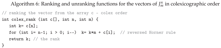
We start with the functions for ranking a vector and unranking an integer k, , into a vector of in colexicographic order. They use the following reverse version of the Horner rule:
Another way to generate is to simply change the assignments in Algorithm 2: a[n]= i1; a[n-1]= i2; ..., a[1]= in. This makes the following algorithms more understandable.
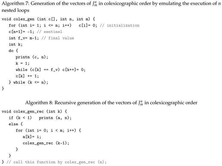
Everything mentioned in the comparison of recursive and non-recursive algorithms for generating in lexicographic order (including Table 2) applies equally to the corresponding algorithms for colexicographic order.
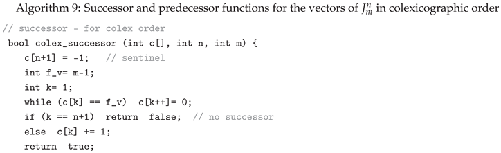
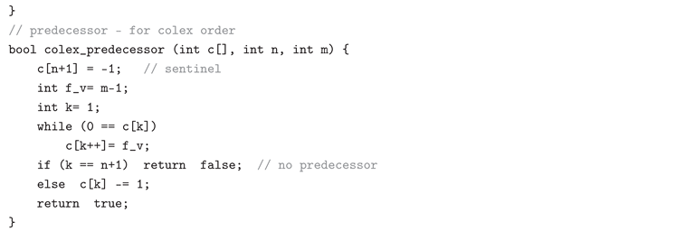
3.3. Successor and Predecessor Functions in the Colexicographic Order
4. Mirror -Ary Reflected Gray Code
We recommend that the reader refer to the open access article [11], as we cannot repeat its content regarding m-ary reflected Gray code here.
4.1. About the Two Versions of the m-ary Reflected Gray Code
This section is a natural extension of [11] and a generalization of [10]. In the first article, we examined in detail the m-ary reflected Gray code, as well as the m-ary modular (or shifted) Gray code. In the second article, we introduced and investigated a version of the Binary Reflected Gray Code (BRGC), called the mirror (left-recursive) binary Gray code, and compared it with the standard BRGC. We also argued for treating these two codes as distinct. Most of these arguments remain valid for the m-ary reflected Gray code, and additional sources and reasons support this distinction. Taken together, they convincingly show that these two versions of the m-ary reflected Gray code should be considered distinct and, consequently, should have different names. Therefore, we refer to the new version as the mirror m-ary reflected Gray code, or more precisely, the left-recursive (L-R) m-ary reflected Gray code, and to the standard version as the m-ary reflected Gray code, or more precisely, the right-recursive (R-R) m-ary reflected Gray code—see Definition 3 and the following paragraph. The terms left-recursive and right-recursive (proposed by Krassimir Manev) accurately characterize the two versions, since the order of the coordinates of any vector in one version is the mirror image of the order of the coordinates of the corresponding vector in the other version. Hence, the term mirror may refer to either of them. Below, we present the main arguments supporting this distinction.
- Relationship between the lexicographic and colexicographic order. The connection between the lexicographic and colexicographic order of the m-ary vectors is given by the coordinate-reversal function defined in Remark 1. Although these orders appear closely related, they are distinct and have separate names. The same relationship exists between the m-ary reflected Gray code and its mirror version. This justifies distinguishing them and calling them by different names.
-
Ambiguities in the literature. Many authors, when discussing an m-ary reflected Gray code, actually talk about a mirror m-ary reflected Gray code, or talk about both codes using the same name. When readers are not careful or do not distinguish between these codes, they can confuse them. For example:
- (a)
-
In [5] the authors first give a right-recursive definition of BRGC and show an example of it. They also define the transition sequence, where the coordinates are numbered from right to left, and emphasize the connection between it and the generation of the codewords. They also give a left-recursive definition of BRGC, but treat the two codes as the same code. In [12,13], the authors define and use only the left-recursive (mirror) BRGC and show the generated codewords. They formulate and prove the rule of succession for this code—which coordinate must be changed in the current codeword to obtain the next codeword, in fact the next term of the transition sequence. The same, but more thoroughly and in an optimized way, is done in [3] [Algorithm G].We can summarize: all these algorithms generate BRGC when the coordinates are numbered from right to left, for example . For each , the i-th coordinate of the current vector is stored in element g[i] of array g. Thus, the algorithms output BRGC if the array g is printed from right to left, otherwise they output the vectors of the mirror BRGC.
- (b)
- In [6], Ruskey defines recursively (starting from the empty string) the standard BRGC and relates it to a Hamiltonian cycle on the Boolean cube, the Towers of Hanoi problem, transition sequence and the generation of BRGC from it, as well as the ranking and unranking functions for BRGC. He then presents a left-recursive definition (via formula (5.3), p. 120), which corresponds to the mirror BRGC. Ruskey explicitly notes: Note that we are appending rather than prepending. In developing elegant natural algorithms this has the same advantage that colex order had over lex order in the previous chapter. Thus, the algorithms he proposes (indirect and direct) generate the mirror BRGC.
- (c)
- In [17], the author discusses and illustrates (in Table 1) the usual (right-recursive) k-ary reflected Gray code. He derives a non-recursive algorithm that generates its codewords and outputs them from right to left. In this way, the algorithm reverses the coordinates of the generated codewords and actually generates the left-recursive k-ary reflected Gray code. In [18], the author recursively defines the usual N-ary reflected Gray code and proposes Algorithm 1, which generates its codewords. Instead of printing them, the algorithm outputs the message “codeword available”. If we print them, we observe that they are the codewords of the left-recursive N-ary reflected Gray code. The same can be seen in [19], where the authors use the same definition and algorithm.
- Algorithmic differences. The algorithms for generating the vectors of the two versions of m-ary reflected Gray code are similar, but have subtle differences, as we will see later. The same applies to the four basic functions for these versions.
4.2. Definitions, Properties and Preliminary Notes
The Gray codes under consideration are defined as follows.
Definition 3.
The sequence of vectors of , ordered in mirror m-ary reflected Gray code, is denoted by and defined as:
If then .
If then , , where:
is the m-ary reflected Gray code of length ;
is again the m-ary reflected Gray code of length , but its vectors are reflected, i.e., taken in reverse order;
denotes if k is even, or if k is odd.
The sequence of vectors of , ordered in an m-ary reflected Gray code, is denoted by . The definition of is similar to Definition 3, with the only difference that the new coordinate is added at the beginning of the vectors, instead of at the end—for example, , which means when k is even, or when k is odd, for .
After these definitions, we note that everything said in Remark 1 is valid for the m-ary Gray code and the mirror m-ary Gray code, and we will omit an analogous remark. The following assertion corresponds to Theorem 3.
Theorem 4.
If the vectors of are listed in reflected Gray code and we apply the coordinate reversal function φ to each vector, then the resulting sequence is the mirror Gray code of these vectors and vice versa. Moreover:
- 1.
- For every vector , we have , where is the corresponding vector in . Also, if and only if , that is, α is a palindrome.
- 2.
- Let M and be matrices representing the vectors of , and , respectively. Then the i-th column of M coincides with the -st column of , for .
Theorem 1 in [18] states that the m-ary reflected Gray code is a cyclic code when its radix m is even, and is not cyclic otherwise. This statements is also true for the mirror m-ary Gray code, since the two codes are related via the coordinate-reversal function.
Theorem 1 (or Theorem 2 in [18]) is important for all algorithms working with m-ary reflected Gray code in [11] and so we give its statement.
Theorem 1.
[11] Let be a codeword of the m-ary reflected Gray code for and . When is even, then , and for , is in a subsequence of digits in ascending order; otherwise, it is in a subsequence of digits in descending order.
We propose an analogous statement for the mirror m-ary reflected Gray code, which will be important for the following algorithms. It follows directly from this theorem and the last statement of Theorem 4, applied to an arbitrary row of the matrix M and its corresponding row of the matrix .
Theorem 5.
Let be an arbitrary vector from . When is even, then the coordinate belongs to a subsequence of i-th coordinates in ascending order; otherwise, it belongs to a subsequence of i-th coordinates in descending order, for .
4.3. Generation of All Vectors of
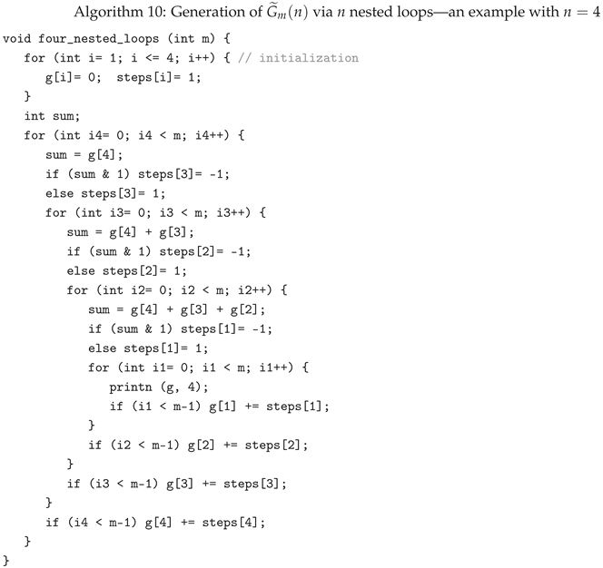
We start with an algorithm that generates this Gray code via n nested loops. It is easy to reverse the loops in Algorithm 3 in [11]: the first (outermost) with the n-th (innermost), the second with the -st, etc. However we propose another version based on Theorem 5 and closer to its recursive version, which is Algorithm 11. We illustrate the idea of such an algorithm by an example with nested loops—see Algorithm 10.
4.3.1. Nested Loops Algorithm.
The algorithm for generating via n nested loops uses two arrays, g and steps, each of length n, storing respectively the current vector and the steps for changing the elements of g. When steps[i] = 1, the element (coordinate) g[i] is increased by one, and when steps[i] = -1, the element g[i] is decreased by one, for . The variable sum maintains the sum of coordinates in accordance with Theorem 5, i.e., in the i-th loop sum= g[n]+g[n-1]+ ... + g[i], which determines the value of step[i-1], for . Note the role of the operators if (ik < m-1) g[k] += steps[k]; at the end of the body of the k-th loop, for . When the final value of ik is reached, the value of g[k] (which is 0 or ) remains unchanged until some other coordinate changes. Other details can be seen in the following example, as well as in the comments to the following algorithms for generating .
Proof of the correctness. We will prove that Algorithm 10 with n nested loops generates the vectors of by mathematical induction on n. The idea of the proof is visible in Algorithm 10. It is clear that for , the algorithm is correct. Assume it is correct for (for example, for ) nested loops. When we add the outermost -st loop (for instance, the fourth), it executes all n nested loops m times. In each iteration, it sequentially assigns the values to the last element g[n+1], and for each such assignment, the nested loops are executed. Each of these values contributes to the value of the variable sum and:
1) When g[n+1] is even, the algorithm operates according to Theorem 5 and Definition 3, i.e., with the same step values as for generating the vectors of . By the inductive hypothesis, this subset of vectors of is generated correctly.
2) When g[n+1] is odd, the algorithm again works according to Theorem 5 and Definition 3, i.e., with the opposite step values compared to those for generating the vectors of . In this way, it generates the vectors of and by the inductive hypothesis this subset is also generated correctly.
Therefore, all vectors of are generated correctly. □
4.3.2. Recursive Algorithms
As we said:
1) In [6], Ruskey proposes analogous algorithms that generate the mirror BRGC. He calls Algorithm 5.2 indirect, since the recursion is indirect—the two recursive functions call each other (as at Algorithm 2 in [11]). He proposes Algorithm 5.3, called direct—with one function that calls recursively itself. Ruskey formulates the Direct Gray Code Algorithm Superiority Principle: Try to develop direct algorithms whenever possible. It will make your programs more flexible and easier to analyze.
So we will consider a direct recursive algorithm, analogous to Algorithm 4 in [11]. This algorithm recursively implements the execution of n nested loops—see and compare with Algorithm 10. It supports and passes the variable p (means parity), which is analogous to the variable sum, namely p is sum & 1. It determines the value of the variable step ( or ), which changes g[h]. Here is its code.
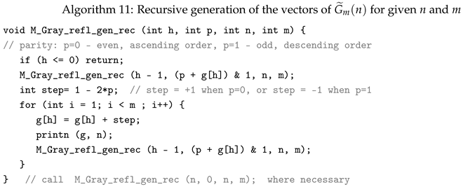
The correctness of Algorithm 11 can be proven analogously to that of Algorithm 10. Regarding its implementation, we can repeat the same thing that we said about Algorithm 4. Experimental results show that Algorithm 11 performs additional recursive calls and the same data in Table 2 are valid for it as well.
4.3.3. Nested Loops Emulation Algorithm
A short and simple non-recursive algorithm for generating the sequence or —depending on the output—is presented in [17]. It is derived after the proof of three theorems.
Here we propose a similar algorithm derived in a simpler way, we will emulate the execution of the loops in the algorithm for generating via n nested loops. The reflection in it, as in Algorithm 10, is performed according to the variable sum, so that in two successive executions of the same nested loop, the corresponding element of the array g is increased in the first execution and decreased in the second or vice versa. In other words, it is as if we have two alternative loops: the first, whose variable increases from 0 to with a step of , and the second, whose variable decreases from to 0 with a step of .
Instead of the variable sum, when emulating the execution of n nested loops, we will use a one-dimensional integer array final_vals, whose elements represent the final values of the loops: they are set to when the variable of the corresponding loop is incremented, or to 0 otherwise. Then the elements of steps take the values or respectively, used to change the i-th coordinate g[i] by that value, for . Here it is also convenient to formulate and use the rule of succession for the mirror Gray code : To obtain the next vector after the given one in the array g:
1) Scan the elements of g from left to right (i.e., g[1], g[2], etc.), looking for the first element that has not reached its final value. During the scan, swap the values: steps[i]= -steps[i] and those of their corresponding elements: if steps[i]=1, then final_vals[i]=m-1, otherwise final_vals[i]=0.
2) If the scan stops at an index , assign g[k]= g[k] + steps[k]. Otherwise, terminate, as the last vector was in the array g.
Note that this rule applies under the assumption that the arrays steps and final_vals contain the correct values corresponding to the elements of g. However, this need not always be the case, so we consider two situations, here and in Section 4.4.
First case: the arrays steps and final_vals contain the correct values. In this situation, we can construct the algorithm by sequentially applying the rule of succession. It starts with the all-zero vector and then all elements of the array steps should be set to , and these of the array final_vals should be set to . The corresponding C code is given below.
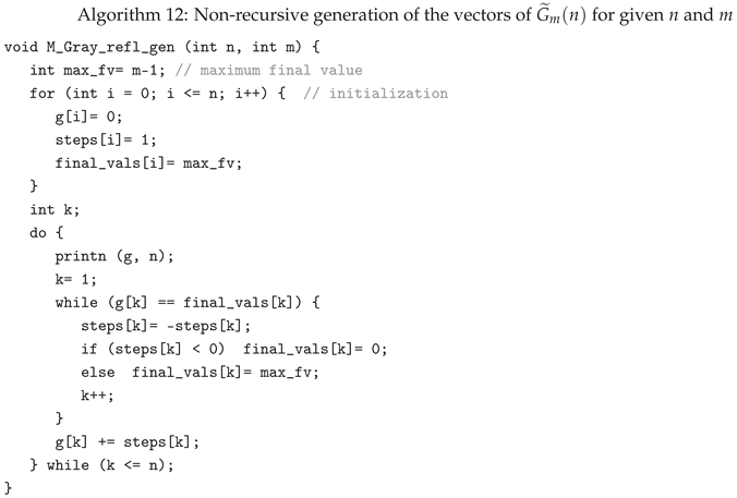
As can be seen, the algorithm continues until all elements of the array g reach their final values. Then value of k is and the main loop do ... while ends. The (inner) while loop implements the rule of succession. Although its correctness seems obvious, it can be proven rigorously by induction on n, similar to the correctness of the algorithm for generating via n nested loops.
The time complexity of the algorithm 12 is of the same type as that of Algorithm 3—they are similar and its exact estimate can be derived in the same way. The while loop is executed a total of times. For each of its executions, it performs a constant number of operations—comparisons, assignments, etc. Thus, the while loop performs a total of operations. In the body of the main loop do ... while, another operations are executed (excluding the operations in the printn function). Therefore, the total time complexity of Algorithm 12 is again and is therefore a CAT algorithm.
The results of the execution of Algorithm 11 and Algorithm 12, for are the same, they are shown in Table 5.
4.3.4. Generation of via the Transition Sequence
This topic is discussed relatively rarely in the literature, especially for non-binary Gray codes. The transition sequence for an m-ary Gray code of length n is defined as the ordered sequence of position changes from one word to the next [5,19], or in a similar manner [16,20,21]. Following [20], we denoted it by in [11], although other authors use different (often closely related) notations. Recursive definitions of are given in [16,19,20,21] and others. For m-ary reflected Gray codes, the transition sequence contains both positive and negative integers and is therefore called a mixed-sign transition sequence. Each integer specifies which coordinate should be increased or decreased by 1, depending on whether the integer is positive or negative, respectively [11,19]. In almost all sources, the codeword coordinates are numbered from right to left, for example . We note that in the mirror m-ary Gray code the coordinates are numbered from left to right, that is, , which is the mirror image of . Therefore, and have the same transition sequence.
4.4. Successor and Predecessor Functions in the Mirror Gray Code
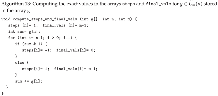
Now let us consider the second case of the rule of succession—when the correct values corresponding to the elements of g are not stored in the arrays steps and final_vals. In this situation, the task is as follows: “Given an arbitrary vector , represented by the array g. Compute (if it exists) the successor and predecessor of g”. This task admits a natural generalization: for a given integer , find the next k successors of g (if they exist or until the last vector is reached) in the sequence . Such a generalized task has applications to parallelizing the generation of all vectors of .
We cannot directly apply the ideas in the predecessor/successor functions for lexicographic order—see Algortithm 5. We need to know which coordinates of g are increasing and which are decreasing, and then we will know their final values. Following Theorem 5, we can compute the exact values for the arrays steps and final_vals that correspond to a given vector as if g had just been generated by Algorithm 12. This is the first step and its code is given below.
The second step is to compute the successor of a given vector . We can use a small part of the code of Algorithm 12, namely the while (...) loop, but simplified, since the values corresponding to g are already stored in the arrays steps and final_vals. They do not need to be changed for only one successor. However, if more successors are needed, then the code of Algorithm 12 can be adapted for this purpose. Instead of initialization, the function compute_steps_and_final_vals should be included, as well as a counter of generated vectors. Together with the variable k, they will control the main loop do ... while.
When computing the predecessor of a given vector , we need the initial values for each coordinate, not its final value. So, if any final value is , the corresponding initial value is 0, and vice versa. Thus, the initial value of g[k] is: m - 1 - final_vals[k], for . Here is the C code of these two functions.
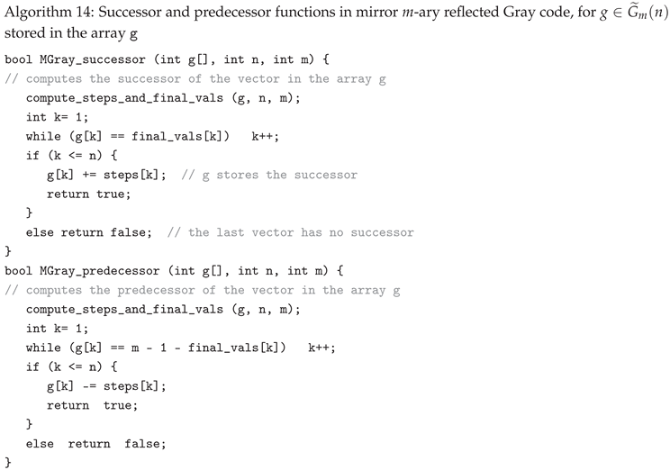
Since the function compute_steps_and_final_vals performs operations, each of the functions MGray_successor and MGray_predecessor performs a total of operations.
The ranking and unranking functions are considered in the next section.
5. Transformations Between the Orderings
Here we discuss the relationship between the considered orders, which essentially means the transformations between them. For greater clarity, they are illustrated as a directed graph (digraph) in Figure 3.
Theorem 1 states that when the vectors of are in lexicographic order, the serial number of each vector is equal to the rank of that vector, and thus they form the sequence . The transformations between a number k in a radix-m number system and the corresponding vector , whose coordinates are the digits of k, are based on the Horner rule and are referred to as ranking (of ) and unranking (of k). In Figure 3 they are labeled as and , respectively.
The basic equalities for transformations between the m-ary vectors in lexicographic order and the vectors of the m-ary reflected Gray code, are considered in [3,15,17,21,22,23]. In [11] we proved and used the following two statements.
Theorem 2 [11]. Let be a codeword in the reflected Gray code and be its sequence number. If , , , then
where and , for .
Corollary 1
[11]. Let , , , be a nonnegative integer, , and be the codeword in in the a-th row according to Definition 2. Then
where and , for .
These two statements define transformations of the vectors of in their lexicographic order and vice versa. In Figure 3 these transformations are denoted by and , respectively. This is followed by ranking a vector in lexicographic order to the corresponding integer or vice versa. Thus, as a composition of two transformations: and , the ranking and unranking functions for the m-ary reflected Gray code are obtained—see Algorithm 7 in [11].
The transformations between the lexicographic and colexicographic orders of m-ary vectors, as well as between the m-ary reflected Gray code and its mirror version, are defined by the coordinate-reversal function . As we have shown, it is an involution and is therefore drawn as a double arrow in Figure 3. Applying this function and Theorem 5 to the statements of Theorem 2 and Corollary 1 of [11], we obtain the following transformations between the colexicographic order of the m-ary vectors and the mirror m-ary reflected Gray code.
Theorem 6.
Let . Its corresponding vector in the colexicographic order of is defined by:
where , for .
Corollary 1.
Let be an arbitrary vector in the colexicographic order of . Its corresponding vector in is defined by:
where , for .
These transformations are denoted by and in Figure 3. The next step is to apply the ranking and unranking functions in colexicographic order (see Algorithm 6), based on the reversed Horner rule. They are labeled and , respectively, in Figure 3. Thus we obtain the ranking and unranking functions in the mirror Gray code as compositions and , respectively.
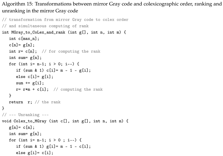
However, the computation of the rank can be simplified. The transformation from the mirror Gray code to colexicographic order and the computation of the rank in colexicographic order traverse the coordinates from right to left: n-th, -st, ..., first. Therefore, they can be combined, as shown in Algorithm 15. An analogous case occurs for the ranking function in the Gray code—see Algorithm 1 and Algorithm 7 in [11]. In both cases, the ranking can be performed without explicitly transforming to colexicographic (or lexicographic) order, since the array c (or the array a in Algorithm 7 of [11]) can be replaced by a single variable—see and compare the last two functions in Algorithm 16. Hence, the corresponding arcs are labeled as and in the digraph in Figure 3.
For the unranking in the mirror Gray code the calculations are performed in opposite directions. Therefore, the unrank in colexicographic order is first performed, followed by a transformation from the colexicographic order to the mirror Gray code, which is the composition . The same applies to the unrank in lexicographic order, followed by a transformation to the Gray code, i.e., (see Algorithm 7 in [11]).
Here is the code of the corresponding functions.
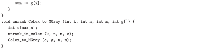
Let us consider the transformations between the lexicographic order and the mirror Gray code, and vice versa, see Figure 3. The first transformation is the composition , or equivalently , and its inverse is , or equivalently . We note that the coordinate-reversal function can be implemented while performing any of the transformations , , , or ; that is, these operations can be combined in the same manner as in the ranking function for the mirror Gray code. Consequently, each of them can be regarded as a separate transformation rather than as an explicit composition. Hence, the corresponding two arcs are added to the digraph in Figure 3 and are denoted by and .
The code of these transformations is given below. We recommend that the reader compare it with the code of the corresponding functions for colexicographic order in Algorithm 15. In addition, we propose an alternative ranking function for the mirror Gray code that follows the steps of the transformation from the mirror Gray code to lexicographic order.
We omit the consideration of the transformations between the colexicographic order and the reflected Gray code, since they are analogous to the transformations just considered. For the same reasons, they are included in the digraph of Figure 3 and are denoted as and . The code of the functions that implement them can be easily created based on the code proposed here and in Algorithm 7 in [11].
In this way, we have summarized the results of the previous sections and introduced additional relationships and transformations between the considered orders. These are illustrated in Figure 3 as a digraph that is very close to the complete symmetric digraph , with exactly two edges removed. The missing edges (should have been labeled and ) correspond to the unranking of a number from the set into an m-ary vector of length n in Gray code and in mirror Gray code. By contrast, the opposite edges, corresponding to the ranking of a vector in these orders, should be considered doubled, since ranking can be performed in two different ways. All proposed algorithms for transforming a vector from one order to another, as well as for ranking and unranking a vector or number, have the same time complexity . Furthermore, the fixed points in all these transformations are the palindromes.
6. Conclusions
Here we have examined in detail the lexicographic and colexicographic orderings of the vectors of , as well as their mirror reflected Gray code; the standard reflected Gray code is considered in [11]. We have proposed various algorithms for generating the vectors of in each of these orderings, each of which is a CAT algorithm. For each of these orderings, we have also proposed algorithms that implement the four basic functions for generating combinatorial objects, each with a time complexity of . The connections between each pair of these orderings, as well as with the set of integers , have been thoroughly investigated. The transformations between them are illustrated in Figure 3 as an almost complete symmetric digraph .
We have shown that the approach of emulating the execution of nested loops is powerful enough and leads to the creation of efficient algorithms. Our experience shows that it can be successfully applied to the generation of other combinatorial objects as well.
The mirror m-ary Gray code can have the same applications as those discussed in [11], and especially in coding theory. We hope that the remaining considerations here will also find useful applications.
Some readers may prefer only the standard m-ary reflected Gray code and not accept its mirror version. We hope that we have at least offered a different perspective and stimulated further thought in this direction.
Funding
This research was partially supported by Bulgarian National Science Fund grant number KP-06-H62/2/13.12.2022.
References
- Arndt, J. Matters Computational: Ideas, Algorithms, Source Code; Springer, 2011.
- Arndt, J. Subset-lex: did we miss an order? 2014. [Accessed 30.10.2025]. Available at:. [CrossRef]
- Knuth, D. The Art of Computer Programming, Volume 4A: Combinatorial Algorithms, Part 1; Addison-Wesley: Boston, MA, USA, 2014.
- Kreher, D.; Stinson, D. Combinatorial Algorithms: Generation, Enumeration and Search; CRC Press: Cambridge, MA, USA, 1999.
- Reingold, E.; Nievergelt, J.; Deo, N. Combinatorial algorithms. Theory and practice; Prentice-Hall: New Jersey (NJ), 1977.
- Ruskey, F. Combinatorial Generation. Working Version (1j-CSC 425/ 520). In Preliminary Working Draft; University of Victoria: Victoria, BC, Canada, 2003. [Accessed 23.11.2025]. Available at: http://page.math.tu-berlin.de/~felsner/SemWS17-18/Ruskey-Comb-Gen.pdf.
- Mütze, T. Combinatorial Gray Codes—An Updated Survey. Electron. J. Comb. 2023, 30. [Accessed 30.10.2025]. Available at: https://www.combinatorics.org/ojs/index.php/eljc/article/view/ds26/pdf.
- Savage, C. A Survey of Combinatorial Gray Codes, SIAM Review, 1997, 39, 605–629.
- OEIS Foundation Inc., The On-Line Encyclopedia of Integer Sequences. Orderings. [Accessed 30.10.2025]. Available at: https://oeis.org/wiki/Orderings.
- Bakoev, V. Mirror (Left-recursive) Binary Gray Code, Mathematics and Informatics, 2023, 66, No. 6, 559–578. [CrossRef]
- Bouyuklieva, S.; Bouyukliev, I.; Bakoev, V.; Pashinska-Gadzheva, M. Generating m-ary Gray Codes and Related Algorithms, Algorithms 2024, 17(7), 311. [CrossRef]
- Lipski, W. Kombinatoryka dla Programistów (Combinatorics for Programmers); Wydawnictwa Naukowo-Techniczne: Warszawa, Poland, 1982, 1989; ISBN 83-204-1023-1. (In Polish, Russian translation—Mir, Moskva, 1988).
- Nijenhuis, A.; Wilf, H. Combinatorial Algorithms for Computers and Calculators, (1st ed., 1975), 2nd ed., Academic Press, 1978.
- Sawada, J.; Williams, A.; Wong, D. Necklaces and Lyndon words in colexicographic and binary reflected Gray code order, Journal of Discrete Algorithms, 2017, 46-47, 25–35. [CrossRef]
- Cohn, M. Affine m-ary gray codes, Information and Control, 1963, 6, Is. 1, 70–78. [CrossRef]
- Suparta, I.N. Counting sequences, Gray codes and Lexicodes, Dissertation at Delft University of Technology, 2006. Available at https://theses.eurasip.org/theses/113/counting-sequences-gray-codes-and-lexicodes/download/. Last visited: 3.06.2024.
- Guan, D.J. Generalized Gray Codes with Applications, Proc. Natl. Sci. Counc. ROC(A) 1998, 22, 841–848.
- Er, M.C. On Generating the N-ary Reflected Gray Codes. IEEE Trans. Comput. 1984, c-33, 739–741.
- Gulliver, T.A.; Bhargava; V.K.; Stein, J.M. Q-ary Gray codes and weight distributions, Applied Mathematics and Computation 1999, 103, 97–109. [CrossRef]
- Kapralov, S. Bounds, constructions and classification of optimal codes. Doctor Math. Sci. Dissertation, Technical University, Gabrovo, Bulgaria, 2004. (in Bulgarian).
- Sharma, B.D.; Khanna, R.K. On m-ary Gray codes. Inf. Sci. 1978, 15, 31–43.
- Flores, I. Reflected Number Systems, IRE Transactions on Electronic Computers, June 1956, Vol. EC-5, No. 2, 79–82.
- Mambou, E.N.; Swart, T.G. A Construction for Balancing Non-Binary Sequences Based on Gray Code Prefixes, IEEE Trans. Inf. Theory, Aug. 2018, Vol. 64, No. 8, 5961–5969. [CrossRef]
| 1 | This problem is equivalent with generating all: (1) generalized characteristic vectors of the subsets (submultisets) of a given multiset [2]; (2) n-tuples of the Cartesian product of n sets. |
Figure 1.
The four basic function used in generating combinatorial objects.

Figure 2.
The sequence of serial numbers of the vectors of and its derivation according to Theorem 2.
Figure 2.
The sequence of serial numbers of the vectors of and its derivation according to Theorem 2.
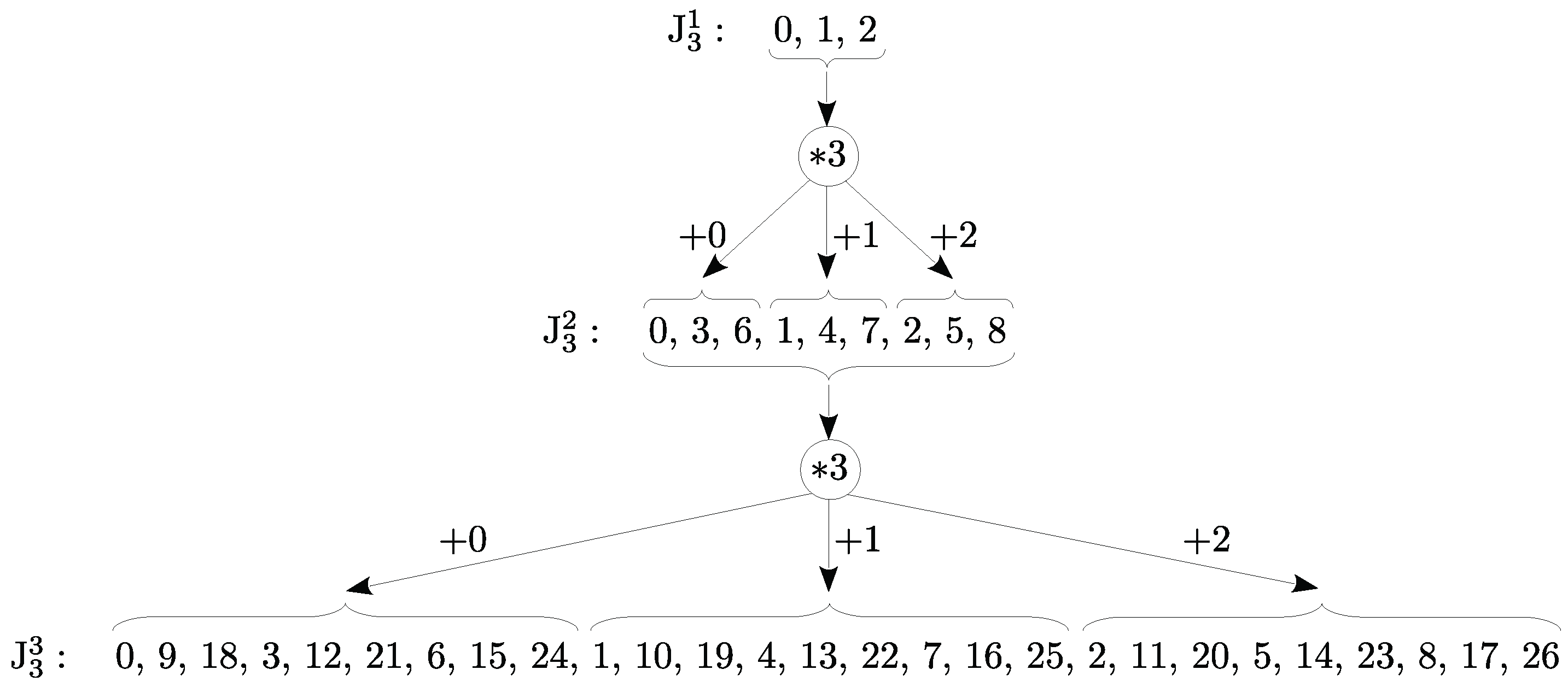
Figure 3.
Transformations between the orderings of m-ary vectors, their ranking and unranking.
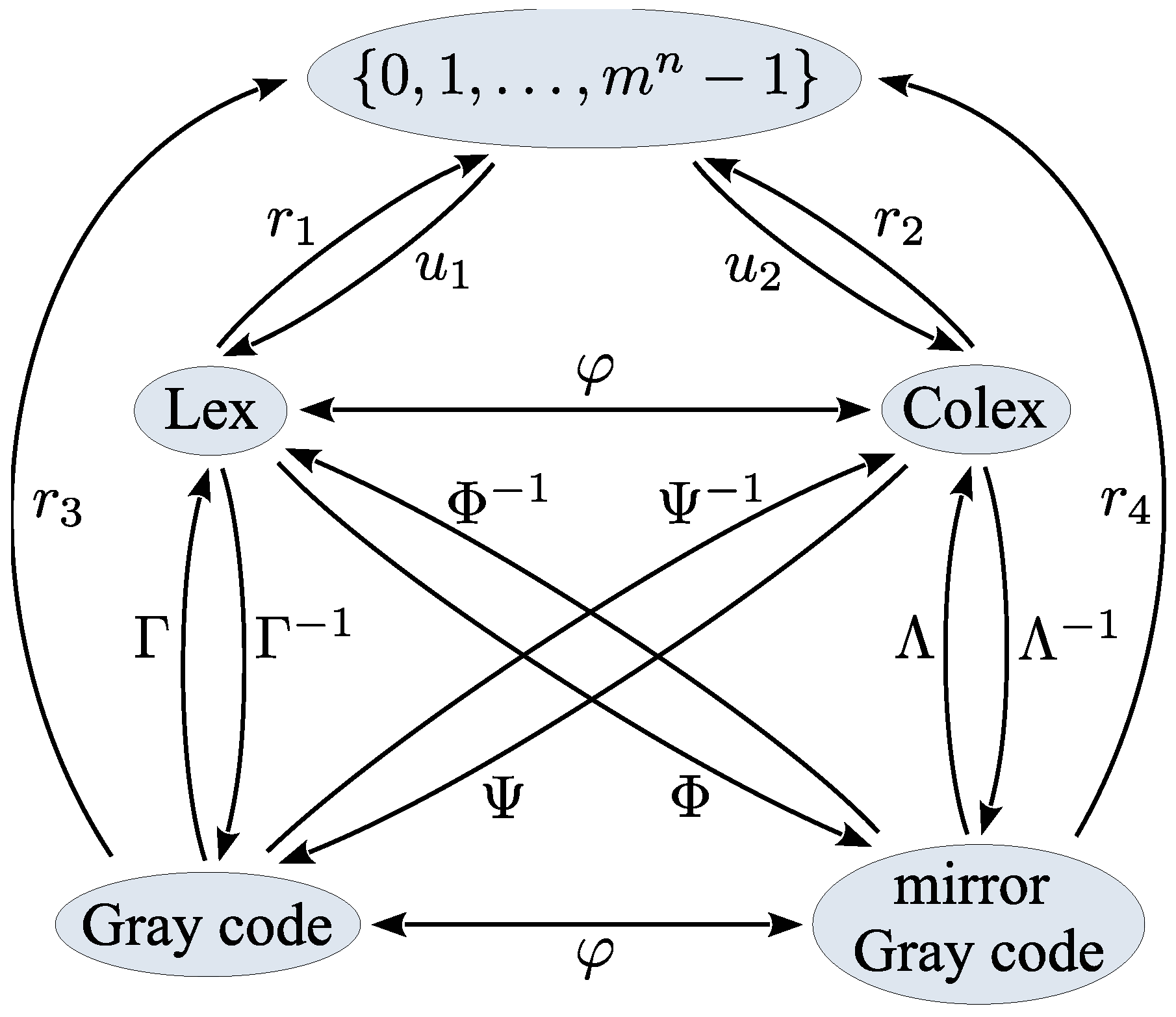

Table 1.
The vectors of in lexicographic order and their serial numbers equal to their rank.
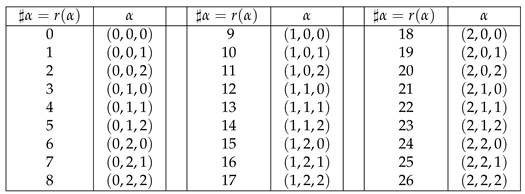
Table 2.
The percentage ratio between the number of recursive calls and the number of vectors generated.
Table 2.
The percentage ratio between the number of recursive calls and the number of vectors generated.
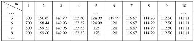
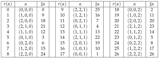
Table 3.
The vectors of in colexicographic order, their ranks and serial numbers.
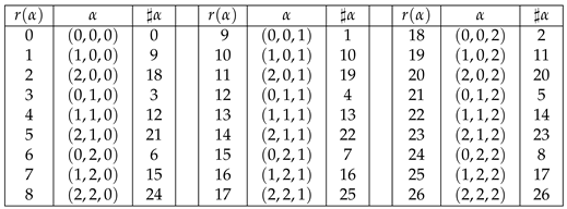
Table 4.
The vectors of , their ranks and serial numbers.

Table 5.
The vectors of , their ranks and serial numbers.
Disclaimer/Publisher’s Note: The statements, opinions and data contained in all publications are solely those of the individual author(s) and contributor(s) and not of MDPI and/or the editor(s). MDPI and/or the editor(s) disclaim responsibility for any injury to people or property resulting from any ideas, methods, instructions or products referred to in the content. |
© 2025 by the authors. Licensee MDPI, Basel, Switzerland. This article is an open access article distributed under the terms and conditions of the Creative Commons Attribution (CC BY) license (http://creativecommons.org/licenses/by/4.0/).
Copyright: This open access article is published under a Creative Commons CC BY 4.0 license, which permit the free download, distribution, and reuse, provided that the author and preprint are cited in any reuse.


