
Submitted:
18 December 2025
Posted:
19 December 2025
You are already at the latest version
Abstract
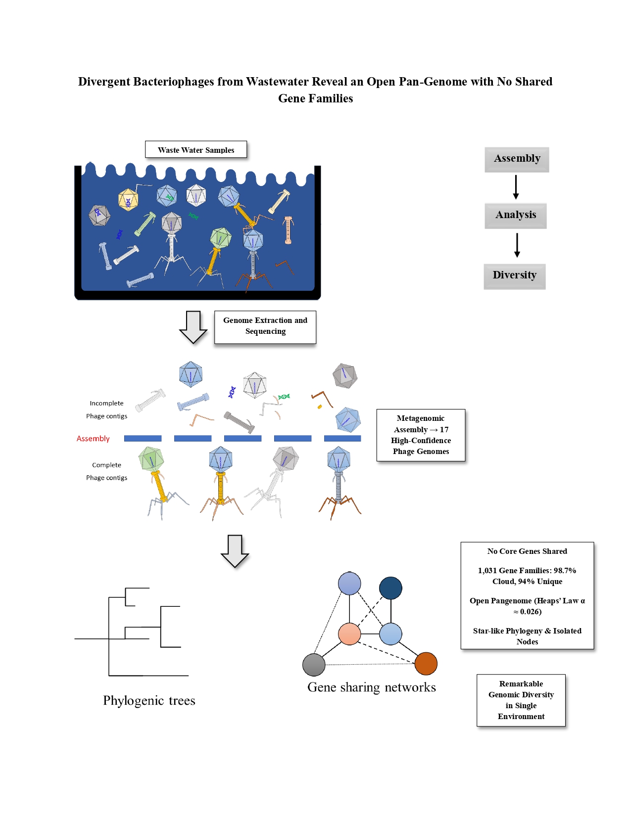
Bacteriophages, the most abundant and genetically diverse biological entities, have much of their diversity unexplored. Wastewater systems with intact microbial com-munities serve as reservoirs for diverse phages. This study recovered complete phage genomes from rural wastewater metagenomes to assess their genetic diversity. Meta-genomic sequences from six wastewater samples were assembled, viral contigs identi-fied using PHASTEST, yielding 17 high-confidence phage genomes. These were anno-tated and compared via pangenome analysis, gene-sharing networks, phylogenetic re-construction, and average amino acid identity. Heaps’ law and UpSet plots quantified pangenome openness and gene family intersections. The 17 phage genomes encoded 30–172 proteins each, sharing no core genes. Of 1,031 gene families, 98.7% were “cloud” and 94% unique, with only 13 “shell” families in >2 phages. Most shared no genes (average Jaccard similarity < 1%), 15 appearing as isolated nodes in networks. Phylogenetic trees exhibited star-like topology, reflecting distinct paths. The pange-nome was open (Heaps’ law α ≈ 0.026), with minimal overlap confirmed by UpSet, and ancestral reconstruction indicated stable genomes with occasional gains. In conclusion, bacteriophages exhibit extreme genomic diversity even in one environment, each ge-nome largely unique, highlighting the immense uncharted phage diversity and sup-porting high diversity in varied habitats.
Keywords:
bacteriophage diversity
; open pangenome
; wastewater virome
; gene-sharing network
; environmental phage genomics
1. Introduction
Bacteriophages are the most abundant biological entities on Earth, with an estimated 10³¹ particles in the biosphere [1]. Despite their ubiquity, our understanding of phage diversity remains limited. Phages have been called the “dark matter” of the biological world due to their enormous genetic diversity and many remaining secrets [2]. Rapid sequencing advances have surged new phage genomes; complete ones in public databases doubled within three years [2]. Yet, even with thousands available, they represent only a small fragment of total phage contigs diversity [1,3,4]. Strikingly, many phage genes lack homologs in current databases [5,6]. These orphan genes show how each new phage broadens the known viral gene pool. Breadth-oriented studies continuously widen the phage pangenome, offering novel genes for future work [7].
Phages also play key ecological and evolutionary roles. They drive bacterial dynamics and impact biogeochemical cycles by modulating microbial communities [8,9]. Via transduction and gene exchange, phages enable horizontal transfer among bacteria, e.g. affecting virulence and metabolism [10,11,12]. In biotechnology and medicine, phages have been invaluable from early discoveries to modern phage therapy and molecular tools [13,14,15,16]. Yet, most characterized phages stem from a small set of model systems, leaving vast biodiversity unexplored.
Environmental surveys indicate every habitat—from oceans to soil to human gut—harbors unique phages adapted to local hosts. Wastewater is particularly rich in microbial diversity, hence likely in phages infecting those microbes [9]. Urban sewage studies isolated distinct phages across host genera [1]. Environments yield phages with varied genome sizes, morphologies, and specificities [17,18]. Thus, exploring under-sampled settings is crucial for new viral lineages and innovations.
Here, metagenomic samples from rural wastewater facilities were analyzed for intact phage genomes. We hypothesized diverse microbes would yield high phage diversity, with largely unique genetic content per genome. Assembling viral contigs and identifying complete phages yielded a collection from these samples. Comprehensive comparative genomics characterized relatedness—or lack thereof—among them. This study expands environmental phage genomics, shows genomic distinctness in one setting, and assesses common/core genes. Such insights advance phage diversity and evolution, highlighting novelty from each new phage.
2. Materials and Methods
2.1. Data Collection
Metagenomic data were retrieved from BioProject PRJNA906478 (https://www.ncbi.nlm.nih.gov/bioproject/?term=PRJNA906478), encompassing rural decentralized wastewater treatment facilities in China, as part of a study conducted at Jiangnan University. These data, generated via Illumina MiSeq paired-end whole-genome sequencing (WGS) and published on November 30, 2022, were accessed from the NCBI Sequence Read Archive (SRA). The project included six SRA experiments with accession numbers SRX24547821, SRX18428665, SRX18428664, SRX18428663, SRX18428662, and SRX18428661. Datasets were imported into the UseGalaxy server for analysis. This resource provides substantial environmental data, indicating an abundance of bacteriophages with extensive genomic diversity.
2.2. Data Manipulation
FASTQ files from SRA entries were collected in UseGalaxy under unique identifiers. Trimmomatic package was applied to remove low-quality reads and adapter sequences. Contigs were assembled per sample using metaSPAdes tool [19]. Taxonomic classification of reads was performed with Kraken tool, which assigns labels based on organism-based matches [20,21,22]. Assembly outputs from metaSPAdes were subsequently classified against the viral_2020 database.
2.3. Phage Prediction and Annotation
Contigs were retained for intact bacteriophage identification. Each sample was screened for bacteriophages using the PHAge Search Tool with Enhanced Sequence Translation (PHASTEST) web tool under default settings [23]. FASTA files per sample were preserved for annotation. Pharokka was employed for open reading frame (ORF) prediction, nucleotide translation, and annotation [24]. GenBank (GBK) files were produced for each intact phage to facilitate downstream processing (see Additional file 1 for fully annotated phage genomes).
2.4. Computing Environment
Analyses were conducted on a Windows workstation utilizing Windows Subsystem for Linux (WSL) for MMseqs2-based sequence clustering [25]. Python 3.10 with Biopython 1.85 handled genome parsing and protein extraction. R 4.5.1, incorporating base R and packages including micropan, ape, phangorn, vegan, ComplexHeatmap, ggplot2, ggtree, igraph, and ggraph, managed pangenome statistics, phylogenetics, and visualization. MMseqs2 (v13-45111+ds-2) was executed within WSL or via the wsl mmseqs command from Windows; all parameters listed represent values directly supplied to MMseqs2.
2.5. Genome Parsing and Protein Extraction
GenBank records were parsed using Biopython’s SeqIO module. For each coding sequence (CDS) feature, the canonical amino-acid sequence was extracted from the translation qualifier if available. Absent translations prompted in-frame translation of the nucleotide sequence via Biopython’s codon table, ensuring a consistent fallback. Proteins were output in FASTA format with headers encoding the genome identifier, a unique index, and genomic coordinates with strand where specified. This method maintains an annotation-consistent proteome for clustering, avoiding ORF re-prediction.
2.6. Clustering Proteins into Gene Families
Gene families resembling orthologs were inferred via MMseqs2’s greedy MEM clustering. All proteins across genomes were concatenated into a single FASTA file and converted to an MMseqs database (createdb). Clustering applied a minimum sequence identity of 0.30 and alignment coverage of 0.50 in coverage mode 1, enforcing the threshold on one sequence (pipeline standard). The default greedy algorithm with three refinement iterations was utilized; sensitivity matched MMseqs2’s clustering default, equivalent to -s 5. Each protein was assigned to at most one cluster, with a representative sequence retained. A membership table of cluster representatives versus member IDs was generated for presence–absence matrix construction.
2.7. Presence–Absence Matrix and Gene Partitions
A binary genome-by-family matrix "M"∈{0,1}^(G×F) was assembled from the cluster membership table by marking M_(g,f)=1 if any protein from genome g belonged to family f, and 0 otherwise. From the column sums of M, gene partitions were computed using widely adopted thresholds: core genes are present in 100% of genomes; soft-core in ≥95%; shell in 15–<95%; and cloud in <15% of genomes. These categories provide a succinct description of the pangenome’s structural composition and are used subsequently to summarize gene sharing.
2.8. Definition of Pangenome Metrics
Standard metrics were computed from the presence–absence matrix for clarity. Total predicted proteins (CDS) denote annotated coding sequences per genome. Total gene families (pangenome size) indicate unique orthologous clusters across genomes. Core gene families appear in 100% of genomes; soft-core in ≥95%. Shell gene families are present in 15–<95% of genomes, while cloud gene families occur in <15%. Singletons represent families unique to one genome. Heaps’ law α quantifies pangenome openness, with α < 1 signifying an open, expanding pangenome.
2.9. Pangenome Accumulation and Openness
Pangenome and core-genome growth were assessed through permutation rarefaction with micropan. For each k=1,…,G, distinct families after sampling k genomes were averaged over 500 permutations (seed = 42), yielding the mean pangenome curve and 95% interval. The core curve similarly reflected families present in all sampled genomes per permutation. Openness was evaluated by fitting Heaps’ law to the pangenome rarefaction: P(k)≈β_0+β_1 k^α,
where P(k) is the expected pangenome size at k genomes, α is Heaps’ α, and α < 1 is interpreted as an open pangenome (continued gene discovery with additional genomes), whereas α ≥ 1 indicates a more closed repertoire.
2.10. Gene-Content Distances, Clustering, and Heatmaps
Pairwise gene-content relatedness between genomes was measured using the Jaccard distance on the rows of M. For two genomes with presence vectors , the similarity is
and the distance is . A Neighbor-Joining (NJ) tree was inferred from this distance matrix; in parallel, an UPGMA tree was generated from hierarchical clustering using average linkage. To visualize global relatedness, a heatmap of Jaccard similarity was plotted with genomes ordered by the NJ tip order so that block structure in the matrix aligns with inferred relationships.
2.11. Intersections of Shared Gene Families
To summarize combinatorial sharing beyond the capacity of Venn diagrams, presence sets were constructed for each genome. The ComplexHeatmap implementation of UpSet was used to compute and visualize the largest intersections among (“distinct” mode). Empty sets (genomes without present families under the chosen filters) were excluded before counting. Displays featured bars for set and intersection cardinalities, illustrating genome combinations with maximal shared families.
2.12. Genome–Genome Gene-Sharing Network
Beyond pairwise distances, a weighted, undirected gene-sharing network was constructed whose nodes are genomes and whose edge weights are the Jaccard similarities . To avoid a saturated graph and emphasize non-trivial sharing, edges with weights below 0.10 were discarded. The resulting graph was simplified to merge parallel edges, and Louvain community detection was used to explore mesoscale structure. A force-directed layout (Fruchterman–Reingold) provided a stable visualization in which node sizes reflect each genome’s gene-family richness (row sums of M) and edge widths scale with Jaccard weight.
2.13. Ancestral Reconstruction of Presence/Absence and Branch Dynamics
Gene-family turnover was mapped phylogenetically by reconstructing ancestral states as absent/present characters. The NJ tree was midpoint-rooted, with multifurcations resolved to bifurcating topology. Maximum-likelihood states were estimated per family under an equal-rates (ER) model using ace from ape. Probable states at internal nodes were selected via argmax of likelihood vectors. Edge traversals counted 0-to-1 transitions as gains and 1-to-0 as losses; invariant families were omitted. Gain/loss tallies per node were aggregated and overlaid on the tree with ggtree to emphasize dynamic lineages.
2.14. Proteome-Level Relatedness by AAI
Average Amino-Acid Identity (AAI) provided an alternative proteome similarity metric via reciprocal best hits (RBH) in MMseqs2. Bidirectional searches per genome pair used minimum identity 0.30 and coverage 0.50 in mode 1. Best hits per query were chosen by composite score, favoring long, high-identity alignments. RBHs were mutual best hits. Pairwise AAI was the alignment-length-weighted mean percent identity across RBHs:
This approach mitigates bias from short HSPs. Thresholds were fixed as stated, though sensitivity adjustments were optional for divergent proteomes.
2.15. Visualization and Reporting
Figures were produced at 300 dpi using ggplot2, ComplexHeatmap, ggtree, and ggraph. The full analysis—encompassing pangenome curves with 95% envelopes, Heaps’ α estimation, Jaccard heatmaps, UpSet intersections, gene-sharing network, ancestral gain/loss overlays, and AAI heatmaps/histograms/networks—was documented in an R Markdown report rendered to HTML and PDF via xelatex for precise typesetting (see Additional file 2).
3. Results
3.1. Phage Identification and Annotation
Analysis of biosamples for intact bacteriophages yielded seventeen viruses, with at least two intact phages isolated per BioSample. Phages were annotated, and their details are shown in Figure 1A. Findings revealed wide variation in predicted protein-coding capacity: individual genomes encoded 30 to 172 proteins, averaging ~66 per phage (95% CI ≈ 66 ± 17.6) (Figure 1B). For instance, phage_17 (smallest) encoded 30 proteins, while phage_10 (largest) encoded 172—nearly three times the mean. This genome size variation aligns with pan-genome gene family patterns.
3.2. Pangenome Composition and Statistics
Across the 17 phages, 1,031 distinct gene families were identified. The pan-genome featured rare, lineage-specific genes: 98.7% were “cloud” genes in ≤2 phages. Most (966 of 1,031 families, 93.7%) were unique to one genome, signaling an open pan-genome. Only 13 families (1.3%) appeared in three or more phages (“shell” genes), with the widest distribution in ≤5 phages. Thus, each genome held a predominantly unique repertoire, with limited broad sharing.
A total of 1,122 predicted proteins formed 1,031 orthologous families. Table 1 outlines pangenome composition and statistics. No families occurred in all genomes (0 core/soft-core genes), highlighting no universal set among the 17 phages. Indeed, 966 families (93.7%) were singletons per genome. The most widespread family reached only 5 phages (29%). These patterns indicate extreme diversity and minimal overlap.
3.3. Gene Content Similarity and Phylogeny
Phylogenetic trees based on gene content similarity explored phage relationships. A presence/absence Jaccard matrix of 1,031 families informed Neighbor-Joining (NJ) and UPGMA clustering. Both trees showed consistent groupings: high-overlap phages clustered, while low/no-share phages diverged. For Example phage_16 and phage_17 (~33 proteins each) formed a tight cluster, with the lowest Jaccard distance (~0.788, ~21% shared families). Phage_10 (largest) was an outlier, with near-maximal distances (Jaccard ~1.0) due to unique content. NJ and UPGMA topologies (Figure 2A, 2B) aligned, confirming robust gene-content links.
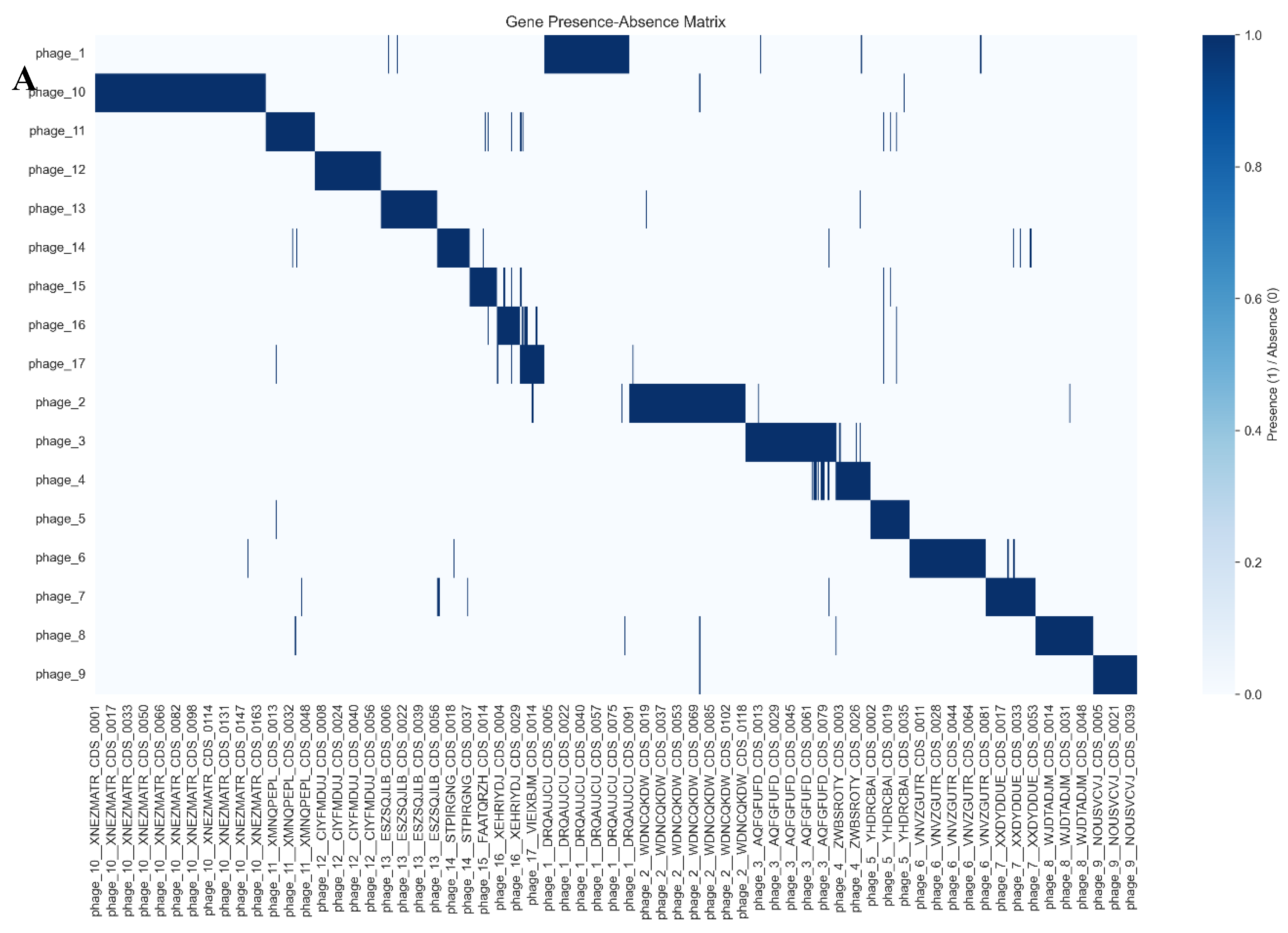
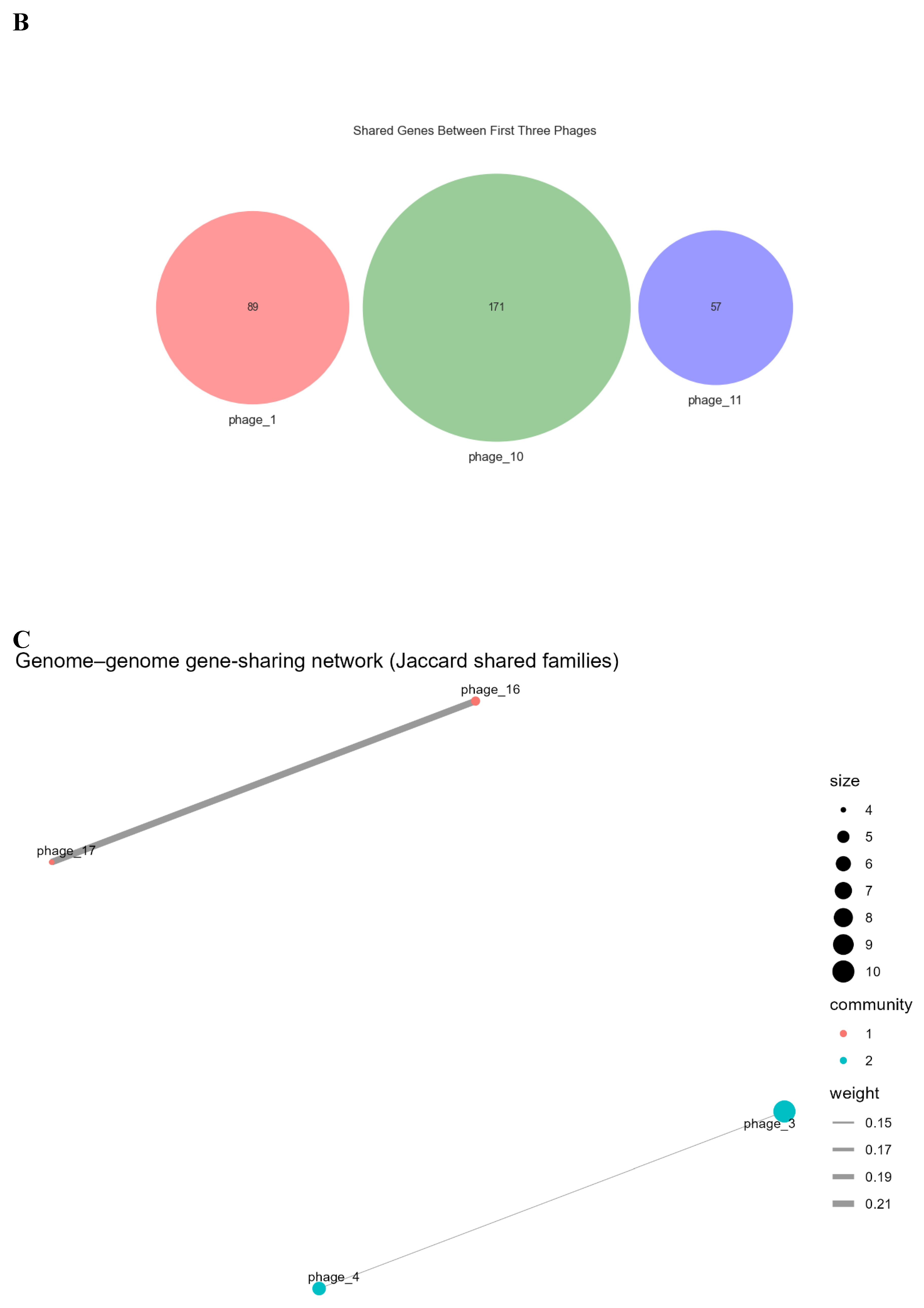
Presence/absence comparisons underscored sparse sharing. The pan-genome matrix (Figure 4A) displayed off-diagonal sparsity, confining most families to single genomes. Few shared families appeared as isolates (“shell” genes). For example phage_16 and phage_17 shared a small set of genes, matching clustering; but many pairs overlapped none. Average pairwise sharing was <1% (Jaccard similarity ~0.9%). Phage_1, phage_10, and phage_11 shared zero genes; their comparison (Figure 4B) confirmed uniqueness: 89, 171, and 57 families, respectively, with no overlaps. This illustrates individualized content, with sharing confined to small clusters and most genes private.
Pangenome accumulation analysis affirmed diversity. The mean curve (Figure 3A) rose to 1,031 families without plateauing at 17 genomes, indicating ongoing novelty per addition—indicated by low Heaps’ law α (0.026), denoting openness. Core genome dropped rapidly: after few genomes, shared families neared zero; at 17, it stayed empty, matching core absence.
Protein clustering into gene families skewed toward singletons: of 1,031 families, 966 (93.7%) were genome-exclusive, emphasizing unique genes per phage. Only 65 (6.3%) had multiple genomes, with scant breadth. Largest family in 5 phages; 4 in 4 phages; 8 in 3 phages. None exceeded 5/17 phages. This stresses limited overlap. Family presence frequencies appear in Figure 3B, stressing cloud genes dominance.
Genome pairwise similarity via binary presence–absence matrix of families yielded Jaccard distances, heatmapped in Figure 2C. Most genome pairs’ Jaccard distances neared 1.0 (no sharing), as light off-diagonals. The closest inter-genome distance were between phage_16–phage and 17 at 0.788 (~0.21 Jaccard similarity); next, phage_3 and phage_4 at 0.870 (~0.13). Few exceeded 10% similarity; ~78% pairs shared zero (distance=1.0). Uniform high-distance values in Figure 2C confirm no large gene-content clusters.
Gene content clustering analysis showed minimal grouping due to sparse sharing. The midpoint-rooted neighbor-joining (NJ) tree from Jaccard distances revealed a star-like topology with long terminal branches, indicating mostly unique gene sets (Figure 2A). Only two small clades formed: phage_16–phage_17 and phage_3–phage_4. UPGMA clustering produced identical pairings (Figure 2B). Ancestral reconstruction detected few gain/loss events per branch (usually 0–1), with the highest (13 events) on the phage_16–phage_17 clade branch, confirming that gene repertoire divergence occurs primarily between rather than within lineages.
3.4. Gene-Sharing Network and Intersections
A genome–genome network visualized higher-order sharing: nodes as phage genomes, edges for gene families (Jaccard-weighted). Threshold (edge weight ≥0.10) yielded sparse graph; sub-0.10 edges omitted, isolating most. Figure 4C shows the gene-sharing network layout: two small components, 13 singletons and no edges. Louvain detection deemed pairs communities, others solo. Nodes scaled by family count; edges by similarity. Phage_10 (171 families) is the largest isolate. Visible edges were limited to the two previously mentioned pairs, reflecting their modest shared gene families. This affirms sharing only in limited pairs, without larger clusters.
Figure 4.
Gene Sharing (binary). A. Pan-genome presence/absence matrix for phages. Rows correspond to phage genomes (labeled phage_1 through phage_17), and columns represent the 1,031 gene families (ordered arbitrarily). Blue cells indicate the presence of a given gene family in a genome, while white indicates absence. The matrix is largely devoid of shared presence across rows, evidenced by the dominance of blue along the diagonal (each phage has a unique set of gene families) and very few blue cells aligning vertically across multiple rows. Rare exceptions are highlighted by a few vertical blue streaks (examples marked by red boxes) where a gene family is present in more than one phage. These patterns demonstrate an open pan-genome with almost no universally shared genes and only a handful of gene families found in multiple genomes. B. Unique gene repertoires with no overlap among selected phages. A Venn diagram comparing gene content of three representative phages (phage_1, phage_10, phage_11). Each circle’s size reflects the number of gene families in that phage (89, 171, and 57, respectively). Notably, there are no overlapping regions between the circles – indicating zero shared gene families among these three genomes. This lack of intersection exemplifies the broader trend that many phages in the dataset do not share genes with one another. The completely disjoint gene sets of phage_1, phage_10, and phage_11 underscore the high specificity of their genetic content and the absence of any core genes common even among multiple phages. C. Genome–genome gene-sharing network. Each node represents a phage genome, with node size proportional to the number of gene families present in that phage. Edges connect genomes that share gene families, and are drawn only for Jaccard similarity ≥0.10 to emphasize non-trivial gene overlap. Edge thickness corresponds to the magnitude of the Jaccard similarity. The network reveals two small genome clusters: phage_16–phage_17 (connected by the thicker edge) and phage_3–phage_4. All other phage genomes are isolated nodes with no shared-family edge above the 0.10 threshold. Colors indicate communities identified by Louvain clustering, effectively grouping the two connected pairs separately and leaving the remaining phages as singletons. The sparsity of edges highlights the very limited gene content commonality among the phages.
3.5. Proteome-Level Relatedness and Evolutionary Dynamics
AAI distribution was heavily skewed toward zero. Of 136 genome pairs, 106 (77.9%) showed no detectable homology (AAI ≈ 0%), appearing as blank/dark cells in the heatmap (Figure 5B). Remaining pairs had AAI values of 30–70%, peaking at ~69.8% (phage_11–phage_14, n=2 proteins) and ~45.8% (phage_16–phage_17, n=12). Non-zero AAI was restricted to pairs that also clustered by gene content, demonstrating consistency between orthology presence/absence and sequence similarity measures. Overall, protein-level similarity across the phage genomes remained extremely limited (Figure 5A for network view).
UpSet analysis of 25 gene-family intersections (Figure 6) revealed that most families are exclusive to individual phages. The largest intersections were single-genome sets, led by phage_10 (168 unique families), phage_2 (112), and phage_3 (76). Multi-genome overlaps were markedly smaller; the largest comprised only 16 families shared solely by phage_16 and phage_17. Minor intersections involving three genomes contained just a few families (phage_15, phage_16, and phage_17). Overall, the plot confirmed minimal gene sharing beyond tiny clusters, with each phage possessing a substantial private gene complement, consistent with the high total family counts per genome. The set-size data show that phage_10 possesses the largest gene repertoire, while phages with smaller proteomes still predominantly contain unique genes (right side of Figure 6).
The ancestral state reconstruction of gene family gains and losses on the gene-content phylogeny (Figure 2D) shows that substantial gene turnover occurred on a few major branches. One deep ancestral node displayed the highest change (~13 gains), while another accumulated ~9 gains, indicating major innovation points in the phage evolutionary history. Large bubbles mark bursts of acquisition or loss, whereas many internal branches exhibit minimal change. This episodic pattern suggests most speciation events involved limited innovation, but some lineages experienced notable expansions, specifying branches where adaptive gene acquisitions likely occurred. This pattern matches the pan-genome finding of predominantly unique genes: most lineage splits retain existing uniqueness, while occasional bursts of gene gain or loss cause major content shifts. The ancestral reconstruction identifies branches where substantial adaptive gene acquisitions likely occurred.
4. Discussion
The analysis of 17 bacteriophage genomes recovered from wastewater metagenomes revealed an extreme level of genetic diversity among viruses in environmental context. A key finding is that these phages share virtually no genes in common, in other words, there is no detectable core genome among them. This result aligns with the expectation that phages infecting different hosts or belonging to different taxonomic families are often highly divergent in gene content. Phage genomes evolve rapidly through mutation and horizontal gene transfer as part of their arms-race coevolution with hosts [8], leading even related phages to accumulate distinct sets of genes. In the present dataset, this divergence is so pronounced that the pangenome is almost entirely cloud. Over 98% of the 1,031 gene families identified were found in only one or two phages, and 94% were singletons unique to a single phage genome. Such a skewed distribution of gene families is consistent with previous observations that many phage genes are unique or of unknown function [6,26]. It underscores the idea that each phage is genetically idiosyncratic, encoding a suite of ORFs not seen in others.
The lack of common genes across all phages is notable but not surprising. Unlike bacteria, which often share housekeeping genes, viruses have no universal marker gene present in all genomes. Even essential structural or replication genes can be so sequence-divergent or replaced by analogs that homology is unrecognizable across distant phages. The finding of zero core genes is therefore consistent with the understanding that the viral realm lacks a conserved backbone of genes connecting all members. In practical terms, by the current ICTV species demarcation criterion of ≤95% nucleotide identity across the genome [2,27,28], each of these phages would be considered a separate species. Indeed, the pairwise AAI analysis showed that most phage pairs have essentially no identifiable protein similarity, reinforcing that they share no close evolutionary relationship. The two closest pairs, phage_16 and phage_17, and to a lesser extent phage_3 and phage_4, were the only cases with non-zero AAI and a modest number of shared genes. These pairs clustered together in gene-content-based phylogenetic trees and gene-sharing networks, indicating they represent small clades of related viruses amid an otherwise star-like array of unrelated genomes. Phage_16 and phage_17, shared on the order of a dozen gene families and showed ~46% AAI, suggesting they might belong to the same broader genus or have a recent common ancestor. Similarly, phage_3 and phage_4 form a duo with a handful of genes in common. Outside these, no other phage in the collection had more than a few genes overlapping with any other.
It is instructive to compare these results with prior studies of environmental phages. A large-scale isolation from sewage demonstrated that even within one environment, phages can be extremely diverse in terms of hosts and phenotypes [1]. Similarly, a recent study by Wang et al. (2024) reconstructed over 18,000 viral operational taxonomic units (vOTUs) from wastewater treatment systems, revealing high novelty and a significant role of phages in nutrient cycling and host regulation, further supporting the extensive unexplored diversity and minimal gene sharing observed in our dataset [29]. The genomic findings of our study add to this by showing that, at the DNA level, each phage can represent a distinct genetic lineage. In essence, the wastewater sample does not harbor a swarm of closely related phages infecting one type of bacterium, but rather a mélange of phages each potentially targeting different bacterial hosts. This likely reflects the complex microbial community in wastewater; phages tend to specialize on particular bacteria, so a diverse microbial ecosystem yields a correspondingly diverse set of phage genomes. The two small clusters we observed (phage_16–17 and phage_3–4), none of which were in one sample, might indicate instances where the same or closely related bacterial hosts were present in different samples, allowing related phages in different environments. Their limited gene sharing suggests they could be different strains of a phage lineage or have diverged from a common ancestor via acquisition of different accessory genes.
Pangenome openness is an important concept for contextualizing the results. It was found a Heaps’ law exponent α ≈ 0.026, which quantitatively signifies an extremely open pangenome. In practical terms, this means that every time a new phage genome is added to the analysis, a large number of brand-new gene families appear. The pangenome accumulation curve had not begun to plateau even by the 17th genome, and indeed the curve was climbing steeply. This is consistent with Flores et al. (2024), who identified over 1,700 novel phage genomes from urban wastewater, with 80% exhibiting no shared core genes with reference databases, reinforcing that each new phage contributes unique gene families to the pangenome [30]. This trajectory indicates that the gene repertoire of phages in this environment is effectively inexhaustible, sampling additional phages would likely continue to reveal many novel genes. Open pangenomes are common in broad collections of bacteria or viruses that have high diversity. In bacteriophages, this is often taken to the extreme. In this regard, even phages infecting the same bacterial species can differ markedly in gene content, let alone phages from different families. The findings of this study exemplifies this phenomenon; the collective genome of these 17 phages is vast and mosaic, while the intersection of all 17 is essentially empty. From an evolutionary perspective, such openness reflects how phage genomes are constantly gaining and losing genes, often through horizontal gene transfer, recombination, and modular shuffling of functional gene cassettes. Prior research has shown that phages maintain diversity by exchanging flexible gene modules while sometimes preserving a core genome within a lineage [8]. Here, however, since our phages do not share a core lineage, we are observing diversity at the highest level, essentially, phages of disparate origins, rather than variations on one node.
Interestingly, the constructed gene-sharing network distilled the same insight in graphical form. With a threshold requiring at least 10% Jaccard similarity for an edge, only two edges remained. All other phages stood as solitary nodes, isolated due to negligible overlap with any other genome. This star-like network topology is characteristic of systems where most entities have unique content and few commonalities. It highlights that no larger communities or subgroups of phages exist in the dataset beyond the two small pairs, there is no evidence of a big cluster of virions sharing a host or evolutionary lineage. The network also highlighted phage_10 as a standout node due to its size and contributed the highest number of unique gene families. Phage_10’s outsized gene repertoire suggests it could be a jumbo phage or at least a relatively large-genome phage carrying many auxiliary genes. In phage ecology, larger genomes often encode additional metabolic or defense genes that can enhance the phage’s lifestyle or broaden its host range. The uniqueness of phage_10’s gene content might imply novel functions or adaptations worthy of further study. Particularly, despite its complexity, phage_10 still did not share any detectable gene with the other phages.
While sequence-based analysis shows no direct gene homology, the functionally analogous genes for capsid assembly, DNA packaging, and lysis were present, but were so sequence-divergent that they fall into different “gene families” in the clustering. Bacteriophages often achieve similar ends using proteins that, over evolutionary time, share little sequence identity. Thus, the data do not imply that these phages lack fundamental structural genes, but rather that those genes are not conserved at the sequence level across the group. From a broader standpoint, the genomic uniqueness of environmental phages suggests that every new phage genome can potentially encode novel biochemical capabilities. This is consistent with suggestions by Hatfull and others that exploring phage diversity may lead to discovery of new molecular mechanisms and tools [15]. Accordingly, the high-level divergence we observed hints that these phages likely employ different strategies to infect hosts or evade host defenses. Some may carry unique tail fiber genes for host recognition, others unusual nucleases or replication proteins. Indeed, phages are known to occasionally carry host-like genes, and in a diverse set like this, one might find evidence of genes borrowed from various bacterial pathways. Identifying and characterizing those unique genes was beyond the scope of our pangenome-focused analysis, but it remains an exciting avenue for future research.
The ancestral gene gain/loss analysis further provided insight into how phage genomes evolved in this collection. Although broad inference is difficult given the lack of close relationships, the analysis suggested an episodic pattern. In this regard, most lineages accumulated few or no new genes along their branches, but a couple of lineages underwent “burst” events of gene acquisition. Accordingly, the branch leading to the phage_16–17 clade showed a concentrated gain of around 13 gene families, possibly marking a major innovation. These bursts stand out against a background of relative stasis, where other phages changed little in gene content from their inferred ancestors. This scenario is consistent with the idea that phage genomes can undergo rare but significant exchanges, such as acquiring a plasmid or another phage’s genes during co-infection, resulting in a sudden increase in genome size and coding potential. Over longer timescales, these rare events contribute disproportionately to the expansion of the overall phage gene pool. Meanwhile, lineages without such exchanges mainly diversify via mutation in their existing genes, which would not create new gene families. The open pangenome nature observed is thus driven by those occasional leaps in gene content. It also mirrors patterns seen in some bacterial open pangenomes, where the cumulative diversity arises from a minority of lineages acquiring most of the novel genes, while others remain relatively stable.
Overall, the results support the initial hypothesis that a diverse environment like a wastewater system harbors an diverse set of bacteriophages. We see direct evidence that each phage is unique, confirming that phages from complex microbial communities overlap in genomic content unless they are very closely related. This highlights how rich the unexplored phage space is. The findings resonate with the broader literature, phage diversity research is expanding the boundaries of the viral pangenome, uncovering myriad new genes and gene combinations . Additionally, the study underscores the challenge in phage genomics of making generalizations. Each phage genome must be examined on its own merits. From an applied perspective, the novel genes within these phages could include useful enzymes like novel lysins, polymerases, or CRISPR inhibitors that might have biotechnological or therapeutic value. Expanding the sampling would also help determine whether certain gene modules recur in specific niches or whether they remain entirely unique. Additionally, we did not investigate the taxonomic family of each detected phage, which could be addressed in future studies.
There are some limitations for this study. First, the analysis was restricted to 17 phage genomes in six different bio-samples, which represents only a small subset of the wastewater virome and may not capture the full diversity present. Second, the genomes were derived from publicly available metagenomic assemblies and onlu complete genomes retained, and contigs with incomplete or chimeric sequences were discarded. Third, no host information was available, which limits the ecological interpretation of these phages, which could be addressed by determining the bacteriophages’ families. Future studies combining broader sampling, and host prediction will provide a more comprehensive picture of wastewater phage diversity.
5. Conclusions
In conclusion, this study reveals an interesting level of genomic diversity among bacteriophages in wastewater, with seventeen distinct genomes showing virtually no shared gene families and a complete absence of core genes. The pangenome is strikingly open, continually expanding with new, unique genes that highlight wastewater as a vast and largely unexplred reservoir of viral genetic novelty. Although two small clusters of related phages emerged, the majority represent independent evolutionary lineages with no detectable gene overlap—even within the same environment. These findings confirm that diverse microbial communities foster correspondingly diverse phage populations, underscoring the need to account for such genomic heterogeneity in phage therapy and environmental monitoring. Ultimately, the wealth of unique genes uncovered here reinforces the immense potential of environmental phages as sources of novel functions for ecology and biotechnology, while demonstrating the power of metagenomic and network-based approaches in illuminating the hidden complexity of viral diversity. Continued exploration of these viromes will be essential for advancing our understanding of phage evolution, taxonomy, and ecological roles.
Supplementary Materials
The following supporting information can be downloaded at the website of this paper posted on Preprints.org. File name: Additional file 1. Name: Additional file 1.zip. Description: Annotated genbank (.gnk files) data of the 17 detected bacteriophages with complete genomes. File name: Additional file 2. Name: Additional file 2.zip. Description: R markdown reports in .pdf, .html, and .log formats, indicating the prodcess of genome analyzes.
Author Contributions
Conceptualization: Alireza Mohebbi; Methodology: Alireza Mohebbi, Malihe Hamidzade, Kimia Sharifian, Seyed Jalal Kiani; Software: Alireza Mohebbi, Malihe Hamidzade; Validation: Kimia Sharifian, Seyed Jalal Kiani; Formal analysis: Malihe Hamidzade, Kimia Sharifian; Investigation: Malihe Hamidzade, Kimia Sharifian, Seyed Jalal Kiani; Resources: Alireza Mohebbi; Data curation: Malihe Hamidzade, Kimia Sharifian; Writing – original draft: Malihe Hamidzade, Kimia Sharifian; Writing – review & editing: Alireza Mohebbi, Seyed Jalal Kiani; Visualization: Alireza Mohebbi and Kimia Sharifian; Supervision: Alireza Mohebbi; Project administration: Alireza Mohebbi. All authors have read and approved the final manuscript. Co-first authors (M.H. and K.S.) contributed equally.
Funding
Not applicable.
Ethics approval and consent to participate
Not applicable.
Availability of data and materials
The datasets supporting the conclusions of this article are included within the article and in the thirdparty at NCBI’s BioProject and SRA database (https://www.ncbi.nlm.nih.gov/bioproject/?term=PRJNA906478).
Consent for publication
Not applicable.
Clinical trial
Not applicable.
Acknowledgments
During the preparation of this manuscript, the authors used Grok (developed by xAI) for limited assistance with language polishing, grammatical improvements, and minor text condensation (help in shortening abstract to meet word limits). No scientific content, data, analyses, or figures were generated by the tool. The authors have thoroughly reviewed and edited all suggestions and take full responsibility for the content of this publication.
Conflicts of Interest Statement
The authors declare that the research was conducted in the absence of any commercial or financial sponsor(s) supports and there is no a potential conflict in any financial or spiritual interests.
References
- Jurczak-Kurek, A; Gasior, T; Nejman-Faleńczyk, B; Bloch, S; Dydecka, A; Topka, G; et al. Biodiversity of bacteriophages: morphological and biological properties of a large group of phages isolated from urban sewage. Scientific Reports 2016 6:1; Nature Publishing Group, 4 Oct 2016; Volume 6, 1, pp. 1–17. Available online: https://www.nature.com/articles/srep34338.
- Zrelovs, N; Dislers, A; Kazaks, A. Motley Crew: Overview of the Currently Available Phage Diversity. Front Microbiol. Frontiers Media S.A 2020, 11, 579452. [Google Scholar] [CrossRef]
- Fremin, BJ; Bhatt, AS; Kyrpides, NC; Sengupta, A; Sczyrba, A; Maria da Silva, A; et al. Thousands of small, novel genes predicted in global phage genomes. Cell Rep [En ligne]; Elsevier B.V., 21 Jun 2022; Volume 39, 12, p. 110984. Available online: https://pmc.ncbi.nlm.nih.gov/articles/PMC9254267/.
- Benler, S; Yutin, N; Antipov, D; Rayko, M; Shmakov, S; Gussow, AB; et al. Thousands of previously unknown phages discovered in whole-community human gut metagenomes. Microbiome 2021 9:1 [En ligne]. BioMed Central 29 Mar 2021 [cité le 8 Nov 2025, 9(1), 1–17. Available online: https://microbiomejournal.biomedcentral.com/articles/10.1186/s40168-021-01017-w.
- Hatfull, GF. Dark Matter of the Biosphere: the Amazing World of Bacteriophage Diversity. In J Virol [En ligne]; cité le; American Society for Microbiology, 15 Aug 2015; Volume 89, 16, pp. 8107–10, https://journals.asm.org/doi/10.1128/jvi.01340-15. [Google Scholar]
- Pope, WH; Bowman, CA; Russell, DA; Jacobs-Sera, D; Asai, DJ; Cresawn, SG; et al. Whole genome comparison of a large collection of mycobacteriophages reveals a continuum of phage genetic diversity. Elife [En ligne]; eLife Sciences Publications Ltd, 2015; Volume 4, p. e06416. Available online: https://pmc.ncbi.nlm.nih.gov/articles/PMC4408529/.
- Hayes, S; Mahony, J; Nauta, A; Van Sinderen, D. Metagenomic Approaches to Assess Bacteriophages in Various Environmental Niches. Viruses [En ligne]. Viruses. 1 Jun 2017 [cité le 8 Nov 2025, 9. Available online: https://pubmed.ncbi.nlm.nih.gov/28538703/.
- Bellas, CM; Schroeder, DC; Edwards, A; Barker, G; Anesio, AM. Flexible genes establish widespread bacteriophage pan-genomes in cryoconite hole ecosystems. Nature Communications 2020 11:1 [En ligne]; Nature Publishing Group, 2 Sep 2020; Volume 11, 1, pp. 1–10. Available online: https://www.nature.com/articles/s41467-020-18236-8.
- Shirzad-Aski, H; Yazdi, M; Mohebbi, A; Rafiee, M; Soleimani-Delfan, A; Tabarraei, A; et al. Isolation, characterization, and genomic analysis of three novel Herelleviridae family lytic bacteriophages against uropathogenic isolates of Staphylococcus saprophyticus. Virology Journal 2025 22:1 [En ligne]. BioMed Central 2025, 22(1), 1–15. Available online: https://virologyj.biomedcentral.com/articles/10.1186/s12985-025-02710-0.
- Borodovich, T; Shkoporov, AN; Ross, RP; Hill, C. Phage-mediated horizontal gene transfer and its implications for the human gut microbiome. Gastroenterol Rep (Oxf) [En ligne]; Oxford University Press, 2022; Volume 10, p. goac012. Available online: https://pmc.ncbi.nlm.nih.gov/articles/PMC9006064/.
- Sher, S; Khan, HA; Khan, Z; Siddique, MS; Bukhari, DA; Rehman, A. Bacteriophages: Potential Candidates for the Dissemination of Antibiotic Resistance Genes in the Environment. Targets 2025, Vol 3, Page 25 [En ligne]; Multidisciplinary Digital Publishing Institute, 22 Jul 2025; Volume 3, 3, p. 25. Available online: https://www.mdpi.com/2813-3137/3/3/25/htm.
- Moura de Sousa, JA; Pfeifer, E; Touchon, M; Rocha, EPC. Causes and Consequences of Bacteriophage Diversification via Genetic Exchanges across Lifestyles and Bacterial Taxa. In Mol Biol Evol [En ligne]; cité le; Oxford Academic, 19 May 2021; Volume 38, 6, pp. 2497–512. [Google Scholar] [CrossRef]
- Dkhili, S; Ribeiro, M; Slama, K; Ben. A Century of Bacteriophages: Insights, Applications, and Current Utilization. Antibiotics 2025, Vol 14, Page 1080 [En ligne; Multidisciplinary Digital Publishing Institute, 27 Oct 2025; Volume 14, 11, p. 1080. Available online: https://www.mdpi.com/2079-6382/14/11/1080/htm.
- Sahoo, K; Meshram, S. The Evolution of Phage Therapy: A Comprehensive Review of Current Applications and Future Innovations. In Cureus [En ligne; Springer Science and Business Media LLC, 29 Sep 2024; Volume 16, 9, p. e70414. Available online: https://pmc.ncbi.nlm.nih.gov/articles/PMC11519598/.
- Hatfull, GF. Dark Matter of the Biosphere: the Amazing World of Bacteriophage Diversity. J Virol. American Society for Microbiology 2015, 89(16), 8107–10. [Google Scholar] [CrossRef] [PubMed]
- Weitz, JS; Poisot, T; Meyer, JR; Flores, CO; Valverde, S; Sullivan, MB; et al. Phage-bacteria infection networks. Trends Microbiol [En ligne]. Trends Microbiol Feb 2013 [cité le 8 Nov 2025, 21(2), 82–91. Available online: https://pubmed.ncbi.nlm.nih.gov/23245704/. [CrossRef] [PubMed]
- Naureen, Z; Dautaj, A; Anpilogov, K; Camilleri, G; Dhuli, K; Tanzi, B; et al. Bacteriophages presence in nature and their role in the natural selection of bacterial populations. Acta Bio Medica : Atenei Parmensis [En ligne]. Mattioli 1885 2020, 91 Suppl 13, e2020024. Available online: https://pmc.ncbi.nlm.nih.gov/articles/PMC8023132/.
- Ranveer, SA; Dasriya, V; Ahmad, MF; Dhillon, HS; Samtiya, M; Shama, E; et al. Positive and negative aspects of bacteriophages and their immense role in the food chain. npj Science of Food 2024 8:1 [En ligne]; Nature Publishing Group, 3 Jan 2024; Volume 8, 1, pp. 1–13. Available online: https://www.nature.com/articles/s41538-023-00245-8.
- Nurk, S; Meleshko, D; Korobeynikov, A; Pevzner, PA. metaSPAdes: a new versatile metagenomic assembler. In Genome Res [En ligne]; Cold Spring Harbor Laboratory Press, 1 May 2017; Volume 27, 5, pp. 824–34. Available online: http://genome.cshlp.org/content/27/5/824.full.
- Wood, DE; Salzberg, SL. Kraken: Ultrafast metagenomic sequence classification using exact alignments. In Genome Biol [En ligne]; BioMed Central Ltd., 2014; Volume 15, 3, pp. 1–12. Available online: https://genomebiology.biomedcentral.com/articles/10.1186/gb-2014-15-3-r46.
- Lu, J; Rincon, N; Wood, DE; Breitwieser, FP; Pockrandt, C; Langmead, B; et al. Metagenome analysis using the Kraken software suite. Nature Protocols 2022 17:12 [En ligne]; Nature Publishing Group, 28 Sep 2022; Volume 17, 12, pp. 2815–39. Available online: https://www.nature.com/articles/s41596-022-00738-y.
- Wood, DE; Lu, J; Langmead, B. Improved metagenomic analysis with Kraken 2. Genome Biol [En ligne]. BioMed Central Ltd. 2019, 20(1), 1–13. Available online: https://genomebiology.biomedcentral.com/articles/10.1186/s13059-019-1891-0.
- Wishart, DS; Han, S; Saha, S; Oler, E; Peters, H; Grant, JR; et al. PHASTEST: faster than PHASTER, better than PHAST. In Nucleic Acids Res [En ligne]; cité le; Oxford Academic, 5 Jul 2023; Volume 51, W1, pp. W443–50. [Google Scholar] [CrossRef]
- Bouras, G; Nepal, R; Houtak, G; Psaltis, AJ; Wormald, PJ; Vreugde, S. Pharokka: a fast scalable bacteriophage annotation tool. In Bioinformatics [En ligne]; cité le; Oxford Academic, 1 Jan 2023; Volume 39, 1. [Google Scholar] [CrossRef]
- Steinegger, M; Söding, J. MMseqs2 enables sensitive protein sequence searching for the analysis of massive data sets. In Nature Biotechnology 2017; Nature Publishing Group, 16 Oct 2017; Volume 35, 11, pp. 1026–8. Available online: https://www.nature.com/articles/nbt.3988.
- Jordan, TC; Burnett, SH; Carson, S; Caruso, SM; Clase, K; DeJong, RJ; et al. A Broadly Implementable Research Course in Phage Discovery and Genomics for First-Year Undergraduate Students. mBio [En ligne] 2014, 5(1), e01051-13. Available online: https://pmc.ncbi.nlm.nih.gov/articles/PMC3950523/. [CrossRef] [PubMed]
- Fu, L; Niu, B; Zhu, Z; Wu, S; Fu; Niu, B; Zhu, Z; Wu, S. Bioinformatics WL, 2012 undefined. CD-HIT: accelerated for clustering the next-generation sequencing data. LiBioinformatics: 2012, 8 Nov 2025. Available online: https://academic.oup.com/bioinformatics/article-abstract/28/23/3150/192160.
- Li, W; Godzik, A. Cd-hit: a fast program for clustering and comparing large sets of protein or nucleotide sequences. Bioinformatics [En ligne]. Bioinformatics 1 Jul 2006 [cité le 8 Nov 2025], 22(13), 1658–9. Available online: https://pubmed.ncbi.nlm.nih.gov/16731699/. [CrossRef] [PubMed]
- Wang, D; Liu, L; Xu, X; Wang, C; Wang, Y; Deng, Y; et al. Distributions, interactions, and dynamics of prokaryotes and phages in a hybrid biological wastewater treatment system. In Microbiome [En ligne; BioMed Central Ltd, 1 Dec 2024; Volume 12, 1, pp. 1–17. Available online: https://microbiomejournal.biomedcentral.com/articles/10.1186/s40168-024-01853-6.
- Flores, VS; Amgarten, DE; Iha, BKV; Ryon, KA; Danko, D; Tierney, BT; et al. Discovery and description of novel phage genomes from urban microbiomes sampled by the MetaSUB consortium. Scientific Reports 2024 14:1 [En ligne]. Nature Publishing Group 2024, 14(1), 1–14. Available online: https://www.nature.com/articles/s41598-024-58226-0.
Figure 1.
Genome Summary. A. Predicted protein counts per phage genome. A lollipop chart showing the number of protein-coding genes in each of the 17 phage genomes (points), sorted from smallest to largest genome. The dashed line indicates the mean genome size (66 proteins) with the 95% confidence interval. Genome sizes vary over a 6-fold range (30 to 172 proteins), highlighting considerable heterogeneity in coding capacity among the phages. This variation provides the context for pan-genome analyses, as larger genomes contribute many unique gene families. B. Genome features of the analyzed phages. (Top left) Distribution of genome sizes (kb), shown as a boxplot with individual genomes overlaid. (Top right) Distribution of predicted open reading frames (ORFs) across genomes. (Bottom left) Correlation between genome size and predicted ORFs, showing a strong positive linear relationship. (Bottom right) Relationship between genome size and GC content (%) modeled with a smooth curve, highlighting variability in GC% across different genome sizes.
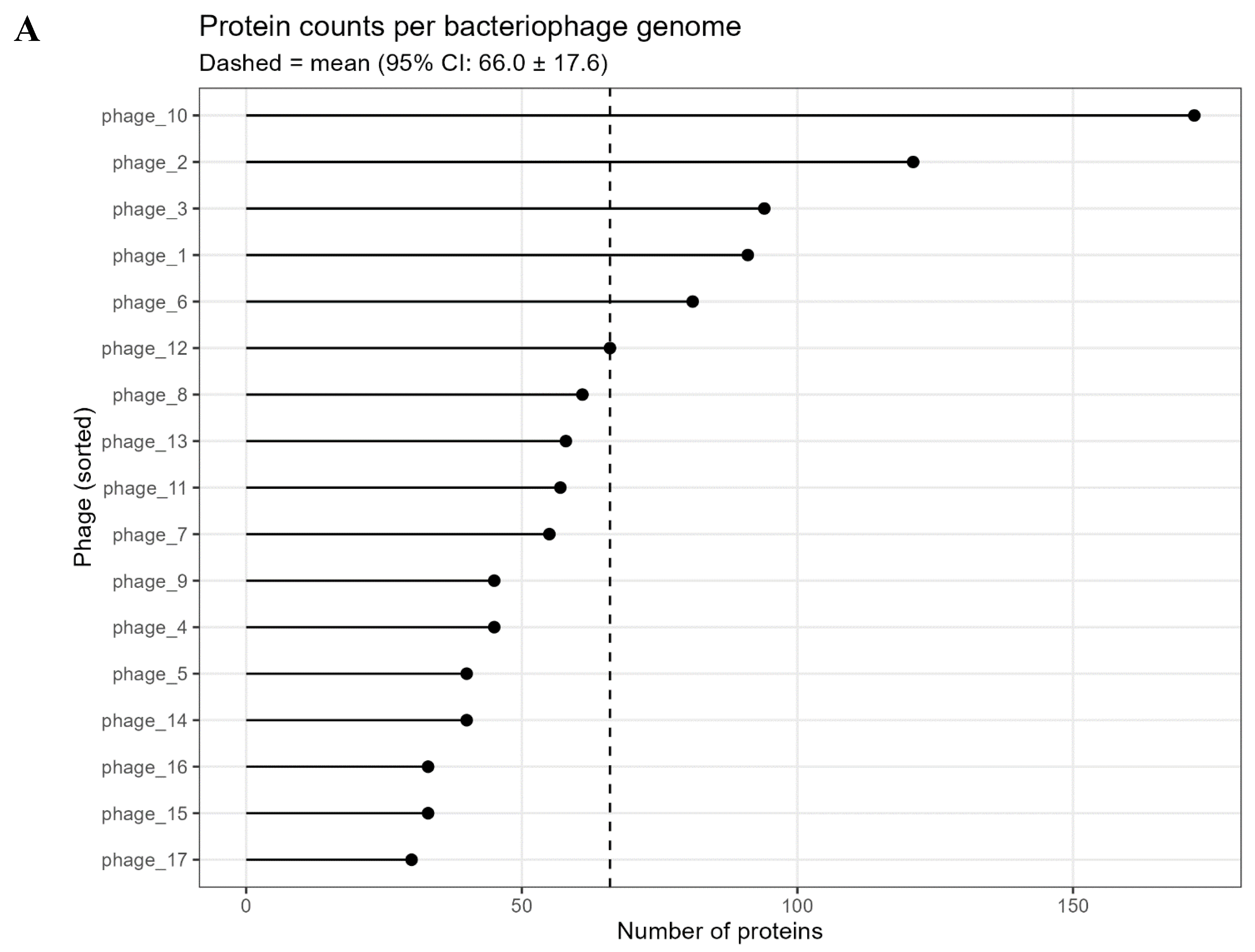
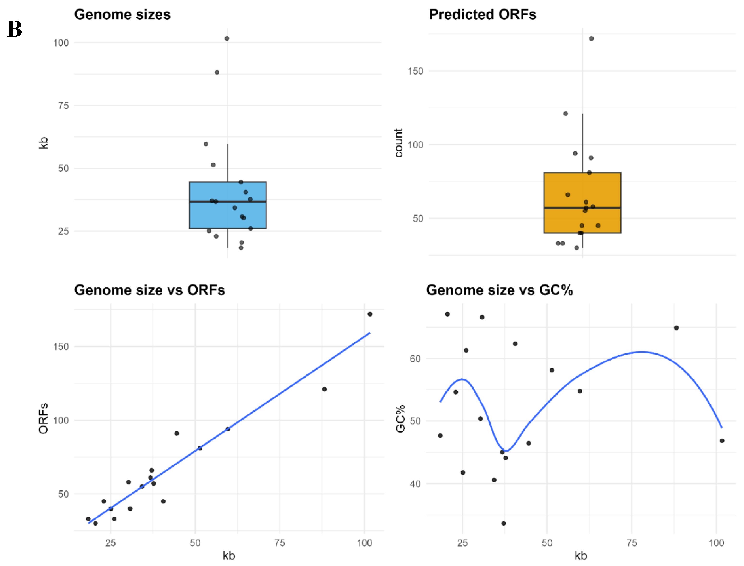
Figure 2.
Gene-content phylogeny (Neighbor-Joining at top and UPGMA bottom)and Clustering. A. An unrooted NJ tree based on Jaccard distances between phage gene repertoires. Branch lengths reflect gene content dissimilarity. Phages that cluster together (adjacent in the tree) share more gene families. Notably, small-genome phages 16 and 17 branch as closest neighbors, indicating their gene sets overlap substantially. Phages 3 and 4 also cluster, consistent with their moderate gene sharing. In contrast, phage_10 is isolated on a long branch, highlighting its high divergence (it shares virtually no genes with others). The NJ analysis thus groups phages by gene content similarity, revealing discrete clades of more closely related genomes. B. A UPGMA dendrogram built from the same Jaccard distance matrix of gene presence/absence. The overall clustering pattern mirrors that of the NJ tree, with the same major groupings observed. Phages 16 and 17 again form a distinct cluster, and phages 3 and 4 group together similarly. The consistency between UPGMA and NJ trees suggests that these relationships are robust. Minor differences in branch lengths or order are due to the clustering algorithm, but no fundamentally new groupings appear. Both methods underscore the high level of gene content divergence among the phages, as evidenced by the long branches separating most clusters. C. Heatmap of pairwise gene-content distances among the 17 phage genomes. Jaccard distance (1 − Jaccard similarity) is shown for each genome pair. Genomes are ordered according to a neighbor-joining tree derived from these distances, so that closely related phages appear adjacent. The matrix is shows minimal shared gene content). Notably, two darker off-diagonal cells are visible, one corresponds to the phage_16–phage_17 comparison, and another to phage_3–phage_4, indicating these pairs have the highest gene content. D. Ancestral gene-family gain/loss reconstruction on the phage phylogeny. A phylogenetic tree of the 17 phages is shown with internal nodes annotated by the number of gene families gained (blue) or lost (red) along each branch (inferred by maximum likelihood). Circle sizes are proportional to the total number of changes (gains + losses) at that node. Most branches have zero or few changes (no circle or very small), indicating relative gene content stasis. However, a few ancestral branches stand out with large circles – for example, one node (marked with an arrow) shows 13 gene gains, and another shows ~9 gains. These results suggest that while gene content evolution is generally conservative, there have been episodic bursts of gene acquisition in certain lineages, which contributed significantly to the divergence in phage gene content.
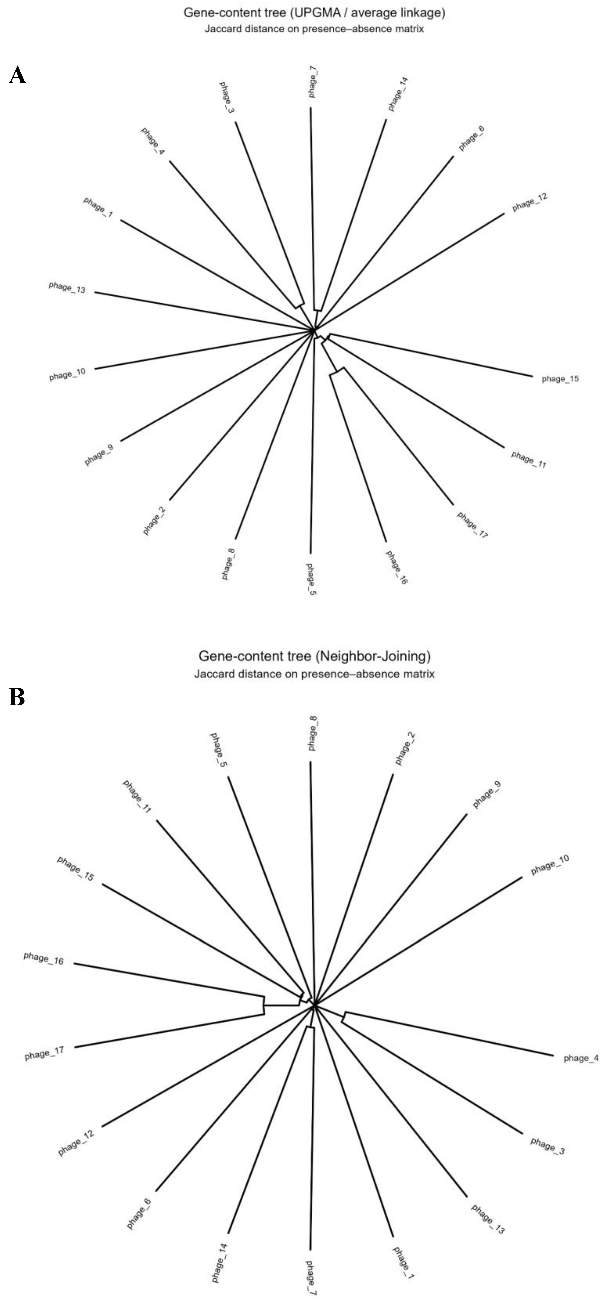
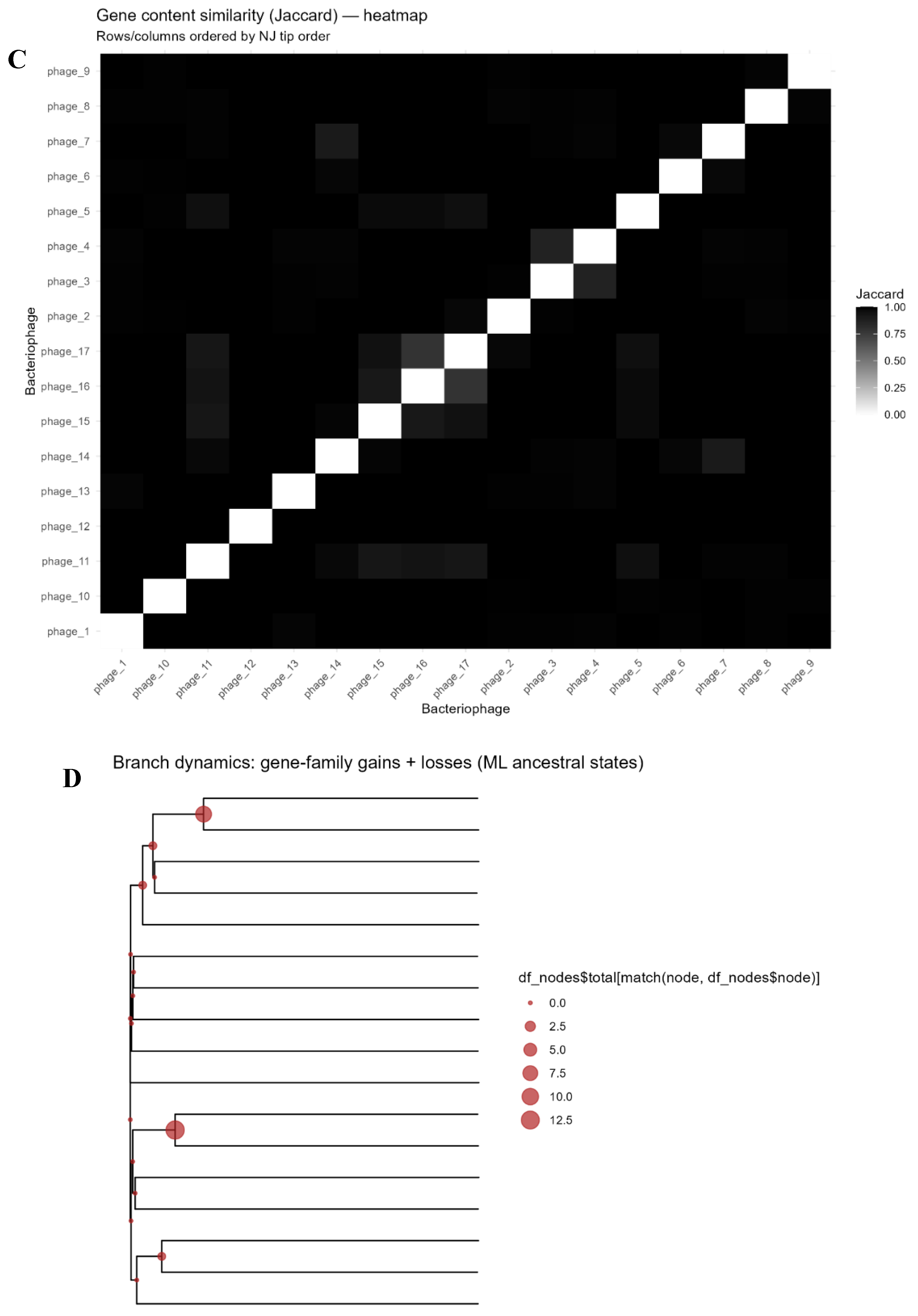
Figure 3.
Pangenomic Openness. A. Pangenome accumulation curves for the intact phages. The total number of gene families (pangenome, teal line) and the number of core families (present in all genomes, red line) are plotted as a function of genomes sampled, with shading indicating the 95% confidence interval across 500 random genome addition permutations. The pangenome size shows a steady increase, reaching 1030 families after all genomes are included, while the core genome size rapidly declines toward zero and remains essentially zero beyond 5 genomes. The non-saturating pangenome curve and vanishing core indicate an open pangenome (consistent with Heaps’ law exponent α ≈ 0.026). B. Composition of the phage pangenome by gene frequency category. A pie chart illustrates the proportion of gene families that are core (present in all genomes, 0%), soft-core (present in ≥95% of genomes, 0%), shell (present in 15–<95% of genomes, 1.3%), and cloud (present in <15% of genomes, 98.7%). The cloud segment dominates, reflecting that almost all gene families are found in only one or a few phages. Shell families constitute a negligible fraction, and no universal core genes were identified among these phages.
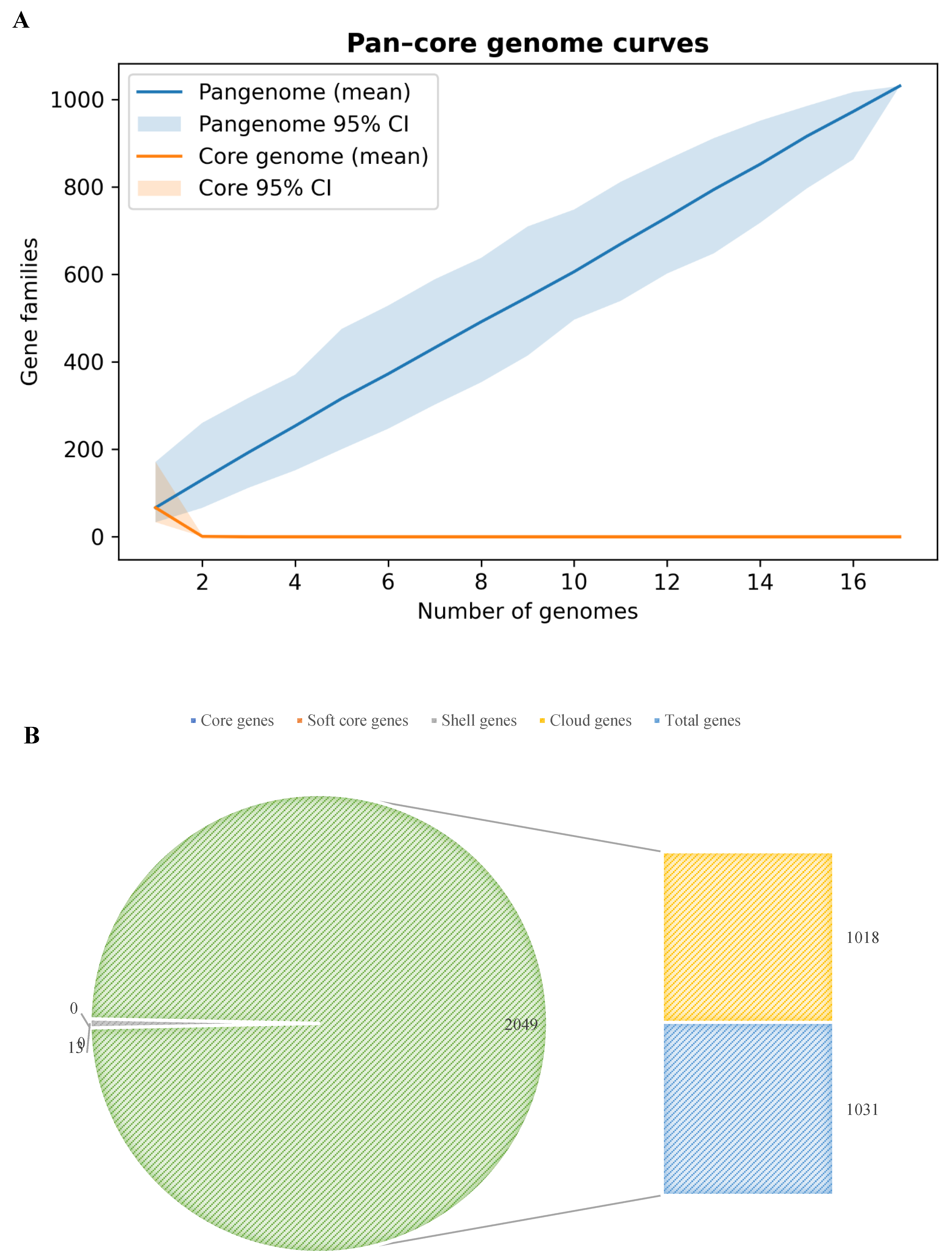
Figure 5.
Pairwise AAI Analysis of 17 Phage Genomes. A. Network of AAI Similarities. A network visualization where nodes represent phages and edges indicate AAI values above a threshold, emphasizing connected components. The network highlights sparse connections, with notable edges between phage_16–phage_17 and phage_3–phage_4, consistent with their gene content similarities. Node sizes reflect the number of gene families per phage, and edge thickness corresponds to AAI similarity strength. The sparsity of edges reinforces the limited protein-level commonality among the phages. B. Heatmap of Pairwise AAI. Each cell shows the average amino-acid identity (AAI) as a percentage between proteins of two genomes, calculated from reciprocal best-hit pairs. Dark purple/black indicates no significant shared proteins (AAI ~0%), while brighter colors (yellow/green) indicate higher identity levels. Most genome pairs have AAI = 0%. A few pairs show low-to-moderate AAI: for instance, phage_16 vs phage_17 (≈46% AAI) and phage_11 vs phage_14 (≈70% AAI) appear as the brightest cells off the diagonal. These correspond to the same genome pairs that showed the closest relationships in gene content. The heatmap underscores that protein-level similarity between these phages is minimal in most cases, consistent with their divergent gene sets.
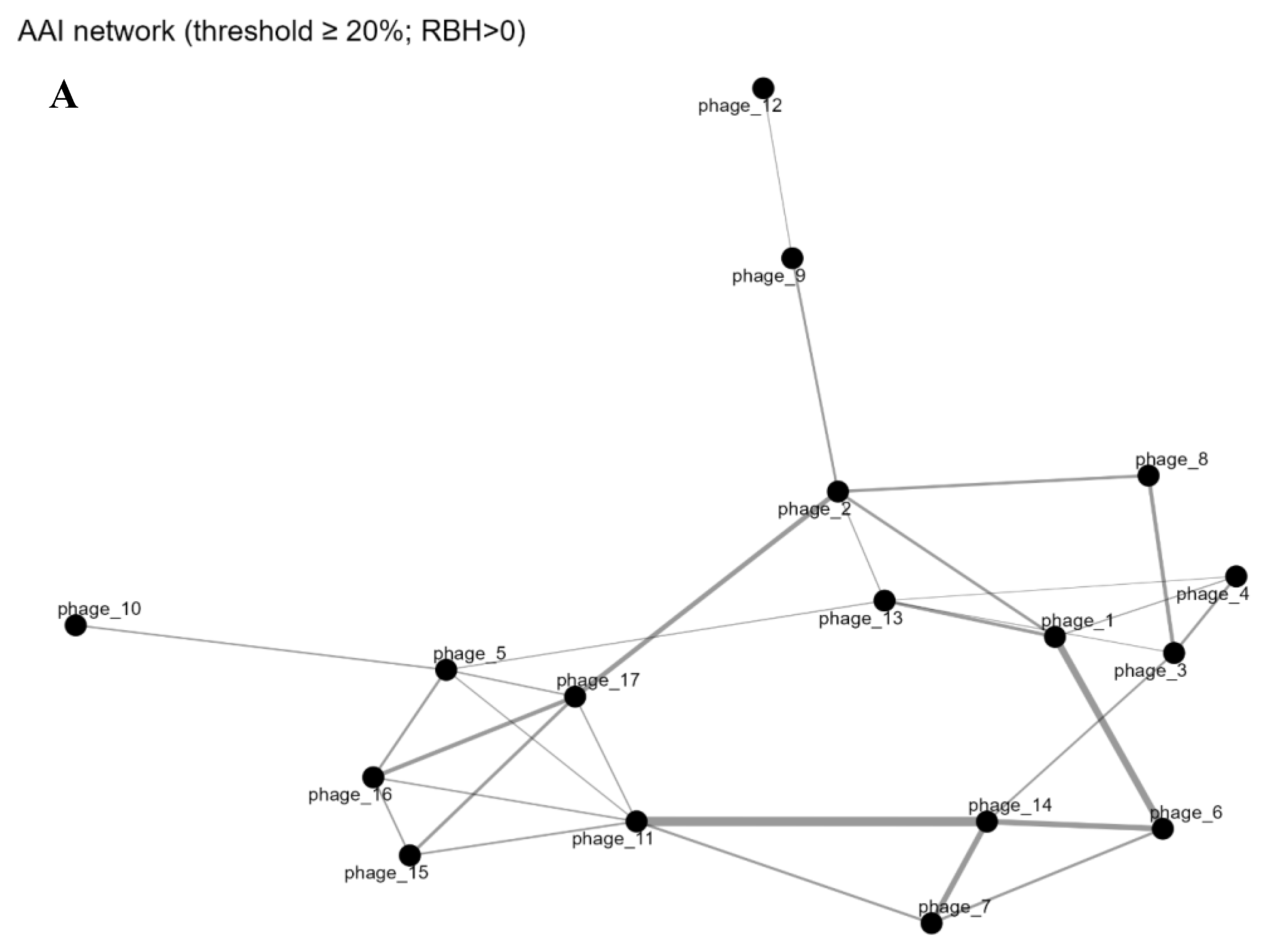
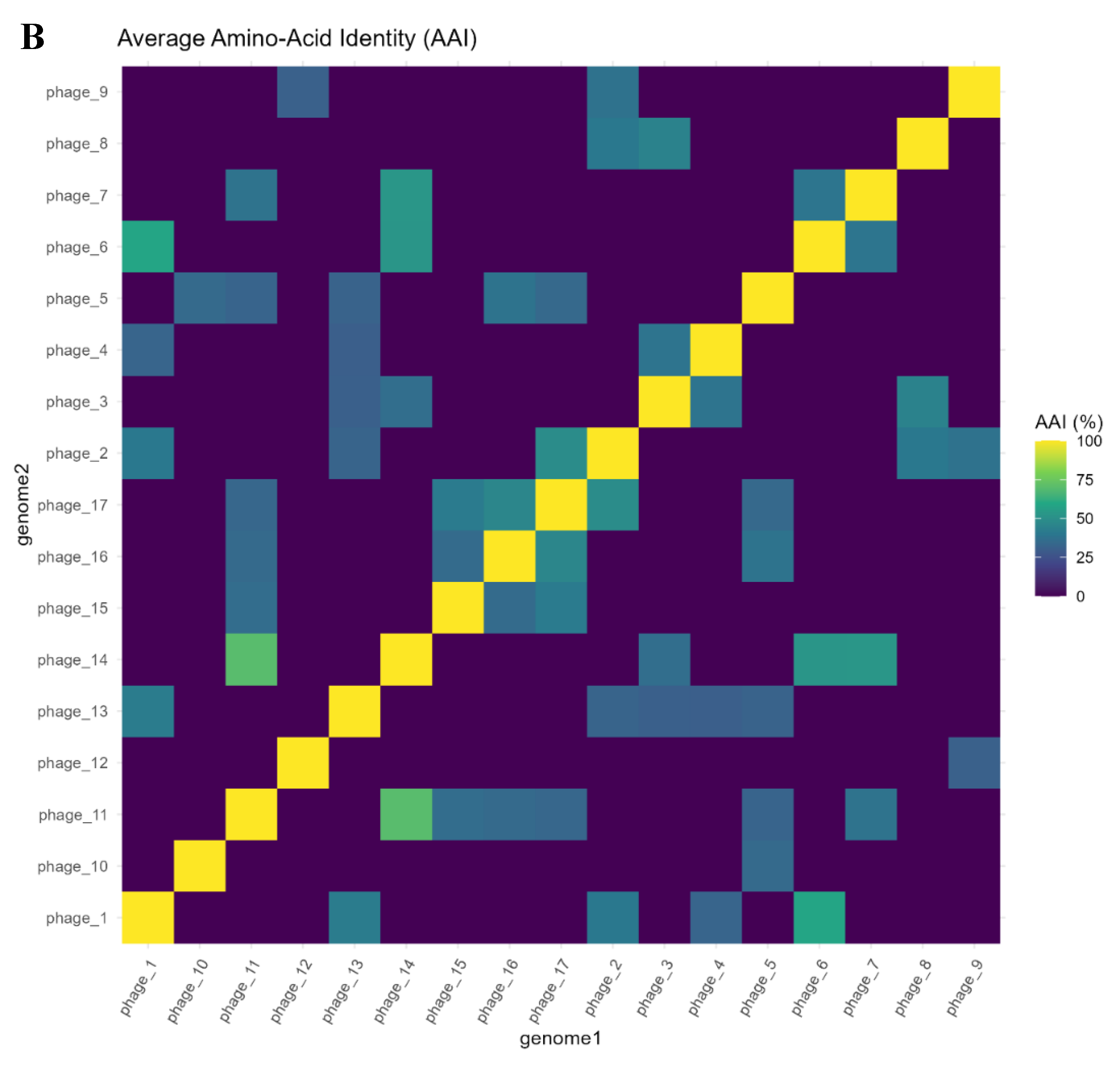
Figure 6.
UpSet plot of shared gene families among the phages. The matrix at bottom indicates specific combinations of genomes (black dots connected by lines), and the vertical bars above show the number of gene families in the intersection of those genomes’ gene sets. Only the 25 largest intersections are shown. The tallest bars correspond to gene families unique to individual phages, single-dot intersections, with phage_10, phage_2, and phage_3 having the largest unique sets (bar heights 168, 112, 76 respectively). Far fewer gene families are shared by multiple phages. Notable smaller intersections include the set of families common to phage_16 and phage_17 (bar ≈16) and a set shared by phage_15–phage_16–phage_17. The horizontal bar chart on the right shows the total number of gene families present in each phage, which corresponds to each phage’s genome gene count. This plot highlights that most gene families are genome-specific, and only very limited overlaps exist between even the most closely related phages.
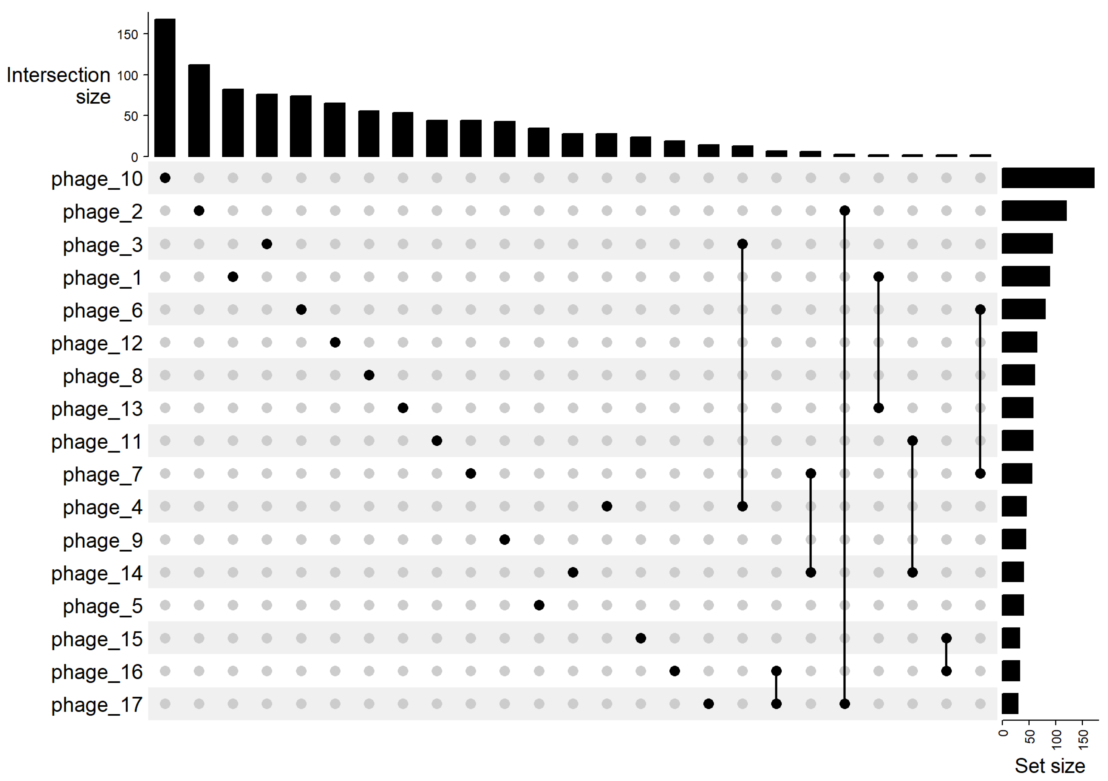

Table 1.
Summary of pangenome statistics for the 17 bacteriophage genomes analyzed. Percentages for gene family categories are relative to the total number of gene families. The Heaps’ law α parameter (with α < 1 indicating an open pangenome) is shown to quantify pangenome openness.
Table 1.
Summary of pangenome statistics for the 17 bacteriophage genomes analyzed. Percentages for gene family categories are relative to the total number of gene families. The Heaps’ law α parameter (with α < 1 indicating an open pangenome) is shown to quantify pangenome openness.
| Metric | Value |
|---|---|
| Number of phage genomes | 17 |
| Total predicted proteins (CDS) | 1122 |
| Total gene families (pangenome size) | 1031 |
| Core gene families (present in 100% genomes) | 0 (0%) |
| Soft-core gene families (present in ≥95% genomes) | 0 (0%) |
| Shell gene families (present in 15–<95% genomes) | 13 (1.3%) |
| Cloud gene families (present in <15% genomes) | 1018 (98.7%) |
| Singleton gene families (unique to 1 genome) | 966 (93.7%) |
| Heaps’ law α (pangenome openness) | 0.026 (Open) |
Disclaimer/Publisher’s Note: The statements, opinions and data contained in all publications are solely those of the individual author(s) and contributor(s) and not of MDPI and/or the editor(s). MDPI and/or the editor(s) disclaim responsibility for any injury to people or property resulting from any ideas, methods, instructions or products referred to in the content. |
© 2025 by the authors. Licensee MDPI, Basel, Switzerland. This article is an open access article distributed under the terms and conditions of the Creative Commons Attribution (CC BY) license (http://creativecommons.org/licenses/by/4.0/).
Copyright: This open access article is published under a Creative Commons CC BY 4.0 license, which permit the free download, distribution, and reuse, provided that the author and preprint are cited in any reuse.


