
Submitted:
18 December 2025
Posted:
19 December 2025
You are already at the latest version
Abstract
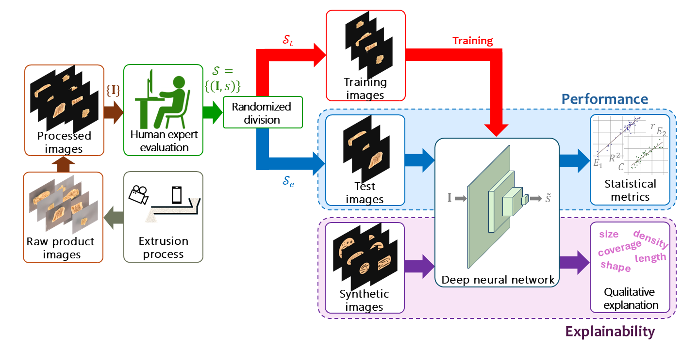
Automation of the plant-based meat extrusion process requires a scheme to provide quantitative estimates of output fibrosity, which must be carried out online and in real-time. A novel machine learning regression model for this purpose, is proposed in this article. A deep neural network that was originally trained for image classification, was extended to provide quantitative fibrosity estimates. Relevant layers of the network were retrained using real-world laboratory data. Plant-based meat or textured vegetable protein products with varying fibrous microstructures were obtained using different ingredient formulations and process conditions on a pilot-scale twin screw extruder with in-barrel moisture range of 29.2-40.9% (wet basis). Images of extruded plant-based meat products were collected to serve as sample inputs. An experiment was devised, where image samples were randomly presented to two expert human subjects, who provided as feedback, fibrosity scores lying within the interval [1, 10]. Statistical metrics were adopted to evaluate the performance of the trained network. It was found that the network performed significantly better when trained separately with feedback scores of each individual subject, than with the combined scores, indicating that it was able to capture nuances of a subject’s perception. Another study was directed at the explainability of the network’s estimations. Using standard software, a set of synthetic images of varying shapes and sizes were created as inputs to the network. Interpretations of its output scores indicate that the network’s estimates were based on features relevant to porosity and fibrosity, while not influenced by extraneous ones.
Keywords:
plant-based meat
; extrusion
; fibrosity
; deep neural network
; regression
; convolution layer
; residual network
; explainability
1. Introduction
Extrusion is a common method for producing texturized vegetable proteins (TVP) or plant-based meat, involving transformation of plant derived proteins into fibrous, meat-like structures through the combined effects of heat, pressure, shear, and moisture. This technology is valued not only for its ability to replicate the texture of meat, but also for its potential to deliver environmentally sustainable, high protein foods. Diverse protein sources, such as soy, pea and hemp, have been used for TVP products, which underscores the adaptability of the extrusion process (Webb et al., 2020; Rajendra et al., 2023; Guerrero et al., 2024).
Product microstructure, especially the development of meat-like fibers, is a key parameter that influences the textural signature including mechanical strength, chewiness, and springiness (Hong et al., 2022). The degree of fibrousness or fibrosity of TVP products is often evaluated subjectively from product images (Flory et al., 2023; Lyu et al., 2023; Rajendra et al., 2023; Plattner et al., 2024; Esbroeck et al., 2024). An objective means for characterizing fibrosity can be extremely useful in developing better structures and textures, and also in process control applications, which is the underlying goal of this research.
Research has just begun on objective measurement of microstructural features of TVP. Analytical methods for assessing plant-based meat analogues were reviewed by McClements et al. (2021), including microstructure analysis using computer vision (Hough transformation) for obtaining a fiber index value. An automated image analysis method (Fiberlyzer) was developed to quantify visual fibrousness in plant-based meats, demonstrating strong correlations between computed fiber scores and expert panel evaluations (Ma et al., 2023). This work illustrates how computer vision combined with machine learning can provide objective, standardized, and scalable assessment of fibrous structures, reducing reliance on subjective human evaluation in extrusion-based product development. In another study (Li et al., 2023) a computer vision–based laser transmission method was proposed to quantify the degree of orientation in fibrous foods using extruded jerky as a model system. This non-destructive technique was shown to reliably capture structural alignment, a feature closely associated with mechanical texture and consumer acceptance, and it offered a more objective alternative to traditional visual inspection. The relationship between structural and mechanical anisotropy in plant-based meat products has been examined (Zink et al., 2024). This study draws on small- and wide-angle X-ray scattering and scanning electron microscopy, demonstrating that higher protein content and controlled processing conditions promoted fibrous alignment and mechanical strength, with microstructural anisotropy indices emerging as robust quantitative markers of product quality. More recently, an artificial intelligence and machine learning based process modeling approach combined with computer vision to evaluate microstructural features of plant-based meat was employed to develop an integrated framework for predicting TVP fibrosity scores from extrusion parameters to support real-time process control and optimization (Bagheri et al., 2025).
A deep neural network (DNN) – such as that proposed in this research, is a machine learning model that is roughly organized in the manner of the human cortex (Goodfellow et al., 2016). It consists of several layers of array processing. The first layer (input layer) acquires the DNN’s input, which is passed onto the next “hidden” layer. Each hidden layer in the DNN receives an input array from its immediately preceding layer and obtains an intermediate output that passes its output on to next layer. After several layers of processing, the DNN’s last layer (output layer) produces the output of the DNN. The DNN’s internal parameters can be iteratively optimized by means of a learning algorithm. Classification and regression are the two broad categories of supervised learning. In classification tasks, the DNN produces discretized outputs, while in regression, the outputs are continuous quantities. Since this research pertains to a regression task; the outputs of the proposed DNN are real quantities between 1 and 10, that represent estimated fibrosity scores from plant-based meat product images as its inputs; products with different scores leading to varying textural attributes ranging from soft to chewy.
Recent years have witnessed an explosive growth in the popularity of DNNs. They have been highly successful in a wide variety of applications such as home automation (Al-Ani and Das, 2022), agriculture (Badgujar et al., 2023a), large language models (Long et al., 2025), cybersecurity (Sarker et al., 2021), automated vehicles (Liu et al., 2025), automated traffic networks (Aziz and Das, 2023), defense (Gomes et al., 2024), blockchains (Shafay et al., 2025), and robotics (Tang et al., 2025). DNNs have been applied to various food related image classification tasks, such as for the evaluation of fish quality (Wu et al., 2025; Siricharoen et al., 2025), predicting soluble solid content of sweet potato (Ahmed et al., 2024), classification of tea leaf samples (Guo et al., 2024), rice classification (Razavi et al., 2024; Wang et al., 2023), and for crack detection in wheat kernel images (Wang et al., 2023). Significant amount of research attention is being directed at gleaning coherent explanations on DNNs which are inherently black box models (Vonder Haar et al., 2023, Ibrahim and Shafiq, 2023).
Residual networks (ResNets) are a class of DNNs that were first proposed for image classification (He et al., 2016). ResNets with 18, 34, 50, and 150 number of layers were considered. A unique feature of ResNets is the presence of residual connections, which allow hidden layers to deliver outputs simultaneously to two downstream layers. Due to these residual connections, ResNets were shown to consistently outperform traditional DNNs with up to 1000 layers. Theoretical treatment provides further insights for the better performances of ResNets (Wu et al., 2019; He et al., 2020). They have been applied in a wide range of computer vision applications (Shafiq and Gu, 2022; Sharma and Guleria, 2022). ResNet architectures have been adopted for food related image processing. Eighteen layered ResNets (ResNet-18) have been considered for such applications (Wang et al., 2023; Wang et al., 2024; Hernansanz-Luque et al., 2026). ResNets with 18, as well as 34 layers have been used (Gao et al., 2024). Larger ResNets with 50 layers have been proposed elsewhere (Senapati et al., 2023; Zahisham et al., 2020). In all these cases, the ResNet was used for classification.
In this research, a ResNet-18 model that had been pre-trained for image classification (Martinez et al., 2017) was suitably modified for regression. An additional output layer was incorporated for this purpose, while the input layer was extended to handle larger images. A few layers of the original ResNet-18 were retrained for regression using data collected for this study.
The following section provides further details into the data collection and treatment methodology, as well as the modified ResNet model proposed in this study.
2. Materials and Methods
2.1. Generation of Texturized Vegetable Proteins Products
Three fava bean concentrate (45%) based formulations, each containing soy protein concentrate (11%) but different sources of complementary plant proteins (44%), viz., pea protein isolate, soy protein isolate or wheat gluten, were extruded under different processing conditions to generate TVP products with varying fibrous microstructures. The protein content of faba bean concentrate (Ingredion, Westchester, IL, USA) and soy protein concentrate (ADM, Quincy, IL, USA) were 60% and 72%, respectively, while that of pea protein isolate (Puris, Minneapolis, MN, USA), soy protein isolate (ADM, Quincy, IL, USA) and wheat gluten (Royal Ingredients Group, Alkmaar, The Netherlands), were 80%, 90% and 82%, respectively. This resulted in a net protein content in the range of 70.1-74.5% of the three formulations. The selection and combination of ingredients were informed by prior work (Webb et al., 2020), emphasizing the role of protein type and ratio in controlling the structural properties of the extruded plant-based meat products.
The three formulations were processed using a pilot-scale co-rotating twin-screw extruder (TX-52, Wenger Manufacturing, Sabetha, KS, USA), with a 52 mm screw diameter and a length to diameter (L/D) ratio of 19.5. The extruder comprised four barrel zones, with temperatures set to 30°C, 50°C, 80°C, and 110°C from the feed section to the die end. A constant feed rate of 50 kg/h was maintained for all treatments, and the screw speed was fixed at 450 rpm. An aggressive screw configuration was selected, including cut flight, reverse, and kneading block elements, to achieve high shear and mechanical energy input necessary for protein texturization (Webb et al. 2020). A venturi die of thickness ¼ inch was used to enhance shearing prior to directing the material flow through dual ¼ inch outlet dies. The extrudate was then cut into pieces using a rotary knife system with three blades. The cut extruded products were conveyed to a dual pass dryer (Series 4800, Wenger Manufacturing) and dried at 113°C for 14 minutes, followed by 5 minutes of ambient air cooling. Each formulation was processed under different extrusion in-barrel moisture content conditions (ranging from 29.2-40.9% wet basis), resulting in 6 distinct plant-based meat extrusion treatments and corresponding products. Product collection from the dryer was done at various times during the processing, from which 63 TVP pieces were selected spread over the 6 treatments.
These samples were utilized for image analysis and the DNN based microstructure estimation model, as described below.
2.2. Image Acquisition
To analyze the internal structure of the extruded textured vegetable protein (TVP) products, high-resolution macro images were captured using a Nikon D750 digital camera equipped with a 105 mm macro lens and SB-R200 wireless remote flash. The imaging setup included a Kaiser Copy Stand RS1, two Dracast Camlux Pro LED light panels, and an 18% grey card as the background to ensure standardized lighting and color balance. Image acquisition was conducted using CaptureOne software.
Prior to imaging, dried TVP samples were rehydrated in tap water for 30 minutes and then drained for five minutes. Out of the 63 total TVP samples collected, 18 hydrated pieces were sliced both longitudinally and transversely (relative to the direction of extrusion) to expose internal structural features. This procedure allowed for visual inspection of cross-linking and layering density in different directions. This resulted in 36 images that were captured for analysis. The remaining 45 TVP samples were only horizontally sliced and imaged, resulting in 45 additional time-series images across all treatments.
A total of raw images were acquired in this manner, for visual analysis. Each image , () was in the form of a three-dimensional array of 32-bit unsigned pixels, i.e. , where is the raw image size. Additionally, several synthetic images were created using image software. The real images were subject to further treatment as outlined next.
2.3. Data Preparation: Real Images
2.3.1. Data Preprocessing and Augmentation
In order to isolate the ‘figure’ from the ‘background’ in each of the of the raw images, a suitable threshold was applied in a pixelwise manner, and its background recolored black to remove background clutter and isolate the relevant ‘figure’ from the black ‘background.’ Each image , () was zero-padded, yielding images that were uniformly sized squares . In each image, the relevant ‘figure’ was translated along the x and y axes, so that its centroid coincided with the image’s mid-point. This procedure ensured that all images were aligned. Figure 1 shows two examples of raw images (top row) along with their corresponding background-separated, padded images (bottom row).
Since the number of sample images was not enough to train the proposed DNN, data augmentation was carried out (Kumar et al., 2024). Each image was subject to reflection (i.e. mirror image) as well as rotations of 0°, 90°, 180°, and 270°. These spatial operations generated samples of , resulting in a total of input samples, which will be denoted as , (). A large number of spatial orientations was necessary to prevent the training algorithm from introducing orientation bias to the DNN. These are classical image augmentation techniques (Islam et al., 2024). Other image augmentation methods have also been used for food processing (Gao et al., 2024). Figure 2 shows the eight spatial orientations of an example image. It can be observed from the figure that all image centroids are either perfectly aligned, or have a pixel discrepancy of .
2.3.2. Human Scoring
The images were assessed for quality by two human subjects ( and ) with substantial academic research experience in plant-based meat production. They provided a score for each image, on a scale of 1 through 10, with a higher score indicating more fibrosity. In order to account for discrepancies in human judgement, scores were obtained through multiple sessions that were scheduled on different dates, and by means of a Matlab program that was developed for this purpose. A total of six sessions were conducted (two with , four with ).
During each session, the computer program presented on screen to a subject, each of the images, albeit in random order. For the subject’s visualization, for each image only one was picked randomly and without repetition from the possible orientations . The subject provided as online keyboard entry, a score , where is a subject, and is a session index, so that , and . The mean score of each image was obtained separately for each subject as,
For each image , the set of individual session scores , as well as their mean score were stored as the first three fields of the datasets and .
Due to the limited number of sessions per subject, not all image-orientation pairs could be manually scored during the interactive sessions. All such pairs were assigned scores randomly from the corresponding scored pairs. Moreover, preliminary simulations indicated that dissociating the orientations of the images from their manual scores imparted robustness to the trained DNN. Specifically, for each image and each orientation , a score was drawn randomly and without replacement, from the existing ones, through . The session index was a uniformly distributed, random number. Accordingly, each was assigned a set of individual human scores . The set of pairs was included as the fourth and final field in each sample of the datasets.
In this manner two complete sets of data, and were obtained. that were obtained. As a reference for subsequent sections of this article, the generic expression is shown below,
The superscript refers to a subject, so that . The subscript is a session index while the subscript denotes an orientation. The redundancy in Equation (2), which is for clarity in subsequent sections, does not reflect the data was formatted for storage.
2.4. Data Preparation: Synthetic Images
It has been observed that while a DNN undergoes training for some tasks, it occasionally picks extraneous features from the training samples that are not intended to serve as cues, resulting in training bias (Shah and Sureja, 2025). For instance, in a bank loan related task, a DNN trained to evaluate a potential borrower’s risk of default as its output, may have been inadvertently trained to factor in the applicant’s postal code (relevant features being income, education, age, credit rating, etc.). An applicant residing in poorer neighborhoods will be assessed as high risk. Inductive bias in DNNs, where they learn to pick artificial cues from their training datasets, has been long identified as a problem in supervised learning tasks (Wang and Wu, 2023; Wehrli et al. 2022; Shah and Sureja, 2025). Although bias in homogeneous DNNs has been extensively studied (Vardi, 2023), it is not well understood in the context of heterogeneous DNNs, including ResNets. Synthetic images were created in order to assess the extent of bias in the proposed DNN.
2.4.1. Data Synthesis
A total of synthetic images were created to glean explainable information into the DNN. Each image was assigned a unique index between 1 and 30. Figure 3 shows all 30 synthetic images. The synthetic images were designed to investigate the extent to which the DNN was sensitive to extraneous features (i.e. size, shape, orientation). The relevant ‘figure’ region of each image was colored orange so that it resembled a real image. Smaller, darker structures of various shapes and sizes within it are meant to represent fibers.
Based on their shapes, the images fell under the following four categories, (i) “large circle” (LC), (ii) “box” (BO), (iii) “ellipse” (EL), and (iv) “small circle” (SC). Row-1 (top row) of Figure 3 contains LC images, 19, 1, 20, 8, 21, 7, 3, 2. Row-2 contains BO images, 15, 14, 12, 22, 13, 9, 11, 10. Row-3 shows EL images, 27, 30, 29, 26, 28, 23, 24, 25. Row-4 (bottom row) has SC images, 18, 17, 5, 6, 4, 16. The images in each row are arranged in decreasing order of their perceived granularities. The images in each row are arranged using their estimated scores, from best (left) to worst (right). The white rectangular boxes appearing at the top left of each image show the image number (1 – 30). Below it and in same box are estimated scores, which will be described later. Note that the images that were used as DNN inputs did not include these boxes.
2.4.2. Data Augmentation
Each synthetic image was subject to reflection and rotations at intervals of 22.5°, thereby providing orientations per synthetic image. This was done to obtain a statistically large number of samples from each synthetic image. Accordingly, a total of synthetic images were available for further investigation.
2.5. Deep Neural Network
This section describes the main aspects of the ResNet used in this research. The DNN’s input is a color image denoted as where is the image size. Although pixels of raw images are integers between and , they are subject to rescaling and shifts internally in the DNN – an issue that is not addressed here. The output of the last layer is a scalar () representing the estimated fibrosity score of the input image, the corresponding true value being represented as . The following passages provide brief descriptions of the different kinds of layers of the proposed ResNet, as well as the latter’s overall layout.
2.5.1. Convolution Layer
Convolution is a very commonly used operation in digital signal processing as well as classical image processing. In image processing, it is applied for various spatial operations, such as edge detection, contrast enhancement, and noise removal (Krizhevsky et al., 2012). A two-dimensional convolution on an array input , using a filter , yields an output array , where is the filter size ( is an odd number) and is the stride. For simplicity, it is assumed that the horizontal and vertical sizes of are multiples of . Boundary conditions are also ignored. Under these circumstances, convolution is performed according to the expression below,
The array indices lie between 1 and . It is clear that convolution reduces the input’s horizontal and vertical sizes by a factor, . It is typical to use the symbol ‘’ as the convolution operator, so that the above relationship can be expressed concisely as,
Processing in a convolution layer (Conv) takes place concurrently across multiple input and output channels. Channels have their own, equally sized filters, and with identical strides . Let be the index of an input channel, and , that of an output channel (Derry et al., 2023; Zhao et al., 2024). The convolved array of output channel is the summation of input arrays. Each such array is obtained by convolving input with filter as below,
Since the input to the proposed DNN is a color image, each color is viewed as an input channel of the first convolution layer, i.e. . Downstream image processing layers have significantly more input and output channels. DNNs with multiple convolution layers have been used in various food processing applications (Ahmed et al., 2024; Guo et al., 2024; Siricharoen et al., 2025; Hernansanz-Luque et al., 2026).
A thresholding operation is performed in order to ensure that the pixels (scalar elements) of the layer’s outputs are non-negative. If are array indices, the thresholded output of output channel is,
It must be noted that typically thresholding is considered to be carried out in a separate ReLU (Rectified Linear Unit) layer (Krizhevsky et al., 2012). Accordingly, the sequence of operations to obtain channel outputs from inputs involves a convolution layer followed by a ReLU layer. It suffices for our purpose to assume that thresholding takes place within the convolution layer.
2.5.2. Max Pooling Layer
Convolution layers are followed by a pooling layer, which is used to reduce array size. Pooling is necessary to lower downstream processing (and training) to computationally tractable levels (Gholamalinezhad and Khosravi, 2020). The two most commonly used pooling layers are max-pooling and average-pooling. Both forms were included in the proposed DNN.
The max pooling layer (MaxPool) has the same number of input channels and output channels, . Its output array is obtained by taking elementwise maxima of pixels of its input , in the manner shown below,
2.5.3. Average Pooling Layer
Average pooling replaces elementwise maximums with averages. An average pooling layer (AvgPool) has input channels, with each carrying a two-dimensional input. However, the layer’s output is a one-dimensional vector that is delivered to a downstream fully connected layer for further processing. Due to this reason, instead of outlining a generic average pooling layer, we focus specifically on the layer incorporated in the proposed DNN. If the input of channel is the array , the th element of the layer’s output vector is given by,
The proposed DNN contains only a single average pooling layer as the last image processing stage. Subsequent layers involve high level vector processing.
2.5.4. Fully Connected Layer
The input to a fully connected layer (FC) is in the form of a one-dimensional array. Its output can be either another array or a scalar. Let be the vector input to a generic fully connected layer. A scalar output can be perceived as a case where . The parameters associated with a fully connected layer are a bias vector , and a weight matrix . An activation vector is computed internally as . The FC layer’s output vector is determined by applying a continuous, monotonic, and bounded nonlinear function , i.e. (Larochelle et al., 2009; Schmidhuber, 2015). In this DNN, the output is obtained by imposing a lower threshold on by means of elementwise ReLu operations.
More specifically, if is the th scalar element of , and , the th column of , the activation is obtained in the following manner,
The activation shown in the RHS of the above expression, is passed through a ReLu threshold whence the th scalar output is given as,
2.5.5. Residual Connection
The key feature of ResNet DNNs is the presence of residual connections, which operates on two different array inputs. One input is the output of the immediately preceding layer. The other input is the output of any other downstream layer. For instance, if there is a residual connection before layer , the two input arrays are the outputs of layers , and (). In this case, we say that the output from the latter “skips” layers.
We use the symbols and to represent the two input arrays, where the latter skips over one or more upstream layers. The output is of the same size as . Since skips some layers, it may be a larger sized array. If so, it is subject to down-sampling. In the existing literature on ResNet DNNs, down-sampling is invariably referred to as convolution (He et al., 2016), although it does not involve any associated filter.
Down-sampling is applied, when needed, to reduce the size of the skipped input by a factor , i.e. the stride. This is accomplished by taking regularly spaced samples of of each channel to yield another array whose size matches that of ,
The output is obtained by adding and ,
When both inputs to the residual connection are equally sized, no down-sampling is needed. This can be viewed as down-sampling with so that , whence,
Residual connections are used for a significant reduction in the total number of layers needed by the DNN, which in turn lowers the latter’s training time. If is the skipped input (), then is computed by subjecting to several layers of processing so that , where the map entails some form of nonlinear image processing. To see the purpose of a residual connection, assume that depicts some spatial blurring operation. Replacing with , the resulting image , is an edge image. In other words, this residual connection serves as an edge detector. A deeper layer of the DNN involved in image processing can readily extract edge information, obviating the need for multiple downstream layers. This is the reason why ResNet DNNs requires less training time.
In spite of regarding down-sampling as convolution, the published research on ResNet architectures typically does not treat residual connections as separate layers – a convention that is adopted throughout this article.
2.5.6. Layout of Proposed DNN
The layout of a convolution layer (Conv) can be fully characterized in terms of the number of output channels , the filter size , the stride , when image boundary processing issues are ignored. This is also the case with a max-pooling layer (MaxPool), where is now interpreted as a window size. So long as the size of the input image is known, a Conv or MaxPool layer’s output size can be directly obtained from . The average-pooling layer (AvgPool) can be completely specified in terms of the size of its output vector . Similarly, the output size alone suffices to depict any fully connected layer (FC). The only determinant of down-sampling is the stride .
Figure 4 illustrates the architecture of the modified ResNet that was developed for this research. Layers are represented as colored rectangles. Parametric constants of a Conv or MaxPool appear within the boxes in the format: , which is consistent with published research. The output size of a layer is shown below it. The DNN’s input image undergoes several layers of image processing. After the initial Conv layer and MaxPool layer, downstream image processing layers are placed into four blocks, and each such block comprises four Conv layers with identical output sizes. The layers in each block are shown as rectangles with the same color. All connections are shown as red arrows. The strides of residual connections (Equation (8)) are provided in the format , and enclosed within small squares. The pixelwise additions involved in Eqns. (9), (10) are depicted as blue dots. Two FC layers follow the final image processing AvgPool layer. The second FC layer provides as the overall DNN output, the estimated quality score .
2.5.7. Training
Only the two FC layers of the DNN were trained. Samples were drawn randomly from the dataset and in the standard ratio of 85:15. was divided into two disjoint subsets, a training set , and a test set , so that , , , and .
Referring to Equation (2), the last field in , which was of the form , was used to train the DNN. An image was drawn at random to serve as the input to the DNN, and its output was the corresponding estimated score. The purpose of training was to adjust the FC weights and biases until the estimates were as close as possible to the real score. The sum squared error loss shown below was used for minimization,
Sum squared error loss functions are routinely used in training algorithms for regression (Badgujar et al., 2023a). Current DNN training algorithms add a regularization term to the loss (Moradi et al., 2020).
Details of the training algorithm will not be provided here, as they are standardized and built-in within the Pytorch DNN software (Paszke et al., 2019). It suffices for our purpose to mention that stochastic gradient descent was applied to minimize the loss in Equation (13). An epoch is a single pass through all training samples. The weights of the FC layers were updated incrementally through several training epochs, with an improved version of the classical stochastic gradient descent rule (Ji, 2024),
Although the learning rate in the above is depicted as a constant, in reality it varies across layers, and is progressively reduced with training epoch.
State-of-the-art DNN learning algorithms offer several improvements over classical stochastic gradient descent, such as batch normalization, dropout, and other schemes. For further details, the reader is referred elsewhere (Goodfellow et al., 2016). These features are an integral part of Pytorch software, and suitable features were used to train the proposed DNN. The code internally sets aside a fixed proportion samples from for validation through epoch-wise training.
The model was trained using the ADAM optimizer with a learning rate of (Paszke et al., 2019). To improve generalization and prevent overfitting, several regularization techniques were employed. Although miscellaneous training aspects are not addressed in this article, the associated training parameters were as follows. A dropout rate of 0.5 was applied to the FC layers, and weight decay (L2 regularization) was set to 0.001. Additionally, a learning rate scheduler (ReduceLROnPlateau) was used to reduce the learning rate by a factor of 0.5 if the validation loss did not improve for three consecutive epochs. Early stopping was implemented with a patience of 20 epochs, ensuring training halted once performance plateaued. The model was trained for up to 1000 epochs, with a batch size of 8 for training and 32 for validation and testing.
2.6. Statistical Metrics
In accordance with prior research (Badgujar et al. 2023b) three categories of performance metrics were obtained, which are, (i) two error norm metrics (, ), (ii) two goodness of fit metrics (, ), and (iii) three linear regression metrics (, , ). The goodness of fit metrics use the means of the scores over all samples; the underlying expressions are shown below,
Depending on the dataset, the quantity may refer either to one of the two subject’s scores, or , or to their weighted mean. Formal expressions of these performance metrics, along with brief descriptions, are provided below.
(i) Error Norm: The L2 (Euclidean) and L1 (Manhattan) norm-based mean errors and are,
If the estimates are accurate (), the ideal errors are, , and . Due to its differentiability, (also called mean squared error) is the most commonly used error metric. As it is sensitive to outliers, (averaged absolute error) is also used.
(ii) Goodness of Fit: The coefficients of determination , and correlation , are as below,
The quantities and in the RHS of the above expressions were obtained from Equation (15). The ideal values of the coefficients are, , and .
(iii) Linear Regression: Linear regression was applied with y-intercept constrained to zero to obtain a straight line of slope and passing through the origin. It was also applied without this constraint, to obtain the slope , and y-intercept , as shown below,
The best outcome is when the slopes are, , , and the y-intercept is, .
3. Results and Discussion
3.1. Analysis with Real Images
3.1.1. Training
Any data involving human feedback is always skewed based on the subject’s own perception. Accordingly, the same ResNet was trained three times, using the separate datasets , of subjects and , as well as the combined dataset, , so that the relevant dataset was .
Figure 5 shows how the loss, as defined in Equation (13), decreased steadily as the ResNet was trained with . Training and validation losses are shown as blue and red colored curves. To avoid redundancy, similar plots with and are not included in this article.
3.1.2. Scatter Plots
A proportion of the dataset , was used to evaluate the performance of the trained DNN, which is the set . Referring to Equation (2), for each image in , all orientations were inputted separately to the trained DNN, whose outputs were the estimated scores . The mean estimate was obtained as,
Figure 6 shows the scatter plot of estimated vs. true scores after training the DNN with and drawn from the combined dataset . Only samples from were used in this scatter plot. Points in the latter are shown in blue and green colors for subjects and , so that the 2-D coordinate of a blue point is whereas that of a green point is . The regression line is shown in red, where the true scores , are weighted means,
The scatter plot shows that there were underlying differences in the subjects’ perceptions. The mean scores provided by subject were roughly uniformly distributed in the range 2-8. Those provided by subject were scattered over a somewhat larger 1-9 range; the scores were somewhat more optimistic with many being above 5. Due to the perception differences between the subjects, the linear regression line had a slope of only but with a relatively high y-intercept of . It is due to this reason, that the DNN was trained separately with the dataset gleaned from each subject.
The scatter plots in Figure 7 were obtained after the DNN was trained with (left) and with (right). Estimated scores were obtained using images from and , and their means obtained as in Equation (15). As expected, the DNN estimates better fitted the subject-wise true scores. Individual regression lines, which are shown in red have slopes closer to one and lower y-intercepts, indicating a significant improvement in performance.
3.1.3. Performance Evaluation
Table 1 shows all performance metrics, with those in each category grouped together in adjacent columns. As expected, the DNN exhibited improved performance when the subject datasets were treated separately. This is a desirable feature of the proposed DNN, for it indicates that it was able to capture the subjects’ perceptual differences. Moreover, as the scores provided by subject were distributed over a relatively wider range, the DNN was able to yield marginally better performance metrics from subject ’s scores, in comparison to those by subject .
3.2. Explainability with Synthetic Data
The synthetic images comprised the test dataset. This allowed all samples from the combined dataset to be used as training. However, the true scores in the training samples were unevenly distributed, with only two scores being marginally lower than 2, only a handful in the 8-9 range, and none exceeding 9. Early experiments with this dataset yielded DNN estimates that were very close the middle. To broaden the range of estimates, the combined dataset had to be subject to further augmentation. Only a total of nine, equally spaced intervals were considered in this study, 1-2, 2-3, 3-4, 4-5, 5-6, 6-7, 7-8, 8-9. Samples from intervals with lower frequencies were picked at random and duplicated. This process was repeated until each interval had an identical number of samples. Due to the large number of resulting samples, the weighted means scores as shown in Equation (20), were used to train the DNN, which was implemented with the same algorithmic setup as discussed earlier.
Synthetic Data Scores
The estimated scores of all orientations of each synthetic image were obtained in this study. Table 2 provides a summary of the results. It shows the image number (column 1), category (column 2), estimated score averaged over all 32 orientations (column 3), the median (column 4), the minimum (column 5), the maximum (column 6), and the standard deviation (column 7). The rows are sorted in descending order of the average estimated scores (column 3). These averages are also shown in Figure 3 (inside the white box of each synthetic image).
Broadly speaking, it can be observed from Table 2 as well as Figure 3 that the proposed DNN was able to estimate fibrosities with a high degree of accuracy. The images in each row are arranged in a manner that is remarkably consistent with visual inspection; images with more elongated fibrous structures yielded higher scores than those with more circular ones.
The images in each row are arranged in decreasing order of fibrosity. For instance, in Row-4 (‘SC’), the leftmost image (no. 18) with the highest score of 5.9922 contains eight elongated fibrous structures. The next image (no. 17) has only five elongated, somewhat wider; consequently, it received a lower score of 4.3066. The same logical trend can be seen throughout this row, as well as in Row-1 (‘LC’) and Row-2 (‘BO’).
Row-3 (‘EL’) is more interesting. The first four images (nos. 27, 30, 29, and 26) received very similar scores between 6.1946 and 6.0889. This is because each image incorporates eight, similarly shaped elongated structures. Although the fifth image in this row (no. 28) also has eight long fibrous structures, they are relatively not as long. The rightmost image in Row-3 (No. 25), which has only circular internal structures was assigned the lowest score of 3.4792. The first two images in Row-1 (nos. 19 and 1) does not seem to follow this pattern; despite having only seven long fibrous structures, the leftmost image received a higher score of 4.9973 compared to the other image with eight such structures; the latter’s score is 4.7921. Although a complete verbal explanation is impossible, it is surmised that image 19 scored better as its fibrous structures are relatively longer than those in image no. 1.
Comparisons across rows sheds further insights into how the DNN was able to provide fibrosity estimates. The scores of leftmost images in each row were 4.9974 (no. 19), 6.7716 (no. 15), 6.1976 (no. 27), and 5.9922 (no. 18). Although image no. 19 has the longest internal structures, due to its large size (area) the structures provide a sparser coverage. It can be seen that the rightmost images in the rows only have circular structures. Accordingly, they were assigned the row-wise lowest scores of 1.7277 (no. 2), 3.7630 (no. 10), 3.4792 (no. 25), and 2.6468 (no. 16). Image no. 2 was assigned the lowest score in the entire set of 30 images. The reason for this is evident – despite its large size, the seven structures contained in it provide proportionately very little coverage. The difference between the scores of image nos. 10 and 25 is small. Visually, they also look alike. Image no. 16’s scored lower than either, which appears to digress from the overall pattern. A plausible explanation is that it has a comparatively lower number of circular internal structures.
It can be seen in Table 2 that the scores across all 30 rotations of an image were acceptably lower than the its average score, illustrating that the spatial orientation of an input image did not adversely affect the DNN’s output estimate. Image no. 1 represents the worst-case scenario. The difference between its maximum and minimum scores (6.1682, 3.8545) is 48.28% of its average score (4.7921), which is high. In image no. 4, the standard deviation (0.4451) is 13.79% of the average (3.2264) – the highest ratio of all 30 images. It can be seen from Figure 3 that both images are in the category of small circles (‘SC’). A possible explanation is that due to their smaller sizes, the DNN was unable to acquire enough cues for more precise estimates.
4. Conclusion
This research demonstrates the effectiveness of the proposed DNN, which is an enhanced version of ResNet-18, in estimating the fibrosity of plant-based meat products from camera images. It was shown that with only a reasonably limited amount of data and appropriate augmentation, the DNN could be trained to provide estimates with a high degree of accuracy. Simulation results with real images illustrated that the DNN was capable of incorporating perceptual elements present in human assessment of plant-based meat quality. Further explanations on the DNN’s scoring patterns were gleaned from the results with synthetic images.
Future research should be aimed towards formal explainability analysis of the DNN. Investigations should also focus on incorporating such a DNN to provide quantitative feedback towards an optimal controller for the extrusion process.
Authorship Contribution
Abdullah Aljishi: Software, Simulations. Shirin Sheikhizadeh: Data Acquisition, Data Preparation, Writing. Sanjoy Das: Theoretical analysis, Software, Investigation, Writing, Supervision. Sajid Alavi: Conceptualization, Investigation, Writing, Resource acquisition, Supervision.
Declaration of Competing Interest
The authors declare that they have no known competing financial interests or personal relationships that could have appeared to influence the work reported in this paper.
Acknowledgments
The authors would like to acknowledge the Kansas State University Global Food Systems Seed Grant Program for funding, Eric Maichel (KSU Extrusion Lab Operations Manager) for technical support and Grefory Zolnerowich (KSU Entomology Professor) for assistance with imaging.
Data Availability
The authors do not have permission to share data further than what is included in the publication.
References
- Ahmed, M.T.; Monjur, O.; Kamruzzaman, M. Deep learning-based hyperspectral image reconstruction for quality assessment of agro-product. J. Food Eng. 2024, 382, 112223. [Google Scholar] [CrossRef]
- Al-Ani, O.; Das, S. Reinforcement learning: Theory and applications in HEMS. Energies 2022, 15(6392), 1–37. [Google Scholar] [CrossRef]
- Aziz, H.M.A.; Das, S. Deep reinforcement learning applications in connected-automated transportation systems. In Deep Learning and Its Applications for Vehicle Networks; Hu, F., Rasheed, I., Eds.; CRC Press (Taylor & Francis): Boca Raton, FL, 2023; pp. 133–164. [Google Scholar] [CrossRef]
- Badgujar, C.; Das, S.; Figueroa, D.M.; Flippo, D. Application of computational intelligence methods in agricultural soil–machine interaction: A review. Agriculture 2023, 13, 357. [Google Scholar] [CrossRef]
- Badgujar, C.; Das, S.; Figueroa, D.M.; Flippo, D.; Welch, S. Deep neural networks to predict autonomous ground vehicle behavior on sloping terrain field. J. Field Robot. 2023b, 40, 919–933. [Google Scholar] [CrossRef]
- Bagheri, A.; Cabral, T.O.; Sheikhizadeh, S.; Alavi, S.; Pourkargar, D.B. An advanced mechanistic and integrated AI/ML modeling for plant-based meat extrusion. Poster presentation, Manhattan, KS; Kansas State University, 2025. [Google Scholar]
- Derry, A.; Krzywinski, M.; Altman, N. Convolutional neural networks. Nat. Methods 2023, 20, 1269–1270. [Google Scholar] [CrossRef]
- Esbroeck, T.V.; Sala, G.; Stieger, M.; Scholten, E. Effect of structural characteristics on functional properties of textured vegetable proteins. Food Hydrocoll. 2024, 149, 109529. [Google Scholar] [CrossRef]
- Flory, J.; Xiao, R.; Li, Y.; Dogan, H.; Talavera, M.J.; Alavi, S. Understanding protein functionality and its impact on quality of plant-based meat analogues. Foods 2023, 12, 3232. [Google Scholar] [CrossRef]
- Gao, H.; Zhen, T.; Li, Z. Detection of wheat unsound kernels based on improved ResNet. IEEE Access 2022, 10, 20092–20101. [Google Scholar] [CrossRef]
- Gao, X.; Xiao, Z.; Deng, Z. High accuracy food image classification via vision transformer with data augmentation and feature augmentation. J. Food Eng. 2024, 365, 111833. [Google Scholar] [CrossRef]
- Gholamalinezhad, H.; Khosravi, H. Pooling methods in deep neural networks: A review. arXiv 2020, arXiv:2009.07485. [Google Scholar] [CrossRef]
- Gomes, J.E.C.; Ehlert, R.R.; Boesche, R.M.; Lima, V.S.; Stocchero, J.M.; Barone, D.A.C.; Wickboldt, J.A.; Freitas, E.P.; Anjos, J.C.S.; Fernandes, R.Q.A. Surveying emerging network approaches for military command and control systems. ACM Comput. Surv. 2024, 56(143), 1–38. [Google Scholar] [CrossRef]
- Goodfellow, I.; Bengio, Y.; Courville, A. Deep learning; MIT Press: Cambridge, MA, USA, 2016. [Google Scholar]
- Guerrero, M.; Stone, A.K.; Singh, R.; Lui, Y.C.; Koksel, F.; Nickerson, M.T. Effect of extrusion conditions on the characteristics of texturized vegetable protein from a faba bean protein mix and its application in vegan and hybrid burgers. Foods 2025, 14, 547. [Google Scholar] [CrossRef]
- Guo, J.; Liang, J.; Xia, H.; Ma, C.; Lin, J.; Qiao, X. An improved Inception network to classify black tea appearance quality. J. Food Eng. 2024, 369, 111931. [Google Scholar] [CrossRef]
- Vonder Haar, L.; Elvira, T.; Ochoa, O. An analysis of explainability methods for convolutional neural networks. Engg. Appl. Artif. Intell. 2023, 117 (A), 105606. [Google Scholar] [CrossRef]
- He, F.; Liu, T.; Tao, D. Why ResNet works? Residuals generalize. IEEE Trans. Neural Netw. Learn. Syst. 2020, 31, 5349–5362. [Google Scholar] [CrossRef]
- He, K.; Zhang, X.; Ren, S.; Sun, J. Deep residual learning for image recognition. Proc. IEEE Conf. Comput. Vis. Pattern Recognit. 2016; pp. 770–778. [Google Scholar] [CrossRef]
- Hernansanz-Luque, N.A.; Pérez-Calabuig, M.; Pradana-López, S.; Cancilla, J.C.; Torrecilla, J.S. Real-time screening of melamine in coffee capsules using infrared thermography and deep learning. J. Food Eng. 2026, 402, 112675. [Google Scholar] [CrossRef]
- Hong, S.; Shen, Y.; Li, Y. Physicochemical and functional properties of texturized vegetable proteins and cooked patty textures: Comprehensive characterization and correlation analysis. Foods 2022, 11, 2619. [Google Scholar] [CrossRef]
- Islam, T.; Hafiz, M.S.; Jim, J.R.; Kabir, M.M.; Mridha, M.F. A systematic review of deep learning data augmentation in medical imaging: Recent advances and future research directions. Healthc. Anal. 2024, 5, 100340. [Google Scholar] [CrossRef]
- Ji, C. A survey of neural network optimization algorithms. Proc. IEEE Int. Conf. Data Sci. Comput. Appl. (ICDSCA); 2024; pp. 1–7. [Google Scholar] [CrossRef]
- Krizhevsky, A.; Sutskever, I.; Hinton, G.E. ImageNet classification with deep convolutional neural networks. Adv. Neural Inf. Process. Syst. 2012, 25. [Google Scholar] [CrossRef]
- Kumar, T.; Brennan, R.; Mileo, A.; Bendechache, M. Image data augmentation approaches: A comprehensive survey and future directions. IEEE Access 2024, 12, 187536–187571. [Google Scholar] [CrossRef]
- Larochelle, H.; Bengio, Y.; Louradour, J.; Lamblin, P. Exploring strategies for training deep neural networks. J. Mach. Learn. Res. 2009, 10, 1–40. [Google Scholar]
- Li, J.; Xia, X.; Shi, C.; Chen, X.; Tang, H.; Deng, L. A reliable method for determining the degree of orientation of fibrous foods using laser transmission and computer vision. Foods 2023, 12, 3541. [Google Scholar] [CrossRef] [PubMed]
- Liu, P.; Wang, L.; Ranjan, R.; He, G.; Zhao, L. A survey on active deep learning: From model driven to data driven. ACM Comput. Surv. 2022, 54(221), 1–34. [Google Scholar] [CrossRef]
- Long, S.; Tan, J.; Mao, B.; Tang, F.; Li, Y.; Zhao, M.; Kato, N. A survey on intelligent network operations and performance optimization based on large language models. IEEE Commun. Surv. Tutor. (Early Access) 2025. [Google Scholar] [CrossRef]
- Lyu, J.S.; Lee, J.-S.; Chae, T.Y.; Yoon, C.S.; Han, J. Effect of screw speed and die temperature on physicochemical, textural, and morphological properties of soy protein isolate-based textured vegetable protein produced via a low-moisture extrusion. Food Sci. Biotechnol. 2023, 32, 659–669. [Google Scholar] [CrossRef]
- Ma, Y.; Schlangen, M.; Potappel, J.; Zhang, L.; van der Goot, A.J. Quantitative characterizations of visual fibrousness in meat analogues using automated image analysis. J. Texture Stud. 2024, 55, e12806. [Google Scholar] [CrossRef]
- Martinez, J.; Hossain, R.; Romero, J.; Little, J.J. A simple yet effective baseline for 3-D human pose estimation. Proc. IEEE Int. Conf. Comput. Vis. (ICCV); 2017; pp. 2640–2649. [Google Scholar] [CrossRef]
- McClements, D.J.; Weiss, J.; Kinchla, A.J.; Nolden, A.A.; Grossmann, L. Methods for testing the quality attributes of plant-based foods: Meat- and processed-meat analogs. Foods 2021, 10, 260. [Google Scholar] [CrossRef]
- Moradi, R.; Berangi, R.; Minaei, B. A survey of regularization strategies for deep models. Artif. Intell. Rev. 2020, 53, 3947–3986. [Google Scholar] [CrossRef]
- Paszke, A.; Gross, S.; Massa, F.; Lerer, A.; Bradbury, J.; Chanan, G.; Killeen, T.; Lin, Z.; Gimelshein, N.; Antiga, L.; et al. PyTorch: An imperative style, high-performance deep learning library. arXiv 2019, arXiv:1912.01703. [Google Scholar]
- Plattner, B.J.; Hong, S.; Li, Y.; Talavera, M.J.; Dogan, H.; Plattner, B.S.; Alavi, S. Use of pea proteins in high-moisture meat analogs: Physicochemical properties of raw formulations and their texturization using extrusion. Foods 2024, 13, 1195. [Google Scholar] [CrossRef]
- Rajendra, A.; Ying, D.; Warner, R.D.; Ha, M.; Fang, Z. Effect of extrusion on the functional, textural and colour characteristics of texturized hempseed protein. Food Bioproc. Technol. 2023, 16, 98–110. [Google Scholar] [CrossRef]
- Ibrahim, R.; Shafiq, M.O. Explainable convolutional neural networks: A taxonomy, review, and future directions. ACM Comput. Surv. 2023, 55(10), 1–37. [Google Scholar] [CrossRef]
- Razavi, M.; Mavaddati, S.; Koohi, H. ResNet deep models and transfer learning technique for classification and quality detection of rice cultivars. Expert Syst. Appl. 2024, 247, 123276. [Google Scholar] [CrossRef]
- Sarker, I.H. Deep cybersecurity: A comprehensive overview from neural network and deep learning perspective. SN Comput. Sci. 2021, 2, 154. [Google Scholar] [CrossRef]
- Schmidhuber, J. Deep learning in neural networks: An overview. Neural Netw. 2015, 61, 85–117. [Google Scholar] [CrossRef]
- Senapati, B.; Talburt, J.R.; Bin Naeem, A.; Batthula, V.J.R. Transfer learning based models for food detection using ResNet-50. Proc. IEEE Int. Conf. Electro Inf. Technol. (eIT), Romeoville, IL, USA; 2023; pp. 224–229. [Google Scholar] [CrossRef]
- Shafay, M.; Ahmad, R.W.; Salah, K.; Yaqoob, I.; Jayaraman, R.; Omar, M. Blockchain for deep learning: Review and open challenges. Clust. Comput. 2023, 26, 197–221. [Google Scholar] [CrossRef]
- Shafiq, M.; Gu, Z. Deep residual learning for image recognition: A survey. Appl. Sci. 2022, 12, 8972. [Google Scholar] [CrossRef]
- Shah, M.; Sureja, N. A comprehensive review of bias in deep learning models: Methods, impacts, and future directions. Arch. Comput. Methods Eng. 2025, 32, 255–267. [Google Scholar] [CrossRef]
- Sharma, S.; Guleria, K. Deep learning models for image classification: Comparison and applications. Proc. Int. Conf. Adv. Comput. Innov. Technol. Eng. (ICACITE), Greater Noida, India; 2022; pp. 1733–1738. [Google Scholar] [CrossRef]
- Siricharoen, P.; Tangsinmankong, S.; Yengsakulpaisal, S.; Bhukan, N.; Soingoen, W.; Lila, Y.; Jongaroontaprangsee, S.; Mairhofer, S. Tuna defect classification and grading using Twins transformer. J. Food Eng. 2025, 395, 112535. [Google Scholar] [CrossRef]
- Tang, C.; Abbatematteo, B.; Hu, J.; Chandra, R.; Martín-Martín, R.; Stone, P. Deep reinforcement learning for robotics: A survey of real-world successes. Proc. AAAI Conf. Artif. Intell. 2025, 39, 28694–28698. [Google Scholar] [CrossRef]
- Vardi, G. On the implicit bias in deep-learning algorithms. Commun. ACM 2023, 66, 86–93. [Google Scholar] [CrossRef]
- Wang, D.; Sethu, S.; Nathan, S.; Li, Z.; Hogan, V.J.; Ni, C.; Zhang, S.; Seo, H.-S. Is human perception reliable? Toward illumination robust food freshness prediction from food appearance — taking lettuce freshness evaluation as an example. J. Food Eng. 2024, 381, 112179. [Google Scholar] [CrossRef]
- Wang, Z.; Hu, Z.; Xiao, X. Crack detection of brown rice kernel based on optimized ResNet-18 network. IEEE Access 2023, 11, 140701–140709. [Google Scholar] [CrossRef]
- Wang, Z.; Wu, L. Theoretical analysis of the inductive biases in deep convolutional networks. arXiv 2023, arXiv:2305.08404. [Google Scholar]
- Webb, D.; Plattner, B.J.; Donald, E.; Funk, D.; Plattner, B.S.; Alavi, S. Role of chickpea flour in texturization of extruded pea protein. J. Food Sci. 2020, 85, 4180–4187. [Google Scholar] [CrossRef]
- Wehrli, S.; Hertweck, C.; Amirian, M.; Glüge, S.; Stadelmann, T. Bias, awareness, and ignorance in deep-learning-based face recognition. AI Ethics 2022, 2, 509–522. [Google Scholar] [CrossRef]
- Wu, C.; Jia, H.; Huang, M.; Zhu, Q. Salmon freshness detection based on dual colorimetric label indicator combined with lightweight CNN models. J. Food Eng. 2025, 401, 112672. [Google Scholar] [CrossRef]
- Wu, Z.; Shen, C.; Van Den Hengel, A. Wider or deeper: Revisiting the ResNet model for visual recognition. Pattern Recognit. 2019, 90, 119–133. [Google Scholar] [CrossRef]
- Zahisham, Z.; Lee, C.P.; Lim, K.M. Food recognition with ResNet-50. Proc. IEEE Int. Conf. Artif. Intell. Eng. Technol. (IICAIET), Kota Kinabalu, Malaysia; 2020; pp. 1–5. [Google Scholar] [CrossRef]
- Zhao, X.; Wang, L.; Zhang, Y.; Han, X.; Deveci, M.; Parmar, M. A review of convolutional neural networks in computer vision. Artif. Intell. Rev. 2024, 57, 99. [Google Scholar] [CrossRef]
- Zink, J.I.; Lutz-Bueno, V.; Handschin, S.; Dutsch, C.; Diaz, A.; Fischer, P.; Windhab, E.J. Structural and mechanical anisotropy in plant-based meat analogues. Food Res. Int. 2024, 179, 113968. [Google Scholar] [CrossRef]
Figure 1.
Preprocessing of real images.
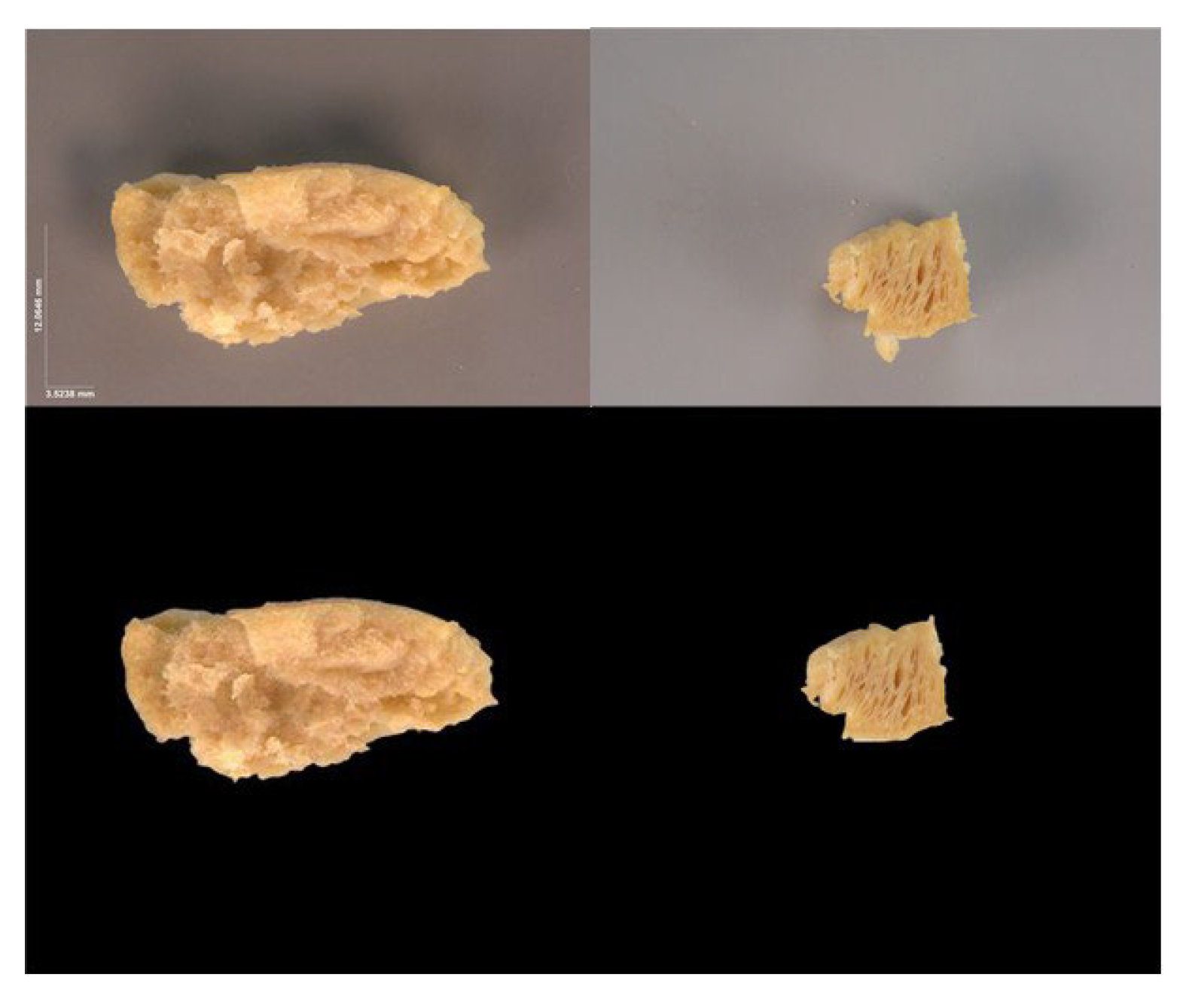
Figure 2.
Eight spatial orientations of a real image.
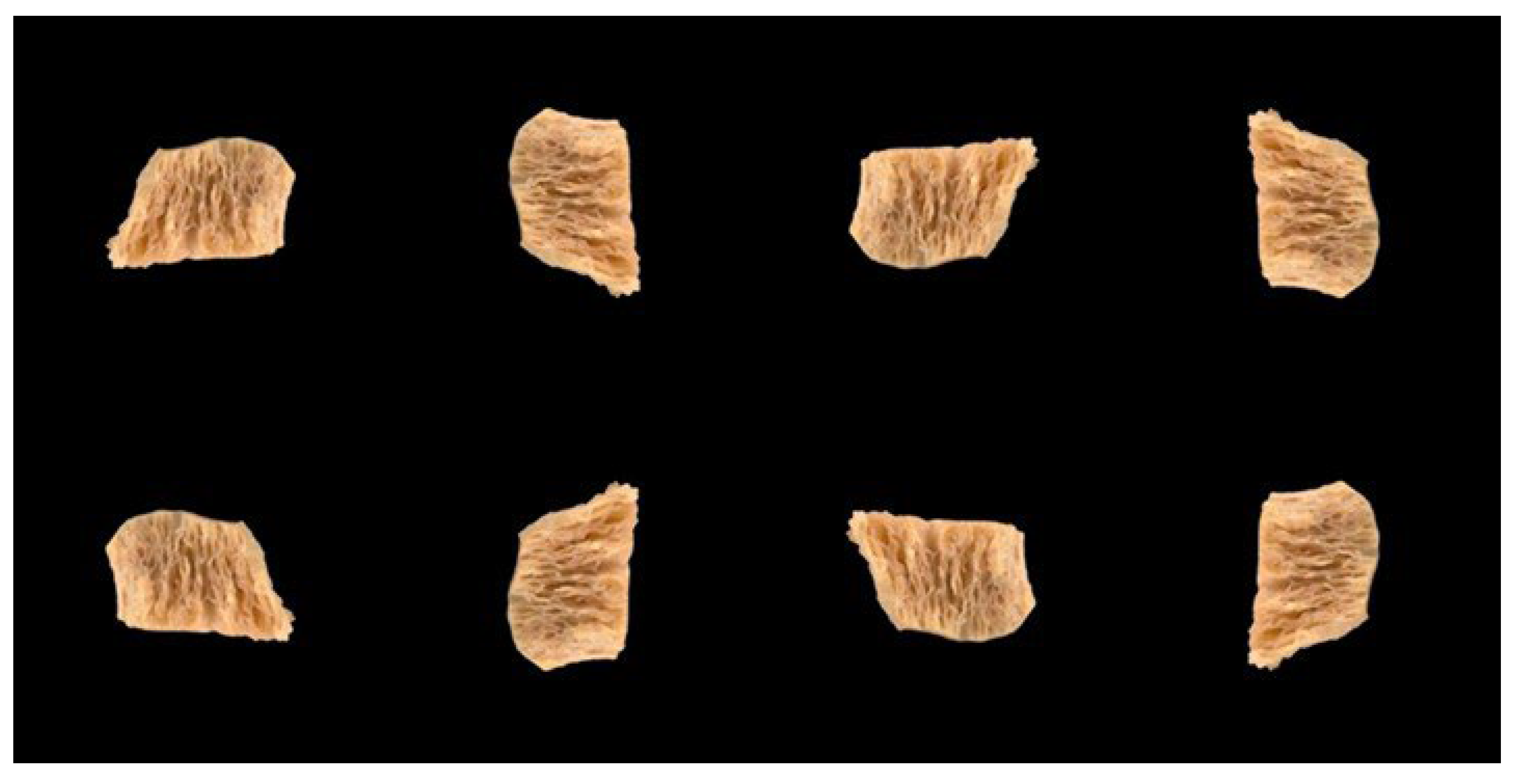
Figure 3.
Synthetic images.
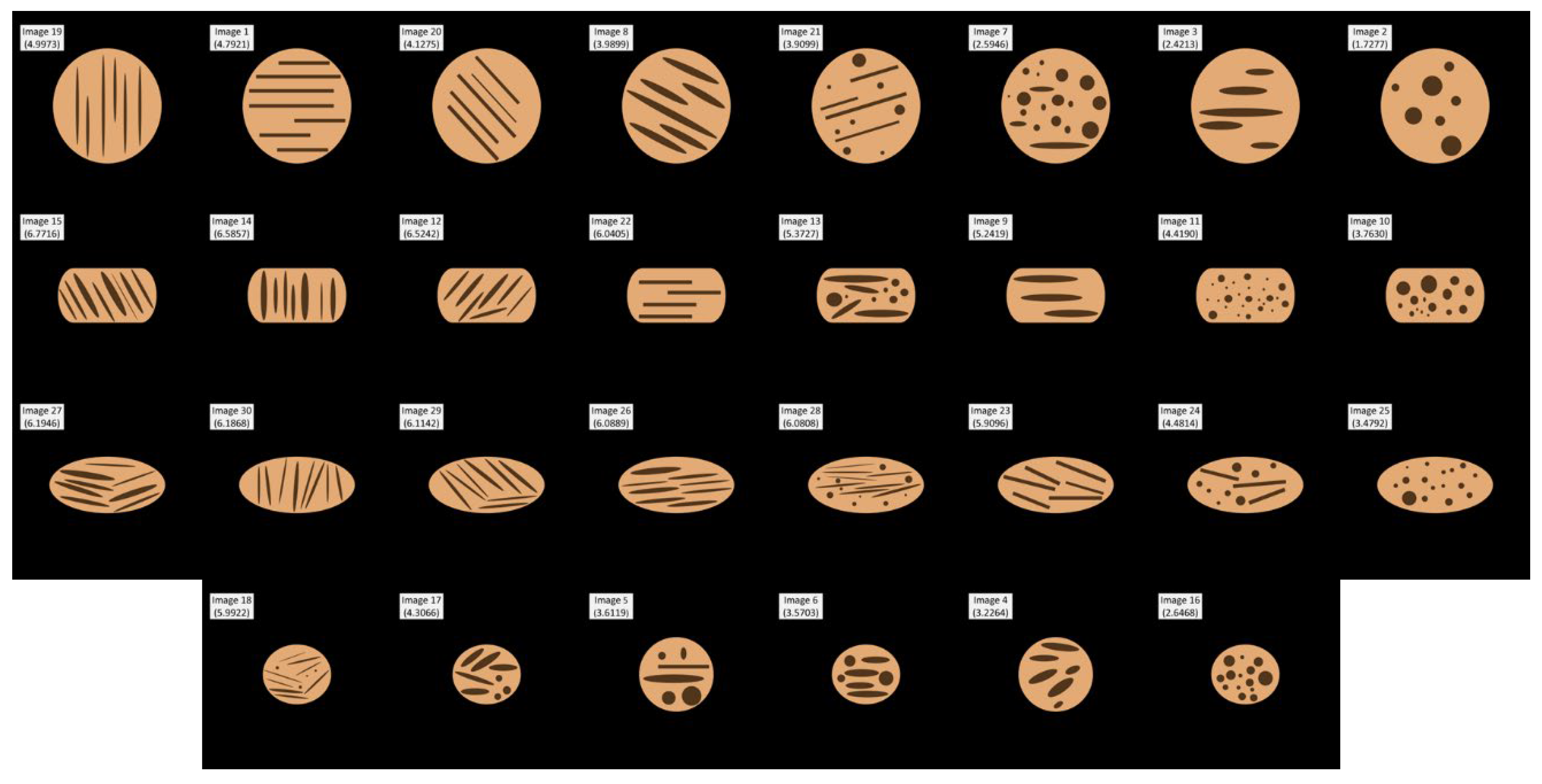
Figure 4.
Proposed DNN architecture.
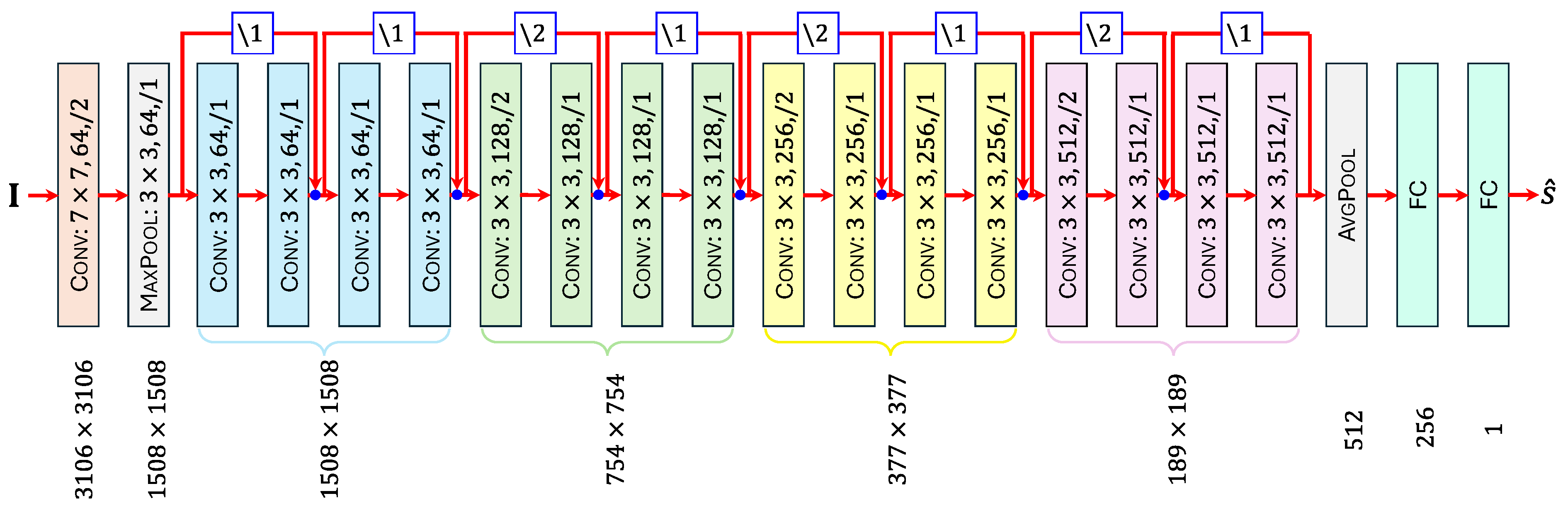
Figure 5.
Learning curves.
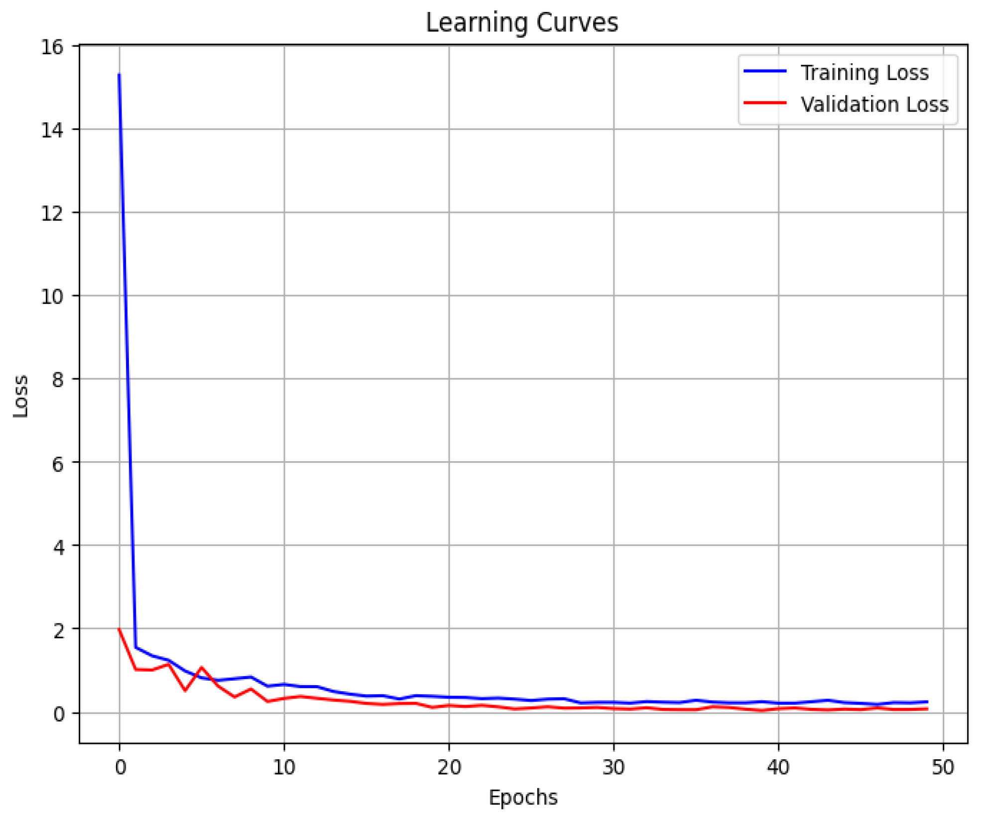
Figure 6.
Scatter plot with combined dataset.
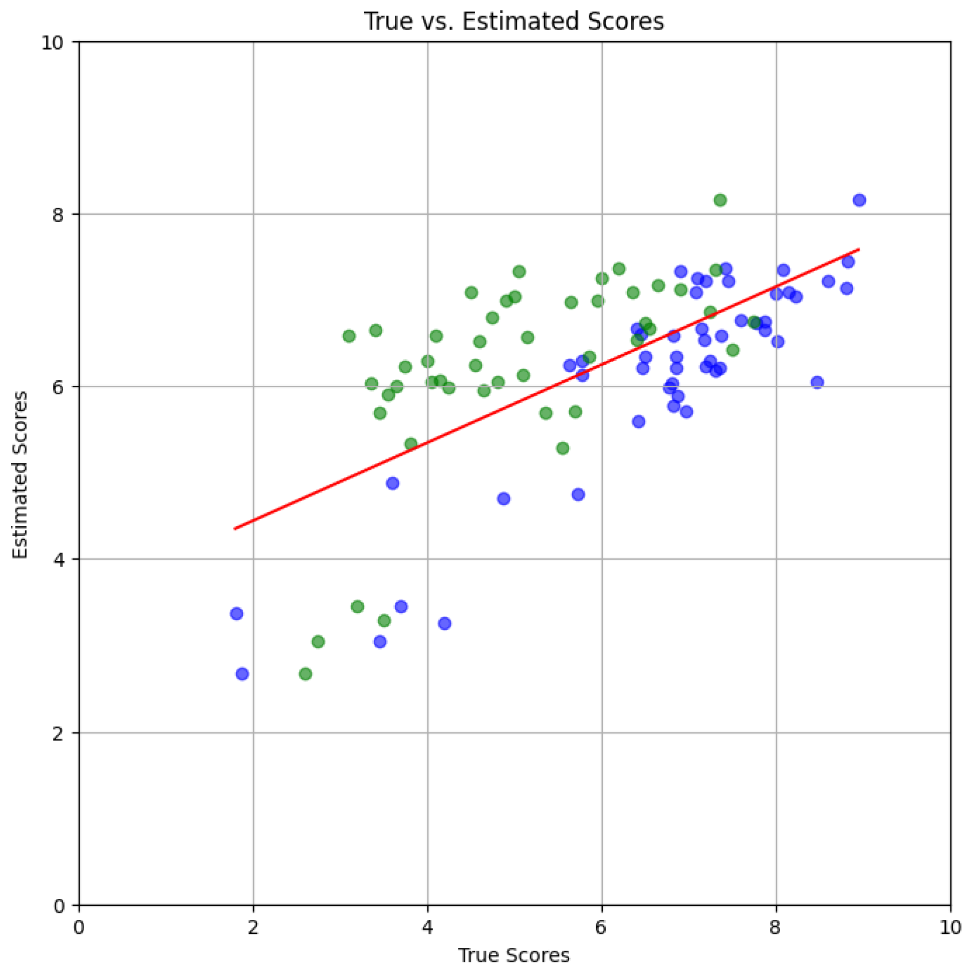
Figure 7.
Scatter plots with individual subjects’ test datasets, (left), (right).
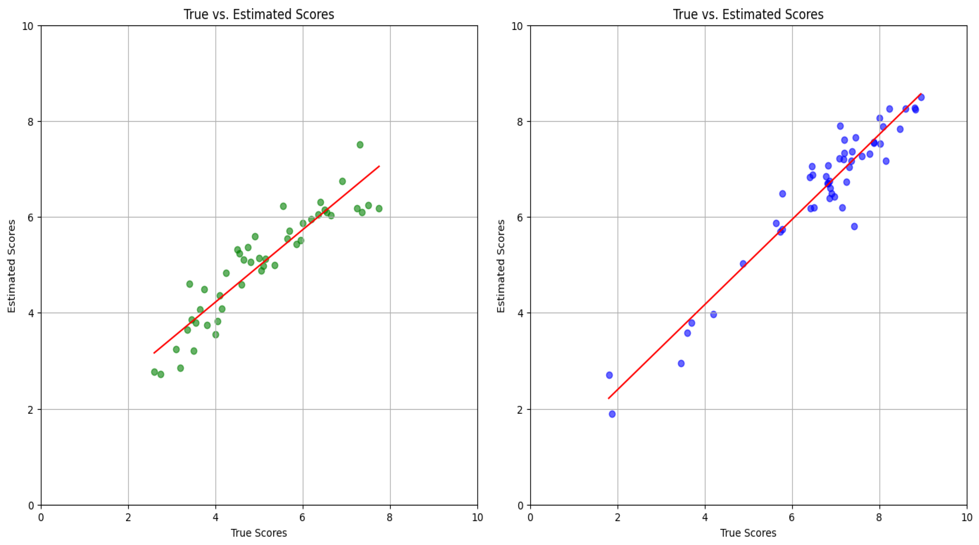

Table 1.
Statistical performance metrics with real images.
| Test Set |
Error Norm | Goodness of Fit | Regression | ||||
|---|---|---|---|---|---|---|---|
| 1.7198 | 1.0471 | 0.4155 | 0.6676 | 1.0038 | 0.45 | 3.54 | |
| 0.3062 | 0.4166 | 0.8387 | 0.9218 | 0.9772 | 0.76 | 1.20 | |
| 0.2229 | 0.3581 | 0.9122 | 0.9594 | 0.9751 | 0.89 | 0.62 | |
Table 2.
Performance with synthetic images.
| No. | Cat. | Estimated Score (32 Orientations) | ||||
|---|---|---|---|---|---|---|
| Avg. | Med. | Min. | Max. | Std. | ||
| 15 | BO | 6.7716 | 6.7152 | 5.8834 | 7.5957 | 0.5084 |
| 14 | BO | 6.5857 | 6.4917 | 6.1085 | 7.2480 | 0.3206 |
| 12 | BO | 6.5242 | 6.3535 | 5.7271 | 7.7302 | 0.5639 |
| 27 | EL | 6.1946 | 6.1781 | 5.5981 | 6.6784 | 0.3570 |
| 30 | EL | 6.1868 | 6.2695 | 5.4897 | 6.8186 | 0.3954 |
| 29 | EL | 6.1142 | 6.1447 | 4.9612 | 6.8343 | 0.4535 |
| 26 | EL | 6.0889 | 6.0014 | 5.5629 | 6.7248 | 0.3779 |
| 28 | EL | 6.0808 | 6.0857 | 5.5080 | 6.8620 | 0.3434 |
| 22 | BO | 6.0405 | 5.9445 | 5.3056 | 6.9674 | 0.4756 |
| 18 | SC | 5.9922 | 5.9873 | 5.5479 | 6.4865 | 0.2265 |
| 23 | EL | 5.9096 | 5.9609 | 5.0529 | 6.6452 | 0.4213 |
| 13 | BO | 5.3727 | 5.3345 | 4.7956 | 6.1312 | 0.3838 |
| 9 | BO | 5.2419 | 5.0952 | 4.2173 | 6.5956 | 0.8068 |
| 19 | LC | 4.9973 | 4.9878 | 4.1453 | 5.8929 | 0.5149 |
| 1 | LC | 4.7921 | 4.7188 | 3.8545 | 6.1682 | 0.6730 |
| 24 | EL | 4.4814 | 4.4687 | 4.1215 | 4.8845 | 0.2288 |
| 11 | BO | 4.4190 | 4.1944 | 3.8615 | 5.5724 | 0.5932 |
| 17 | SC | 4.3066 | 4.2440 | 3.8008 | 4.8826 | 0.3150 |
| 20 | LC | 4.1275 | 4.2039 | 3.3024 | 5.2319 | 0.5109 |
| 8 | LC | 3.9899 | 3.7618 | 2.6536 | 5.4541 | 0.7026 |
| 21 | LC | 3.9099 | 3.9401 | 3.2163 | 4.3710 | 0.3511 |
| 10 | BO | 3.7630 | 3.6224 | 3.3140 | 4.6773 | 0.4312 |
| 5 | SC | 3.6119 | 3.4995 | 3.1894 | 4.4612 | 0.3747 |
| 6 | SC | 3.5703 | 3.6371 | 2.8441 | 4.0011 | 0.3119 |
| 25 | EL | 3.4792 | 3.5238 | 3.1798 | 3.7570 | 0.2044 |
| 4 | SC | 3.2264 | 3.1495 | 2.5932 | 4.1181 | 0.4451 |
| 16 | SC | 2.6468 | 2.6389 | 2.3321 | 2.9631 | 0.1437 |
| 7 | LC | 2.5946 | 2.5982 | 2.3745 | 2.8544 | 0.1170 |
| 3 | LC | 2.4213 | 2.4301 | 1.6123 | 3.2826 | 0.4522 |
| 2 | LC | 1.7277 | 1.7256 | 1.5278 | 1.8731 | 0.0872 |
Disclaimer/Publisher’s Note: The statements, opinions and data contained in all publications are solely those of the individual author(s) and contributor(s) and not of MDPI and/or the editor(s). MDPI and/or the editor(s) disclaim responsibility for any injury to people or property resulting from any ideas, methods, instructions or products referred to in the content. |
© 2025 by the authors. Licensee MDPI, Basel, Switzerland. This article is an open access article distributed under the terms and conditions of the Creative Commons Attribution (CC BY) license.
Copyright: This open access article is published under a Creative Commons CC BY 4.0 license, which permit the free download, distribution, and reuse, provided that the author and preprint are cited in any reuse.


