Submitted:
05 June 2025
Posted:
06 June 2025
You are already at the latest version
Abstract
Traditional deep learning approaches for pork freshness grading require extensive datasets, posing significant challenges in practical applications where sample collection is costly and time-consuming. To reduce the cost of image sample collection, this research aims to develop a few-shot learning method for accurate pork freshness classification with limited data. Utilizing microbial cell concentration as a parameter, a pork freshness grade dataset containing 600 images has been established through physical and chemical testing methods. We propose the BBSNet, a lightweight architecture that integrates BCN, a double attention mechanism (BiFormer), and ShuffleNetV2. The BCN layer enhances feature distinguishability by replacing traditional normalization methods, while the BiFormer module dynamically optimizes attention for fine-grained feature extraction. In the 5-way 80-shot task (where 5 denotes the number of categories and 80 indicates the number of samples in the support set), the accuracies for average accuracy, sensitivity, specificity, and precision are 96.36%, 78.85%, 85.71%, and 96.3%, respectively. These results demonstrate that BBSNet significantly reduces data dependency without compromising accuracy, providing a cost-effective solution for real-time pork quality monitoring. This work presents a novel framework for food freshness assessment under data-scarce conditions, bridging the gap between laboratory-based indicators and industrial applications.
Keywords:
Pork freshness
; Few-shot learning
; Biformer
; Fine-tuning
1. Introduction
With rising living standards, consumers increasingly prioritize meat quality, particularly freshness. Current evaluations of pork freshness predominantly rely on physicochemical methods, such as microbial concentration [1], TVB-N detection[2], and pH measurement[3]. While these methods are accurate, they are also destructive, time-consuming, and unsuitable for rapid online detection[4]. Non-destructive alternatives utilizing spectral imaging and electronic nose technologies have emerged in food quality inspection.[5,6]Hyperspectral imaging (400–1000 nm) combined with least squares support vector machines has enabled effective TVB-N prediction [7], while fluorescence hyperspectral imaging has facilitated the assessment of frozen pork quality through partial least square regression[8]. However, spectral overlap and limited wavelength effectiveness constrain the accuracy of feature extraction. Similarly, electronic nose systems that employ linear discriminant analysis[9] or PCA sensor arrays [10] encounter challenges related to high costs and operational complexity, despite achieving high accuracy [11].
Multimodal approaches that integrate spectral imaging and electronic noses [12,13,14] enhance detection robustness; however, they necessitate dedicated hardware systems that are susceptible to inherent time delays and data synchronization errors. In contrast, computer vision provides rapid, non-destructive alternatives, achieving an accuracy of 92.5% in grading pork color and marbling through support vector machines [15] and estimating intramuscular fat using gradient boosting machines [16]. Furthermore, advanced image processing techniques employing attention-enhanced U-Net models have optimized feature extraction [17]. Nonetheless, deep learning models require large datasets and significant computational resources, while data augmentation techniques are often insufficient for enhancing critical features such as color and texture [18,19,20].
Few-shot learning effectively addresses these limitations by facilitating classification with minimal labeled data[21].Nie et al. (2024)[22] summarized the applications of few-shot learning in the field of intelligent agriculture. By leveraging few-shot learning, the reliance of intelligent agriculture on large datasets is expected to decrease, thereby further enhancing its level of intelligence.R-CNN-based strawberry disease detection achieved an accuracy of 96.67% with only 550 samples [23], while FPGA-ARM embedded systems attained over 95% pest recognition using 350 samples. Nie et al. (2023) [24] enhanced the accuracy and robustness of data-driven artificial neural networks by incorporating expert knowledge, which also reduced their data requirements.These methodologies reduce hardware dependency and improve field applicability, presenting promising solutions for resource-efficient monitoring of pork freshness.
To the best of the authors’ knowledge, no reports have been published regarding the application of few-shot learning techniques to the problem of pork freshness grading. Our contributions include:
i)the development of BBSNet, a lightweight architecture that integrates dynamic attention mechanisms and channel normalization, achieving an accuracy of 96.36% in 5-way 80-shot tasks. This approach addresses the high data dependency characteristic of traditional deep learning methods in pork freshness detection.
ii) The replacement of Batch Normalization in ShuffleNetV2 and Layer Normalization in BiFormer with BCN, which enhances feature stability and discriminability, resulting in a 6.27% improvement in 5-way 5-shot accuracy compared to baseline models.
iii) The performance of BBSNet surpasses that of classic few-shot models (MAML, Prototypical Networks) and CNNs such as AlexNet and ResNet50 under conditions of limited data. BBSNet achieved accuracies of 59.72% (1-shot) and 78.84% (5-shot) in 5-way tasks, demonstrating its adaptability to scenarios with scarce labeled data.
The remainder of the paper is structured as follows: Section 2 details the materials and methods, including dataset acquisition, the few-shot learning method based on BBSNet, model training, and evaluation metrics. Section 3 presents the results and discussions, comparing the performance of various models and analyzing the impacts of the BCN layer, the BiFormer attention mechanism, and the number of support set samples. Section 4 summarizes the findings of the entire paper and provides an outlook on future work.
2. Materials and Methods
2.1 Data Set Acquisition
2.1.1 Pork Freshness Grading Criteria
Total colony count is a critical indicator of meat spoilage, serving as a determinant for the continued consumption of pork. Additionally, positive correlations have been observed among pork color, luster, and other quality attributes [25]. Consequently, microbial colony concentration was utilized as a measure of pork freshness.
Pork samples were obtained from the Jiangsu Taizhou RT-Mart Supermarket. The hind leg meat was cut into pieces measuring approximately 50 mm×80 mm with a thickness of 10 mm, resulting in a total of 500 slices. These slices were then packaged in sterilized self-sealing bags and stored in a refrigerator at 4℃ for durations of 0, 24, 48, 72, and 96 hours. Subsequently, the microbial concentrations of the pork samples were determined in accordance with the GB 47892-2010 standard, “Determination of Microbial Counts in Foods.” The microbial colony concentrations of the pork samples were measured separately, and the average value was calculated to represent the microbial colony concentration parameter for the samples.According to the national standard GB/T 9959.2-2008, which pertains to Split Fresh and Frozen Lean Pork, the total number of bacterial colonies in fresh meat should not exceed 106 CFU/g. After 72 hours of storage at 4℃, the total colony count of the sampled pork reached 1.778279×10⁶ CFU/g, surpassing the standard limit for fresh pork total colony count. Consequently, pork freshness was classified into five grades based on microbial colony concentration parameters, as summarized in Table 1. This grading system closely aligns with the findings of Zhang et al. (2023) [11] and Cheng et al. (2024) [14].
2.1.2. Pork Freshness Dataset
Five pork samples, each representing different freshness grades, were imaged under natural light using a CCD camera. The captured images were subsequently uploaded to a computer via USB for storage. A total of 120 samples were collected for each grade of pork freshness, resulting in an overall dataset of 600 samples. These images were resized to 224×224 pixels for subsequent analysis. The images corresponding to various pork freshness classes are illustrated in Table 2. First-grade and second-grade fresh pork samples exhibited a bright red color with good luster, while third-grade fresh pork samples displayed a dark red hue with an average appearance. In contrast, first-grade and second-grade spoiled pork samples were characterized by a dark red color and poor luster.
A k-way, n-shot task was established, where k denotes the number of categories and n indicates the number of samples in the support set. In this study, pork freshness was categorized into five classes; thus, the research task is defined as a 5-way n-shot task. To validate the model’s performance, n images are randomly selected from each class of the dataset to form the support set.
2.2 Few-Shot Learning Method Based on BBSNet
In few-shot learning, images are mapped to task-specific metric spaces to facilitate similarity-based recognition. Prototypical networks [26] are noted for their simplicity and efficiency. Recent studies have incorporated self-attention mechanisms[27,28,29] to improve feature discrimination. These works demonstrate that attention-driven prototype refinement has the potential to mitigate feature ambiguity in scenarios with limited data.
To address the high computational costs associated with existing attention-enhanced prototypical networks, we propose BBSNet, a lightweight architecture designed for five-class pork freshness classification. Built upon prototypical networks, BBSNet utilizes the ShuffleNetV2 backbone to minimize computational load while integrating the BiFormer module to enhance feature discriminability. Additionally, the BCN normalization method is employed to facilitate stable training with higher learning rates and reduced dependency on initialization.The proposed pipeline involves the following steps:
a)Extracting feature vectors using BBSNet;
b)Computing cosine similarities between query features and the five class prototypes in the support set;
c)Determining the category with the highest similarity through softmax activation. This design effectively balances efficiency and accuracy, as illustrated in Figure 1.
2.2.1. Composition of BBSNet
Metric-based methods typically employ episodic training strategies to train the feature extractor, utilizing either a fixed or parameterized distance metric. This approach places substantial demands on the performance of the feature extraction network. A high-performing feature extraction network is crucial for ensuring the accuracy of metric operations in few-shot learning [30,31].
Figure 2 (a) illustrates the structure of the BBSNet feature extraction network. The input image is processed through a convolutional layer with a 3x3 convolutional kernel and a stride of 2, before entering the first stage after passing through a max pooling layer. This stage comprises the basic unit of ShuffleNetV2 in conjunction with the Patch Merging + BiFormer block module. The second through fourth stages consist of the ShuffleNetV2 downsampling unit alongside the Patch Merging + BiFormer block module. After the original image undergoes processing through four computational stages, it is subsequently passed through a convolutional layer that employs 11 convolutional kernels with a filter size of 1. This is followed by a global average pooling layer, a dropout layer with a dropout rate of 0.4, and a Flatten layer. Consequently, the image features are extracted into a one-dimensional vector. Dropout is utilized for model regularization by randomly deactivating a portion of the neurons, thereby enhancing network sparsity, which is beneficial for feature selection and the prevention of overfitting during training [11]. The Adam algorithm is employed as the model optimizer for the feature extraction network, with the learning rate set to 0.001.
2.2.2. Upgrading of ShuffleNetV2 Module
Although ShuffleNetV2 prioritizes computational efficiency, its effectiveness in fine-grained tasks, such as pork freshness grading, is limited by insufficient feature discrimination. To address this limitation, we enhance the network architecture through two structural innovations.
(a)BCN:
Integrated after each convolutional layer (3×3 depthwise and 1×1), BCN, in conjunction with ReLU, stabilizes feature distributions while preserving discriminative texture and color details.
(b)BiFormer-enhanced dual-branch design:
Basic unit: Features are processed sequentially through depthwise convolution → BCN → patch merging → BiFormer (capturing spatial-channel dependencies) → channel shuffling.
Downsampling unit: Parallel branches reduce spatial resolution by half. The right branch incorporates BiFormer and BCN to facilitate multi-scale feature fusion.
Given the sensitivity of local feature differences, such as color and texture, in images of pork freshness, BCN effectively preserves subtle feature variations across different regions. This is achieved by performing local statistical normalization on image blocks, thereby avoiding the potential blurring of local information that may result from the global normalization approach of BN. The BiFormer module optimizes computational efficiency without compromising feature specificity. Collectively, these modifications strengthen ShuffleNetV2’s ability to discern critical freshness-related patterns in pork images, aligning with the precision requirements of food quality assessment [32].
2.2.3. Accelerating feature fitting with batch channel normalization
Internal variable shifts may occur due to the randomness in parameter initialization and variations in input data [33].BCN integrates the advantages of BN[34] and LN [35] by utilizing the correlations between channels and batch processing.
To address the limitations of traditional BN and LN in capturing both spatial and channel-wise statistics, we adopt BCN proposed by Khaled et al. (2023) [36]. BCN dynamically balances the contributions of batch-wise and channel-wise normalization through a learnable parameter ι, enabling adaptive feature scaling and shifting.
The BCN operation is defined as:
where xi is the input image tensor,Ɩ,γ and β are learnable parameters and ɛ is a small constant used for numerical stability. By adopting BCN method, all channels in convolutional layer shared the same normalization terms μ and σ2, μ1,μ2 and σ12,σ22 denote the mean and variance computed across both batch and channel dimensions.This improved model performance in deep learning networks [37]. In this research, LN layers in BiFormer module and BN layers in ShuffleNet were all replaced with BCN. Here, the learnable parameters Ɩ, γ, and β were all randomly initialized from a normal distribution (with a mean of 0 and standard deviation of 1).
2.2.4 Upgrading of BiFormer module
In recent years, Vision Transformers have made significant advancements in the field of computer vision [38,39]. The existing BiFormer module [40] incorporates a LN layer, which necessitates the computation of a global dimension for each sample, resulting in substantial computational costs. Furthermore, LN demonstrates insensitivity to variations in sequence length, rendering it more appropriate for sequence-based tasks such as natural language processing [35].To mitigate these limitations, this study substitutes the LN layer with a BCN layer, thereby constructing a BCN-BiFormer attention mechanism, as illustrated in Figure 3. The BiFormer module comprises a 3×3 depthwise convolutional layer, a bi-level routing attention layer, a BCN normalization layer, and a dilated multi-layer perceptron (with a dilation ratio of e).The input consists of an H×W×3 three-channel image, which is processed through four stages:
Stage 1: An overlapping patch embedding layer and the BCN-BiFormer module reduce the feature size to H/4×W/4×3.
Stages 2–4: Block merging modules and BCN-BiFormer modules halve the spatial dimensions while doubling the channel count at each stage.
The structure of improved Biformer is illustrated in Figure 3,the DWConv denotes depthwise convolution, the BCN represents batch channel normalization processing, and the MLP refers to a multilayer perceptron.
In Figure 3, the input feature map X, denoted as , is initially subdivided into S×S subregions. Each subregion comprises HW/S2 feature vectors. X is reconstituted as Xr, which belongs to . Subsequently, the feature vectors undergo linear trans formations to generate three matrices, Q, K and V. Attention relations between regions are then obtained by constructing a directed graph to localize the relevant regions of a given region. It is possible to obtain the region level Qr and Kr An expression for the adjacency matrix Arcan be obtained in Eq. (2).
The expression for the routing index matrix Ir can be obtained Eq.(3):
The expression for Kg,Vg can be obtained from Eq. (4):
Lastly, the gathered Kg and Vg undergo attention processing, and an additional term,LCE(V), is incorporated to yield the output tensor O Eq.(5).
In the image classification task, the expansion ratio (e) of the MLP was set to 3, the parameter S was set to 7, and the top-k values in the four-stage BRA were specified as 7, 8, 16, and 49, respectively [40].
2.2.5 Probability Distribution Function Based on Cosine Similarity
The primary differences among images representing various levels of pork freshness were observed in terms of color and luster. As detailed in Section 2.1, experimental verification indicated that with prolonged storage time, the color of the pork deepened while its luster diminished. In digital images, despite variations in luster, the directions of feature vectors for the same image remained largely consistent, which made it challenging to distinguish subtle differences. However, utilizing cosine similarity proved effective in differentiating the directions of feature vectors, thereby enhancing the model’s performance.
To accurately assess the similarity of image features, this research employed cosine similarity [41] as a metric for evaluating image similarity. As outlined in Section 2.1, it was posited that the support set comprised five types of images, corresponding to the five classes of the pork freshness dataset, with each class containing n samples. Consequently, a 5-way, n-shot task was executed. The feature vectors of the support set images were extracted using a convolutional neural network, resulting in n feature vectors for each class.
The n feature vectors were averaged and subsequently normalized to yield five one-dimensional feature vectors:.Figure 4 illustrates the calculation process. The vector q was derived following the feature extraction and normalization of each image in the query set using the same convolutional neural network.
After the normalization processing of query and support set image vectors, cosine similarity values among the vector q and were compared. As presented in Figure 5, cosine similarity value was denoted as . Here, θ is the angle between the two vectors being compared, and the smaller the value of θ, the greater the similarity between the two vectors. Cosine similarity was expressed as:
where is the mean vector of the nth support set, is the 2-norm of the vector , and is the 2-norm of the vector q.
Softmax classifier was applied to predict the similarity between support and query sets.
where M is the mean vectors of the samples of the five pork freshness categories in the support set, which was defined as:
and q is the feature vector of query set. Then, the probability distribution p of query set samples was defined as:
2.3 Fine-Tuning Strategy
This study presents a cosine similarity-based fine-tuning framework that incorporates an adaptive softmax classifier to enhance few-shot recognition. After pre-training the BBSNet feature extractor on support set samples, both support and query images are encoded into one-dimensional feature vectors. The cosine similarities between these vectors are processed through a softmax classifier, whose parameters are optimized using support set data to align the weight vectors with intrinsic feature similarity patterns. To maintain computational efficiency, the pre-trained BBSNet parameters remain frozen during the fine-tuning process. The optimization employs a two-stage strategy for each epoch:
(a)Cross-entropy minimization on support set samples refines the classification boundaries; (b) Entropy regularization applied to query set features mitigates overfitting and enhances discriminability.
This dual mechanism synergistically improves model generalizability, resulting in significant accuracy gains in few-shot tasks while preserving computational efficiency.
2.3.1. Updating Cross-Entropy Loss Function
To distinguish between model training samples and fine-tuning samples, during fine-tuning process, the samples and labels in support set were denoted as . Here, is the feature vector extracted through BBSNet and pj is the predicted label of the model, defined as:
As described in Section 2.2, to accelerate fine-tuning convergence speed, the value of W was initialized to M and b was set as a zero column vector. Here, M is the mean of feature vectors in support set.
During fine-tuning process, support set samples were applied as training samples and cross-entropy loss function was used to update the values of W and b. Cross-entropy loss function was calculated using Eq. (13), where yj is true label and pj is predicted label.
2.3.2 Updating Entropy Regularization Function
During the updating process of cross-entropy loss function, due to the small number of training samples, the model was prone to overfitting. In this research, entropy regularization was added to cross-entropy loss function to prevent overfitting.
An image in query set was denoted as A. The feature vector extracted by BBSnet was denoted as . Probability was calculated using softmax activation function as a probability distribution . Assuming that there were m samples in query set, the entropy regularization term of m samples was denoted as H(p)
where i is the number of samples in query set. H(p) measured the amount of probability distribution p information. Substituting Eq.(14) into Eq.(13), the loss function in fine-tuning process was obtained as:
By incorporating the entropy regularization term of the query set into the loss function, the optimizer subtracts this regularization term in each epoch. When the regularization term is large, a significant value is deducted in each epoch, thereby accelerating the convergence speed of the loss function.
2.4 Model Training
2.4.1 Pre-training setting
The model was compiled in Windows environment on computer with I7-8700 CPU, 8G of memory, and NVIDIA GTX1060 6G graphics card. All the code was implemented using Keras framework based on TensorFlow 2.0 version.
2.4.2 Pre-training setting
The mini-ImageNet dataset is widely utilized in the field of few-shot image recognition. It comprises 100 categories, featuring images of various objects such as fish and birds. Few-shot learning aims to classify unknown images by leveraging the characteristics of known images. Consequently, in accordance with classification principles, mini-ImageNet has been partitioned into a training set, a test set, and a validation set, as detailed in Table 3.
The few-shot feature extraction network was pre-trained using a transfer learning method [15] to obtain the initial model weights. To accomplish the classification task involving 100 categories of images from the mini-ImageNet dataset, the flatten layer of the convolutional neural network model was removed during pre-training. The fully connected layer utilized 100 neurons for output. The Adam optimizer was employed during the backpropagation process, with the cross-entropy loss function applied, and the softmax function used for classification. The learning rate was set to 0.0001. The initial weights of BBSNet were obtained after completing 40 epochs.
2.5 Model Evaluation Metrics
Model evaluation parameters included true positives (TP), true negatives (TN), false positives (FP), and false negatives (FN) [42]. In this research, accuracy (Acc), sensitivity (Sen), specificity (Spe), and precision (Pre) were adopted as model evaluation metrics. Specific calculation equations were expressed as follows:
where TP is the number of positive samples correctly classified as positive, TN is the number of negative samples correctly classified as negative, FP is the number of negative samples incorrectly classified as positive, FN is the number of positive samples incorrectly classified as negative, l is the total number of sample categories, and i is evaluation metric for each category.
3 Results and Discussions
3.1 Performance Comparison with Classic Algorithms
3.1.1 Comparison with Classic Few-Shot Models
To evaluate the performance of the few-shot model developed in this research, a comparative experiment was conducted between our model and several classic few-shot models, including MAML [43], Matching Networks [44], Prototypical Networks [26], and Relation Networks [45]. All models underwent pre-training using the Mini-ImageNet dataset, and their performance was assessed on two tasks: 5-way 1-shot and 5-way 5-shot learning. The results are summarized in Table 4.
The pre-trained features of classical models and small sample models on general datasets, such as mini-ImageNet, often struggle to capture the unique color and texture variations of food, as exemplified by the color attenuation resulting from the oxidation of pork fat. In this study, we employ the Biformer module to fuse local details, such as muscle fiber texture, with global image features, thereby enhancing sensitivity to key indicators of food spoilage. The BCN layer mitigates the distribution shift between the pre-trained domain (mini-ImageNet) and the target domain (pork images), thereby improving the stability of feature representation. Additionally, the cosine similarity comparison method optimizes the alignment of feature directions, enhancing the aggregation capability of similar samples. Under extremely low sample conditions (1-shot), the model presented in this study achieves an accuracy rate of 59.72%, significantly outperforming other models. This result demonstrates that the model effectively addresses the overfitting issue through pre-training initialization and the injection of prior knowledge, such as the physicochemical principles of food spoilage. Furthermore, the accuracy of 78.84% in the 5-shot task indicates that the model can rapidly capture essential task characteristics with a limited number of samples, thereby reducing reliance on labeled data. Consequently, this research achieves superior performance in the task of pork freshness recognition.
3.1.2 Comparison against classical universality algorithms
Several classic deep learning network models, including AlexNet [46], VGG16 [47], GoogLeNet [48], and ResNet50 [49], were selected to predict pork freshness. The results obtained from these models were compared with those from the few-shot learning model developed in this research. During the training process of the few-shot model, a 5-way, 80-shot method was adopted following the preset pre-training; specifically, for a 5-class classification task, 80 images were provided for each category as training samples. All models utilized 400 images as training samples. The test results are presented in Table 5.
Table 5 illustrates that the average accuracy of the few-shot model developed in this research is 96.36%, significantly surpassing that of traditional network models. This finding indicates that our model achieved the highest classification accuracy for both true positive and true negative samples, reflecting superior classification performance. Furthermore, the model’s average specificity and average precision were recorded at 85.71% and 96.35%, respectively, both of which represent the highest values among all evaluated models. In terms of model sensitivity, the average sensitivity of the proposed model was 78.85%, ranking second only to the ResNet50 model, suggesting that our model also demonstrated relatively high recognition accuracy for true positive samples.
AlexNet, VGG16, and GoogLeNet, three classical models, are constrained by their shallow architectures and limited parameter capacities, resulting in significantly inferior performance metrics. This observation highlights the severe overfitting issue present in these classic models when trained on small sample datasets. Although ResNet50 mitigates the problem of deep network degradation through the use of residual structures, its reliance on large-scale data for training hampers the effective optimization of numerous parameters in scenarios with limited samples, leading to suboptimal performance metrics. This research model is based on the lightweight backbone network of ShuffleNetV2, which boasts a parameter count of approximately 2.3 million (representing 9% of ResNet50) and achieves an exceptionally low computational cost, with a training time of only 59 minutes. Furthermore, BCN normalization addresses gradient fluctuations during small-batch training by decoupling batch statistics from channel statistics. Traditional BN suffers a significant decline in performance when the batch size is less than 16. Classical models depend on fully connected layers for decision-making in classification tasks and necessitate large-scale datasets to effectively learn classification boundaries. In this research, we employ cosine similarity to directly compare the directions of feature vectors, thereby reducing parameter dependence and enhancing applicability in scenarios with limited sample sizes. In summary, when the number of samples is constrained, small sample methods demonstrate significant advantages across all dimensions compared to classical neural network models that require extensive datasets for training.
3.2 Batch Channel Normalization Impacts
The purpose of normalization is to enhance training efficiency, reduce the risk of overfitting, and improve network stability and generalization capabilities. In this study, the BCN layer was utilized to replace the BN layer in the ShuffleNetV2 model, while the LN layer in the BiFormer module was substituted with the BCN layer to optimize model performance. To evaluate the optimization effect of the BCN layer in the feature extraction network, we compared the accuracies of the model using BCN, BN, and LN layers across two tasks: 5-way 1-shot and 5-way 5-shot. In the 5-way 1-shot task, only one sample was drawn from each category, resulting in a total of five samples for model training. Conversely, in the 5-way 5-shot task, five samples were drawn from each category, leading to a total of 25 samples for model training. Subsequently, 100 samples with varying freshness levels were randomly selected as the test set to assess the prediction accuracy of the model after few-shot training. The results are summarized in Table 6.
As presented in Table 6, the integration of BCN layers resulted in an improvement of 4.21% in 5-way 1-shot accuracy and 6.27% in 5-way 5-shot accuracy compared to the baseline model. This enhancement can be attributed to BCN’s dual normalization framework, which combines the advantages of BN and LN. Specifically, BCN stabilizes the training process by normalizing per-channel features while leveraging batch statistics, including mean and variance. Compared to BN, BCN exhibits superior robustness in small-batch scenarios due to its channel-wise normalization, which mitigates noise interference caused by inaccurate batch statistics (Li et al., 2019). In few-shot learning tasks characterized by limited data and imbalanced class distributions, the BCN layer effectively mitigates overfitting risks by dampening fluctuations in feature distributions while enhancing the model’s discriminative ability for few-shot features.
In ShuffleNetV2, substituting BN with BCN resulted in improvements of 1.33% and 1.95% in 5-way 1-shot and 5-shot accuracy, respectively. This enhancement is attributed to BCN’s ability to reinforce inter-channel correlations. Traditional BN relies on spatial statistics in image tasks, which are susceptible to noise contamination under few-shot conditions [34]. In contrast, BCN enforces uniform feature scaling across channels through channel-wise normalization, thereby improving feature consistency and discriminability. Notably, BCN maintains a computational complexity comparable to that of BN without incurring additional memory overhead, rendering it suitable for lightweight model optimization.In the BiFormer module, replacing LN with BCN resulted in more significant improvements of 3.26% (1-shot) and 5.06% (5-shot), surpassing the gains observed in ShuffleNetV2. This discrepancy arises from the distinct operational principles of LN and BCN. LN, originally designed for NLP, normalizes sequence dimensions per sample to handle long-range dependencies [35]. However, in image processing tasks, the spatial structures (e.g., edges, textures) exhibit local correlations, and LN’s sample-level normalization may disrupt inter-channel semantic associations [50]. BCN addresses this limitation through global channel-wise normalization, preserving local spatial consistency while promoting inter-channel collaboration, which aligns better with hierarchical visual feature learning [51].
3.3 BiFormer Attention Mechanism impacts
The BiFormer attention mechanism enhances image processing by allowing the model to concentrate on the most relevant regions and features. To assess the impact of introducing the BiFormer attention module on the model, the BiFormer module was integrated into the ShuffleNetV2 network, along with the incorporation of patch merging and BiFormer modules into the backbone network. The results obtained after substituting the BN layer in ShuffleNet and the LN layer in the BiFormer module with the BCN layer are summarized in Table 7. All comparison results presented in Table 7 were computed using the fine-tuning method.
Using ShuffleNetV2 as the baseline, the gradual integration of BCN-BiFormer yields significant performance improvements, as shown in Table 7. Incorporating BCN-BiFormer into the backbone alone enhances 1-shot accuracy by 3.29%, increasing it to 55.73%, while 5-shot accuracy sees a modest increase of 0.1%, reaching 69.62%. This underscores the effectiveness of BCN-BiFormer in extracting discriminative features from limited samples. Further deployment of BCN-BiFormer in the backbone backend leads to additional improvements, raising 1-shot and 5-shot accuracy to 57.91% (+5.47% compared to the baseline) and 71.61% (+2.09% compared to the baseline), respectively, thereby validating its role in enhancing high-level feature fusion.Notably, joint integration of BCN-BiFormer in both the backbone and backend results in substantial gains: 1-shot accuracy reaches 59.72% (+7.28% compared to the baseline), while 5-shot accuracy surges to 78.84% (+9.32% compared to the baseline), exceeding the cumulative effects of single-position enhancements. This synergy highlights BiFormer’s dual roles: enhancing feature discriminability in the backbone for few-shot generalization and refining decision boundaries through weighted feature fusion in the backend. In the 5-shot scenario, the increased number of support samples further amplifies BiFormer’s feature refinement, leading to significant improvements in inter-class discrimination.These results demonstrate that BCN-BiFormer systematically enhances few-shot classification performance through multi-layer feature enhancement, providing empirical evidence for the efficacy of leveraging attention mechanisms to boost model representational power.
In contrast to traditional channel attention[52] and spatial attention [53], BiFormer achieves fine-grained feature selection through joint optimization of channel-spatial sparse weights. During few-shot learning, where models must rapidly adapt to novel categories, dynamic attention mechanisms enhance class-discriminative features by dynamically focusing on category-specific regions while suppressing background noise interference.The integration of BiFormer with Patch Merging further strengthens multi-scale feature interactions, thereby improving generalization capabilities in few-shot scenarios. The core advantage of BiFormer lies in the synergy between dynamic sparsity and cross-level feature fusion, enabling efficient capture of discriminative features under limited data. Unlike similar attention mechanisms such as DynamicViT[54] and Deformable Attention[39], BiFormer’s hash routing and lightweight architecture are uniquely suited to the computational constraints and rapid adaptation requirements of few-shot tasks.
3.4. Number of Support Set Samples Impacts
To reduce training time and computational load, the pre-training of few-shot models is typically conducted solely during the extraction of image feature vectors. The number of support set samples refers to the quantity of samples from a single category within each task. This quantity provides prior knowledge to the model, enabling it to perform classification tasks by leveraging this information. Consequently, the number of support set samples significantly influences model performance. During the fine-tuning process, support set samples are utilized to train and optimize the model; thus, the optimization effectiveness of fine-tuning is inevitably impacted by the number of support set samples. To evaluate the effect of the number of support set samples on model performance, the support set was configured with sample sizes of 1, 5, 10, 20, 40, 80, 100, and 120 to assess model accuracy. The results are summarized in Table 8.
In pork freshness recognition, Table 8 illustrates the relationship between support set size and model accuracy in BBSNet. Fine-tuning consistently enhances accuracy across all support set sizes. For instance, it increases accuracy by 3.08% at the 1-shot setting and by 9.1% at the 80-shot setting, corroborating the findings of Chen et al. (2021) [41] regarding the task-specific adaptation of pre-trained features for domain-specific attributes such as pork oxidation. When the support set reaches 80 samples, accuracy plateaus at 96.36%, and increasing the sample size to 120 does not yield any improvement. This suggests that 80 samples effectively encompass the primary features of pork spoilage (such as color and texture), as described by Kyung et al. (2024) [55]. Additional samples likely introduce redundant data, consistent with the “core set” theory in few-shot learning [56], which posits that marginal gains diminish once critical diversity is achieved. The architecture of BBSNet effectively addresses these challenges. The Biformer module integrates local texture such as muscle fiber disintegration and global color to maximize information extraction from limited samples, accounting for the observed 3% accuracy gain for each doubling of samples below 80.
Recent studies corroborate these findings. Yuan et al. (2020) [57] demonstrated that meta-learning models can achieve up to 90% of maximum accuracy with only 50 to 100 samples in fine-grained tasks, which is comparable to BBSNet’s saturation point at 80 samples. Zhao et al. (2024) [58] indicated that the diversity of the support set, rather than its size, is the key factor driving few-shot performance. This principle is effectively leveraged by BBSNet, which emphasizes physicochemical features. For practical applications, the threshold of 80 samples provides an optimal balance between cost and performance.
3.5. Number of Query Set Samples Impacts
The ratio of the Support Set to the Query Set wields a significant influence over the model’s training efficiency and generalization capabilities [59]. In the domain of few - shot learning, the support set functions as the limited labeled data that enables the model to rapidly adapt to novel tasks. Conversely, the query set represents the data used to assess the model’s performance. A query set that is relatively small compared to the support set may result in overfitting, as the model may lack a sufficient variety of samples to generalize effectively beyond the support set instances [60]. Conversely, a larger query set offers more opportunities for the model to discern underlying patterns and enhance its generalization, yet it may also augment the computational load and training time[61].
To investigate the impact of query set size on the performance of the few-shot learning model for pork freshness recognition, we fixed the support set size at 5-way and 5-shot, while varying the number of samples in the query set to 5, 10, 15, 20, 25, 30, and 35. We subsequently measured the model’s classification accuracy and training time. As illustrated in Table 9, the classification accuracy increased steadily from 56.64% to 78.84% as the query set size expanded from 5 to 25. This trend suggests that a larger query set facilitates improved parameter tuning, thereby enhancing the model’s capability to recognize features indicative of pork freshness.
Notably, when the query set size was further increased to 30 and 35, the accuracy decreased slightly to 77.21% and 77.19%, respectively. This decline may be attributed to the model overfitting to the specific characteristics of the larger query set rather than learning the underlying general patterns of pork freshness. Similar observations were reported by Triantafillou et al. (2020) [62], who suggested that an excessively large query set can introduce noise and complexity, thereby degrading the model’s generalization performance. In terms of training time, a positive correlation was observed between the query set size and the training duration, as expected. More samples in the query set required additional computational resources for processing, which led to longer training times. This trade-off between accuracy and training efficiency emphasizes the importance of identifying an optimal query set size for practical applications.
In terms of training time, as anticipated, the increase in the number of query set samples results in a gradual lengthening of the model’s training duration. This phenomenon occurs because a greater number of samples requires additional computational resources and time for the model to process and update its parameters. The trade-off between accuracy and training time highlights the importance of carefully selecting an appropriate query set size. Compared to previous research [63], which also investigated the impact of query set size on few-shot learning models, our findings consistently demonstrate the existence of an optimal query set size that balances the model’s generalization ability with computational efficiency. This discovery not only enhances our understanding of the role of query set samples in few-shot learning but also provides practical guidance for future research and applications in related tasks, such as food quality assessment.
3.6. Validation of Model Generalization on Large-Scale Unknown Samples
To validate the model’s ability to recognize unknown samples, this study conducted additional experiments using the Food-101 dataset[64], a widely recognized benchmark for food recognition tasks. The dataset consists of 101 food categories, each containing 1,000 images, resulting in a total of 101,000 images. This large-scale evaluation ensures the statistical significance of the results and verifies the model’s robustness under data-scarce conditions. Given the ample number of samples, this study selected a 5-way 80-shot task to assess the model’s performance, with five randomly chosen categories in each training round. In the support set, 80 samples were selected from each category, yielding a total of 400 images. As discussed in Section 3.5, the number of query set samples is set to five times that of the support set, totaling 2,000 samples, with stratified sampling employed to ensure equal representation across all samples [65].The model pre-training method, detailed in Section 2.2.4, utilizes fine-tuning to enhance model performance. The experimental results are presented in Table 10.
The model demonstrated superior accuracy on the pork freshness dataset, achieving 96.36% compared to 92.4% in Food101. This indicates an enhanced discriminative capability in freshness assessment. The performance disparity may be attributed to two potential factors.
The model demonstrated superior accuracy on the pork freshness dataset, achieving 96.36% compared to 92.4% in Food101. This indicates an enhanced discriminative capability in freshness assessment. The performance disparity may be attributed to two potential factors:
(a)The intrinsic biological indicators of pork deterioration, such as changes in color gradients, variations in surface texture, and profiles of volatile compounds, which provide more distinctive feature representations than the subtle inter-class differences present in the 101-category fine-grained food classification task of Food101 [64];
(b)The model architecture may inherently prioritize domain-specific feature extraction mechanisms relevant to freshness detection.
Furthermore, the sensitivity disparity (89.6% vs. 78.85%) reveals fundamental characteristics of the task. While the model effectively identifies true positive samples in Food101’s multi-class scenario, its reduced sensitivity in assessing pork freshness likely reflects ambiguities associated with transitional states—samples exhibiting partial biochemical decay characteristics that complicate the clear categorization of fresh versus spoiled. This observation aligns with the specificity results (94.1% vs. 85.71%), where the lower specificity for pork freshness indicates an increase in false positives during spoiled meat detection, possibly due to overlapping spectral features between borderline fresh samples and early-stage spoiled specimens.The precision metrics further underscore the domain-dependent behavior of the model. The significantly higher precision in predicting pork freshness (96.35% compared to 91.8%) indicates that when the model classifies a sample as ‘fresh’, it exhibits a 96.35% confidence level in its accurate identification. This precision-sensitivity trade-off suggests that the model employs a conservative classification strategy for freshness detection, prioritizing the reliability of positive predictions, albeit at the potential cost of overlooking marginal cases. Such behavior may be biologically justified, considering food safety requirements, where false negatives (misclassifying spoiled meat as fresh) pose greater risks than false positives.
To further interpret the model’s generalization performance on unseen datasets, we analyzed the feature maps generated by convolutional layers to visualize the discriminative patterns that drive predictions [47].The feature maps of different datasets are shown in Figure 6 and Figure 7.
For the Food101 dataset, feature activations predominantly concentrate on surface details, such as the texture of bread and the fibers of beef, as well as the overall color distribution, which aligns with the requirements of fine-grained classification. In the context of pork freshness detection, the model emphasizes local biological characteristics: fresh samples exhibit high-intensity activation of uniform red muscle tissue, while spoiled samples activate dim discolored areas and demonstrate abnormal textures. For ambiguous transition samples, the feature maps present a mixed activation pattern of fresh and spoiled regions, resulting in reduced sensitivity (78.85%). This reflects the model’s decision-making difficulties when confronted with contradictory features, such as partially discolored areas that still possess a normal texture. The high precision (96.35%) arises from the strong consensus activation of clear fresh features, characterized by uniform red coloration and intact fibers[66], indicating that the model adopts a conservative strategy—classifying an item as ‘fresh’ only when the features are highly consistent, thereby prioritizing food safety.
4. Conclusions
This study demonstrates that BBSNet—a novel few-shot framework integrating pre-trained weight optimization and BiFormer-BCN hybrid feature extraction—achieves state-of-the-art performance in pork freshness detection under extreme data scarcity, attaining an accuracy of 96.36% at 5-way 80-shot. By efficiently capturing discriminative features, such as color and texture decay, and optimizing task configuration with a support set of 80 and a query/support ratio of 5:1, BBSNet significantly outperforms existing meta-learning benchmarks, including MAML and Relation Networks, as well as deep CNN architectures like ResNet50 and VGG16. Moreover, it prioritizes high-precision prediction of the fresh class, achieving an accuracy of 96.35%, thereby mitigating the risks of false negatives in food safety. Future research should focus on enhancing multimodal generalization and facilitating edge deployment, aiming to address the current challenges posed by imaging diversity and computational complexity in industrial applications.
Author Contributions
Conceptualization, Methodology, Software, Investigation, Formal Analysis, Writing Original Draft,C.L.;Writing Review and Editing;J.H.;Data Curation, Writing - Original Draft;,J.Z.;Conceptualization, Funding Acquisition, Resources, Supervision, Writing Review and Editing;K.C.
Funding
This work was supported by The National Key R&D Program during the 14th Five-Year Plan period (2022YFD2100500); Taizhou Science and Technology Support Program (Social Development) Project (2023-32) and Outstanding Young Backbone Teachers of the “Qinglan Project” in Jiangsu Province (Letter of Jiangsu Teachers [2022] No. 51)
Data Availability Statement
Relevant data supporting the findings of this study are available from the corresponding author upon reasonable request.
Conflicts of Interest
All authors declare no conflicts of interest
Abbreviations
The following abbreviations are used in this manuscript:
| BBSNet | BCN-BiFormer-ShuffleNetV2 |
| BCN | Batch Channel Normalization |
| TVB-N | Total Volatile Basic Nitrogen |
| FPGE -ARM | Field-Programmable Gate Array-Advanced RISC Machines |
| BBSNet | BCN-BiFormer-ShuffleNetV2 |
| BCN | Batch Channel Normalization |
| TVB-N | Total Volatile Basic Nitrogen |
| FPGE -ARM | Field-Programmable Gate Array-Advanced RISC Machines |
| MAML | Model-Agnostic Meta-Learning |
| CNNs | Convolutional Neural Networks |
| BN | Batch Normalization |
| LN | Layer Normalization |
References
- Yang, Z.; Chen, Q.; Wei, L. (2024). Active and smart biomass film with curcumin pickering emulsion stabilized by chitosan adsorbed laurate esterified starch for meat freshness monitoring. International Journal of Biological Macromolecules, 275. [CrossRef]
- Zhang, F.; Kang, T.; Sun, J.; Wang, J.; Zhao, W.; Gao, S.; et al. (2022). Improving tvbn prediction in pork using portable spectroscopy with just in time learning model updating method. Meat Science, 188, 108801. [CrossRef]
- Cheng, M.; Yan, X.; Cui, Y.; Han, M.; Wang, X.; Wang, J.; et al. (2022). An ecofriendly film of phresponsive indicators for smart packaging. Journal of Food Engineering, 321, 110943. [CrossRef]
- Lee, S.; Norman, J.M.; Gunasekaran, S.; Laack, R.L.J.M.V.; Kim, B.C.; Kauffman, R.G. (2000). Use of electrical conductivity to predict water holding capacity in post rigor pork sciencedirect. Meat Science, 55(4),385389. [CrossRef]
- Nie, J.; Wu, K.; Li, Y.; Li, J.; Hou, B. (2024). Advances in hyperspectral remote sensing for precision fertilization decision making: a comprehensive overview. Turkish Journal of Agriculture and Forestry, 48 (6), 10841104. [CrossRef]
- Zhou, L.; Wang, X.; Zhang, C.; Zhao, N.; Taha, M.F.; He, Y.; Qiu, Z. (2022).Powdery Food Identification Using NIR Spectroscopy and Extensible Deep Learning Model.Food and Bioprocess Technology,15(10),23542362. [CrossRef]
- Guo, T.; Huang, M.; Zhu, Q.; Guo, Y.; Qin, J. (2017). Hyperspectral image based multi feature integration for tvbn measurement in pork. Journal of Food Engineering, 218(feb.), 6168. [CrossRef]
- Zhuang, Q.; Peng, Y.; Yang, D.; Wang, Y.; Zhao, R.; Chao, K.; et al. (2022). Detection of frozen pork freshness by fluorescence hyperspectral image. Journal of food engineering(Mar.), 316. [CrossRef]
- Musatov, V.Y.; Sysoev, V.V.; Sommer, M.; Kiselev, I. (2010). Assessment of meat freshness with metal oxide sensor microarray electronic nose: a practical approach. Sensors & Actuators B Chemical, 144(1), 99103. [CrossRef]
- Tian, X.Y.; Cai, Q.; Zhang, Y.M. (2012). Rapid classification of hairtail fish and pork freshness using an electronic nose based on the pca method. Sensors, 12(12), 260278.
- Zhang, J.; Wu, J.; Wei, W.; Wang, F.; Jiao, T.; Li, H.; Chen, Q. (2023).Olfactory imaging technology and detection platform for detecting pork meat freshness based on IoT.Computers and Electronics in Agriculture,215,Article 108384. [CrossRef]
- Huang, L.; Zhao, J.; Chen, Q.; Zhang, Y. (2014). Nondestructive measurement of total volatile basic nitrogen (tvbn) in pork meat by integrating near infrared spectroscopy, computer vision and electronic nose techniques. Food Chemistry, 145(feb.15), 228236. [CrossRef]
- Liu, C.; Chu, Z.; Weng, S.; Zhu, G.; Han, K.; Zhang, Z.; Huang, L.; Zhu, Z.; Zheng, S. (2022). Fusion of electronic nose and hyperspectral imaging for mutton freshness detection using input modified convolution neural network. Food Chemistry, 385,Article 132651. [CrossRef]
- Cheng, J.; Sun, J.; Shi, L.; Dai, C. (2024).An effective method fusing electronic nose and fluorescence hyperspectral imaging for the detection of pork freshness.Food Bioscience,59,Article 103880. [CrossRef]
- Sun, X.; Young, J.; Liu, J.; Newman, D. (2018).Prediction of pork loin quality using online computer vision system and artificial intelligence model.Meat Science,140(Article),7277. [CrossRef]
- Chen, D.; Wu, P.; Wang, K.; Wang, S.; Ji, X.; Shen, Q.; Yu, Y.; Qiu, X.; Xu, X.; Liu, Y. (2022).Combining computer vision score and conventional meat quality traits to estimate the intramuscular fat content using machine learning in pigs.Meat Science,185(Article),108727. [CrossRef]
- Liu, H.; Zhan, W.; Du, Z.; Xiong, M.; Han, T.; Wang, P.; Li, W.; Sun, Y. (2023).Prediction of the intramuscular fat content of pork cuts by improved U2 Net model and clustering algorithm.Food Bioscience,53,Article,102848. [CrossRef]
- Arnal, B.J.G. (2018). Impact of dataset size and variety on the effectiveness of deep learning and transfer learning for plant disease classification. Computers and Electronics in Agriculture, 153, 4653. [CrossRef]
- Shorten, C.; Khoshgoftaar, T.M. (2019).A survey on Image Data Augmentation for Deep Learning.Journal of Big Data,6(1),. [CrossRef]
- Elish, M.A.; Elish, K. (2021). A comprehensive survey of recent trends in deep learning for digital images augmentation. Artificial Intelligence Review, 55(1), 59112.
- Li, Y.; Yang, J. (2021).Meta learning baselines and database for few shot classification in agriculture.Computers and Electronics in Agriculture,182(),106055. [CrossRef]
- Nie J, Yuan Y, Li Y, Wang H, Li J, Wang Y, Song K, Ercisli S (2024). Few shot learning in intelligent agriculture: A review of methods and applications. Journal of Agricultural Sciences, 30(2), 216228. [CrossRef]
- Pan, J.; Xia, L.; Wu, Q.; Guo, Y.; Chen, Y.; Tian, X. (2022).Automatic strawberry leaf scorch severity estimation via faster RCNN and few shot learning.Ecological Informatics,70(Article),101706. [CrossRef]
- Nie, J.; Jiang, J.; Li, Y.; Wang, H.; Ercisli, S.; et al. (2023). Data and domain knowledge dual driven artificial intelligence: survey, applications, and challenges. Expert Systems. [CrossRef]
- Altmann, B.A.; Gertheiss, J.; Tomasevic, I.; Engelkes, C.; Glaesener, T.; Meyer, J.; et al. (2022). Human perception of color differences using computer vision system measurements of raw pork loin. Meat Science, 188, 108766. [CrossRef]
- Snell, J.; Swersky, K.; Zemel, R. ; 2017: Prototypical networks for few shot learning. Neural Information Processing Systems. 4077–4087. [CrossRef]
- Zhao, P.; Wang, L.; Zhao, X.; Liu, H.; &Ji, X. (2024)Few shot learning based on prototype rectification with a self attention mechanism. Expert Systems with Applications, 249 (0), 123586123586. [CrossRef]
- Huang, X.; Choi, S.H. (2023).SAPENet: Self Attention based Prototype Enhancement Network for Few shot Learning.Pattern Recognition,135(Article),109170. [CrossRef]
- Peng, C.; Chen, L.; Hao, K.; Chen, S.; Cai, X.; Wei, B. (2024).A novel dimensional variational prototypical network for industrial few shot fault diagnosis with unseen faults.Computers in Industry,162(),104133. [CrossRef]
- Liu, Y.; Pu, H.; Sun, D. (2021).Efficient extraction of deep image features using convolutional neural network (CNN) for applications in detecting and analysing complex food matrices. 1932. [Google Scholar] [CrossRef]
- Li, X.; Li, Z.; Xie, J.; Yang, X.; Xue, J.; Ma, Z. (2024).Self reconstruction network for fine grained few shot classification.PatternRecognition,153(Article),110485. [CrossRef]
- Ma, N.; Zhang, X.; Zheng, H.T.; Sun, J. (2018). Shufflenet v2: practical guidelines for efficient cnn architecture design. Springer, Cham. [CrossRef]
- Shimodaira, H. (2000). Improving predictive inference under covariate shift by weighting the log likelihood function. Journal of Statistical Planning and Inference, 90(2), 227244. [CrossRef]
- Ioffe, S.; Szegedy, C. (2015). Batch normalization: accelerating deep network training by reducing internal covariate shift. In International Conference on Machine Learn-ing, pages 448–456. pmlr, 2015. 1-5. [CrossRef]
- Ba, J.; Kiros, J.R.; Hinton, G.E. (2016). Layer Normalization. ArXiv, abs/1607.06450.
- Khaled, A.; Li, C.; Ning, J. (2023).BCN: Batch Channel Normalization for Image Classification. [CrossRef]
- Mukhoti, J.; Dokania, P.K.; Torr, P.H.S.; Gal, Y. (2020). On batch normalisation for approximate bayesian inference. [CrossRef]
- Song, G.; Tao, Z.; Huang, X.; Cao, G.; Liu, W.; Yang, L. (2020).Hybrid Attention Based Prototypical Network for Unfamiliar Restaurant Food Image Few Shot Recognition.IEEE Access,8(),1489314900. [CrossRef]
- Xia, Z.; Pan, X.; Song, S.; Li, L.E.; Huang, G. (2022). In Vision transformer with deformable attention. In Proceedings of the IEEE/CVF Conference on Computer Vision and Pattern Recognition, pages 4794–4803. [Google Scholar] [CrossRef]
- Zhu, L.; Wang, X.; Ke, Z.; Zhang, W.; Lau, R.W. (2023)BiFormer: Vision Transformer with BiLevel Routing Attention. In Proceedings of the IEEE/CVF Conference on Computer Vision and Pattern Recognition. [CrossRef]
- Chen, Y.; Wang, Y.; Li, Z.; Liu, S. (2021). In Meta-Baseline: Exploring Simple Meta-Learning for Few-Shot Learning. In Proceedings of the IEEE/CVF International Conference on Computer Vision (ICCV) (pp. 893–902), Montreal, Canada, 2021., October 11–17. [CrossRef]
- Gunasekaran, A.; Irani, Z.; Choy, K.L.; Filippi, L.; Papadopoulos, T. (2015). Performance measures and metrics in outsourcing decisions: a review for research and applications. International Journal of Production Economics, 161, 153166. [CrossRef]
- Finn, C.; Abbeel, P.; Levine, S. (2017). Model agnostic meta learning for fast adaptation of deep networks. [CrossRef]
- Vinyals, O.; Blundell, C.; Lillicrap, T.; Kavukcuoglu, K.; Wierstra, D. (2016). Matching networks for one shot learning. [CrossRef]
- Sun, Q.; Liu, Y.; Chua, T.S.; Schiele, B. (2018). Meta transfer learning for few shot learning. [CrossRef]
- Krizhevsky, A.; Sutskever, I.; Hinton, G.E. 2012. Imagenet classification with deep convolutional neural networks. In: Advances in Neural Information Processing Systems, pp. 1097–1105. [CrossRef]
- Simonyan, K.; Zisserman, A. (2014). Very deep convolutional networks for large scale image recognition. Computer Science. [CrossRef]
- Szegedy, C.; Liu, W.; Jia, Y.; Sermanet, P.; & Rabinovich, A. (2014). Going deeper with convolutions. IEEE Computer Society. [CrossRef]
- He, K.; Zhang, X.; Ren, S.; Sun, J. 2016. In Deep residual learning for image recognition. In Proceedings of the IEEE Conference on Computer Vision and Pattern Recognition (pp. 770–778). Las Vegas, NV, USA. [CrossRef]
- Wu, Y.; He, K. (2018). Group normalization. arXiv:1803.08494. [CrossRef]
- Wang, Z.; Xia, N.; Hua, S.; Liang, J.; Ji, X.; Wang, Z.; Wang, J. (2025). Hierarchical Recognition for Urban Villages Fusing Multiview Feature Information. IEEE Journal of Selected Topics in Applied Earth Observations and Remote Sensing, 18(), 3344-3355. [CrossRef]
- Hu, J.; Shen, L.; Sun, G.; Albanie, S. (2017). Squeeze and excitation networks. IEEE Transactions on Pattern Analysis and Machine Intelligence, PP(99). [CrossRef]
- Park, J.; Choi, M.; Kim, K. (2018). CBAM: Convolutional block attention module. In Proceedings of the European Conference on Computer Vision (ECCV) (pp. 319). Springer. [CrossRef]
- Rao, Y.; Zhao, W.L.; Liu, B.; Lu, J.; Zhou, J.; Hsieh, C.J. (2021).DynamicViT: Efficient vision transformers with dynamic token sparsification. https://arxiv.org/pdf/2106.02034.
- Jo, K.; Lee, S.; Jeong, S.K.C.; Lee, D.H.; Jeon, H.B.; Jung, S. (2024). Hyperspectral imaging–based assessment of fresh meat quality: Progress and applications. Microchemical Journal, 197 (0), 109785109785. [CrossRef]
- Triantafillou, E.; Zemel, R.; Urtasun, R. (2020). Few shot learning via learning the representation, provably. In Proceedings of the 8th International Conference on Learning Representations (ICLR). [CrossRef]
- Yuan, P.; Mobiny, A.; Jahani Pour, J.; Li, X.; Cicalese, P.A.; Roysam, B.; Patel, V.; Dragan, M.; Van Nguyen, H. (2020). Few Is Enough: Task Augmented Active Meta Learning for Brain Cell Classification. arXiv:2007.05009.
- Zhao, P.; Wang, L.; Zhao, X.; Liu, H.; Ji, X. (2024).Few shot learning based on prototype rectification with a self attention mechanism.Expert Systems with Applications,249(),123586. [CrossRef]
- Xu, H.; Zhi, S.; Sun, S.; Patel, V.M.; Liu, L. (2023). Deep learning for cross domain few shot visual recognition: a survey. ArXiv, abs/2303.08557.
- Fonseca, J.; Bacao, F. (2023). Improving active learning performance through the use of data augmentation. International Journal of Intelligent Systems, 38(8), 4799 4825.
- Pang, S.C.; Zhao, W.S.; Wang, S.D.; Zhang, L.; Wang, S. (2024). Permute MAML: exploring industrial surface defect detection algorithms for few shot learning. Complex & Intelligent Systems, 10(3), 1473 1482.
- Triantafillou, E.; Zhu, T.L.; Dumoulin, V.; Lamblin, P.; Xu, K.; Goroshin, R.; Gelada, C.; Swersky, K.; Manzagol, P.; Larochelle, H. (2019). Meta Dataset: A Dataset of Datasets for Learning to Learn from Few Examples. ArXiv, abs/1903.03096.
- Subramanyam, R.; Heimann, M.; Thathachar, J.S.; Anirudh, R.; Thiagarajan, J.J. (2022). Contrastive Knowledge Augmented Meta Learning for Few Shot Classification. 2023 IEEE/CVF Winter Conference on Applications of Computer Vision(WACV), 24782486.
- Bossard, L.; Guillaumin, M.; Van Gool, L. (2014). Food 101—mining discriminative components with random forests. European Conference on Computer Vision (ECCV), 446461. [CrossRef]
- Kiswanto, K.; Hadiyanto, H.; Yono, E.S. (2024). Meat Texture Image Classification Using the Haar Wavelet Approach and a Gray Level Co Occurrence Matrix.Applied Systems Innovation, 7(3), 49. [CrossRef]
- Ropo Di, A.; Panagou, E.Z.; Nychas, G.J. E. (2016).Data mining derived from food analyses using non invasive/nondestructive analytical techniques; determination of food authenticity, quality & safety in tandem with computer science disciplines.Trends in Food Science & Technology, 50, 107–123. [CrossRef]
Figure 1.
Basic structure of few shot learning.
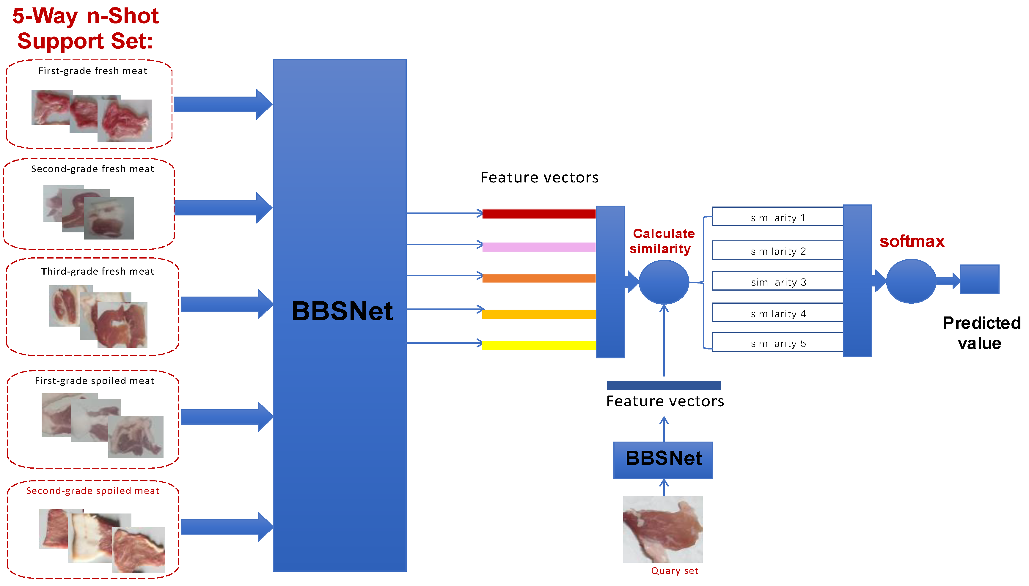
Figure 2.
Ilustration of BBSNet:(a) Basic structure of BBSNet;(b) Improved ShuffleNetv2,basic unit; (c) Improved ShuffleNetv2,spatial downsampling unit
Figure 2.
Ilustration of BBSNet:(a) Basic structure of BBSNet;(b) Improved ShuffleNetv2,basic unit; (c) Improved ShuffleNetv2,spatial downsampling unit
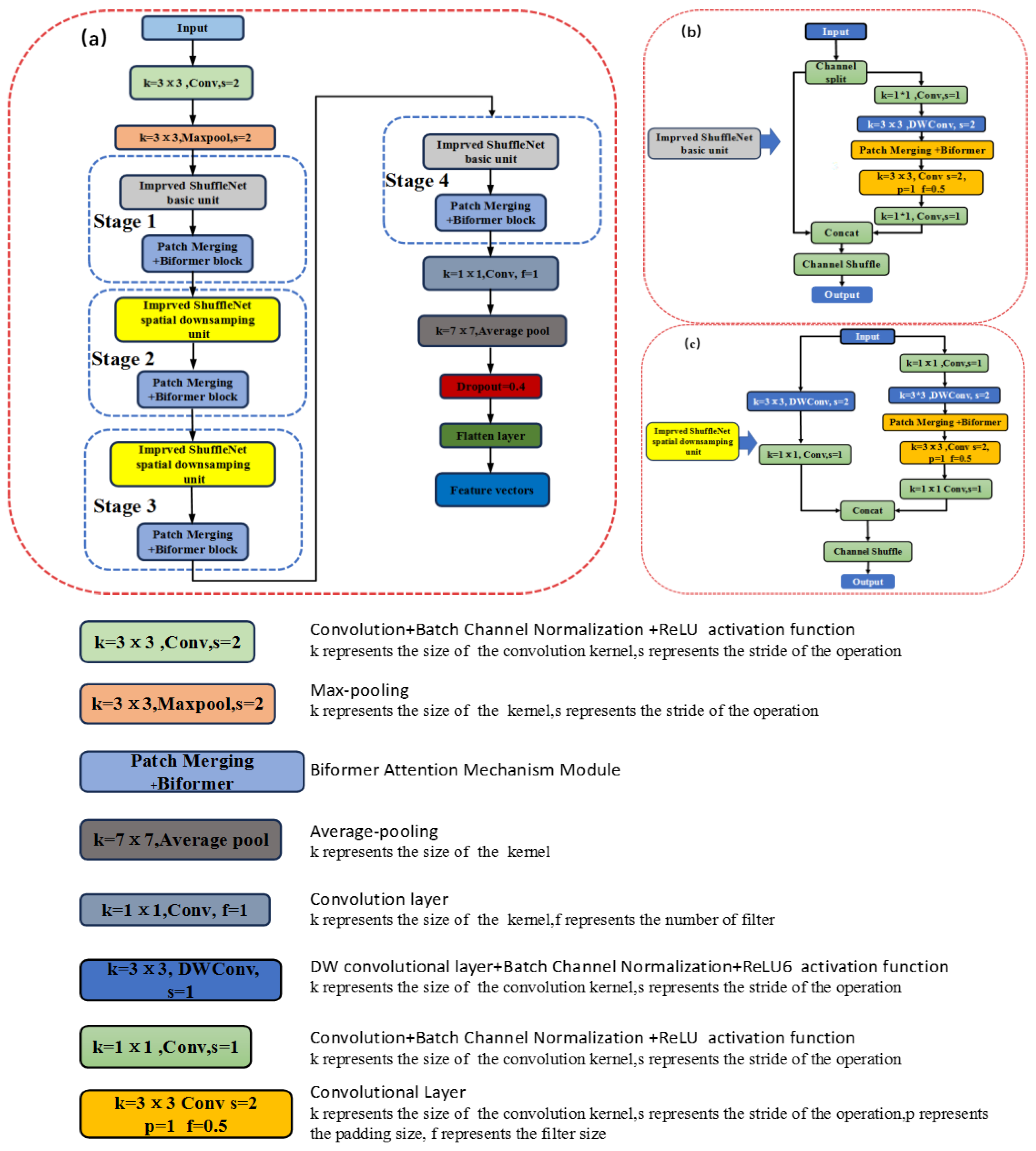
Figure 3.
Figure 3. Structure of improved Biformer
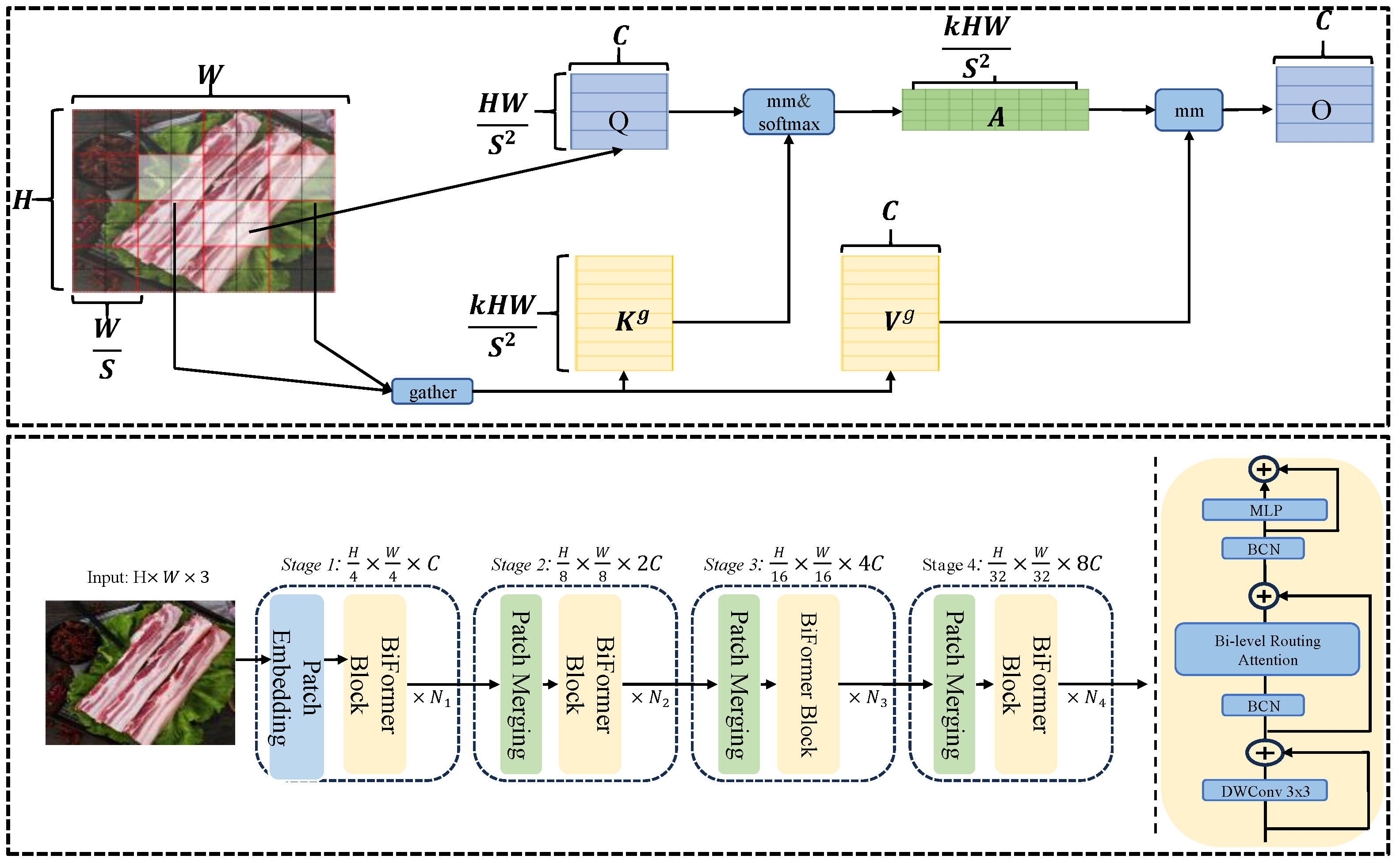
Figure 4.
Few-shot learning feature vector extraction and processing
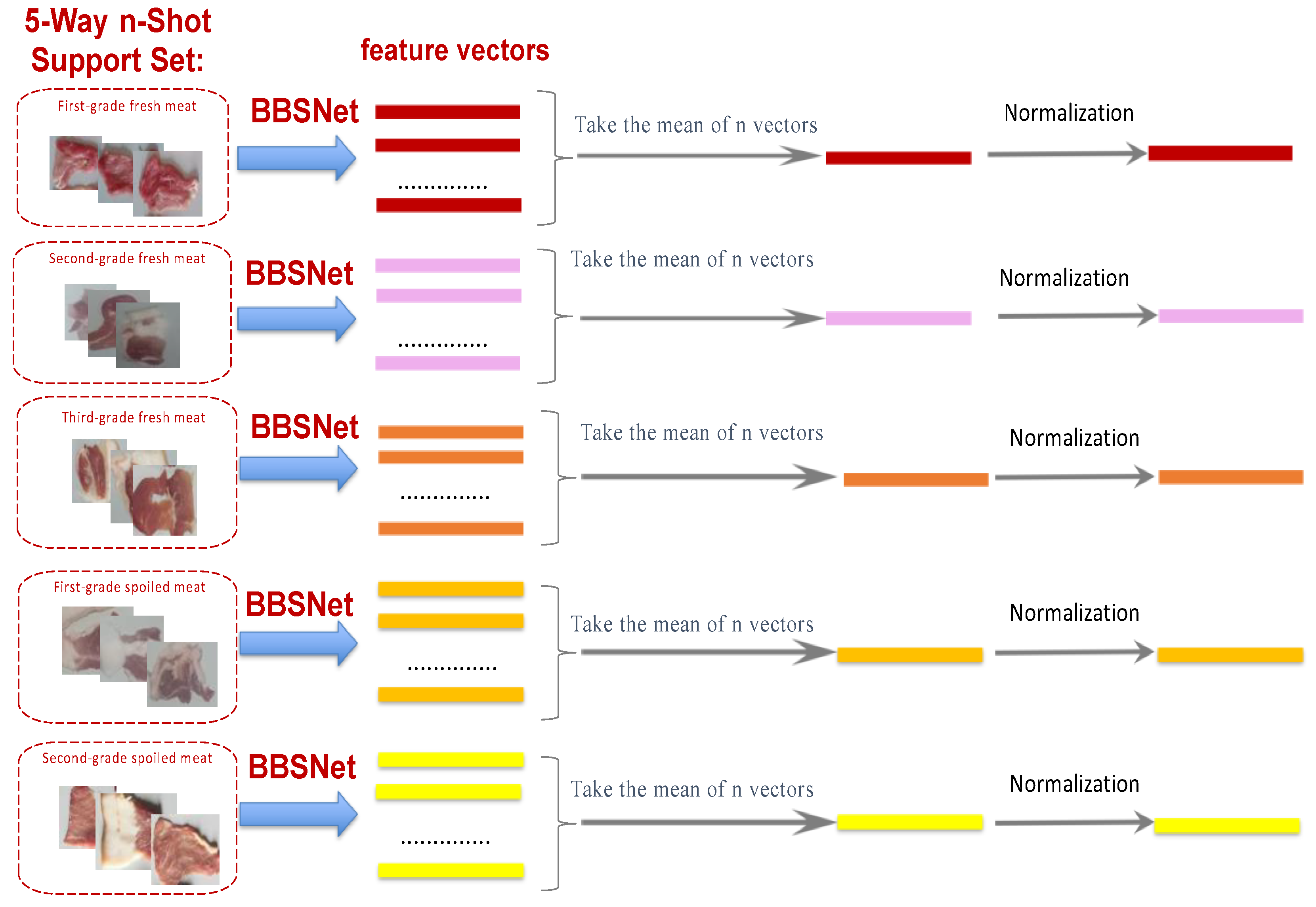
Figure 5.
Cosine similarity comparison.
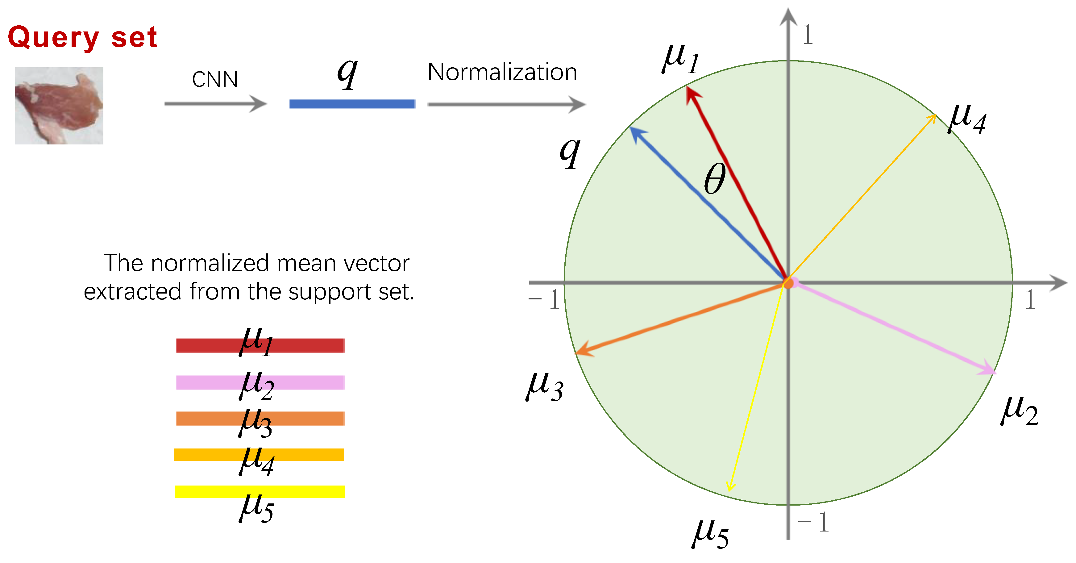
Figure 6.
The feature maps of pork freshness dataset.
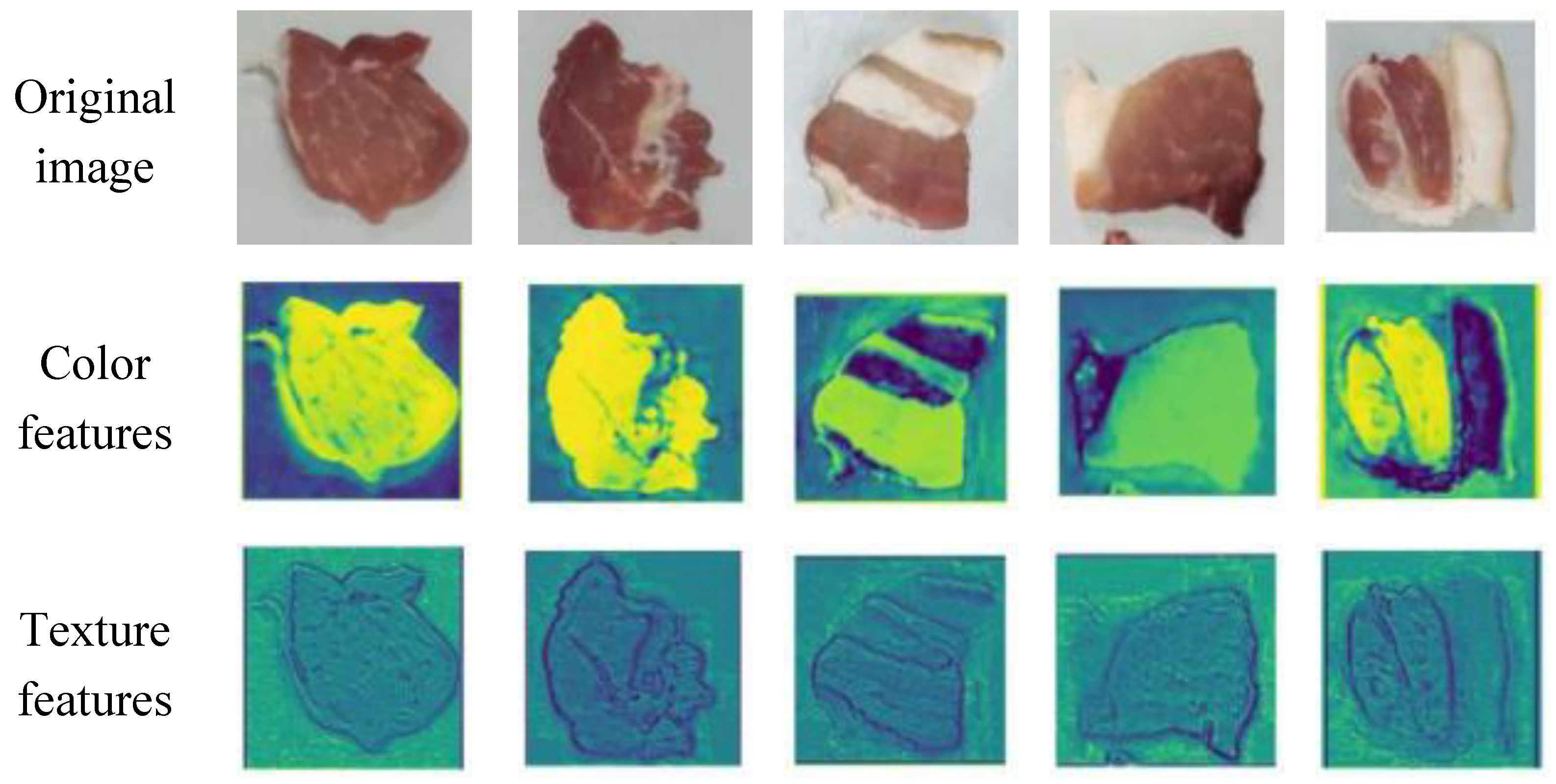
Figure 7.
The feature maps of Food101 dataset.
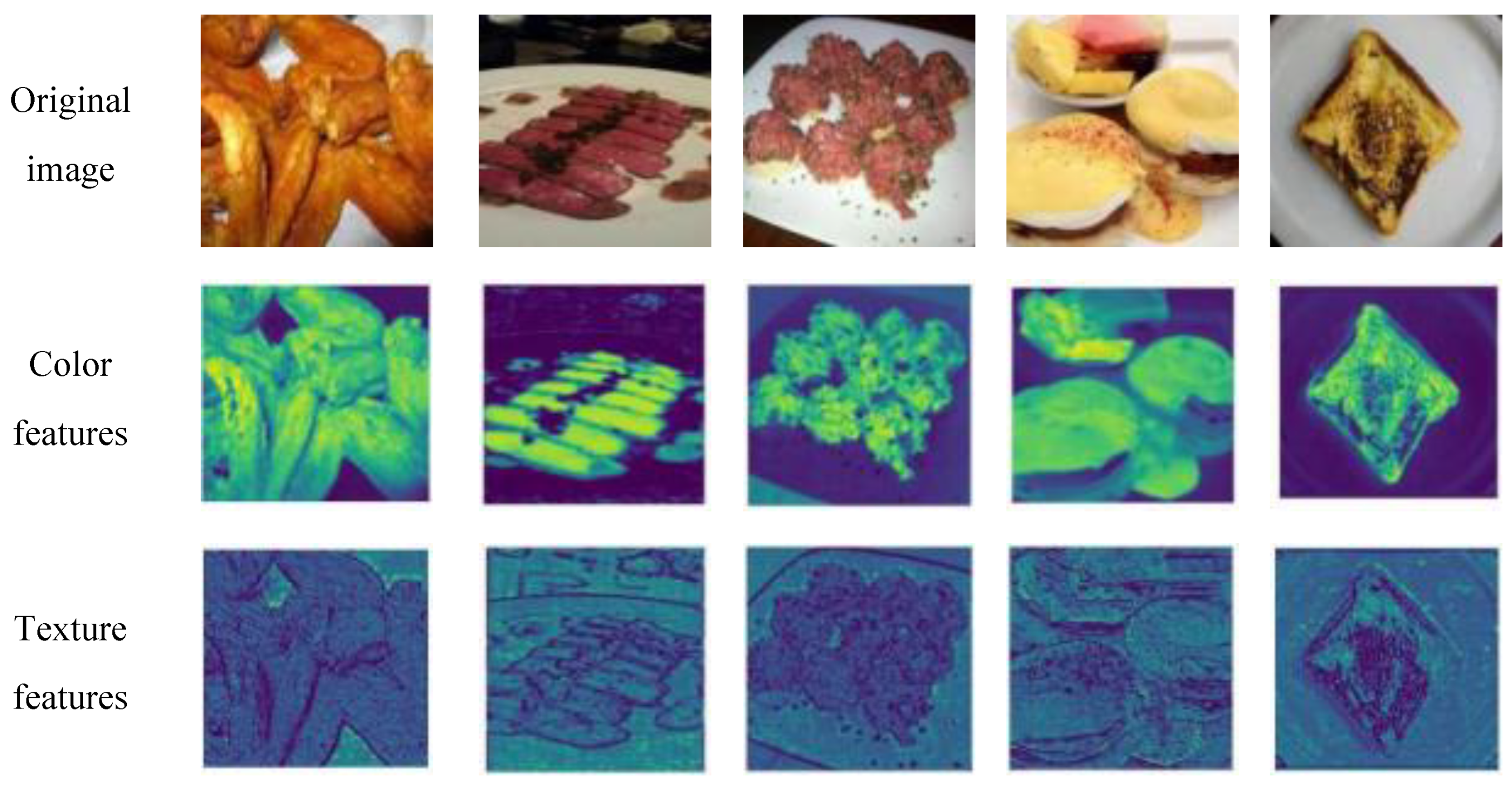

Table 1.
Main parameters of pork freshness grading.
| Freshness grade | Microbial Concentration (×103CFU/g) | Storage Time (h) |
|---|---|---|
| First-grade fresh pork | 4.168 | 0 |
| Second-grade fresh pork | 13.182 | 24 |
| Third-grade fresh pork | 301.995 | 48 |
| First-grade spoiled pork | 1778.279 | 72 |
| Second-grade spoiled pork | 5370.317 | 96 |
Table 2.
Pork freshness dataset analysis.
| Class | Image | Resolution |
|---|---|---|
| First-grade fresh meat |  |
224×224×3 |
| Second-grade fresh meat | 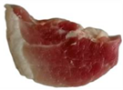 |
224×224×3 |
| Third-grade fresh meat | 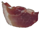 |
224×224×3 |
| First-grade spoiled meat | 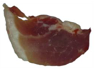 |
224×224×3 |
| Second-grade spoiled meat | 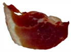 |
224×224×3 |
Table 3.
Mini-ImageNet Dataset overview.
| Training Set (83%) | Validation Set (12%) | Test Set (8%) | |
|---|---|---|---|
| Number of Categories | 80 | 12 | 8 |
| Number of Samples | 49800 | 7200 | 4800 |
Table 4.
Performance comparison of classical few-shot models.
| Model | Backbone | Comparison function | 5way,1-shot Accuracy (%) | 5way, 5-shot Accuracy (%) |
|---|---|---|---|---|
| Matching Net | ResNet-18 | Cosine similarity. | 48.12 | 67.20 |
| Prototypical networks | ResNet-18 | Euclidean distance. | 44.56 | 54.31 |
| Relation Net | ResNet-18 | — | 51.44 | 63.12 |
| Ours | ShuffleNetV2 + Biformer | Cosine similarity. | 59.72 | 78.84 |
Table 5.
Ours method vs. other methods on meat freshness dataset.
| Method Results |
Input image size | Batch size | Number of parameters (M) | Accuracy (%) | Sensitivity(%) | Specificity(%) | Precision(%) |
|---|---|---|---|---|---|---|---|
| AlexNet | 224*224*3 | 2 | 60 | 52.13 | 57.96 | 44.64 | 77.57 |
| VGG16 | 224*224*3 | 2 | 138 | 52.42 | 69.74 | 75.30 | 70.31 |
| GoogLeNet | 224*224*3 | 2 | 7 | 58.24 | 69.61 | 52.56 | 70.43 |
| ResNet50 | 224*224*3 | 2 | 25.6 | 68.43 | 79.33 | 74.78 | 69.29 |
| Ours | 224*224*3 | 2 | 2.3 | 96.36 | 78.85 | 85.71 | 96.35 |
Table 6.
The impacts of different normalization methods on model performance.
| Model | 5way 1-shot Accuracy (%) | 5way 5-shot Accuracy (%) |
|---|---|---|
| ShuffleNetV2+BN,BiFormer+LN | 48.23 | 63.25 |
| ShuffleNetV2+BCN,BiFormer+LN | 49.56 | 64.18 |
| ShuffleNetV2+BN,BiFormer+BCN | 51.49 | 68.31 |
| ShuffleNetV2+BCN,BiFormer+BCN | 52.44 | 69.52 |
Table 7.
The impact of improved BiFormer on model performance.
| Model | 5way, 1-shot Accuracy (%) | 5way, 5-shot Accuracy (%) |
|---|---|---|
| ShuffleNetV2, Backbone | 52.44 | 69.52 |
| ShuffleNetV2+BCN-BiFormer,Backbone | 55.73 | 69.62 |
| ShuffleNetV2, Backbone+BCN-BiFormer | 57.91 | 71.61 |
| ShuffleNetV2+BCN-BiFormer, Backbone+BCN-BiFormer | 59.72 | 78.84 |
Table 8.
Accuracy of Models with Different Support Set Sample Numbers.
| Fine-tuning | 1-Shot Accuracy (%) |
5-Shot Accuracy (%) |
10-Shot Accuracy (%) |
20-Shot Accuracy (%) |
40-Shot Accuracy (%) |
80-Shot Accuracy (%) |
100-Shot Accuracy (%) |
120-Shot Accuracy (%) |
|---|---|---|---|---|---|---|---|---|
| × | 56.64 | 71.55 | 76.29 | 83.46 | 85.81 | 87.21 | 87.19 | 87.20 |
| √ | 59.72 | 78.84 | 83.44 | 91.25 | 94.44 | 96.36 | 96.32 | 96.33 |
Table 9.
Performance Metrics of Few-Shot Learning Model with Varying Query Set Sizes.
| Query set sample size | Accuracy (%) | Training time (min) |
|---|---|---|
| 5 | 56.64 | 12.3 |
| 10 | 68.55 | 15.1 |
| 15 | 71.29 | 18.9 |
| 20 | 73.46 | 22.5 |
| 25 | 78.84 | 26.8 |
| 30 | 77.21 | 31.4 |
| 35 | 77.19 | 35.6 |
Table 10.
Comparative performance metrics of BBSNet across Food101 and pork freshness datasets.
| Dataset Name. | Accuracy (%) | Sensitivity (%) | Specificity (%) | Precision (%) |
|---|---|---|---|---|
| Food101 | 92.4 | 89.6 | 94.1 | 91.8 |
| Pork freshness | 96.36 | 78.85 | 85.71 | 96.35 |
Disclaimer/Publisher’s Note: The statements, opinions and data contained in all publications are solely those of the individual author(s) and contributor(s) and not of MDPI and/or the editor(s). MDPI and/or the editor(s) disclaim responsibility for any injury to people or property resulting from any ideas, methods, instructions or products referred to in the content. |
© 2025 by the authors. Licensee MDPI, Basel, Switzerland. This article is an open access article distributed under the terms and conditions of the Creative Commons Attribution (CC BY) license (http://creativecommons.org/licenses/by/4.0/).
Copyright: This open access article is published under a Creative Commons CC BY 4.0 license, which permit the free download, distribution, and reuse, provided that the author and preprint are cited in any reuse.


